A Mathematical Framework for the Japanese Agricultural Model

Onishi, H.H.

IIASA Working Paper

WP-80-156

October 1980

Onishi HH (1980). A Mathematical Framework for the Japanese Agricultural Model. IIASA Working Paper. IIASA, Laxenburg, Austria: WP­80­156 Copyright © 1980 by the author(s). http://pure.iiasa.ac.at/id/eprint/1313/ 

Working Papers on work of the International Institute for Applied Systems Analysis receive only limited review. Views or 

opinions expressed herein do not necessarily represent those of the Institute, its National Member Organizations, or other organizations supporting the work. All rights reserved. Permission to make digital or hard copies of all or part of this work 

for personal or classroom use is granted without fee provided that copies are not made or distributed for profit or commercial advantage. All copies must bear this notice and the full citation on the first page. For other purposes, to republish, to post on servers or to redistribute to lists, permission must be sought by contacting repository@iiasa.ac.at 

NOT FOR QUOTATIOR WITHOUT PERMISSIOS OF THE AUTHOR

A MATKEMATICAL FRAMEWORK FOR THE JAPANESE AGRICULTURAL MODEL

October 1980 WP-BO- 156

Working Papers are interim reports on work of the 1nternati~;lal Institute for. Applied Systems Analysis and have received only limited review. Views or opinions expressed herein do not necessarily represent those of the Institute or of its National Member Organizations.

INTE~KNATIONAL INSTITUTE FOR APPLIED SYSTEMS ANLALYSI S A-2361 Laxenburg, Austria

FOREWORD

Understanding the nature and dimension of the food problem and the poli- cies available t o alleviatp it has been the focal point of the lIASA Food and Agri- culture Program since it began in 1977.

National food systems are highly interdependent, and yet the major policy options exist a t the national level. Therefore, t o explore these options, i t is nect:ssary both to develop policy models for national economies and to link t.heni hogether by trade and capital transfers. For grea ter realism, the models in this scheme of anlysis a re being kept descriptive, ra ther than normntive. In the end i t is proposed t o link models of twenty countries, which together account For nearly 80 per cent OF important agricultural attributes such as area, production, population, exports, imports and so on.

In this paper Dr. Onishi describes a mathematical framework for an agricul- tural policy model for Japan.

Kirit S. Parikh Acting Leader Food and Agriculture P rogran~

PREFACE

The Food and Agriculture Program of IIASA started in 1977. Since that time, methodology, simplified national models, and some detailed national models have progressed. In 1980. Japan joined the Program.

Japanese agriculture is protected by various kinds of policies such as pro- ducer price support policies, import tariff and quota policies and taxation poli- cies. As a result, the production costs of many agricultural commodities in Japan are much higher than those of other countries. I t is quite interesting to see what would happen to Japanese agriculture if the producer price of rice were set at the international rice price. If the import quota of beef and pork are entirely removed, could steer and hog production in Japan still continue? If Japan exports rice, would U.S. farmers' incomes be reduced? What kind of poli- cies are effective for the alleviation of the world hunger problem? If we can experiment on even some of these problems through a world food model, Japan's participation in the Food and Agriculture Program could have some significance.

I would like to express my deep appreciation to Director R. Levien and Pro- gram Leader F. Rabar. Finally, I am grateful to Ms. Cynthia Enzlberger and Ms. Bonriie Riley for their patient typing and retyping of this paper.

Haruo ONISHI July 1980

CONTENTS

THE PURPOSE OF THE FOOD AND AGRICULTURE PROGRM

LINKAGE REQUIREMENTS FOR A WORLD MODEL

THE OBJECTS OF MODELING JAPANESE AGRICULTURE

COMMODITY LIST

STRUCTURE OF THE MODEL

EXPLANATIONS OF THE JAPANESE AGRICULTURAL MODEL Market Clearance and Social Account Module Demand for Commodi t ies Domestic Suppl ies of Commodi t ies Excess D e m a n d s for Commodi t ies Agricul tural , F a r m and R u r a l Incomes U r b a n Income Nonagricul tural r e v e n u e Government R e v e n u e and Expendi ture Cross Nat ional Product, Nat ional Income, a n d Ceneral R i c e Level Population, Labor Availability, Household, and Land Availability Module R u r a l and U r b a n Populat ion Labor Avai labi l i ty Household Przddy and Upland Field Avai labi l i ty Consumption and Intermediate Demand Module H u m a n Consump t ion Government C o n s u m p t i o n Irxtermediate Demand Animal Consumpt ion N u t r i t i o n Agricultural Production Module Product ion of Wheat Product ion of Bovine Meat and Milk Nonagricultural Production and Government Employment Module Nonagricul tural Labor E m p l o y m e n t , Wage Rate , Cupital Use Rate , and Product ion Government E m p l o y m e n t Investment and Capital Formation Module

Investment Capital Formation Depreciation of Capital International Trade, Price Deterrnination, Net Import Quota, and Buffer Stock Constraint Module International Trade und Price Determination Net Import Quota Buf ler Stock Constraint Government Policy Module Price Support PO licies Agricultural Productiun Policies International Trade Policies Tazat ion Policies

CONCLUDING REMARKS

AF'PENDIX 1 A Mathematicid Framework for t he Japanese Agricl~ltural Model

APPENDIX 2 Variable Notation

REFERENCES

. .. - V l l l

1. T H E P U R P O S E O F T H E FOOD A N D AGRICULTURE PROGRAM The oil crisis in 1973 and the food crisis in 1974 affected the world economy

seriously. These crises have lead to many people paying more attention to glo- bal rather than national problems and to recognizing tha t economic gro-vth is not unlimited. A few years later, the Food and Agriculture Program a t IIA54 was established to: - evaluate the nature and dimensions of the world food situation, - identify the factors affecting it, and - find alternative policy action a t the national, regional and global level.

Using the da ta and evaluations from this study it is hoped tha t solutions to alleviate existing and emerging food problems in the world can be found.*

*"Local Problems in a Global System (The Approach of IIASA's Food and Agriculture P r e gram)", F. Rabar, FAP Newsletter No. 3, August 1979, p. 5 .

2. LINKAGE REQUIREMENTS FOR A WORLD MODEL A general equilibrium approach is taken to a world agricultural model. A

variety of national agricultural models which reflect the characteristics of each country's agriculture are linked to a world agricultural model. To integrate many national models into a world agricultural model several conditions are imposed on each national agricultural model.

They are required (a) for a common goal of all countries and (b) for guaran- teeing the existence of an equilibrium in a world agricultural model. They are the following: *

1) The IIASA commodity list should be accepted. I t is possible to introduce more commodities than there are on the commodity list, but they must be only those productas which participate in international exchange and which are defined by the list.

2) The time horizon will be 15 years and the time increment one year.

3) There is a one-year time lag after the production decisions are made. Pro- duction is given a t the time point of exchange.

4) The rnodels should be closed: The rest of the economy should be represented in one aggregated commodity.

5) Government policies should be explicitly formulated.

6) The models should behave as continuous, nonsmooth excess demand func- tions of international prices.

7) Excess demand functions are homogeneous of degree zero in international prices and incomes.?

3. THE OBJECTS OF MODELING JAPANESE AGRICULTURE

Japanese agriculture is closely related to agriculture and nonagriculture in the rest of the world. It is impossible to predict the effects of government poli- cies on Japanese agriculture from an analysis of an agricultural sector model or even a Japanese economy model, because there are some reactions to govern- ment policies for Japanese agriculture from the rest of the world. Hence, it is of great importance to evaluate quantitative1.y the "net" effects of agricultural poli- cies, trade policies, and taxation policies set by the Japanese government on Japanese agriculture in a global framework.

The purpose of this research is:

(1) to evaluate quantitatively the effects of agricultural policies, trade policies, and taxation policies regarding Japanese agriculture,

(2) to pursue appropriate labor allocation, land use, and capital formation, and

(3) to predict incomes and food consumption patterns in rural and urban areas between 1981 and 1995.

4. COMMODITY LIST The commodities to be introduced into the production module differ from

those listed in the Food and Agriculture Program a t IIASA. In order to reflect the characteristics of Japanese agriculture in the model, 28 agricultural com- modities are selected. All products and services in the rest of the national

*FAP Newsletter No. 3, August, 1979, pp. 30-31. tKeyzer. M.A.. A n Outline of IIASKs Food and Agriculture Model. January, 1980, p. 8.

produc:tion are t reated as one aggregate nonagricultural commodity. However, i t is possible to disaggregate the nonagricultural commodity into three commo- dities (a) capital goods, (b) consumption goods and services, and (c) minerals and energy, in a future version of the Japanese Agricultural Model, JAM. The commodity lists of IIASA and JAM are:

11 ASA JAM

Wheat 1. Rice 2. Coarse grain 3. Oi l and fats 4. Protein feeds 5. Sugar 6. Bovine meats 7. Pork 8. Poultry and eggs 9. Dairy products 10. Vegatables 11. Fruit and nuts 12. Fish 13. Coffee 14. Cocoa and tea 15. Alcoholic beverages 16. Clothing fibers 17. Industrial crops 18. Noriagricultural commodities 19.

( the res t of the national production)

20. 2 1. 22. 23. 24. 25. 26. 27. 28. 29.

Wheat Rice Barley Rye and oats Corn Oil and fats Protein feed Sugar beets Sugar cane Nonprotein feed Bovine mea t Pork Poultry Egg s Dairy products Starchy roots Soybeans Vegetables Grapes

Other fruit Fish Tea Alcoholic beverages Tobiicco Silk cocoons Ingusa plants Green feed Wood Nonagricultural commodities

(the res t of the national production)

5. STRUCTURE OF THE MODEL The model represents the Japanese economy and puts emphasis oil the

agricultural sector. The s t ruc ture of the JAM consists of the following eight modules:

(1) Market clearance and social account,

(2) Population, labor availability, household and land availability, (3) Consumption and intermediate demand.

(4) Agricultural production,

(5) Nonagricultural production and government employment,

(6) Investment and capital formation.

(7) International trade, price determination, net import quota, and buffer stock constraint, and

(8) Government policy.

The market clearance and social account module represents commodity balances, incomes, corporate profit, government revenues and expenditures, and gross national product.

The population, labor availability, household and land availability module is related to rural and urban population, rural and urban labor availabilities, numbers of rural and urban households, and acreages of paddy and upland fields.

The consumption and intermediate demand module deals with human. government, and animal consumption of agricultural and nonagricultural com- modities, and intermediate demand for agricultural commodities which are used for the production of alcoholic beverages (sake, beer. whiskey, and wine), oil (vegetable oil and fish oil) and protein feed (soybean cake and fish cake).

The agricultural production module shows acreages of crops, labor alloca- tion, capital allocation, nitrogen fertilizer application, production of crops, animals, fish and wood, expected producer price formation, and producer prices of disaggregated commodities.

The nonagricultural production and government employment module states workir\g hours per worker during a year, capital use rate, wage rate of nonagri- cultural production, employment and production.

The investment and capital formation module deals with investments by gover-nment, farmers (including fishermen and forestry workers) and enter- prises, savings, capital formation and depreciation of capital.

In the international. trade, price determinati.on, net import quota and buffer stock constraint module, net imports, upper and lower bounds of net imports quota, buffer stocks, upper and lower bounds of buffer stocks, relations between IIASA's world prices and world prices with which Japan is faced (in terms of 1970 base year.), consumer prices, and producer prices are discussed.

Finally, tax rates, producer and consumer prices for wheat, rice and tobacco, tariff rates, subsidies, government wage rate, and imports of government-controlled commodities are det.ermined in the government policy module.

6. EXPLANATIONS OF THE JAPANESE AGRICULTURAI. MODEL (JAM) Let 11s give brief explanations of most. of the equations and identities in the

model. The whole set of simultaneous equations rnodel JAM and Variable Nota-

FLOW CHART OF JAM

Invest GN

A: Agricultural Sector N: Nonagricultural Sector G: Government U : determined

- Invest GA I

1 ALLOCATION 1

t Producer

Capital GA ] Price t

Tax A

Fe r t i l i ze r I' Consumer

Net Consump. A - Price 11 Import 1

Invest A Buffer

Demand '* 1

Stock v1 I

I n t . Rate

Invest N *Capital N

1 Labr Producer Price

O : given

J =.

Invest A

Land

,*Capital A

Labor A

A

1 World Price

r Ag. Prod.

tion is given in the Appendix.

6.1. Market Clearance and Social Account Module

6.1.1. Demand for Commodities

As far as wheat and rice are concerned, the commodities supplied from farmers and traded in the international market are not the same as those con- sumed. I-Iulled wheat and rice are supplied and traded, while wheat flour and polished rice a r e consumed. It is assumed that the commodities wheat, rice, coarse grains, bovine meat, pork and nonagricultural commodities can be stored. while all other commodities are perishable. The commodities rice, coarse grains, vegetables, fruit and fish can be used for processed commodities. Nonagricultural commodities are used as consumption goods, investment goods and intermediate goods.

6.1.2. Domestic Supplies of Commodities

Commodities produced a re consumed one year later in order to satisfy the common requirements of IIASA's general equilibrium system.

6.1.3. Excess Demands for Commodities

Excess demand is defined a s total consumption minus total domestic sup- ply. 1f excess demand is positive, i t is regarded as import. On the other hand, if excess demand is negative, it is regarded as export. The reduced forms of excess demand function must be homogeneous of degree zero in IIASA's world prices.

6.1.4. Agricultural. Fa rm a n d Rural Incomes

Crop income of crop i, CIi, is defined as the gross sales of crop i minus the cost for intermediate goods used for production of crop i. Animal income of animal i. AIi, is accounted as the gross sales of animal i (including the joint pro- ducts) minus the cost for intermediate goocis and feeds. The allowances for cap- ital depreciation are determined by a function of total capital in agriculture. Agricultural income AGIN is defined as the sum of farming income FART, fishery income FISI, and forestry income FORI, where farming income implies the sum of all crop and animal incomes. Farm income FI consists of agricultural income AGIN, r~onagricultural income NMI, net income transfer from overseas ITOF. dividend DIVF, and subsidies from fallow paddy fields ARP2-ARZ. Rural income RI includes the income t,ransfer (subsidies) from the government. Per capita incomes and per household incomes are defined for convenience.

6.1 -5. Urban 11lcome

Urban income U I consists of wage incomes UWI from nonagricultural pro- duction and government work, dividend DIVU, and net income transfer from overseas ITOU. Disposable urban income IIUI is obtained from the subtraction of nonagricultural persorlal tax NPTX-UI frorri urban income. Per capita urban income and per household urban income a re introduced for convenience.

6.1.6. Nonagricultural revenue

The previous year's production brings the curren-t gross revenue NC19-NQ1.9-1 due to the common requirements for the IlASA linkage system. Gross profit is defined as the gross revenue plus ne t income transfer from over- seas ITON minus indirect tax II'XN-NC19.NQ19-1 :minus wage WRNmENAL minus

allowances for capital depreciation DAN. Capital depreciation allowances are considered to be a function of capital stock KN and capital use ra te KURN. Divi- dend DIVI is determined by gross profit GP19. Then. retained earnings RE is defined as the gross profit plus capital depreciation allowances minus corporate tax CTX-GP19 and dividend DIVI. Dividend is divided into dividend to farmers (including fishermen and forest workers) and dividend to urban dwellers.

6.1.7. Government Revenue a n d Expenditure

The government including central and local collects personal taxes FI-M3TX and UI-NPTX. indirect taxes CP6.DG-ITXS, CPlG.Dl6-ITXB, and CPlS.Q19.ITXN, cor- porate tax GP19.CTX. tariffs zT~i -Mi .wPi sales of wheat, rice and t;obacco CP1-Dl, CP2G-D2G, and C18T-QlBT, and net income transfer from overseas ITOG.

On the other hand, the government spends money on the consumption and investment of nonagricultural commodities CP19-(IG+CG), purchases of wheat, rice, and tobacco from farmers and overseas, PPl.Ql, WP1.Ml. PP2G.Q2G, P18TeQ18T. and WlEiT*MlEiT, income transfer t o agriculture SUBA, subsidies for fallow paddy fields ARP2.AR2, and wages for government employees WRG-LGOV.

6.1.8. Gross National Product, National Income. and General Price Level.

Gross national product GNP is defined as the sum of the gross incomes zPPi.Qi_l of all commodities divided by general price level GPL. The general price level is obtained as the Laspires index. National income NAIN is the sum of agricult,ural income AGIN and nonagricultural income NPIS.NQl9.

6.2. Population, Labw Availability, Household, a n d Land Availability Module.

6.2.1. Rura l and Urban Population

Change in population is influenced by various factors such as demographic, econornic, arld social factors. It is quite difficult to explain the change in popula- tion only by economic factors. Hence, total population in Japan is treated. a s exogenous in the model. Given total population, rural and-urban popul.ation are derived. Rural population is a function of total population TPOP, rural and urban standard of 1.iving represented by per. capita disposable rural-urban income ratio (PDRI/'PDUI)_l, government investment IGA-, in agriculture and rural activities to make rural life attra.ctive, and pressure of urban ~verpopulation reflecting high living costs, high land price, high food pric:e. I.ac:k of sewage system, etc. (UPOP/TPOP)_l. Then, urban population is de:fined as the subtraction of rural popula.tion from total population.

6.2.2. Labor Availability

Total labor availability LAR in rural areas is determined by rural popul a t ' .ion RPOP, rdtio of rural household expenditures on food, beverages and housing over rural tlisposable household income (REF'H/DRHI)-l representing rural st.andard of living, and time trend variable indirectly representing the situation in which people in rural areas t ry t o ge t higher edut-alion and as a result the age a t which they d a r t work is later.

Labor avai1abilit.y in rural areas is used up by labor for farming (crop and animal production), LFAR, labor for fishery LF'IS, labor for fo reshy work LFOR and nonagricultural productiori LNAR (including part-time jobs). Labor availabil- ity in urban areas LAU is determined by urban population, ratio of urban house- hold expenditures or1 food, beverages and housing over disposable urban house- hold income, and time trend variable. The rnearlirigs of these explanalory vari- ables are similar to those of labor availability irl rurSal areas.

6.2.3. Household

The numbers of rural and urban households are determined in the model by the respective popu la t io~~ and time trend variable.

6.2.4. Paddy a n d Upland Field Availability

Paddy field acreage availability is the previous year's paddy field acreage minus the sum of additional land acreage used for urbanization and further industrialization and the acreage of paddy field changed into upland field. The definition of upland field acreage can be easily understood through the definition of paddy field acreage. The acreage of additional land used for urbanization and further industrialization is affected by changes in GNP AGNP-1, retained earnings RE-l, change in urban population AUPOP, and time trend variable t. The ratio of paddy and upland field deteriorated by urbanization and further industrializa- tion is fixed in the model.

The change of paddy field into upland field depends on rice production reduction policy variable ARPZhI and r-atio of land productivit.ies of rice and dairy products in terms of incomes (C12/A2)_1/(A110/AGF)_I.

6.3. Consumption and Intermediate Demand Module

6.3.1. Human Consumplion

Linear expenditure system is adopted for rural and urban human consump- tion. Total rural and urban household expenditure RHE and UHE are functions of respective disposable household incomes DRISI and DUHI and ratios of respec- tive population over labor engaged in agricultural and nonagricultural produc- tion RPOP/LAR and UPOP/EUL. Rural and urban expenditure on the i-th consurner's com~nodity REi and UEi are determined by the respective linear expenditure systems, where rural and urban committetl consumptions of the i- th consumer's commodity are expressed by RCi and UCi respectively.

6.3.2. Government Consump tion

It is assumed that the government does not, consume agricultural commodi- ties but consumes nonagricultural commodities. The government consumption of nonagricultural commodities is determined by real government revenue CR/ CP19 and real national income (NAIN/CPIS)-~. The last explanatory variable represents a little Keynesian influence.

6.3.3. Intermediate Demand

Rice, coarse grains, starchy roots, soybeans, vegetatlles (sesame seeds, rape seeds, etc.), grape arid fish are used for the production of processed com- modities such as alcoholic beverages (sake or rice wine, beer, whiskey. wine), oil and cakes. Nonagricultural commodities used as intermediate goods a r e nitro- gen fertilizer, viriyl sheet, ne t , chemicals, fuel oil, etc. Real national iricome, the previous year's intermediate demand quantity, consumer pric e ratio, and time trend variable a re corlsidered to determine intermediate demands.

6.3.4. Animal Consuznption

Protein feed, non-protein feed, and green feed are consumed by steers. bulls, cows, pigs, broilers and hens. It is assumed that the consumption quanti- ties of protein, non-prolein, and green feed per head of animal are fixed and half of the animals slaughtered (or consumed) had consumed these feeds.

6.3.5. Nutrition

Per capita protein, carbohydrates, and fats are calculated for rural and urban dwellers.

6.4. Agricultural Production Module

Twenty-eight agricultural commodities are focussed on. Instead of men- tioning all of the 28 submodules of agricultural production module, we would like to concentrate only on wheat production and bovine and milk production, because it is not difficult to understand other submodules.

First of all, it is assumed that the production decision time differs from the harvest and exchange time and the farmers would like to maximize the expected farming income subject to acreage, nitrogen fertilizer, capital and labor con- straints.

We can set up a basic problem as follows:

max z ( P ~ i * - ai).Qi Ai,Li.Ki.Ni.NFi

subject t.o

A2 5 APF

Ki 5 KFAR 3 z NFi I; NFTL

i= 1

where

for wheat, rice, and coarse grains

for other crops.

for an.imals, and

with the Box-Jenkins approach

where

ai-Qi cienot.es the cost of intermediate goods and/or feeds and all variable nota- tions car) be found i.n the appendix Variable Notations.

The average working days per farmer during a year W H R is determined by capital-labor ratio (KF'AR + KFIS + KFOR)/ (LFAR + LFlS + LFOR) and the previ- ous year's real per capita rural income (PDRI/CP2)-I. The total quantity NFTL of nitrogen fertilizer is determined first and then it is used for various crops. I t is a func:tion of the previous year's quantity NFTL1, the previous year's real czrop income, and the previous year's real nitrogen fertilizer price (PNF/PP2)-I. The nitrogen fertilizer price PNF depends on the nitrogen fertilizer quantity NFTL. the previous year's nitrogen fertilizer price PNF_I. and consumer price of nonagricultural commodities CP 19.

6.4.1. Production of Wheat

In the production of wheat, it is assumed. t.hat farmers anticipate the expected wheat producer. price P P l * through the Box-Jenkins formulation. The acreage of wheat A 1 is determined by the previous year's acreage Al.l and the ratio of expected wheat income per farmer over wage ra t e of nonagricultural production (PP1*-Q1~l)/(WRN-l.L1.l). The nitrogen fertilizer quantity applied per acre of wheat NFl/Al is determined by the previous year's application quantity (NF1/Al).l and the expected wheat producer price divided by nitrogen fertilizer price PPl*/PNF. Since A1 is predetermined for this equation, the nitrogen fer- tilizer quantity used for wheat production can be derived a s NF1. The capital used for wheat production K 1 is a function of the previous year 's capital use K1_l and capital labor rat io KFAR/LFAR. The amount of labor used for wheat produc- tion L1 in t e rms of man d.ays is determi-ned by the previous year's labor L1-l and the ratio of expected wheat income per farmer over wage ra te of nonagricultural production (PP I*-Q l ~ ) / (WRN.l.L1.l). Accordingly, t h e production function of wheat is specified as a function of acreage, nitrogen fertilizer application quan- tity, private capit.al used, government capital, labor, weather index, and time t rend variable. Instead of production function, a wheat yield function can be considered. The final decision whether the production function is more suitable for wheat production in Japan than the yield function depends on estimation.

Since the submodules of other crops are similar to the submodule of wheat production, we would like to skip them and refer t o tohe production of bovine meat and rnilk.

6.4.2. Production of Bovine Meat and Milk

The number of s teers N7 is determined by the net birth r a t e R7 and t.he number of s teers surviving at. the end of the previous year NS7.1. The ne t birth ra te is affected by the previous year's bovine m e a t price-pork price ratio (PP?/I'PB)-l, the previous year's bovike mea t price-mixed feed price ratio (PP?/PNF5)-l and time t rend variable t . Expected producer price of bovine meat PP7* is of Rox-Jenkins type. The number of slaughtered s t ee r s SL7 i c ; a function of the number of s teers N? and the ratio of expected bovine meat p r ~ c e over pork price PP7*/PP8-1. Then, the nunlber NS7 of s teers which (:an survive a t t he end of a year is determined as the nurrtber of s teers minus the number of slaughtered steers. The average weight of bovine mea t per head of s teer is a function of time trend variable. Government r e senrc l~ into animal husbandry may have helped to increase the average weight.

The number of cows is determined by the net birth ra te B10 and the number NF'lO-l of cows survlvirig a t the end of the previous year. Half the calves a re cows and the r e s t are raised as bulls for t h e production of bovine mezt . The ne t birth ra te is influenced by the milk price change PP10-l/PP10-2, average green feed intake QQGF/NF'lO.l, and t ime t r end variablet . The nurnber of cows slaughtered SF10 is deter-mined by the nurriber of cows N10, the previous year's ratio of bovine meat price over milk price ( P P ~ / P P ~ O ) - ~ , and t h e prodr~ction quantity of green feed QQGF. The number of cows which can survive a t the end of a year is obtained by subtaracting the number of cows slaughtered from t.he number of cows raised. The number of bulls slaughtered SMlO is determined by the number of bulls raised NM1O-l + 1/2-810-NF10 and the previous year 's ratio of bovine meat price over pork price (PP7/PP8)_1. The nunlber NMlO of bulls which can survive a t the end of a year is the number of raised bulls minus the number of slaught.ered bulls. Therefore, the prod uc:tion quantity of bovine mea t is the sum of the production quantities of bovine meat of st.eers, cows and bulls. On the other hand, the production quantity of milk is deterrnined by the number

of cows N10 - l/Z.SFlO and the average green feed intake QQGF/NF10 The capital K7 and labor L7 used for the production of bovine mea t are assumed to bc proportional to the number of s teers and bulls raised. Similarly, the capital K10 and labor 1, lO used for milk production are assumed to be proportional to the number of cows raised. The explanation of other submodules of animal, fish, and wood production is omitted, because it is easy to understand them.

6.5. Nonagricultural Production and Government Employment Module

6.5.1. Nanagricultural Labor Employment, Wage Rate. Capital Use Rate, and Production

The number of employees is determined not only by economic variables of real wage rate WRN/NP19 and capital-labor ratio KN/LNAP but also by the insti- tutional variable meaning the Japanese permanent employment system and represented by the previous year's employment level ENAL-I. Therefore, even if the real wage ra te increases substantially, employment may not go down much due tc the previous year 's employment level. The time lag number 1 of ENAL-1 implies that for a t least one year a considerable number of employees do not lose jobs as a result of a traditional employment custom even if a recession hits the Japanese economy.

There is an assumption that the labor from the rural a rea is always hired, so that this labor does not include the labor in rural areas which wished to find jobs in the nonagricultural sector but did not find them. However, the labor in rural areas which tried and failed to find jobs in nonagricultural production is always absorbed by agriculture. As a result, the labor engaged in agricultural production may include disguised unemployment. Unemployment is always in urban areas if i t occurs.

Average working days, in te rms of 8 hours per day, of a worker during a year WHN is a function of capital-labor ratio (KN+KGN)/LNAP including govern- ment capital in the nonagricultural sector, the previous year 's working days showing rigidity of working days WHN-l, per capita urban expenditure on food, beverages and housing (UEF'H-NUH)-l/UPOP-l which reflects the important aspects of the Japanese economy to be improved. and time trend variablet.

Capital use rate KURN is considered to be related to capital productivity change, inventory stock-production ratio, arld government investment change which is considered t o stimulate stagnant nonagricultural production.

Nonagricultural production is determined by a Cobb-Douglas production function of capital actually used KAUN, and total working days TWHN with con- s tant returns to scale. Hicks neutral technical progress is assumed to prevail in nonagricultural production. So far, nonagricultural product.ion quantity NQ19 has not included wood production quantity. IIASA's nonagricultural production quantity Q19 includes both non-IIASA nonagricultural production NQ19 quantity and wood production quantity QFOR.

6.5.2. Government Employment

Government employment is needed mainly for social services which are useful for daily life and private production. The national railroad, telephor~e and telegram, NHK (government broadcasting), etc. which a re semi-government enterprises are t rea ted as private enterprises in the model.

The number of government employees is determined by the total labor avai- lability for nonagricultural production LNAP and ratio WRG/WRN of government wage ra te and nonagricultural wage rate. The ratio of government employees

hired in rural areas over government employees hired in urban areas is treiibed as constant over time.

6.8. Investment and Capital Formation Module

6.6.1. Investment

I t is assumed tha t the government invests for an increase in social stability, national security, production efficiency, development and growth, whenever seri- ous social instability, deterioration of national security, stagnant economic activities, etc. occur. As explained in the government policy module, social sta- bility from an economic viewpoint'is related t o equity and opportunities for employment. National security is connected with national defense. protection of agricultural production, and storage of important commodities. Research and improvement of infrastructure make some contributions to efficiency, develop- ment, and growth. The main explanatory variables of government investment are the real national income (NAIN/GPL)-l and real government revenue (GR/ GPL)-l. However, since the government is bureaucratic, the previous year's real government investment IG-1 also influences the determination of current government investment IG. Government investment is divided into government investment in agriculture and rural activities denoted by IGA and government investment in the nonagricultural sector denoted by IGN. Government invest- ment in agriculture depends on the previous year's level IGAl, food self- sufficiency ra te FSSR-,, and the per capita agricultural-urban income ratio (PCAJ/PCUI)-I. Then, government investment in the nonagricultural sector IGN is defined as the remaining.

It is assumed that if the long-run desirable capital KN* exceeds the previous year's capital KN-l, there is an incentive t o invest in the nonagricultural sector. Thus, the long-run desirable investment IN* is

IN* = KN* - KN-1

Long-run desirable capital is considered to be a function of the long-run expected demand D*, the long-run expected domes-tic supply demand ratio DSDR*, the long-run expected capital use rate KURN*, and the long-run expected real profit ra te PR19*. Thus, we have

KN* = ~(D*.DsDR*,KURN*,PR~~*)

The product the of long-run expected demand and expected domestic supply-demand ratio is regarded as the long-run expected effective demand for nonagricultural commodities which the Japanese industry could satisfy. In other words, it is the long-run expected sales. The long-run expected sales a re assumed t o b e a function of arithmetically weighted average production quantity during the last three years, so that we have

D*.DSDR* = f(x(4-i).Q19-i/ 6)

The long-run expected capital use rate is assunled to be a function of arit,hrneti- cally weighted average capital use ra te during the last three years, so that w e have

3 KURN* = f ( z (4-i).KURN-J 6)

i= 1

The long-run expected real profit ra te is regarded as a function of arithmet- ically weighted average real profit rates during the last three years as shown by

Real retained earnings and real inkerest rates affect irlvestrnent in the nonagri- cult,ural sector. Accordingly, we have an investment function for the nonagricul- tural sector as follows:

Japanese agriculture heavily relies on government agricultural policies. The improvement of the infrastructure in rural areas, biological, economic and technical research, and extension work by the government improve agriculture. Farmers (including fishermen and forest owners) invest in agriculture if the long-run expected capital KA* exceeds the previous year's total capital in agri- culture (KFAR + KFIS + KFOR)-l. Thus we can write

IA* = KA* - (KFAR+KFIS+KFOR)-I

The long-run expected capital in agriculture depends on t h e long-run expected government capital in agriculture KGA* and the long-run expected real profit ra te PRA*, which a re expected not by the government but by farmers. However, since the long-run expected government capital KGA* is based on the long-run expected government investment in agriculture IGA*, we can write

The long-run expected government investment IGA* is considered to be a function of the arithmetically weighted average food self-sufficiency ra te during the last three years and arithmetically weighted average government invest- ment in agriculture during the last three years, so tha t we can write

IGA* = f(C(4-i).FSSR-i/ 6, C(4-i).IGki/ 6)

On the other hand. the government tax policy for agriculture and govern- ment subsidies (or income transfer) to agriculture influence the expectation for- mation of the long-run profit real rate. Therefore, we consider tha t the long-run real expected profit r a t e is a function of arithmetically weighted average real rural income during the last three years.

We can write

PRA* = f(( l /6)- ~(4-i) .RI. i /CP19-i . (KFAR + KFIS + KFOK)-i)

Accordingly, we consider tha t the private investment in agriculture, after real interest ra te is taken into consideration, ta.kes the following form:

IR, (KFAR + KFIS + KF0R)-1)

The investment in fishery lFIS out of total investrrlent in agriculture IA is determined by arithmetically weighted average production quantity of fishery during the last three years, the previous year 's investment in fishery, the ratio of fishery income over farming income per worker, and the previous year 's capi- tal in fishery. In a sim.ilar way, the investment in forestry IFOR is considered t o

be a function of arithmetically weighted average wood production quantity dur- ing the last three years, the previous year's investment in forestry, the ratio of forestry income over farming income per worker, and the previous year's capi- tal in forestry. Then, the remaining investment defined as IA-IFIS-IFOK goes to the farming subsector.

Savings KS, US, GS are defined as disposable incomes minus expenditures or government revenue minus government expenditure. Retained earnings RE are also taken into consideration. The investment in housing IH (rural and urban) is equal to total savings (RS + US + GS + RE)/CP19 minus subtotal invest- ments (IG + IA + IN).

6.6.2. Capital Formation

In general, the current capital stock is defined a s the previous year's capi- tal stock plus net investment. Net investment is equivalent to gross investment minus capital depreciation.

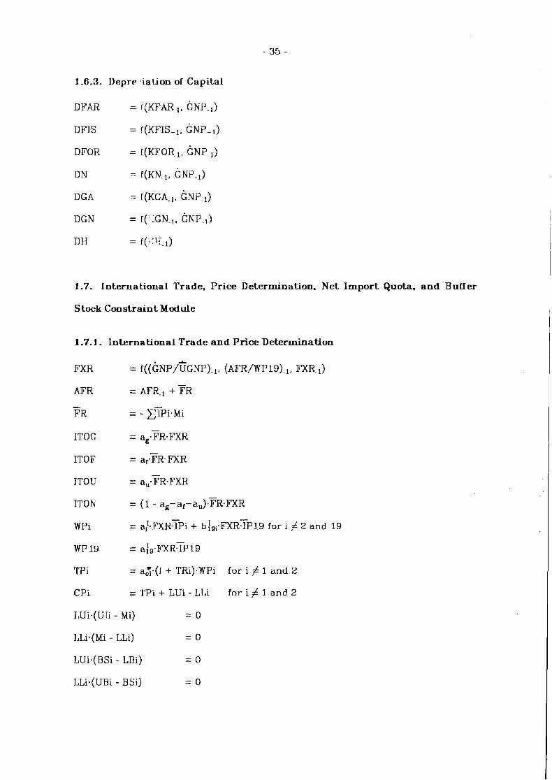
6.6.3. Depreciation of Capital

Depreciation of capital is mainly determined by the previous year's capital stock. However, if we think of rapid technical progress in Japan, capital rnay be replaced earlier than scheduled because firms, farms, fishermen and forest own- e r s do not want to lose their competitive power. On the assumption tha t high economic growth is based on high technical progress, we introduce economic growth rate GNP-I in addition to capital stock. The depreciation of housing is just a function of the previous year's housing capital.

6.7. International Trade. Price Determination, Net Import Quota, a n d Buffer Stock Constraint Module

6.7.1. International Trade and Price Determination

The foreign exchange rate is used here as an e x post converter of one US dollar into Japanese yen, and its change does not affect international t rade because foreign reserves or foreign deficits and IIASA world prices in terms of 1970 U S dollars a re predetermined from the Japanese economy's point of view. Predetermined foreign reserves, after being converted from U.S. dollars into Japanese yen, are transferred to farmers, urban dwellers, enterprises, and government as income transfers from overseas ITOF. ITOU, ITON and ITOG.

World prices WPi with which Japan is actually faced are a linecr form of IIASA world prices converted frorn US dollars into Japanese yen FXK.IPi. World price WP19 of nonagricultural commodities observed in Japan includes interna- tional transportation unit cost. international t rade margin, etc.. so that. world price WP19 is adjusted by a : 9 - ~ ~ ~ - ~ ~ 1 ~ . World prices of agricultural commodities with which Japan is confronted are a linear homogeneous function of IIASA world prices-of agricultural commodities and nonagricultural commodities, i.e., ~/-FXR.I Pi + bfQi-FX~'IP 19.

Target prices of consum.er prices are functions of actual world. prices WPi and tariff ra.te TRi, if imposed. The coefficient ~7 is considered to represent pro- cessing unit costs (for example. wheat is traded, while wheat flour is consumed), domestic transportation unit cost, margins, and so on. If there is no effective i n i p o r t a n d export quota and there are enough storage capacities for buffer stock, then the target prices turn out t.o be consumer prices. However, if import or export quotas are effective and/or if buffer stock hits the upper bound of storage facilities or lower bound of buffer stock, then consumer price diverts by the value of Lagrangean rnultiplier frorn the target price.

Producer price PP19 of nonagricultural commodities is determined by a Cobb-Douglas function of world prices WP19 and consumer price CP19 of nonagricultural commodities. Producer prices PPi of free-market agricultural commodities are determined by Cobb-Douglas functions of respective consumer price CPi and consumer price CP19 of nonagricultural commodities. These func- tions are homogeneous of degree one.

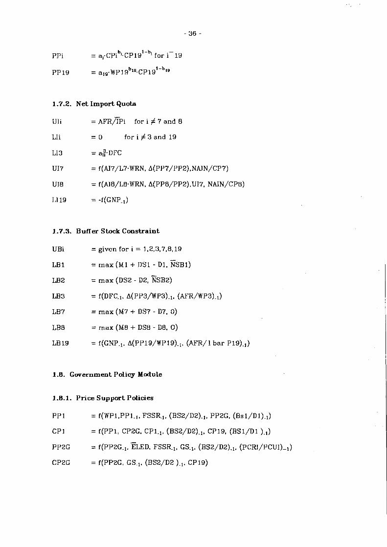
6.7.2. Net Import Quota The upper bounds of net import quotas of all commodities except for bovine

meat a n d q o r k a re se t with the maximum purchases by accumulated foreign reserves AFR/IPi. The lower bounds of net import quotas of all commodities except for coarse grains and nonagricultural commodities a r e zero. The upper bound of bovine meat import is set by a function of national income divided by consumer price of bovine meat, ratio of bovine meat production income per farmer over nonagricultural wage rate, and change in ratio of bovine meat pro- ducer price over rice producer price. The upper bound of pork import quota is affected by the upper bound of bovine meat irnport quota, real national income, ratlo of pork-production income per farmer over nonagricultural wage, and change in real pork price.

The lower bound of import quota of coarse grains which are used for non- protein feeds is needed for short-run stability of animal production. It is con- sidered to be proportional to the total animal demand for non-protein feed. Since the Japanese economy and daily life heavily depends on imports of petroleum and minerals, the lower bound of export exists and is considered to be a function of GNP.

6.7.3. Buffer Stock Constraint

The upper bounds of buffer stocks of storable commodities i = 1, 2, 3, 7, 8 and 19 in the llASA commodity list are given as exogenous. However, the lower bounds of buffer stocks of the storable commodities are explicitly expressed as functions of economic variables. Whenever positive excess supply of wheat Ml+DSl-Dl results, it is stored as buffer stock. From the viewpoint of national security, we believe that there is a rninimurn buffer stock of wheat NSBI which, for instance, can cover two mo_nthsl consumption of wheat. Therefore, if the minimum buffer stock of wheat NSBl is not satisfied, the government decides to import more wheat and/or to change the wheat production policy.

We also believe that the minimum buffer stock of rice NSBZ, for instance, two or three months' consumption of rice, is needed from the viewpoint of national security. Although rice is overproduced in Japan, the government has been taking measures to ban exporting rice except for sporadic cases. The lower bound of rice stock is defined as the maximum among the amount of excess supply anti the minimum buffer stock.

The lower bound of coarse grains for buffer stock is needed for short-run protection of animal production from the fluctuation of the world coarse grain price. Since animal production in Japan heavily depends on imported coarse grains, the lower bound d.epends on the total demand for non-protein feed. DFC-l, difference of real coarse grain producer price A(PP3/ WP3)_1, and real accunlu- lated foreign reserves (AFF1/WP3)_1. The lower bounds of buffer stocks of bovine meat and pork are equal to positive excess supplies of them, whenever the posi- tive excess supplies occur. The lower bound of nonagricultural commodities in inven1,ory depend.^ on GNP., , real producer price change A(P 19/ WP19)-1 and real

accumulated foreign reserves (AFR/IP19)-,.

6.8. Government Policy Module Government has various economic goals. These a r e (1) social stability, (2)

national security, (3) efficiency, (4) development and growth, and (5) coopera- tion with the res t of the world. Social stability may be regarded as a short-run goal and related t o equity and opportunity for employment. The rural-urban income gap, overpopulation in urban areas and high unemployment ra te may belong to the problems of social stability. National security is related t o national defense and uncertainty of domestic agricultural production and the international market . Energy and food storage and protection of domestic agri- cultural production are considered t o be measures for national security in the model.

Government investment is here considered to make contributions mainly t o efficiency, development, and growth. Construction of infrastructure, various kinds of research, and fostering key industries are some measures for efficiency improvement, development, and growth. Economic aid, forced purchase of over- produced wheat from certain countries, and income transfer t , ~ international organizations belong t,o the category of cooperation with the world. Income transfers from urban to rural areas SUBA, and rice producer prices PPZG and government investment in rural a reas IGA can be considered to be very effective for social stability. Government control of wheat and rice, PP1. CP1. PPZG. CPZG, MI, BS1 and BS2, import. quota and tariff r a t e s UI7, UI8, TR7 and TR8, can be considered to be very effective for national security. Government investment in the agricultural as well a s the nonagricultural sector IGA and IGN, and govern- ment capital stock KGA and KGN a r e t reated as measures for the inlprovement of production efficiency and as incentives t o economic activities. Tax policties affect the economic goals (1) t o (4) to various degrees. Econonlic aid is not t rea ted in the model.

6.8.1. Price Support Policies

The rice producer price plays a key role in the determination of tlie rice consumer price, and producer as well as consumer prices of wheat and. tobacco. The wheat producer price PP3. is a funct,ion of the wheat world price WP1, the previous year's wheat producter price PP1-l, the food self-sufficiency ra te FSS1Z- 1, the ratio of rice storage over rice consumption (BS2/D2)_l, t he rice pro- ducer price PP2G, and the ratio of wheat storage over wheat consum.pt,ion BSl/Dl. The wheat flour czonsumer price CP1 is determined by wheat producer price PP1, polished rice consumer price CPZG, previous year 's wheat flour- con- sumer p rice CP1-l, rat io of rice stock over rice consurnption (BSZ/D2)_1, consu- m e r price of nonagricultur-al. cornmodities CP19 representing polishing and mil- ling wheat, and ratio of wheat stock over wheat consumption BSl/Dl. Th.e determination of rice producer price PP2G depends on t.he previous year 's r ice producer price PPZG.l, c;lect,ion dummy ELED, food self-sufficiency ra te FSSR_l, government deficits GS, ratio of rice s tock over rice consum.pt;ion (BS2/D2).1. and ratio of per capita rural income over per capita urban income (PCRI/PCUI)_

Consumer price CPZG of polished rice is a function of rice pr-oducer price PPZG, government deficits GS-l, ratio of rice stock over rice consumpt.ion (BS2/D2)-1 and consumer price CP19 of nonagricultural commodities which represents polishing cost. Producer price P18T of tobacco is affected by the previous year's tobacco proclucer price 'l'18T1 and rice producer price PPZG. Tobacco consum.er price Cl8T is determined by tobacco producer price P3.8T, the previous year 's t,obacco consumer price ClST-,, ratio of governrrlent expen- ditures over government revenues GE/GR and t ime t,rend variable which

reflect.^ the lung cancer problem.

The wage ra te WRG for government er~lployees is determined by thc prt:vi- ous year 's wage ra te for government erriployces WRC-l and the previous year 's wage rate for nonagricultural production WRN_l. The time lag of these explana- tory variables implies wage rigidity.

6.8.2. Agricultural Production Policies

Income transfer t o agriculture SLTBA which is here called subsidies to agri- culture is determined by food self-sufficiency ra te FSSR_l, ratio of per capita rural income over per capita urban i n c o s e (PCRI/PCUI)-l, and ratio of urban population over total population (UPOP/TPOP)-l. Fallow payment per acre of paddy field is deterrnined by ratio of rice stock over rice consumption (BS2/D2).I, land rice-income productivity (PPZG-Q~/AZ).~, and the previous year 's rice acreage A2.1.

6.8.3. International Trade Policies

Tariff r a t e TRi depends on the previous year 's import-productior~ ratio (ML/ Qi).I, government expenditures-revenues ratio GE/GR, real accumulated foreign reserves AFR/TPI 9, and previous year 's tariff rate TRi-jl Import of wheat - MI is determined by real accumulated foreign reserves AFR/IP19, the previous year 's wheat production Ql-,, the previous year's ratio of rice stock over rice consumption, and the previous year's ratio of wheat stock over wheat corisump- tion. Import of t,obacco M18T is a function of real acr:umulated foreign reserves A F R / ~ P ~ ~ , GNP change AGNP, and the previous year's ratio of tobacco produc- tion over tobacco import (Q18T/M18T)-1.

6.8.4. Taxation Policies Nonagricultural personal t a x rate NPTX is determined by GNP growtll rate ,

real average government deficits during the last two years ( G S - ~ + GS_,)/(Z-GPI,), and election dummy ELED. Agricultural personal tax ra te APTX depends r!n GNP growth rate , real average government deficits during the last two years (GS_l + GS.2)/(2.GPL), previous year 's food self-sufficiency ra te FSSR-I, and nonagricul- tural personal tax ra te NPTX. The indirect tax r a t e imposed on consuriiptiol~ of sugar and sugar products denoted by IlXS is chanxed by the previous year 's sugar Indirect tax r a t e ITXS_I time trend variable t, and real average govern- ment deficits during the last two years (GS-1 + GS_2)/(2.GPL). The indirect t a x ra te imposed on alcoholic beverages denoted by ITXB is a function of ratio of government expenditures over government revenues GE/GR, the previousyear 's alcoholic beverage indirect tax ra te ITXEI.I, and time trend variable t. The indirect tax ra te imposed on nonagricultural commodities denoted by J'I'XN is determined by CNP growth ra te , ratio of inventory over production of nonagri- cultural comrnodit.ies BS19/Q19, and real average government deficits during the last two years (GS.I + GS-2)/(2-GPL). Finally, corporate t a x r a t e CTX is determined by CNP growth rate , ratio of inventory over production of nonagri- cultural coninlodities BS19/Q19, the previous year's retained earnings-gross profit ratio (RE/GP19)-l, and real average government deficits during the last

two years (GSJ + GS.,)/(Z.GPL).

7 . CONCLUDING REMARKS Japan joined IIASA's Food and Agriculture Program in January of 1980. The

purpose of this article is to show a mathematical framework for the Japanese agricultural model . JAM, which is suitable for IIASA's World Model Linkage. The model is designed to represent the Japanese economy with the emphasis on the agricultural sector. So far, the data bank necessary for the estimation of the model JAM has been made neither iri IIASA-nor in the University of Tsukuba. I t is planned tha t we s t a r t making the data bank in the University of Tsukuba this September. Then, the estimation and economic simulation will be made. Finally, I would like to mention that JAM may be modified later when we s t a r t estimating JAM.

A P P E N D I X 1

1. MATI-IEMATICAL FRAMEWORK FOR T H E J A P A N E S E AGRICULTURAL MODEL

1.1. M a r k e t C l e a r a n c e and Social A c c o u n t M o d u l e

1.1.1. D e m a n d f o r C o m m o d i t i e s

= (RT1 + ~ ~ l ) / a : + F1 + BS1

= (RTZ + UTZ + I D Z ) / ~ ~ + FZ + BS2

= RT3 + UT3 + F 3 + ID3 + B S 3

= RTi + UTifor i = 4 ,6 ,9 ,10 ,14 ,15 ,16 ,17 ,10

= RTi + UTi + BSi for i = 7 , 6

Refers to (3 .4) Animal Consumption

= R T l l + U T l l + w , " . ~ 1 1 ~ + ID11

= RT1Z + UT1Z + W,". I~ZG

= RT13 + UT13 + ID13

= RT19 + UT19 + GC + IG + IA + IN + IH + ID19 + BS19

1.1.2. Domestic Supplies of Commodities

DSi = Qi-, + BSi-I for i = 1,2

DSi = Q l l + BSi-, for i = 3,7,8,19

DSi = Qi-, f o r i = 4,5,6.9,10.11,12,13,15,16,17,18

DS14 = 0

1.1.3. Excess Demands for Commodities

Mi = Di - DSi

1.1.4. Agricultural, Farm and Rural Incon~es

C Ii

CIi

C I

A1 i

A1

FARI

FISI

FOR1

DAA

AGIN

FI

N AFI

DFI

R1

D RI

= PPi-Qi-l - ~ ~ 1 9 . a : ~ ~ i . . ~ for i = 6,11,12,15,16,17,1f3

= PPi-Qi-l - ~ ~ 1 9 . ( a , ' ~ . ~ i _ ~ + a L 9 . ~ ~ i - , ) for i = 1,2,3

= CIifor i = 1,2,3,6,11,12,15,16,17,18

= PPi-Qi_l - C~19.a:~.Qi_~ - CP5.FDi-l-Qi-l for i = 7,f3,9,10

= AIi for i = 7.8,9,10

= C I + A I

= PP13-Q13-1 - CP19.a{!.~13-~

= PFOR.QFOR.l - C P ~ ~ . ~ ~ ' , ~ . Q F O R _ ~

= f(KFAR + KFIS + KFOR)

= FARI + FISI + FOR1

= AGIN + NAFI + ITOF + DIVF + ARPZ-AR2

= WRN.(LNAR - LGR) + WRG-LGR

= (FI - DAA)-(1-APTX) + DAA

= FI + SUBA

= DFI + SUBA

DRZ-I1 = DRl/NRH

PDI i l = DRI/RPOP

F'AIF = FARI/LFAR

F l I F = F I S I / L F I S

F O l F = FORI /LFOR

PCAI = AGIN/(LAR - LNAR)

P C F I = F I / R P O P

1.1.5. Urban Income

UWI = WRN-(ENAL - (LNAR - LGR)) + WRG.LGU

U I = UWI + DIVU + ITOU

DU 1 = U I . ( l - NPTX)

DUHI = DUI/NUH

P D U I = D U I / U P O P

1.1.6. Nonagricultural Revenue

G P 19 = NC 1 9 .NQ19-1- (1 - ITXN) + ITON - WRN-ENAL - DAN

DAN = f(KN, KURN)

DIVI = ~ ( G P I S )

RE = G P 1 9 . ( 1 - CTX) - DIVI + DAN

DlVF = ~ ~ . D I V I

DIVU = DIVI - DIVF

1.1.7. Gwernment Revenue and Expenditure

+ CP6.116.1TXS + C P 16.D 16.II'XR

+ CPl9-QI9- ITXN + ~ T R ~ - M ~ . w P ~ + GP19.(:TX + ITOG

GE = CPl9 . ( IG + CG) + P P I . Q l + WP1.Ml

+ PP2GeQ2G + P18T-Q18T + W1BfI'.M18T

+ SUBA + ARP2.AR2 + WRG.LGOV

1.1.8. Gross National Product, National Income and General Price Level

GNP = ~ P P ~ . Q ~ - ~ / G P L

GPL = x (Qi_ l /C Q ~ - , ) . P P ~

NAIN = AGIN + NP19.NQ19

1.2. Population. Labor Availability. Household, and Land Availability Module

1.2.1. Rural and Urban Population

RPOP = POP-,, (PDRI/PDUI)-1, IGA-1, (UPOP/'*OP)-I)

7

UPOP = TPOP - RPOP

1.2.2. Labor Availability

LA R = ~ ( R P O P , (REFH/DRHI)-,, T)

LFAR = f(LAR, KFAR/LAND, (FAIF/WRN)-i)

LFlS = ~ ( L F I S - ~ , KFIS, (FIIF/WRN)-l, THMD)

LFOR = f(LF0R-1, KFOR, (FOIF/WRN)-I)

LNAR = IAR - LFAR - LFIS - LFOR

LAU = f (UPOP, (DEFH/DUHI)-,, T)

LNAP = IAU + LNAR

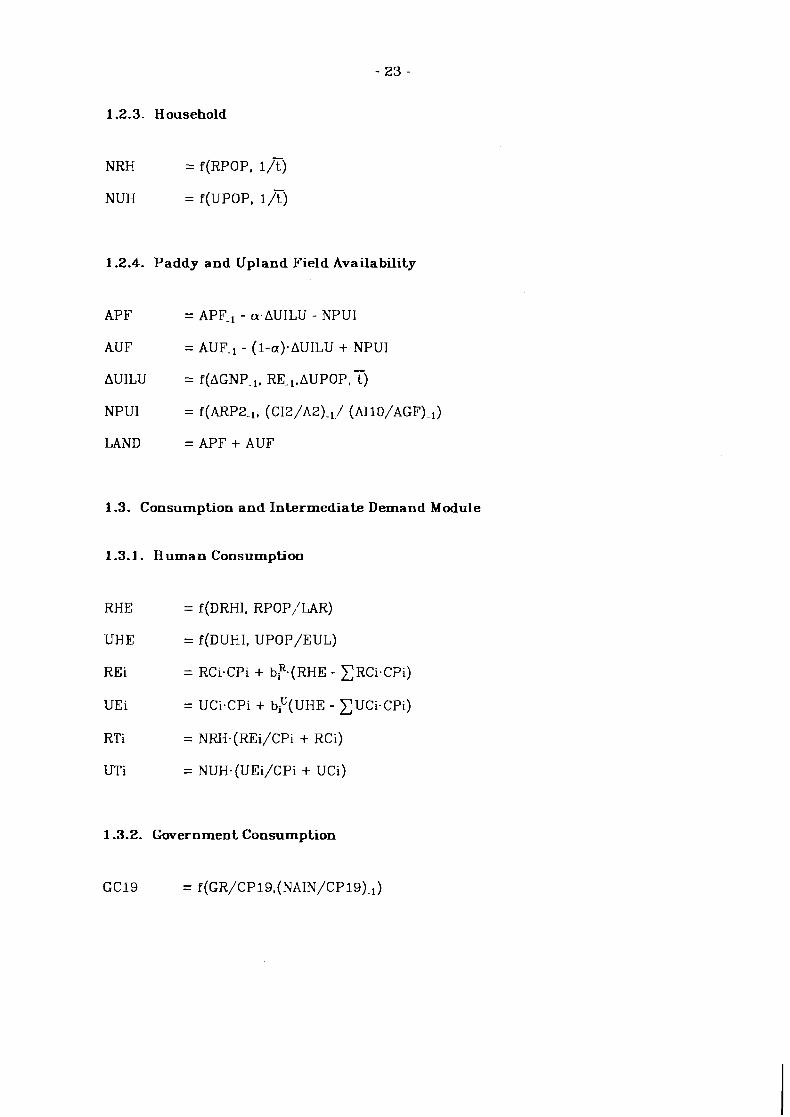
1.2.3. Household

NRH = f(RPOP, l/T)

NU14 = f(LTPOP, l /y )

1.2.4. Paddy and Upland' Field Availability

A P F = APF-1 - a.AUILU - NPUI

AUF = AUF-1 - (1-a).AUILU + NPUI

AUILU = ~ ( A G N P - ~ , R E ~ . A U P O P , T )

NPUI = f(ARP2-1, (C12/A2)_1/ (A1 10/AGF).l)

LAND = A P F + AUF

1.3. Consumption and Intermediate Demand Module

1.3.1. Human Consumption

RHE = ~ ( D R H I , RPOP//LAR)

UH E = ~ ( D L ~ H I , UPOP/EUL)

REi = RCi-CPi + ~ F . ( R H E - Z R C i . C p i )

UE i = UCi-CPi + ~ ~ ( U H E - Z U C i - C P i )

RT1 = NRH-(REi/CPi + RCi)

UTi = NUH.(UEi/CPi + UCi)

1 -3.2. Gwernment Consumption

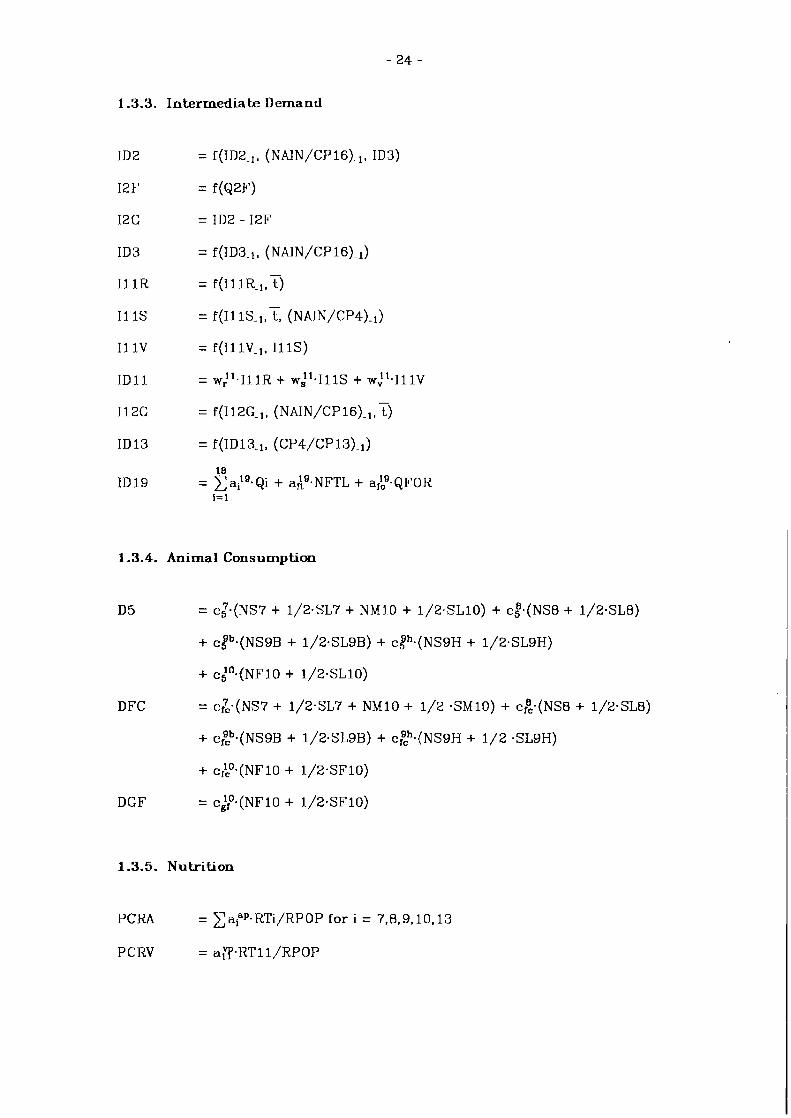
1.3.3. Intermediate Demand

1.3.4. Animal Consumption

D5 = C;.(NS~ + 1/2.SL7 + NM30 + 1/2-SL10) + c:-(Ns~ + 1/2.SLB)

+ c { ~ - ( N s ~ B + 1/2.SL9B) + c:~.(Ns~H + 1/2.SL9H)

+ C;O.(NFIO + I /~-SLIO)

DFC = c & - ( N s ~ + 1/2.SL7 + N M l O + 1/2 .SM10) + cfa,.(Ns8 + 1/2-SL8)

+ cEb . (Ns9~ + 1/2*SL9B) + c ~ ~ - ( N s ~ H + 1/2 .SL9H)

+ cl',O.(NF10 + 1/2*SF10)

DGF = c,'iO.(NFlo + 1/2.SF10)

1.3.5. Nutrition

PCRA = zaiaP.RTi/RPOP for i = 7,8,9,10, 13

PCRV = a%-HT1 l/RPOP

PCRT

PCRC

P C R F

PCRK

PCUA

PCUV

PCUT

PCUC

P C U F

PCUK

PCAP

PCVP

PCTP

PCC

= RA + PCRV

= z a F . R T i / R P O P f o r i = 1 , 2 , 3 , 6

= ~ ~ / . R T ~ / R P O P f o r i = 4 ,7 ,8 .9 ,13

= z a i C " ' - ~ T 1 / ~ ~ O ~

= za?p.UTi/LTPOP f o r i = 7 ,8 ,9 , lO, 13)

= a n . U T 1 l / U P O P

= PCUA + PCUV

= z a F . U T i / U P O P f o r i = 1 , 2 , 3 , 6

= ~ ~ ~ U T ~ / U P O P f o r i = 4 , 7 , 8 , 9 , 1 3

= z a i C " ' - U T i / U ~ O ~

= z a ? P - ( R T i + UT~)/??OP f o r i = 7 . 8 , 9 , 1 0 , 1 3

= a n - ( R T 1 1 + UTII)/TPOP

= PCAP + PCVP

= z a ? - ( ~ T i + UT~)TPOP f o r i = 1 . 7 , 8 , 9 , 1 3

1.4. A g r i c u l t u r a l P r o d u c t i o n M o d u l e

WHR = f((KFAR + KFIS + KFOR)/(LFAR + LFIS + LFOR),(PDRI/CP2)-,)

NFTL = f(NFTL-I, (CI/PP~)-~),(PNF/PP~)-~)

PNF = ~ ( N F T L , PNF-I, ~ ~ 1 9 )

1 A.1. W h e a t P r o d u c t i o n

Q1 = f(A1. NF1, K1, KGA, L1, 5 1 1 , T )

1.4.2. Hulled Rice Production

= f (ARP2 -1, (BS2/QZ)-l)

= A P F - ARZ

= NFTL - N F 1 - N F 3 B - N F 3 R - NF3C

= KFAR - K 1 - K3B - K3R - K3C - K6B - K6C - K 7

- KB - K g - K l O - K 1 1 - K 1 2 - K 1 5 - K 1 7 - K G F

= WHR.LFAR - L 1 - L3B - L3R - L3C - L6B - L6C - L 7

- LB - L 9 - L l O - L 1 1 - L 1 5 - L 1 7 - LGF

= f(A2, NFZ, KZ, KGA. L2, i 1 2 , T )

= P ( ( P P ~ F / P P Z G ) - ~ , (BS2/Q2)-l)

= Q 2 - QZF

= (Q2G.PP2G + Q2F*PPZF) /QZ

1.4.3. Production of Coarse Grains (Barley, Rye and Oats, and Corn)

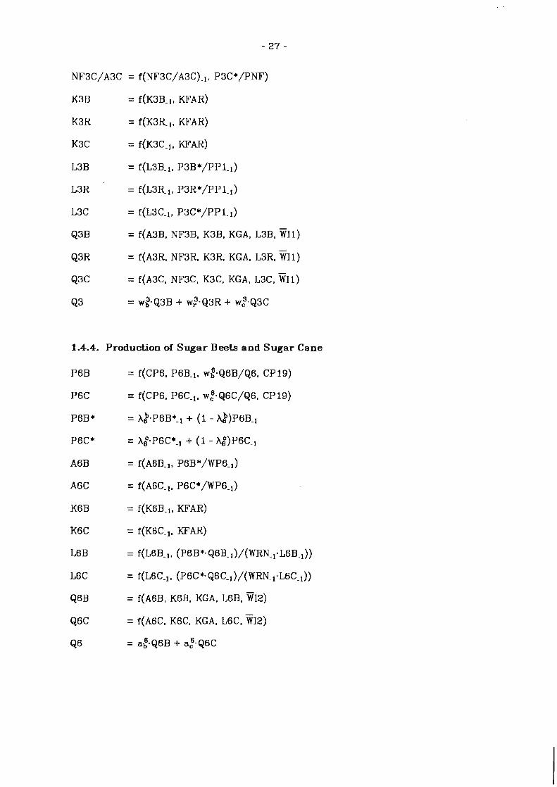
NF3C/A3C = ~ ( N F ~ c / A ~ C ) . , , P3Ce/PNF)

K3B = f ( ~ 3 B - 1, KFAR)

K3R = f (K3R- KFAR)

K3C = f(K3C-,, W A R )

L3B = f(L3B.1, P3B*/PP1-1)

L3R = f(L3R-1, P3R*/PP1-1)

L3C = f(L3C-1, P3C*/PP1-1)

Q3B = f ( ~ 3 B , NF3B, K3B. KGA, L3B, W11)

Q3R = f(A3R, NF3R, K3R, KGA, L3R, i l l )

Q3C = f(A3C, NF3C, K3C, KGA. L3C, i 1 1 )

63 = w , 3 - ~ 3 ~ + W:-Q~R + ~ 2 . 6 3 ~

1.4.4. Production of Sugar Beets and Sugar Cane

= f(CP6, P6B-1, w ~ - Q ~ B / Q ~ , CP19)

= f(CP6, P6C-I, W:.Q~C/QG, CP19)

= x & P ~ B * - ~ + ( I - A ~ ) P G B - ~

= A ~ - P 6 C * - l + (1 - Ag)P6C.l

= ~ ( A G B - ~ , P ~ B * / w P ~ _ I )

= ~ ( A G C - ~ , P6C*/WP6-1)

= f(K6B- 1. KFAR)

= I ( K ~ C . ~ , KFAR)

= f(L6B-i, (P6B*. Q6B-l)/(WRN.l.L6B-l))

= ~ ( L ~ C J , (P6C*.Q6C-1)/(WRN_l.L6C-l))

= f(A6B, K6B, KGA. L6B. F12)

= f(A6C, K6C, KGA, L6C, W12)

= a;.Q6B + a , 6 - ~ 6 ~

1.4.5. Production of Bovine Meat and Milk

N7

PNF5

B?

PP?*

SL?

NS?

E7

N10

B10

SF10

NFlO

SMIO

NLI 10

Q 7

Q l O

K?

L 7

K10

L10

= (1 + B7).NS7_,

= dl.PNPF + d2,CP5

= f(PP7-l/PP8-l, P P ~ - ~ / P N F ~ . I . )

= A7.PP?*-l + (1 - A ~ ) . P P ? - ~

= f(N7, PP?*/PPB_~)

= N7 - SL7

= f(T)

= (1 + ~ / Z . B ~ O ) ~ N F ~ O - ~

= f(PP10-l/PP10-2, Q Q G F / N F ~ O - ~ , ~ )

= f(N10. PP7_l/PP10-1, QQGF)

= N10 - SF10

= f(NM10-, + 1/2.BlO-NF10, PP?-1/PP8_1)

= NMIO-I + 1/2.B10-NF10-1 - SMlO

= E7.(SL? + a,;SF10 + SM10)

= f(N10 - 1/2.SF10, QQGF/NF1O_l)

= a z . ( ~ 7 + NM10)

= ~Y-(N? + NM10)

= a i O - N ~ 1 0

= a I1O .~~10

1.4.6. Production of Pork

N8 = (1 + B8).NS8-1

PPB* = h,-PP8*-l + (1 - A ~ ) . P P ~ - ~

B8 = ~(PPB*/CPS-~,T)

SL8 = f(N8. PPB* /CP~-~ )

NSH = N8 -SLB

EB = f(F)

88 = EB-SLB

KB = af-Nt3

LB = ale-NB

1.4.7. Production of Poultry and Eggs

1.4.8. Production of Starchy Roots, Soybeans, and Vegetables

P l l R = f ( ~ ~ 1 1 , P 1 l R _ l , ~ , ' ~ - Q l l ~ / Q l l )

p l l s = ~ ( P P I I , PI IS-^, ~ , l ' . ~ i i s / ~ i i )

p l l v = (~1 '1 1 . ~ 1 1 - P I I R . Q ~ ~ R - ~ l l s . ~ l l s > / ~ l l v

P 1 l R *

P1 1s''

PlIV*

A l l R

A1 lS

A1 l V

Q l l R

QllS

Q l l V

K11

L11

Qll

1.4.9. Production of Grapes and Other Fruits

P 12G = f(PP12, P12G-,, w 1 2 - ~ 1 2 ~ / ~ 1 2 )

Pl2F = (PP12.Ql2 - P12G.Q12G)/Q12F)

P12G* = h&.P12G*-l + (1 -A& ) . P I ~ G - ~

PlZF* = A : ~ . P ~ ~ F * - ~ + (1 -hi2 ) . ~ 1 2 ~ - ~

A12G = f(A1ZG-,, P 12G*/P12F-1)

A12F = f(A12F-1, P12F*/P12G-1)

Ql2G = f(A12G, AQ12G-l, W12)

QlZF = f(AlZF, AQ12F.1, W12)

K12 = ~ E - Q ~ z G + a g . 8 1 2 ~

L12 = a l ~ z - ~ 1 2 ~ + ai2.Q12F

Q l 2 = W,'~-QIZG + W;~-QIZF

1.4.10. Production of Fish

Q13 = ~(WHR-LFIS, KFIS, THMD)

1.4.11. Production of Tea

P 1 5 T = f (CP15, P15T-1, ~ ~ ~ . ~ 1 5 ~ / ~ 1 5 )

P 15T* = A : ~ . P ~ ~ T * - ~ + (1 - ~ : ~ ) . P 1 5 T - l

A15T = f(A15T-1, P15T*/WP 14-1)

Q l 5 T = f(A15T, W12)

K15 = s2 f .Q l5

L15 = s ] : ~ . Q I ~

Q15 = w < ~ Q ~ ~ T

1.4.12. Production of Silk Cocoons

1.4.13. Production of Tobacco and Igusa Plants

1.4.14. Production of Woods

PFOR = ~(PPIS , W,',~.QFOR/QIS)

QFOR = f(WHR-LFOR. KFOR + KGA)

1.4.1 5 . Production of Green Feed

ACF = F(AGF-~, (PPIO/PPZ).,, ARPZ)

QGF = F(AGF)

KGF = ~#'.QGF

LGF = a f t ~ C F

1.4.16. Production of Joint Products and processed Foods

1.4.17. Productitw of Now protein and Green Feed

QFC = ~ , ' ~ . ( l - a: ) . (RTl + UT1) + wd-F bar 1

+ w,Zb-(1 - azb ).(RT2 + UT2 + 1 ~ 2 ) / ( l / a : - 1 )

+ W$F' b a r 2 + ~ 2 . ~ 3 + wtb-( 1 - a ; ) . Q 6 ~

+ wZc.(l - ~ Z ) . Q ~ C + w , " - a P . ~ l l ~

QQGF = a;MEAD + Q G F

1.4.18. Food Self- sufficiency Rate

F S S R = z C ~ i . Q i / C C P i - D i

1.5. Nonagricultural Production and Government Employment Module

1.5.1. Nonagricultural Labor, Employment, Wage Rate. Capital Use Rate, and

Production

ENAL

E U L

WHN

U E

KURN

KAUN

TWHN

WRN

N Q l 9

Q19

N P 1 9

= f(WRN/NP19, KN/LNAP, ENAL.1)

= ENAL - (LNAR - LGR)

= ~ ( ( K N + KGN)/LNAP. WHN~~,(UEFH!~NUH)~~/UPOP~~,~)

= LNAP - ENAL - LGOV

= f ( ( N ~ 1 ~ / K N ) - I / ( N Q 19/KN)-,, ( B S 19 /Q 19)-i , IG/IG-l)

= KURN-KN

= WHN-ENAL

= ~ ( ( N P 19-NQl9/ENAL)_l , WRN-1)

= ~ ( ~ ) . K A u N ~ - T w H N ' - ~

= W : & N Q I ~ + W/:.QFOR

= ( P P 1 9 . Q l 9 - PFOR.QFOR) /NQl9

1.5.2. Government Employment

LGOV = f(LNAP, WRG/WRN)

LGR = a g r LGOV

LGU = (1 - agr) .LGOV

1.6. Investment and Capital Formation Module

1.6.1. Investment

I G = f((NAIN/GPL)_l, IG-1, (GR/GPL)_l)

IG A = ~ ( I G A - ~ . FSSR-,, (PCAI/PCUI).,)

IGN = IG - IGA

IN = f (RE/CP 1 9 , C(4- i ) .Q19- , /6 , C(4-i)-KURN-,/G, IR, KN-1,

C ( 4 - i ) m ~ P 1 9 - i / ( 6 C P I~ -~ .KN- , ) )

I A ! = f ( C ( ~ - ~ ) - F S S R - ~ / S , C ( ~ - ~ ) . I G A - ~ / G , C (4-i).RE-i/(6.CP 1 g-i.(KFAR

+ K F I S + KFOR)-~), IR, (KFAR + K F I S + KF0R)- , )

I F I S = f(C (4-i)-Q 13-,/6. IFIS-l, (PFII/PFAI)-l , KFIS- l )

IFOR = f ( C ( 4 - i ) .QFORi/6 . IFOR-1, (PFOI/PFAI).l, KFOR1)

IFAR = IA - I F I S - IFOR

RS = DRI - RHI-NRH

U S = DUI - UHEaNUH

GS = GR - G E

IR = ~ ( G N P - ~ , ~ 1 9 . 1 )

IH = (RS + U S + G S + R E ) / C P 1 9 - (IG + IN + IA)

1.6.2. capital Formation

KFAR = KFAR-1 + IFAR-1 - DFAR

KFI S = KFIS-1 + IFIS-, - DFIS

KFOR = KFOR-1 + IFOR-, - DFOR

XN = KN-1 + IN-1 - DN

KGA = KGA-1 + IGA-1 - DGA

KGN = KGN-1 + IGN-1 - DGN

KH = KH-1 + IH-1 - D H

1.6.3. Depre ,iaLion oi Capital

DFAR = f(KFAR.l. GNP-1)

~ F I S = ~ ( K F I S - I , GNP-I}

DFOR = ~ ( K F O R - ~ , G N P . ~ )

D N = ~ ( K N - ~ , G N P . ~ )

DGA = ~ ( K G A - ~ , GNP.~)

DGN = f ( 7 : ~ ~ . l , GNP.,)

TIH = f(l:Y-l)

1.7. International Trade, Price Determination. Net Import Quota, and Buffer

Stock Constraint Module

1.7.1. International Trade and Price Determination

FXR = ~ ( ( G N P / ~ G N P ) _ , , ( A F R / W P ~ ~ ) - ~ , FXR-I)

AFR = AFR-I + FR - F R = - X T p i a ~ i

ITOC, = ~ ; ~ R . F X R

ITOF * ar.TR. F'XR

ITOU = ~;FR-FXR

ITON = ( 1 - ag-al-a , ) .F~-FXR

WPi = ~;-FXR%'~+ b j g i . F ~ R . I P 1 9 for i # 2 and 19

WP 19 = a ~ 9 . ~ ~ ~ ~ 1 9

T P i = a$-(1 + TRi).WPi f o r i # 1 and 2

CPi = TPi + LUi - LLi for i f 1 and 2

LUi.(UIi - Mi) = 0

I,Li.(Mi - LLi) = 0

LUi-(BSi - LBi) = 0

LLi-(UBi - BSi) = 0

b. PPi = ai.CPi ' - ~ ~ 1 9 ' - ~ ' for i- 19

PP 19 b = a l e - w ~ 1 9 1g .~~191-b1e

1.7.2. Net Import Quota

LTIi = AFR/TP~ for i # 7 and 8

LI i = 0 for i # 3 and 19

L13 = ~ $ D F c

U17 = f(AI7/L7*WRN, A(PP7/PP2),NAIN/CP7)

UI8 = f(AI8/L8-WRN. A(PP8/PP2),U17, NAIN/CPB)

LI 19 = -f(GNPJ)

1.7.3. Buffer Stock Constraint

UBi = given for i = 1.2,3,7,8,19

LB 1 = max (MI + DSI - DI, NSBI)

LBZ = max (DS2 - D2, NSBZ)

LB 3 = f(DFC-1, A(PP3/WP3)-1, (AFR/WP3).1)

LB7 = max (M7 + DS7 - D7, 0)

LB8 = max (M8 + DSB - D8, 0)

LB 19 = f(GNP-l, A(PP19/WP19)-,, (AFR/ 1 bar P19)-1)

1.8. Gwernment Policy Module

1.8.1. Price Support Policies

PP 1 = f(WP1,PPl-1, FSSR-1, (BS2/D2)-1, PPZG. ( B s ~ / D ~ ) _ ~ )

CP 1 = f(PP1, CPZG, CPl-i, (BSZ/D2)_1, CP19, (BSl/Dl

PP2G = f(PPZG-I, ED, FSSR-1, GS-1. (BSZ/D2)-1, (PCRI/PCUI)-1)

CP2G = ~(PPzG, GS.1, (BS2/D2 )-,. CP19)

P 1 8 T = ~ ( P I B T - ~ , P P Z G )

c IBT = f ( ~ 18T, CIBT-,. G E / G R ~ )

WRG = f(WRG-1, WRN-1)

1.8.2. Agricultural Production Policies

SUB A = ~(FSSR-I, (PCRI /PCUI)_~ , (uPoP/?;PoP)-,)

ARP2 = f((BS2/D2)-, , ( P P ~ G - Q ~ / A ~ ) . ~ , A2-1)

1 3.3. International Trade Policies

TRi = f((Mi/Qi)-l, GE/GR, AFR/TPIS, TRL1) f o r i = 6 , 7 , 8 , 1 0

M1 = ~(AFR/TP 1 9 , QZ-,, ( B S Z / D Z ) _ ~ , ( B S l / D I ) .~)

M l R T = ~(AFR/TP 19, AGNP, ( Q 1 8 ~ / M 1 8 ~ ) - ~ )

1.8.4. Taxation Policies

NPTX = ~(GNP, (GS- I + GS-2) /~ .GPL, ELED)

APTX = ~ ( G N P , (GS., + G S - 2 ) / ~ - ~ ~ ~ . FSSR-1, NP'I'X)

ITXS = ~ ( I T X S - ~ . T (GS-1 + GS-,)/Z.GPL)

ITXB = f(GE/GR, ITXBJ, T)

ITXN = ~ ( G N P , ~ S 1 9 / Q 1 9 , (GS-I + GS-~)/Z.GPL)

CTX = ~ ( G N P , B S 19/Q 19. ( R E / G P ~ S ) - ~ , (GS., + GS-z)/Z.GPL)

APPENDIX 2

VARIABLE NOTATIONS

A No te o n N o t a t i o n s

1. An endogenous variable which is not a policy 7-ariable does not have any hat

or bar over its notation, e.g., PP7, Q3, FI.

2. An endogenous variable which is a policy variable has a hat over its nota-

tion, e.g.. PP2G, ITXS, TR7.

3. An exogenous variable has a bar over its notation, e.g., $11, FLED,.

4. The time trend variable is expressed asT.

5. A lagged variable has a subscript with a minus sign, e.g., GNP-2. PPl-e.

6. An expected price variable has an asterisk a t the right-hand side of its nota-

tion, e.g., PPl*, PPB*.

7. Small letters of the alphabet and Greek letters are coefficients to be

estimated.

8. GKP = (GNP - GNP-l)/GNP.l

9. AGNP= GNP - GNP-1

10. ( B S ~ ~ / Q I ~ ) _ ~ = BS19-1/Q19-1

r~ P 'IX

Ali

AGIN

ARP2

AR2

AFR

Ai

A3B

A3R

A3C

A6B

A6C

A1 l R

A 1 l S

A 1 l V

A12C

A12F

A15T

A17M

A18T

A181

AGF

APF

AGS

ARS

AUS

Agricultural personal tax rate

Animal (production) income of animal i

Agricultural Income

Rice acreage reduction unit subsidy per acre

Acreage of paddy field reduced by rice acreage reduction

policy

Accumulated foreign reserves in terms of 1970 US dollars.

Acreage of crop i

Acreage of barley

Acreage of rye and oats

Acreage of corn and other cereals

Acreage of sugar beets

Acreage of sugar cane

Acreage of s tarchy roots

Acreage of soybeans

Acreage of vegetables

Acreage of grape

Acreage of other fruits

Acreage of tea

Acreage of mulberry

Acreage of tobacco

Acreage of igusa

Acreage of green feed

Acreage of total paddy fields

Accurnulated governmer~t sav ngs

Accumulated ru ra l savings

Accurnulated urban savings

AUF

CTX

CPi

Cli

CI

DAA

DAN

DFI

DRI

DRHl

DUHl

DUI

DIVI

DFIS

DFOR

DN

DGA

DGN

DH

DSi

- ELED

Acreage of total upland fields

Buffer stock of commodity i

Net birttr ratc of animal i

Corporate income tax rate

Consumer price of commodity i

Crop income of crop i

Consumer price of tobacco

Consumer price of polished rice sold by the government

= XCIi

Depreciation allowances for agricultural capital

Depreciation allowances for nonagricultural capital

Disposable farm income

Disposable rural income

Disposable rural household income

Disposable urban household income

Disposable urban income

Dividend

Total demand quantity of commodity i

Depreciation of farming capital

Depreciation of fishery capital

Depreciation of forestry capital

Depreciation of capital in nonagriculture

Depreciation of government capital in agriculture

Depreciation of government capital in nonagriculture

Depreciation of housing

Domestic supply quantity of commodity i

Election dummy

ENAL

F1

FISI

FDi

FSSR

FIIF

FOIF

D[R

GS

- GROR

GNP

GP 19

TTXS

ITXN

ITXB

Employed nonagricultural labor (persons)

ProducLion quantity of commodity i from animal i e.g., hogs jpork

Employed urban labor (persons)

Production quantity of poultry from broilers

Farm income

Fishery income

Forestry income

Feed intake per head of animal i

Farming income

Food self-sufficiency ra t e

Farming income per farmer

Fishery income pe r fisherman

Forest,ry income per forestry worker

Foreign exchange ra t e

Quantity of commodity i consumed as feed

Foreign reserves (or foreign deficits) in t e rms of 1970 US$

Government revenue

Government expenditures

Government savings (on balance)

Government ruling and opposition party member ratio

Gross national product

Government consumption quantity of commodity 19, i.e.,

nonagricultural commodity.

Cross profit of nonagricultural production

Indirect tax ra te imposed on sugar

Indirect tax ra te imposed on nonagricultural commodity

Indirect tax ra te imposed on alcoholic beverages

ITOG

IGA

IG

I A

IGN

IN

IH

IDi

ITOF

ITOU

ITON

- IPi

Net income transfer from overseas t o government

Government investment in agriculture

Total government investment

Investment in agriculture (private)

Government investment in nonagriculture

Investment in nonagriculture (private)

Investment in housing

Intermediate demand quantity of commodity i

Net income transfer from overseas t o farmers, fishermen,

and forestry workers

Net income transfer from overseas t o urban dwellers

Net income transfer from overseas t o nonagricultural

corporations

IIASA world price of commodity i (pr ices in t e rms of

1970 US$)

Intermediate demand quantity of free-market rice used

for production of sake liquor

Intermediate demand quantity of government-controlled rice

used for production of sake liquor

Intermediate demand quantity of s ta rchy roots used for

production of alcohol

lntermediate demand quantity of soybeans used for pro-

duction of vegetable oil (and protein-feed cake)

Intermediate demand quantity of vegetables (rape seeds,

sunflower seeds, sesame seeds, e tc . ) used for production

of vegetable oil.

Intermediate demand quantity of g rape used for production

IR

KN

KFAR

KFIS

KFOR

KURN

Ki

K3B

K3R

K 3 C

K6B

K6 C

KGF

KAUN

KGA

KGN

KH

LNAF

LFAR

LFIS

LFOR

Li

of wine

Intermediate demand quantity of fish used for production

of fish oil (and fish meal)

Intermediate demand quantity of nonagricultural commodities

used for agricultural production

Real interest r a t e

Capital in nonagricultural sector

Capital for farming

Capital for fishery

Capilal for forestry

Capital use ra te of capital in nonagricultural sector

Capital used for production of commodity i

Capital used for production of barley

Capital used for production of rye and oats

Capital used for production of corn and other cereals

Capital used for production of sugar bee ts

Capital used for production of sugar cane

Capital used for production of green feed

Capital actually used for nonagricultural production

Government capital in agriculture

Government capital i n nonagriculture

Housing capital

Labor for nonagricult.ura1 production from rural a reas

Labor for farming. i-e., cropping and animal production (persons)

Labor for fishery (persons)

Labor for forestry (persons)

Labor used for the production of colnmodity i (man-days)

L3B

L3R

L3C

L6b

L6C

LGF

LAR

LAND

LAU

LNAP

LLi

LI i

LB i

LGOV

LGR

IJGU

Mi

M 18T

M1

MEAD

NAFI

NRH

Labor for barley (man-days)

Labor for rye and oats (man-days)

Labor for corn and other cereals (man-days)

Labor for sugar beets (man-days)

Labor for sugar cane (man-days)

Labor for green feed (man-days)

Labor availability in rural area -(persons)

Sum of acreage of paddy and upland fields

Labor availability in urban areas (persons)

Labor availability for nonagricultural production

Lagrangean multiplier of constraint imposed on the lower

bound of import of commodity i and/or constraint

imposed on the lower bound of buffer stock of commodity i

Lagrangean multiplier of constraint imposed on the upper

bound of import of commodity i and/or constraint

imposed on the upper bound of buffer stock of commodity i

Lower bound of net import quota imposed on commcdity i

Lower bound of buffer stock of commodity i

Labor employed by the government

Labor employed from rural areas by the government

Labor employed from urban areas by the government

Net import of commodity i

Net import of tobacco

Net import of wheat

Acreage of meadow and pasture

Nonagricultural income

Number of rural households

NUH

NPTX

Ni

NSi

NFlO

N M l O

N9B

N9H

NS9B

NS9H

NFTL

NFi

NPUI

NAIN

PPi

PDRl

PDUl

PP 2G

PFOR

PNF

PPi*

PP2F

P3B

P3R

P3C

J33B*

P3R*

Number of urban households

Nonagricultural personal tax ra te

Number of animal i

Number of animal i surviving a t the end of a year

Number of cows surviving a t the end of a year

Number of bulls surviving a t the end of a year

Number of broilers raised during a year

Number of hens raised during a year

Number of broilers surviving a t the end of a year

Number of hens surviving a t the end of a year

Total quantity of nitrogen fertilizer

Nitrogen fertilizer quantity applied to crop i

Net incremental acreage from paddy to upland field

National income

Producer price of commodity i

Per capita disposable rural incorne

Per capita disposable urban income

Producer price of (hulled) rice bought by the government

Producer price of wood

Price of nitrogen fertilizer

Expected producer price of commodity i

Producer price of free-market (hulled) rice

Producer price of barley

Producer price of rye and oats

Producer price of corn and other cerea s

Expected producer price of barley

Expected producer price of rye and oats

P3C*

P6B

P6C

P6B*

P6C*

P 9B

P9E*

P9B*

P 9E

P l l R

P 11s

P l lV

P l l R *

P1 IS*

Pl lV*

P 1 ZG

P 12F

PlZG*

PlZF*

P15T

P15T*

P17C

P17C*

PCRA

PCRV

I'CRT

lJCRC

Expected producer price of corn and other cereals

Producer price of sugar beets

Producer price of sugar cane

Expected producer price of sugar beets

Expected producer price of sugar cane

Producer price of broilers (and hen poultry meats)

Producer price of eggs

Expected producer price of broilers (and hen poultry meats )

Expected producer price of eggs

Producer price of starchy roots

Producer price of soybeans

Producer price of vegetables

Expected producer price of s tarchy roots

Expected producer price of soybeans

Expected producer price of vegetables

Producer price of grape

Producer price of other fruits

Expected producer price of grape

Expected producer price of other fruits

Producer price of t ea

Expected producer price of t ea

Producer price of silk cocoons

Expected producer price of silk cocoons

Per capita animal protein intake in rura l areas

Per capita vegetable protein intake in rural areas

Per capita protein intake in rural areas

Per capita carbohytlra.tes intake in rural areas

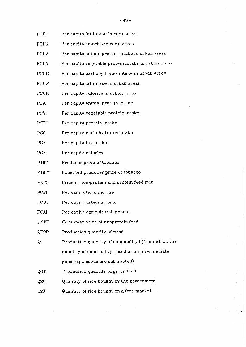
PCRF

PCRK

PCUA

PCUV

PCUC

PCUF

PCUK

PCAP

P CVP

PCTP

PCC

PCF

PCK

P18T

P lBT*

PNFS

PCFI

PCUI

PCAI

PNPF

QFOR

Qi

Per capita fat intake in rural areas

Per capita calories in rural areas

Per capita animal protein intake in urban areas

Per capita vegetable protein intake in urban areas

Per capita carbohydrates intake in urban areas

Per capita fat intake in urban areas

Per capita calories in urban areas

Per capita animal protein intake

Per capita vegetable protein intake

Per capita protein intake

Per capita carbohydrates intake

Per capita fat intake

Per capita calories

Producer price of tobacco

Expected producer price of tobacco

Price of non-protein and protein feed mix

Per capit,a f a r m income

Per capit,a urban income

Per capita agricultural income

Consumer price of nonprotein feed

Production quantity of wood

Production quantity of commodity i (from which the

quantity of commodity i used as an intermediate

good, e.g., seeds a re subtracted)

Production quantity of green feed

Quantity of rice bought by t h e government

Quantity of rice bought on a free market

Q3B

Q 3 R

Q3C

Q6B

Q6C

Q9B

Q9E

Q l l R

Q l l S

Q l l V

Q 1 ZG

Q l Z F

Q 1 5 T

Q 1 7 C

Q1BT

Q l 8 l

QQGF

RI

RPOP

HE

REFH

13P E

RE i

RTi

RCi

S U B A

Production quantity of barley

tlroduction quantity of rye and oats

Production quantity of corn and o ther cereals

Production quantity of sugar bee t

Production quantity of sugar cane

Production quantity of poultry

Production quantity of eggs

Production quantity of s ta rchy roots

Production quantity of soybeans

Production quantity of vegetables

Production quantity of grape

Production quantity of o ther fruits

Production quantity of t e a

Production quantity of silk cocoons

Production quantity of tobacco

Production quantity of igusa

Total production quantity of grass a n d green feed

Rural income

Rural population

Retained earnings

Rural household expenditure on foods, beverages and

housing

Total rural household expenditure

Rural household expenditure on commodity i

Total rural consump tion quantity of commodity i

Rural household committed consumption quantity of commodity i

Subsiriy or income transfer t o agriculture

SLi

SF10

SMlO

SL9B

SL9H

- t

TRi

- THMD

- TP OP

TPi

u I

UWI

UPOP

UE

UEFH

UHF:

UEi

UTi

UCi

UI i

UILU

- UGNP

UBi

WRN

WPi

WHR - WI 1

Number of animal i slaughtered or consumed

Number of cows slaughtered

Number of bulls slaughtered

Number of broilers consumed

Number of hens consumed

Time trend

Tariff rate of commodity i

200-mile-regulation dummy

Total population

Targeted consumer price of commodity i

Urban income

Urban wage income

Urban population

IJnemployrnent

IJrban household expenditure on foods, beverages and housing

Total urban household expenditure

IJrban household expenditure on commodity i

Total urban consumption quantity of commodity i

IJrban household committed consumption quantity of commodity i

Upper bound of net import quota imposed on commodity i

Additional acreage of urban and industrial land

US GNF

IJpper bound of buffer stock of commodity i

Wage rate of rlonagricultural production

World price of commodity i with which Japan is faced

Working hours of a farmer during a year (Unit: days)

Weather index for fal1,andwinter.

- WIZ Weather index for spring and summer

WHN Working hours of a worker in nonagricultural production

W RG Wage r a t e of government employee