Embed Size (px)
Citation preview
A MANY-BODY STOCHASTIC APPROACH TO ROTATIONAL MOTIONS IN LIQUIDS*
ANTONINO POLIMENO' and JACK H. FREED
Baker Laboratory of Chemistry, Cornell University, Ithaca, New York
A. 6.
C.
D.
E.
F.
CONTENTS
I. Methodology Introduction A Many-Body Approach to Complex Fluids 1. Many-Body Fokker-Planck-Kramers Equations 2. Three-Body Fokker-Planck-Kramers Equation Elimination of Fast Variables 1. Field Mode Projection Planar Model 1. Augmented Fokker-Planck Equations and MFPKEs 1. 2. 3. MFPKE Approach Discussion and Summary of Methodology I . Discussion 2. Summary
Planar Dipoles in a Polar Fluid
Fokker-Planck Operators: The Graham-Haken Conditions Analysis of a Simple System According to the Stillman-Freed Procedure
11. Computational Treatment A. Introduction B. Computational Strategy
C. Two-Body Smoluchowski Model 1.
1. 2. Matrix Elements
1. The Model 2. Matrix Representation
Correlation Functions, Spectral Densities and Lanczos Algorithm
Uncoupled and Coupled Basis Sets
D. Three-Body Smoluchowski Model
*Supported by NSF Grants CHE9004552 and DMR8901718. 'Permanent address: Department of Physical Chemistry, University of Padua, via
Loredan 2, 35131 Padua, Italy.
Advances in Chemical Physics, Volume LXXXIII, Edited by I . Prigogine and Stuart A. Rice ISBN 0-471-54018-8 0 1993 John Wiley & Sons. Inc.
89

90 ANTONINO POLIMENO AND JACK H. FREED
E. Two-Body Kramers Model: Slowly Relaxing Local Structure 1. Slowly Relaxing Local Structure Model 2. Matrix Representation Two-Body Kramers Model: Fluctuating Torques 1. Fluctuating Torque model 2. Matrix Elements
1. Computational Procedures 2. Two-Body Smoluchowski Model 3. Three-Body Smoluchowski Model 4. Two-Body Fokker-Planck-Kramers Model: SRLS case 5 . Two-Body Fokker-Planck-Kramers Model: FT case
1. Asymptotic Forms for Spectral Densities 2. The Hubbard-Einstein Relation 3. Molecular Dynamics Simulations 4. Impulsive Stimulated Scattering Experiments 5 . Summary
F.
G. Results
H. Discussion and Summary
Appendix A: Cumulant Projection Procedure Appendix B: Elimination of Harmonic Degrees of Freedom Appendix C: The Reduced Matrix Elements
Acknowledgments References
I. METHODOLOGY
A. Introduction
Classic Brownian motion has been widely applied in the past to the interpretation of experiments sensitive to rotational dynamics. ESR and NMR measurements of T , and T2 for small paramagnetic probes have been interpreted on the basis of a simple Debye model, in which the rotating solute is considered a rigid Brownian rotator, such that the time scale of the rotational motion is much slower than that of the angular momentum relaxation and of any other degree of freedom in the liquid system. It is usually accepted that a fairly accurate description of the molecular dynamics is given by a Smoluchowski equation (or the equiva- lent Langevin equation), that can be solved analytically in the absence of external mean potentials.
Since the pioneering contribution of Debye [ 11, one-body Smoluchow- ski equations have provided a general framework for the study of dielectric relaxation in liquids, neutron scattering, and infrared spec- troscopy. The basic hypothesis is that the solute degrees of freedom are the only “relevant” (i.e., slow when compared with the timescale of the experiment) variables in the system, and that the surrounding liquid
ROTATIONAL MOTIONS IN LIQUIDS 91
medium behaves as a homogeneous bath whose internal degrees of freedom are rapidly relaxing. This simple picture has had many substan- tial refinements and improvements. Perrin [2], Sack [3], Fixman and Rider [4], Hubbard [5], McClung [6], Morita [7], and many others have contributed by including anisotropy and inertial effects and by studying detailed numerical solutions to classic Fokker-Planck-Kramers equations for the tumbling of a general top. Good agreement between the ex- perimental data and theoretical predictions can often be obtained at moderate viscosities and pressures. Also, the influence of a mean poten- tial of interaction has been extensively studied, since the original work of Favro [8].
However, when the experimental results associated with the molecular tumbling become more precise, as is often the case when magnetic resonance techniques are involved, the one-body approach become ques- tionable, and a more sophisticated insight into the many-body nature of the liquid is required. Usually a simple Debye approach fails in interpret- ing molecular dynamics data obtained for liquids of “molecules which are highly anisotropic in shape, for example rod-like molecules, or molecules which interact via anisotropic forces, such as the case where hydrogen bonding occurs, or finally molecules which display high internal mobility like bulk polymers” [9]; in short whenever a Markovian description of the solute degrees of freedom is unacceptable, due to the effect of solvent degrees of freedom whose relaxation timescale is comparable to the solute correlation time. Substantial departures from predictions of Brow- nian motion theory are observed in extreme conditions, for example, when very low temperatures or very high viscosities, such as in super- cooled organic fluids, are considered; or when there are strong interac- tions between the solute and the immediate solvent surroundings, such as in ordered liquid phases or highly polar liquids. ESR studies in ordered and isotropic fluids over a wide range of temperatures and pressures [ lo , 111, NMR data [12], highly viscous fluid studies [13-161, dielectric experiments performed in glassy liquids [ 17-22], far infrared spectroscopy of polar solvents [23] are only a few examples of studies that have been particularly sensitive to the inadequacies of stochastic single-body models.
In principle, the presence of slow stochastic torques directly affecting the solute reorientational motion can be dealt with in the framework of generalized stochastic Fokker-Planck equations including frequency- dependent frictional terms. However, the non-Markovian nature of the time evolution operator does not allow an easy treatment of this kind of model. Also, it may be difficult to justify the choice of frequency dependent terms on the basis of a sound physical model. One would like to take advantage of some knowledge of the physical system under
92 ANTONINO POLIMENO AND JACK H. FREED
investigation to set up a “relevant” time evolution operator that is more or less able to account for the main relaxation processes affecting the solute. One way this can be accomplished is by including collective degrees of freedom, which can, at least partially, account for the non- Markovian nature of the motion of the isolated probe.
Many theoretical models have been proposed in the past for including some “solvent” degrees of freedom, representing in a qualitative way the complex environment around the solute molecule. The “itinerant oscil- lator” model (IOM) developed by Coffey and co-workers [23-251 is an interesting attempt to improve on the limitations inherent in the one-body Debye approach. The molecule is considered to be coupled by a har- monic potential to a cage of solvent particles reorienting as a whole, and some calculations with a cosine potential have been attempted. The system “molecule + cage” reorients in a fixed plane and the additional solvent molecules are described merely as a source for a damping force (torque) affecting both the molecule and the cage. A bidimensional Langevin equation, or the corresponding linearized Fokker-Planck- Kramers equation, is used to calculate the usual correlation functions of interest, and dielectric relaxation and far infrared data are interpreted in terms of this model (and also compared with molecular dynamics simula- tions).
The itinerant oscillator model can be seen in the context of the more general “reduced model” theory due to Grigolini and co-workers [26-291. Again, the main idea is to account for the complex behavior of the medium as a non-Markovian bath which affects the rotational (and/or translational) motion of the probe. This bath is thought of as added “virtual” degrees of freedom whose features simulate, in a multi- dimensional Langevin equation scheme, the “real” time dependent generalized Langevin equation,
We briefly note, at this point, the contribution of Zwan and Hynes [30-321 that is in line with these previous approaches. These authors consider a generalization of the IOM for a simple internal-dipole isomeri- zation reaction in which the interaction with the rest of the solvent is implicitly split into a dissipative interaction (generating the usual damping terms, considered small by Zwan and Hynes) and long-distance interac- tions with “a pair of solvent outer dipoles”. The picture is very schematic (again only linearized potentials are considered), but the concept of a third interacting body dynamically coupled to the probe and the “slow modes” previously defined, is interesting. Note that Zwan and Hynes use their initial multidimensional linear Langevin equation to obtain a generalized Langevin equation in a single reaction coordinate, which they solve with the aid of a Grote-Hynes approach (cf. a recent comparison with MD results [32]).
ROTATIONAL MOTIONS IN LIQUIDS 93
Finally, a comparison with the models developed in the past by Freed and co-workers is in order [28, 33-35]. With the objective of interpreting observed departures from simple Debye behavior in many liquid state ESR experiments, they considered two main physical models based on the characteristic correlation times of the stochastic torques acting on the probe, compared with that of the probe motion itself. In the so-called “fluctuating torques” (FT) models the probe can be seen as larger (and slower), or at least of comparable dimensions to the solvent molecules. Because of the rapid reorganization of the surroundings, only dissipative friction effects are exerted by the solvent on the probe. O n the other hand, in the “slowly relaxing local structure” (SRLS) model, the probe can be seen as smaller (and faster) than the solvent “structure”, whose motion about the probe is slow enough that the probe reorients relative to the instantaneous value of the intermolecular potentials. A rationaliza- tion of these models is achieved by Stillman and Freed [33], who are able to obtain, using arguments based on the stochastic Liouville approach, general augmented Fokker-Planck equations describing simple model cases. We note in passing the similar objectives of this stochastic Liouville approach and the reduced model theory of Grigolini.
Recently Kivelson and Miles [36] and Kivelson and Kivelson [37] have attempted to rationalize some of the physical observations concerning supercooled organic liquids [ 13-20] by adopting a many-body description. The reorientational relaxation of an asymmetric top is assumed to take place in a potential V(Cn - a*) where Cn are the Euler angles specifying the orientation of the top, while In* are defined as an unspecified “equilibrium position” for the top in the mean field potential V. The so-called p relaxation is related to the diffusional motion within a potential well, whereas the so-called a relaxation is identified as a “random restructuring of the torsional potential”, that is, of a*, which can be considered as a function of some “slow environmental variable X” [37]. This model is, in spirit, very similar to the SRLS model of Freed and co-workers. Kivelson et al. rationalize the multiexponential form of the rotational correlation functions observed in many supercooled fluids in terms of a memory function approach; that is, the correlation function is expressed as a Mori continued fraction expansion truncated at the second term [36]. The second memory function is supposed to be a phenomeno- logical biexponential function. In this simple way a qualitative description of the a , p and Poley relaxation processes is achieved, although the behavior of the librational signal is not very well explained if compared to the experimental evidence (a weak, temperature dependent signal is calculated). No real attempts at relating these considerations with micro- scopic or mesoscopic models is made by the authors; the model is proposed as an extension of the so-called “three-variable theory” [38].

94 ANTONINO POLIMENO A N D JACK H . FREED
To summarize, in complex liquids, where the bath cannot be consid- ered as a simple collection of very fast modes which can be eliminated in the usual Markovian approximation, the spectrum of stochastic torques acting on the probe can be modeled in terms of virtual or “ghost” degrees of freedom, coupled to the molecular ones in a multidimensional Langevin or Fokker-Planck formalism. The new modes are able to simulate, in some qualitative way, the complex features of the real solvent (e.g., reduced model theory), and they can be interpreted in terms of a formal Mori expansion (e.g., a three variables theory), or they can be chosen with an intuitive physical meaning (FT/SRLS and IOM models). Generally speaking, an interaction potential must be introduced to describe the coupling between real and virtual modes, but second order interactions, mediated by other solvents modes, should also be considered in order to simulate dissipative contribution to the torques affecting the probe (Zwan and Hynes models).
Clearly, a general theory able to naturally include other solvent modes in order to simulate a dissipative solute dynamics is still lacking. Our aim is not so ambitious, and we believe that an effective working theory, based on a self-consistent set of hypotheses of microscopic nature is still far off. Nevertheless, a mesoscopic approach in which one is not limited to the one-body model, can be very fruitful in providing a fairly accurate description of the experimental data, provided that a clever choice of the reduced set of coordinates is made, and careful analytical and computa- tional treatments of the improved model are attained. In this paper, it is our purpose to consider a description of rotational relaxation in the formal context of a many-body Fokker-Planck-Kramers equation (MFPKE). We shall devote Section I to the analysis of the formal properties of multivariate FPK operators, with particular emphasis on systematic procedures to eliminate the non-essential parts of the collec- tive modes in order to obtain manageable models. Detailed computation of correlation functions is reserved for Section 11. A preliminary account of our approach has recently been presented in two Letters which address the specific questions of (1) the Hubbard-Einstein relation in a mesos- copic context [39] and (2) bifurcations in the rotational relaxation of viscous liquids [40].
In Section 1.B we discuss how to devise a general MFPKE to describe complex liquids. A three-body model will be presented as a description of a system in which at least two significant additional sets of solvent degrees of freedom are introduced. In Section 1.C we show the relation between some of the previously cited approaches and particular cases of our model. In particular, augmented Fokker-Planck equations (AFPE) of Stillman and Freed are seen to be directly related to the MFPK formal-

ROTATIONAL MOTIONS I N LIQUIDS 95
ism. Section 1.D is devoted to the explicit study of a two-dimensional planar version of the three-body model of Section I.B. In Section 1.E we consider the actual relation between AFPEs and MFPKEs in a test case. A summary is given in Section I.F. The projection procedure employed in the treatment of large MFPKEs is described in Appendices A and B.
B. A Many-Body Approach to Complex Fluids
A set of collective degrees of freedom representing, at least qualitatively, the main effects exerted by the complex medium in the immediate surroundings of the rotating solute, needs to be incorporated into the initial one-body description of the molecular dynamics. Following sugges- tions of many authors, we choose to think in terms of an instantaneous structure of the solvent molecules around the reorienting probe, a sort of loose “cage” that can be considered as a dynamical structure relaxing in the same time range as the solute rotational coordinates (i.e., it is a slowly relaxing local structure). Thus the relevant phase space is in- creased by three Euler angles for the orientation of the solvent local structure, and also by the three components of the corresponding angular momentum vector. The resulting two-body scheme is formally that of two interacting rigid tops; the first one being the solute molecule, the second one the average of the instantaneous orientations of the solvent molecules in the near environment of the probe.
The picture can be improved, if necessary, by adding faster solvent degrees of freedom, coupled both to the probe (the first body or body 1, from now on) and the solvent structure (the second body). That is, we suppose that the second body does not account for all of the effects exerted by the real environment, but only for the slowest ones, since “. . . motion of an individual molecule in a (ordered) fluid should be a complex process involving . . . long-range (and slow) hydrodynamic effects to short-range (and fast) molecular couplings” [ll]. Note that if we limit our analysis to the timescale of the reduced system solute + solvent structure (that we may well suppose to be orders of magnitude slower than the rest of the liquid system, except maybe in very viscous fluids), any faster mode will be seen as giving an additional frictional effect, after its elimination as an explicit degree of freedom by a projection proce- dure. Thus it will be possible to see that the introduction of a fast third (or additional) collective body interacting with the solute and the solvent structure can be considered as the approximate source of the fluctuating forces/torques invoked by Freed et al.
Although our primary interest is concerned with the study of the rotational dynamics of the solute, we may consider part or all of the additional solvent degrees of freedom as point vectors, or fields. An
96 ANTONINO POLIMENO AND JACK H . FREED
example of a fast translation-like mode coupled to a rotator is given by a stochastic polarization or “reaction field” in polar solvents [41]. Note that, at least as a starting point, we shall always include the conjugate momentum coordinates in the system phase space. That is, we shall always initially consider the multivariate Kramers equation including all the position and velocity degrees of freedom.
1 . Many-Body Fokker-Planck-Kramers Equations
Let us suppose that the liquid system is described by a MFPKE in N + 1 rigid bodies (the solute, or body 1 and N rotational solvent modes or “bodies”), each characterized by inertia and friction tensors I, and g,, a set of Euler angles a,, and an angular momentum vector L, ( n =
1,. . . , N + 1) plus K fields, each defined by a generalized mass tensor and friction tensor M, and g k , a position vector X, and the conjugate linear momentum Pk ( k = 1,. . . , K ) . The time evolution of the joint conditional probability P(a’ , X’, L’, P0Ia, X, L, P, t ) (where a, X, etc. stand for the collection of Euler angles, field coordinates etc.) for the system is governed by the multivariate Fokker-Planck-Kramers equation
a A
- P = -TP at
and the initial conditions are
where the FPKE partial differential operator is given by the sum of Kramers operators for each body and field
N+1 K
n = l k = 1
The rotational operator for the nth body is defined according to Hwang and Freed [35] as
1 p,, = i L n I i l j n + T,V, - enVn - kBTV,e, (V, + - Ii ’L,) kBT
(1.4)
The vector operator j, is the angular momentum operator for the nth body; note that the generator of infinitesimal rotation (M,) is simply
ROTATIONAL MOTIONS IN LIQUIDS 97
proportional to j n , that body, which we take as on all the displacement
is, M, = d,,; T, is the torque acting on the nth generated from a general potential V depending coordinates of the system
Finally V, is the gradient operator on the L,, subspace, while @,, is a precessional term, whose Cartesian components in the molecular frame fixed on the nth body are given by
where I,, is a principal value of the inertia tensor I,, and eijk is the Levi-Ci At a symbol.
The translation operator for field X, is defined accordingly as the three-dimensional Kramers operator
1 ML'P,) (1.7) f, = PkMklVxk + FkV, - k,TV,t, (VPk + - kBT
where F, is the restoring force generated by the gradient operator Vxk on V
and Vpk is the gradient operator on the subspace Pk. In the following we will consider only isotropic space, and we will conveniently define all the vectors and vectors operators in a unique laboratory frame.
The potential function V still must be made explicit in order to complete the description of the system. A general multipole expansion in terms of first, second rank, etcetera interactions depending only on the relative orientation between each pair of bodies can be taken, as well as a multipole-field term (e.g., a dipole-field) for the painvise interaction between each body and field. Finally each stochastic field is subjected to a harmonic potential, to parametrize in the most economical way the amplitude of the stochastic fluctuations. The complete potential is then
98 ANTONINO POLIMENO AND JACK H . FREED
where
where 9Fi;:n,,. is the (adjoint of) the Wigner rotation function of rank R,,,, and components P,,,, Q,,,. The dipolar coupling between each body and each field is expressed in terms of the inner product between the field X,, and a unit vector u, fixed on the body (so that the quantity p,,u, can be interpreted, if desired, as the dipole moment of the nth body); the (diagonal) matrix E,, has elements which measure the amplitude of the fluctuations of the components of the field X,.
2. Three-Body Fokker-Planck-Kramers Equation
In the following paragraphs we shall apply the previous general formulas to a simplified description of a liquid system in which only three bodies are retained: the solute molecule (body l ) , a slowly relaxing local structure or solvent cage (body 2), and a fast stochastic field (X) as a source of fluctuating torque. Although this is a minimal description if compared to the general approach of the previous section, it should still represent a considerable improvement with respect to the usual one-body schemes, since it explicitly includes both a fast and a slow solvent mode.
The reduced Markovian phase space is now given by the Euler angles specifying the position of the solute rotator a, and the three components of the corresponding angular momentum vector L, , plus the analogous quantities a, and L, for the solvent structure plus the fast field X and its conjugate linear momentum P. The conditional probability for the system P(ay, a:, Xo, Ly, Ly, Polan, , a2, X, L , , L,, P, t) is now driven by the MFPK operator
f = f , + f, + f, (1.11)
where f , and f, are given by Eq. (1.4) and f, by Eq. (1.7). A further simplification will be introduced by considering an isotropic fluid com- posed of spherical top molecules (but with embedded dipoles, quad- rupoles, etc.). Not much changes for molecules of cylindrical symmetry (i.e., symmetric tops). Thus all the inertial, mass and friction tensors for each body and the field will be treated as scalars. The precessional terms can be completely neglected, and all the suboperators can be written easily in a unique laboratory frame. The direct potential term between the solute and the solvent cage will include only first and second rank
ROTATIONAL MOTIONS IN LIQUIDS 99
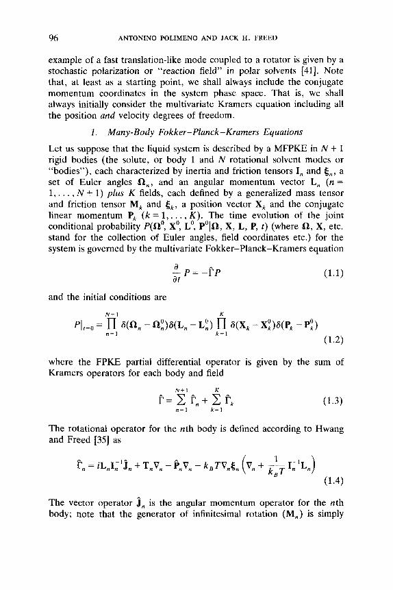
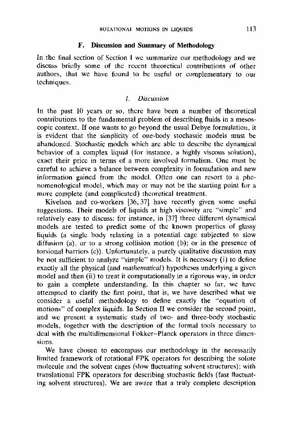
interactions, and they will be dependent only on the relative angle between u1 and u2 (see caption to Fig. 1)
-2 V 3
2 - = - V 1 P , ( Q 2 - al) - U2P2(f l , - a,) - ( plul + p2u,)X + kL3T
x2 (1.12)
here PI and P, are the Legendre polynomials of rank 1 and 2, respective- ly. Note that any direct dipole-dipole interaction between body 1 and body 2, is included in the first rank part (a minus sign has been extracted for future convenience from the first and second rank parameters).
A variety of interesting physical situations can now be obtained in the framework of the three-body model just defined, by carefully choosing the range of variation of the frictional parameters: (,, the friction exerted by the rest of the solvent on body 1, t2, the friction of body 2 and tx, the friction on the field; and the energetic parameters u l , u2, p l , p2 (2 being renormalized to 1, cf. next section). For instance, one can consider the case of a fast solute interacting via a nematic-like interaction potential with a slow (large) solvent structure in the absence or presence of a fast
Figure 1. A three-body scheme for a complex liquid. Note that uI and u2 are aligned respectively along the z , and z2 axes.
100 ANTONINO POLIMENO A N D JACK H. FREED
fluctuating field ( u , = 0, u, # 0, t2 9 6,). Or one can choose the case in which only the interaction between the solute probe and the field is present, ignoring any local structure ( u , = u2 = 0, 5, = 0). A planar Smoluchowski equivalent of this latter case was recently used for the interpretation of dielectric friction effects in polar isotropic liquids [41].
In many physical systems of experimental interest, it is usually possible to devise a reduced phase space of coordinates and/or momenta in which an accurate description is achievable. For instance, in a highly viscous fluid one may neglect all the momenta L , , L, and P given their very fast relaxation with respect the time scale relaxation of the position coordi- nates a,, a,, X. In many cases, the field vector (and its conjugate linear momentum) can be considered as a fast mode with respect to the rest of the system, so that both X and P can be projected out. One can also suppose that, although inertial effects are unimportant for the large solvent structure, that is, L2 is a fast coordinate, some inertia is still affecting the motion of body 1, so that L, must be retained. If all the additional solvent degrees of freedom are eliminated, and only a, is left, the single body Smoluchowski equation is recovered.
C. Elimination of Fast Variables
Our purpose in this section is to obtain a simpler time evolution operator from the complete one of the previous section via a systematic elimina- tion of any fast variables initially included in the system. In order to handle efficiently the algebra involved, with the smallest number of independent parameters, it is convenient to introduce from here on rescaled, dimensionless quantities (see Table I) and to “symmetrize” [42] the initial MFPK operator via the usual similarity transformation
(1.13)
where P,, is the Boltzmann distribution function over the total energy (potential plus kinetic). It is the unique eigenfunction of zero eigenvalue of the unsymmetrized operator. The final symmetrized and rescaled time evolution operator is then written explicitly
F = ui( iL,3, + T,v,) - u f e x p ( ~ : / 4 ) ~ , exp( -~ : /2 )~ , e x p ( ~ i / 4 )
+ w;(iL,Q, + T , v ~ ) - 0; e x p ( ~ ; / 4 ) ~ , exp(-~ : /2)~ , exp(~:/4)
+ uS,(PV, + FV,) - exp(P2/4)V, exp(-P2/2)V, exp(P2/4) (1.14)

ROTATIONAL MOTIONS IN LIQUIDS 101
TABLE I Rescaled Units and Parameters".h."
L l .2 = (k,TI, , ,)- l /ZL,, , F = (kBTrn)-I"P g = (k,T)-"'s"X - ( k , T ) - l / ' = - l P P l . 2 = m
w;,2 = G 6 1 . 2
w', = m-'
wi.2 = WBT) '1.2 o; = rn-1'2E
Q= ( k , T ) - I V
I .2
6x 112 - 1 ' 2
"Where the tilde symbol stands for rescaled units, and it is
bRescaled units are dimensionless except for the four w
'Subscripts 1 , 2 imply the symbol for either body 1 or
neglected throughout the text.
terms, which are in angular frequency units.
body 2.
while the rescaled potential (in k,T units according to Table I) is given by
v = - U , P , ( Q 2 - 0,) - u z P 2 ( 0 2 -0,) - ( p , u * + p2u2)X + ;x2 (1.15)
The streaming frequencies w ; and w ; in Eq. (1.14) are related to the inertial motions of body 1 and body 2, respectively (i.e., they are the inverses of the correlation times for the deterministic motion of the two bodies). The cbllisional frequencies 0; and w ; are a measure of the direct coupling with the stochastic environment, that is, of the dissipative contribution to the dynamics. An analogous interpretation may hold for the frequencies w ; and w k , related to the streaming and stochastic drift of the field.
I. Field Mode Projection
According to the previous section, we shall start by considering X and P as fast degrees of freedom, relaxing on a much more rapid timescale than the orientational coordinates and momenta of the solute and the solvent cage. Many different projection schemes are available to handle stochas- tic partial differential operators. Here we choose to adopt a slightly modified total time ordered cumulant (TTOC) expansion procedure, directly related to the well known resolvent approach. In order to make this chapter self-contained, we summarize the method in the Appendices and its application to the cases considered here and in the next section.
102 ANTONINO POLIMENO A N D JACK H . FREED
Given only that w i and wfi: are much larger than any other frequency in the system, one can easily eliminate both X and P in a simple step, via a projection based on the eigenfunctions of the monodimensional FPK operator for a single particle in a harmonic field (431. Following the detailed scheme outlined in Appendix A, after projecting out the field and its momentum, one obtains the following MFPK operator in the remaining two bodies coordinates:
F = w ; ( i ~ , 3 , + T,v,) - e x p ( ~ : / 4 ) ~ , o f e x p ( - ~ i / 2 ) ~ , exp(~: /4)
+ w i ( i ~ ~ j ~ + T,v,) - exp(~: /4)~,wS exp( -~ : /2 )~ , exp(~: /4)
- ~ x ~ ( L : / ~ ) v , w ; , exp(-~:/4 - L:/~)v, exp(~: /4)
- exp(~: /4)~ ,o ; , exp(-~:/4 - L:/~)v, exp(~:/4) (1.16)
One remaining effect from the projected fast field is given by the redefined two-body potential with respect to which the torques T, and T, are defined; the only modification is a redefined first rank potential parameter
v = -P,P1(a2 - a,) - U 2 P , ( J 1 2 -a,) (1.17)
Ul’U1 + PIP2 (1.18)
and a constant term proportional to p; + p: that we neglect since it only affects the arbitrary zero of energy.
But the major contribution of the projected fast field to the resulting operator is given by a new frictional tensor (or collisional frequency tensor), which includes coupling terms between body 1 and 2 that are of a purely “dynamic” nature; that is, they do not affect the final equilibrium distribution. The collisional matrices, modified by the averaged action of the fast field, may be expressed in the following way:
(1.19) 1 o f 1 - wlu; -(wl w 2 ) 1 / 2 u 1 u 2 “21 “ 2 - ( 0 1 w 2 ) 1 / 2 u 2 u l w;1- wzu, 2
where w1 and w2 are proportional to the field collisional frequency w‘,
(1.20)
with n = 1, 2,; U, and U2 are angular dependent 3 x 3 matrices defined as
A
U, -iJn B u n (1.21)
ROTATIONAL MOTIONS IN LIQUIDS 103
that is, the pqth Cartesian component of Uj is proportional to the result of the application of the p component of 3, on the q component of the unitary vector u,. Note that the new collisional matrix is naturally a symmetric and positive definite matrix. If it is evaluated in the molecular frame fixed on body 1 (2), the diagonal block for body 1 (2) is a constant diagonal one, while the diagonal friction block for body 2 (1) and the coupling friction blocks are only dependent upon the relative orientation
The effect of the new frictional term can be important whenever a strong initial coupling is supposed to exist between the solute and the fast mode. It is not difficult to show that a close relation exists between the frictional coupling terms of our MFPKE and the Stillman and Freed augmented Fokker-Planck equation (AFPE) in the case of a so-called “fluctuating torque” model. A close analogy between AFPE and MFPKE formalisms can be easily achieved if we consider the motion of the second body as completely diffusive. One can eliminate as a fast variable the angular momentum L, from the previous two-body MFPKE (cf. Eq. (1.16)), following again a TTOC scheme (see Appendix A). A new hybrid (partly inertial and partly diffusive) time evolution operator is found for the system (a,, a2, L , ) whose form is given as
ti? -ti1.
f = w ” , ( i ~ , Q , + T,v,) - exp(~T/4 )~ ,o ‘ , e x p ( - ~ : / 2 ) ~ , exp(~:/4)
- i exp(~ : /4 )~ , f exp( -~ : /4 - ~ / 2 ) 3 , e x p ( ~ / 2 )
- i e x p ( ~ / 2 ) j , f “ exp(-~:/4 - v / ~ ) v , exp(~:/4)
+ exp(V/2)g,D: exp(-V)Q, exp(V/2) (1.22)
with new angle dependent matrices that are defined in terms of w i , w i and oi,
(1.23)
(1.24)
(1.25)
This is a two-body AFPE that is fully equivalent to those described by Stillman and Freed, including borh a fluctuating torque effect (matrix f) and a slowly relaxing local structure (interaction potential V ) ; the equivalence of the two approaches will be further investigated in the next section for the case of a planar model.
If the momentum L, itself is considered as a fast relaxing variable, that is, the motion of the solute is supposed to be completely diffusive, then it
104 ANTONINO POLIMENO AND JACK H . FREED
is possible to further reduce the phase space to only the rotational coordinates a, and a,. The two-body Smoluchowski operator that is left after performing the I%OC projection is
f = exp(V/2)j,Dl exp(-V)j, exp(V/2) + exp(V/2)3,Dl2
x exp(-V)j, exp(V/2) + exp(V/2)j2D,,
x exp(-V)j, exp(V/2) + e~p(V/2)3~D,exp(-V)j, exp(V/2) (1.26
and we can again write down the diffusive matrix blocks in terms of of w 2 , W , ?
c c
In glassy liquids or supercooled organic fluids the viscosity affecting all the positional and orientational variables is supposed to be rather large. We can then consider a third reduced equation, describing the coupled evolution of a,, a,, X, after a straightforward elimination of all the momenta L , , L, and P from Eq. (1.14). We then easily obtain a three-body Smoluchowski equation with a 9 x 9 diffusion matrix that is diagonal and constant
F = - D, e x p ( ~ / 2 ) ~ , exp(-V)v, e x p ( ~ / 2 ) + D, exp(1//2)jI
x exp(-v) j , e x p ( ~ / 2 ) + D, e x p ( ~ / 2 ) j , exp(-v)j , e x p ( ~ / 2 ) (1.30)
and where the diffusion coefficients are related to the initial collisional frequencies, that is,
D. Planar Model
There are several reasons for considering planar equivalents of some of the above 3D-models. First of all, the heavy matrix notation employed in the previous section can be discarded, and the number of degrees of freedom for the complete system is reduced from 18 to 8 (two polar

ROTATIONAL MOTIONS IN LIQUIDS 105
angles of rotation, their conjugate momenta, which are proportional to the angular velocities, and two in-plane components for the reaction field plus their conjugate momenta). The numerical treatment of the resulting MFPK equation is easier, and a comparison between different levels of complexity in the dynamical description can be made; that is, one could consider the explicit effects of the static and the dynamic interaction between the two rotators in detail. In this way one can obtain useful insight for predicting the behavior of the much more difficult three- dimensional case. Also, one can use the planar model in order to test approximate analytical treatments.
Planar models are also important for comparing our work to some of the previous theoretical studies along the same lines, for example, the planar augmented Fokker-Planck equation described by Stillman and Freed (see next section) and the itinerant oscillator model of Coffey and Evans.
1. Planar Dipoles in a Polar Fluid
Let us consider a system made of two planar dipoles, reorienting in the xy plane of the laboratory frame, and interacting with the components XI, X 2 of a stochastic field lying in the same plane. Our starting equation, the planar equivalent of equation (1.14) is much simplified. All the frequency matrices are now scalars, the precessional terms are obviously not present and only one angular variable for each rotator has to be considered. The complete time evolution operator in a rescaled and symmetrized form is then given by
106 ANTONINO POLIMENO AND JACK H. FREED
The potential function for the system is chosen to be
v = -u1 cos(4, - 4*) - u2 cos2(4, - 42)
- ( p l cos 4, + p2 cos + 2 ) ~ 1 - ( p l sin 4, + p2 sin 4 2 ) ~ 2 + ;x: + (1.32)
We can now use our projection technique to recover averaged time evolution operators in which some of the system coordinates are consid- ered as fast. An interesting case is given by the model in which the solvent polarization relaxes faster than the reorientational molecular modes, that is, the equivalent of equation (1.16). Note that now the matrices Ul,2 (where the subscripts 1, 2 imply we are referring to both U, and U2), are simply given by (-sin cos 41,2)fr and the resulting diagonal elements of the final friction matrix are constant, so
a a aL2 dL1
- w2, exp(L:/4) - exp(- L:/4 - L:/4) __ exp(L:/4) (1.33)
and now o , , ~ and oI2 are
2 2 P l W l
* X
2 2
"x
(1.34) W1 = W f + - s2 Wf,
w2= 0; + - s2 o x (1.35) P 2 W 2 c
C L l P 2 4 4 COS(41 - 42) (1.36) w12= W21 = S 3
W X
and the potential V is again the direct interaction between the two planar rotators, with a renormalized u l . The diagonal terms of the friction
ROTATIONAL MOTIONS IN LIQUIDS 107
matrix have the well known Nee-Zwanzig form for the friction exerted by a polar viscous fluid on a reorienting dipole (dielectric friction). This is not surprising, since our model considers for simplicity only a first rank interaction between the system and its environment. Note that the frictional coupling depends explicitly only on the relative orientation (in this planar model the difference angle between the absolute angles 41 and &). as in the case of the three-dimensional model. If one neglects the frictional coupling terms, what is left is the IOM equation for two Brownian dipoles proposed by Coffey and Evans.
E. Augmented Fokker-Planck Equations and MFPKEs
The model proposed by Stillman and Freed (SF) in their 1980 paper [33] is very versatile. By choosing carefully (i) the coupling forces between molecuie variables (x,) and augmented ones (x?), and (ii) the potential function in the final equilibrium distribution, one can easily recover a variety of mathematical forms, reflecting different physical cases. The SF procedure starts from considering a system coupled to a second one in a deterministic way (interaction potential); the latter, in the absence of any coupling is described by a FP operator. The first step to obtain a description of the full system is to write the stochastic Liouville equation (SLE), according to Kubo [44] and Freed [45]
(1.37)
The Liouville operator PI contains a potential term depending on x,; the Fokker-Planck operator R , is considered for the sake of simplicity merely diffusive (so that p2 does not enter into the calculation). The SLE is not rigorous, since it does not contain terms related to the back reaction of system 1 on system 2. That is, it does not tend to the correct equilibrium, zero eigenvalue, solution. Stillman and Freed “complete” it by requiring that a given equilibrium solution Peg is recoverable. They accomplish this by modifying some reversible or irreversible drift terms, in a manner consistent with the Graham-Haken relations [46], which are based upon detailed balance, as well as with physical intuition. This finally leads to an augmented Fokker-Planck operator for the probability function. A number of points can now be highlighted. (1) The only physical aspects of the model are the interaction force f(x,, x2) in and the potential function V(xl, x2) defining P e g ; (2) the result accounts for the back reaction of 1 on 2; (3) one can usually obtain an ALE (augmented Langevin equation) from the AFPE; (4) as long as sensible choices of f and V are made, SF are able to show that the basic FP

108 ANTONINO POLIMENO AND JACK H. FREED
equation can be recovered, in the limit when x2 or p, become fast variables; ( 5 ) two main classes of models have been obtained: Puctuating torque models (only frictional effects are found), and slowly relaxing local structure models (no frictional effects, but a reorganization of the poten- tial energy is found). Finally an AFPE can be generalized to contain spin-dependent terms, treating the spin Hamiltonian as a potential. Also, other fast modes can be added in a simple way as collisional operators in the AFPE. On the other hand, some aspects of the entire procedure are not well defined. One starts with a flawed formulation (i.e., the SLE does not obey detailed balance); the next step (i.e., the modification based on detailed balance conditions) is not uniquely defined and requires physical intuition. The MFPKE while initially more constraining, leads to a more precisely defined formulation. The relation between MFPKE and AFPE is better understood in the context of the general properties of Fokker- Planck operators, that are briefly reviewed in the next section.
1. Fokker-Planck Operators: The Graham-Haken Conditions
The general operator of a FP operator is
(1.38)
where qi are a set of general variables and Kij is a symmetric tensor. Haken defines the irreversible and reversible drift coefficients as
Di = i ( K i + e iKi )
J i = 4(Ki - e,Ki)
(1.39)
(1.40)
where Tqi = Eiqi (ei = kl) , T the time reversal operator. In order that the FP has the stationary solution Peq = X exp(-V) it follows that
(1.42)
(1.43)
(note that F V = V). An alternative form of Eq. (1.38) may be obtained, in vector notation as
f = (”) J - (”) KPeq (”) Pi: as as as
(1.44)
ROTATIONAL MOTIONS IN LIQUIDS 109
In the following we shall write a general FP operator having the equilib- rium solution Peq in the form of Eq. (1.44). The vector J satisfies the following relations
.TJ= -J (1.45)
(1.46)
When J = 0 one recovers the so-called “potential condition”, which means that the operator has no reversible part.
Analysis of a Simple System According to the Stillman-Freed 2. Procedure
We consider here for simplicity a one-dimensional system constructed from a generalized solute coordinate x1 and its conjugate momentum pI coupled to a diffusive solvent coordinate x, via a potential V= Vl(xl) + V,(x,) + ynt(xl, x,). According to SF, the (renormalized and rescaled) stochastic Liouville operator is
(1.47)
The SL operator is given simply by the sum of the FPK operator for subsystem 1 plus the Smoluchowski operator for subsystem 2. It is not complete, in the sense that it does not have a meaningful solution for t+ +w, which should be the equilibrium distribution. If we require that the total system tends to the Boltzmann distribution given by the total energy (including the interaction term V,,,)
peq mexp[-(pi/2 + V, + V, + v,,,)] (1.48)
the slowly relaxing local structure model will be recovered. In this case SF modify the irreversible term in x, in a way that is equivalent to substitut- ing V, with V in the Smoluchowski part of the operator
a a - D, exp(V,/2) - exp(-V,) - exp(V,/2)
ax, ax,
a
a a
x exp(-p:/2) ~ exp( pT/4)
- D, exp(V/2) - exp(-V) - exp(V/2)
aP I
ax, ax, (1.49)

110 ANTONINO POLIMENO AND JACK H . FREED
For clarity the streaming term for subsystem 1 has been rewritten with respect to the total V; (obviously aV2/ax, = O ) . If the equilibrium is required to be independent of the interaction energy, that is,
peq = exP[-( P:/2 + VI + V2)l (1 S O )
a fluctuating torque model is obtained, with an AFP operator written as
a (1.51)
a 8x2 ax2
- D, exp(V/2) - exp(-V) - exp(V/2)
where V is now simply V, + V., and the function f is defined by
(1.52)
These are essentially SF Eqs. (4.4) (SRLS case) and (2.36) (IT case).
3. M F P K E Approach
It is easy to show that the AFPEs obtained in the previous section can be recovered from a complete system (x,, p, , x2, pz). Let us consider a FPK operator defined with the potential V(x, , x2) and the collisional matrix
(1.53)
where uin, is a general function of xl, x2, which we shall see in the following is closely related to the function f used in the SF procedure. The total MFKP operator is

111 ROTATIONAL MOTIONS IN LIQUIDS
a av a a ax, 8x2 3P2 aP2
+ ws ( p 2 - - - --) - w ; exp(p:/4) -
x exp(-p:/2) - exp(pi/4)
a a - w i exp(p:/4) - exp(-p:/2) - exp(p:/4) - wIat
a p , aP 1
a a x exp(p:/4) - exp(-p:/4 - p:/4) ~ exp(pt/4)
aP I aP2 a a
- 0 5 exp(p:/4) - exp(-p:/2) - exp(p:/4) - w,,[ 3P2 aPZ
a a X exp( p:/4) - exp(-p:/4 - pT/4) - exp( p:/4)
dPZ dP I
a dP:
(1.54)
Let us now consider the projected operator obtained when p2 is a fast variable, so that subsystem 2 is diffusive. Following the TTOC procedure, a reduced MFKP operator is recovered that is given by
ax, ax, apl
1 av 2 ax2
@ 2 dX2 8x2
- w ; [(& - - -) g s , + g q i, - - - (1.55
a a - - exp(V/2) - exp(-V) - exp(V/2)
$2 @ I
where w ; and g are given by
2 I (1.56 c @ i n , w 1 = w 1 - -
@2
@in[ g = c
@ 2 (1.57)
and the 3; are the lowering and raising operators (p1/2 T a/apl) . This reduced operator is a unified form for the cases treated by SF provided that one does not consider as an additive contribution the correction to wy. (This is due to the fact that the simple treatment of SF merely adds the collisional term in p1 as a contribution of other unspecified “fast modes” without considering in detail any dependence of the friction coefficient for the first system). For instance, if win, is chosen to be zero,
112 ANTONINO POLIMENO AND JACK H. FREED
the SRLS case is recovered; while if V is given only by V,(x,) and V,(x,) and wint is not zero, the FT case is found (just identify the SF function f with the actual g , thus relating the roles of V,,, in the SF approach and win, in the MFPK model through Eqs. (1.52) and (1.57)). From a purely algebraic point of view it is straightforward to understand why the AFPEs recovered by SF are so intimately related to a bidimensional MFPKE. In fact, it is clear that SF can obtain a model that is consistent with simple MFPKE provided that they modify, according to Haken’s conditions, only the irreversible drift coefficients (vector D) and the reversible drift coefficients (vector J) without changing the assumed diffusion tensor (matrix K). The initial system in the SF derivation is made by a Kramers subsystem (xl, pl) and by a diffusive one x2
Pe,=.N”exp(-~p,-Vl-V,) 2 (1.58)
(1.59)
(1.60)
Here J , is associated with x , , J2 with p l , J3 with x2. The SL approach requires that we modify J by adding a term to the partial derivative of V,,, with respect to x i
(1.61)
This is the reactive force on the first system as a result of its interaction with the second system. In order to obtain a proper equation in the SRLS case, SF modify the irreversible term in x 2 , that is, D,. In the present notation this is merely equivalent to substituting Eq. (1.59) by Eq. (1.48). In the FT case SF modify J 3 ; that is, they add a term -wsp,fto the reversible drift coefficient in x 2 , which was previously zero, and leave P,, unmodified. In both cases these are the minimal modifications required to achieve detailed balance. No changes in the diffusion tensor elements are introduced, although such possibilities exist. This “minimum effort” choice yields equations derivable from a MFPKE in which the full set of variable ( x i , p, , x 2 , p 2 ) is considered.
ROTATIONAL MOTIONS IN LIQUIDS 113
F. Discussion and Summary of Methodology
In the final section of Section I we summarize our methodology and we discuss briefly some of the recent theoretical contributions of other authors, that we have found to be useful or complementary to our techniques.
1 . Discussion
In the past 10 years or so, there have been a number of theoretical contributions to the fundamental problem of describing fluids in a mesos- copic context. If one wants to go beyond the usual Debye formulation, it is evident that the simplicity of one-body stochastic models must be abandoned. Stochastic models which are able to describe the dynamical behavior of a complex liquid (for instance, a highly viscous solution), exact their price in terms of a more involved formalism. One must be careful to achieve a balance between complexity in formulation and new information gained from the model. Often one can resort to a phe- nomenological model, which may or may not be the starting point for a more complete (and complicated) theoretical treatment.
Kivelson and co-workers [36,37] have recently given some useful suggestions. Their models of liquids at high viscosity are “simple” and relatively easy to discuss: for instance, in [37] three different dynamical models are tested to predict some of the known properties of glassy liquids (a single body relaxing in a potential cage subjected to slow diffusion (a), or to a strong collision motion (b); or in the presence of torsional barriers (c)). Unfortunately, a purely qualitative discussion may be not sufficient to analyze “simple” models. It is necessary (i) to define exactly all the physical (and mathematical) hypotheses underlying a given model and then (ii) to treat it computationally in a rigorous way, in order to gain a complete understanding. In this chapter so far, we have attempted to clarify the first point, that is, we have described what we consider a useful methodology to define exactly the “equation of motions” of complex liquids. In Section I1 we consider the second point, and we present a systematic study of two- and three-body stochastic models, together with the description of the formal tools necessary to deal with the multidimensional Fokker-Planck operators in three dimen- sions.
We have chosen to encompass our methodology in the necessarily limited framework of rotational FPK operators for describing the solute molecule and the solvent cages (slow fluctuating solvent structures); with translational FPK operators for describing stochastic fields (fast fluctuat- ing solvent structures). We are aware that a truly complete description
114 ANTONINO POLIMENO AND JACK H . FREED
should also include in a many-body stochastic view, the interaction between the rotational and translational degrees of freedom of the solute and/or of the solvent. In addition, one can use different formal ap- proaches to obtain improved (i.e., many-body) kinetic equations for the orientational distribution of a solute molecule strongly interacting with the solvent. In this respect, Bagchi et al. [47] have recently provided an analysis for explaining the anomalous rotational behavior of glassy liquids by including the translational motions of the solvent molecules and the density fluctuations of the solvent in the Debye-Smoluchowski descrip- tion, which is particularly interesting since it could provide links between mesoscopic stochastic theories and advanced microscopic and mode-mode coupling treatments. They obtain an integro-differential kinetic equation in the orientational distribution probability function of the solute, which is appropriate for highly viscous fluids only. No explicit mean field potential or inertial effects are included.
Finally rototranslational coupling has been investigated in two recent papers by Wey and Patey [48,49], using the general approach of the Van Hove functions described within the Kerr approximation, which relates the rototranslational correlation function of the solute to the joint conditional probability in both the position and orientation of the mole- cule. This method is helpful in providing a physical and mathematical framework for rototranslational coupling in complex fluids. However, it requires as a starting point a well defined equation of motion for the conditional probability. Wey and Patey have tested only one-body sto- chastic equations (such as the Fick-Debye and the Berne-Pecora equa- tions), which are necessarily restricted.
2. Summary
We have attempted to provide a general approach to build multi- dimensional stochastic operators of the Fokker-Planck-Kramers type, for describing the time evolution of an extended set of degrees of freedom in complex liquids. This set contains the orientation of a probe molecule (first body) and its conjugate angular momentum vector, plus similar coordinates for a collection of N bodies. Each of them is an additional solvent body. Also, a collection of K stochastic fields is introduced. The time evolution operator for the system of 6 X ( N + K + 1) degrees of freedom is given by a sum over rotational and translational FPK operators. The only source of coupling (at this stage) is given by a potential depending on the mutual orientations of each body and field.
For the case of two rotators and one stochastic field (N = 1 and K = l), it has been shown (using a TTOC expansion procedure) how to eliminate, as fast variables, some of the original degrees of freedom (e.g., the
ROTATIONAL MOTIONS IN LIQUIDS 115
stochastic field and its momentum) in order to obtain models which contain coupling terms just in the friction tensor of the rotators. The reduced two-body Fokker-Planck-Kramers (2BFPK) equation has been shown to be formally equivalent to the augmented Fokker-Planck equa- tion described by Stillman and Freed [33]. In the planar case, that is, when both the probe and the solvent body are described as planar dipoles, and any residual frictional effect due to a fast field is neglected, one obtains the IOM equation of Coffey and Evans [23-251.
11. COMPUTATIONAL TREATMENT
A. Introduction
In the first section we have discussed a general methodology for the theoretical description of rotational dynamics of rigid solute molecules in complex solvents. Many-body Fokker-Planck-Kramers equations (MFPKE), including collective solvent degrees of freedom (either rota- tional ones, i.e., rigid bodies, or translational ones, i.e., vector fields), and their conjugate momenta, have been described as convenient tools to reproduce (or simulate) the complexity of an actual liquid system.
In Section 11, we apply our stochastic models to physical systems of interest. Although the methodology was developed mainly to interpret complex features of ESR spectra over a wide range of temperatures, viscosities and solvent compositions, we believe that it could profitably be applied to many other experimental techniques, sensitive to rotational dynamics effects (such as dielectric relaxation, Raman and neutron scattering, NMR measurements) in liquids. Preliminary results on two- and three-body models, have been encouraging for the study of “slowly relaxing local structure” (SRLS) and “fluctuating torque” (FT) effects in isotropic liquids at moderate and high viscosities [39]; and for the interpretation of the bifurcation phenomenon in glassy and supercooled fluids [40]. Here we describe in detail the computational approach that is needed to treat many-body MFPK operators, provide extensive results on several rotational models, and discuss their application for interpreting liquid behavior.
In Section 1I.B we briefly review the usage of the complex symmetric Lanczos algorithm for treating MFPK operators, with particular attention to the problem of the choice of a suitable set of basis functions for a many-body problem. In Section 1I.C we consider the case of two spheri- cal rotators in a highly damped fluid (Smoluchowski regime) as a first example of the application of angular momentum coupling techniques to Fokker-Planck operators (two-body Smoluchowski model, 2BSM). This
116 ANTONINO POLIMENO AND JACK H. FREED
approach is extended in Section 1I.D for studying a three-body system (two rotators plus one field), again in the overdamped regime (3BSM). Sections 1I.E. and 1I.F are devoted to the analysis of two-body models in the full phase space of rotational coordinates and momenta of the two rotators (two-body Kramers models, 2BKM), for a total of twelve degrees of freedom, all fully coupled together, at least in principle. Section 1I.G. contains a discussion of results concerning the various models, Rotational correlation functions and momentum correlation functions for body 1 are discussed, together with their dominant eigen- values; a detailed analysis of the dominant eigenmodes of the system is given in each case.
Finally, a comparison of the MFPKE approach with molecular dynamics, ESR and stimulated light scattering experiments is contained in Section 1I.H. Detailed formulations of reduced matrix elements are given in Appendix C.
B. Computational Strategy
A powerful and general method for numerical solution of Fokker-Planck (FP) operators has been given by Moro and Freed [50]. It involves first establishing a complex symmetric matrix representation with a basis set of orthonormal functions, followed by a tridiagonalization procedure utiliz- ing the Lanczos algorithm. The usage of the conjugate gradient algorithm as an alternative procedure to tridiagonalize the initial matrix has been considered by Vasavada et al. [Sl]. A thorough review of the usage of iterative algorithms for solving stochastic Liouville and FP equations has been provided by Schneider and Freed [42]. The interested reader can consult this reference for further details. In this section we will focus our attention on the optimization, for the many-body systems considered, of the matrix representation rather than on the detailed computational treatment of the matrix itself.
We start with the time-dependent conditional probability for the stochastic system P(q"lq, t ) , where q is a complete set of stochastic variables. The time evolution of P is governed by the Fokker-Planck- Kramers (FPK) equation [cf. Eq. (1.1)]:
with the intial condition [cf. Eq. (1.2)]
In the following, q will be the collection of rotational coordinates a,,
ROTATIONAL MOTIONS IN LIQUIDS 117
In,, . . . , I n N + , and fields X I , X , , . . . , X , and of their conjugate momenta L, , L,, . . . , LNcl and PI, P2, . . . , PK (cf. Section I .B. l ) . The operator f is given as a sum of FPK operators, each of them defined in the (a,,, L,) or (Xk,Pk) subspace. The total energy E of the system is given by the potential energy of interaction plus the total kinetic energy, and it defines the equilibrium distribution Peq(q), that is, the unique eigenfunction of f with a zero eigenvalue. Thus
2 n = l k = l (2.3)
where ( ) standard for the integration on the full phase-space of q coordinates and momenta. It is useful to apply a similarity transformation to f , which renders it possible to obtain a complex symmetric matrix representation of the operator (or a real symmetric one, if f is Hermi- tean). The transformation is simply [cf. Eq. (1.13)]
(2.5) f = p - l / ’ f p l / ’
eq eq
note that the “symmetrized” operator has the same eigenvalues as the unsymmetrized one, yhile the eigenfunctions are multiplied by Pi:”. Then by representing r in a complete orthonormal set of basis functions that are invariant under the classical time reversal operation, a complex symmetric matrix representation is guaranteed [42].
1. Correlation Functions, Spectral Densities and Lanczos Algorithm
Usually we are interested in the (auto)correlation function G(t) of an observable (i.e., a function of some stochastic coordinates). In the following we will consider either rotational correlation functions (i.e., involving the spherical harmonics y.m(Inl )) or momentum correlation functions (i.e., involving the components of L , ) for the first rotator (body l ) , identified as the solute molecule
118 ANTONINO POLIMENO AND JACK H . FREED
Following the procedure developed by Moro and Freed, one obtains a matrix representation of f and a vector representation of the function FPLf (where F is the observable, for example, Y,m(f l l ) or Ll,) , utilizing an appropriate set of basis functions. Given the (complex) symmetric matrix r and the "right vector" v (formed from F P L f ) , one is left with the evaluation of the resolvent, the generic form of which is
J ( & ) = v . (iwi + r)-l (2.10)
We shall set N be the dimension of the finite basis subset used to represent f and v. The calculation can be performed with great efficiency using an iterative algorithm, such as the Lanczos algorithm, that trans- forms r into a tridiagonalized form. A continued fraction expansion is then obtained:
2 2 P n - 2 P n - 1 PZ P : . . . J ( N , " y w ) = 1
iw + al- io + a2- iw + a3- iw + a,-l- iw + a, (2.11)
where n is the number of iterations (Lanczos steps) necessary to achieve convergence; usually n 4 N. The ayi coefficients are the diagonal elements of the tridiagonal complex symmetric matrix, whereas the Pi are the extradiagonal ones. Given the tridiagonal matrix, one can also calculate the eigenvalues Ai associated with the spectral density, by means of an efficient diagonalization procedure for tridiagonal matrices (e.g., the QR algorithm).
In practice, although the entire procedure has been shown to be extremely effective in dealing with stochastic systems of 2-3 degrees of freedom (as well as in a stochastic Liouville equation with spin coordi- nates as well), its application to larger systems (with degrees of freedom ranging from 4 to as many as 12) is not so straightforward, because of a
ROTATIONAL MOTIONS IN LIQUIDS 119
dramatic increase in computation time and memory space requirements, even if a powerful supercomputer is used. The bottleneck is usually the matrix dimension N , which can be very large. It is therefore of consider- able importance to optimize the basis set utilized to represent the operator in order to minimize N .
C. Two-Body Smoluchowski Model
The model that we are going to consider in this section is given by two spherical rotators, simply called body 1 and body 2. Body 1 is the solute molecule, whereas body 2 is the instantaneous structure of solvent molecules in the immediate surroundings of the solute. The rest of the solvent is described as a homogeneous, isotropic and continuous viscous fluid. In the overdamped regime, the system is described by a Smoluchowski equation in the phase space (a,, a,), where In, and a2 are respectively the set of Euler angles specifying the orientation of a fixed frame on body 1 with respect the lab frame, and an analogous set for the orientation of a fixed frame on body 2.
In accordance with Table I , we will adopt from the beginning a dimensionless set of units. The symmetrized, rescaled time evolution operator for the model is then (compare with equation (1.30) for the three-body case)
(2.12)
The equilibrium distribution function P,, is defined according to Eq. (2.4); but the relevant part of the total energy is given just by the (rescaled to k , T ) potential energy function V (cf. Section I)
V(f i , , st?) = -c U R P R ( f i 2 - f i l l (2.13)
where PR(f i ) is the Legendre polynomial of rank R , and Eq. (2.13) implies that U depends only on the relative orientations of bodies 1 and 2 (the minus sign is only for convenience). We shall consider the expansion of Eq. (2.13) up to R = 2 (Le., only first or second rank interactions are included). 3, and 3, are respectively the “angular momentum” operators for body 1 and for body 2 in the laboratory frame of reference. For future usage, we define also the total “angular momentum” operator of the system as
R
j=j , + Q 2 (2.14)
and we rewrite f in a more convenient form for the actual calculation of
120 ANTONINO POLIMENO AND JACK H . FREED
the matrix elements (although less elegant than Eq. (2.12)) as
= D,j : + D,j: + D,G, + D,G, (2.15)
where the functions G , (m = 1 , 2 ) are defined
1 1
4 G m = - ~ : z + 5 ( j rnTrn) fun (2.16)
and where ( )fun indicates that what is contained within, acts as a function, not an operator. Also, T, is the torque acting on body m due to V, that is,
A
T,, = -iJ,V (2.17)
1. Uncoupled and Coupled Basis Sets
A simple choice for a complete basis set of functions for obtaining a matrix representation r is the uncoupled set
where each function IJ,M,K,) is given by [53,54]
(2.19)
Hereafter we let [ J ] = 25 + 1. This is a complete orthonormal set given by the direct product of Wigner functions in the set of Euler angles a , and a,. Note that since the phase space is six dimensional, we have six distinct quantum numbers to cope with. However, the potential V that we have chosen is independent of the azimuthal angles y, and y2, and this is reflected in the fact that r will be diagonal in K , and K,. In the following, the K,, quantum numbers will be discarded from any formula, if not otherwise specified, since only the matrix block with K , = K2 = 0 will be of interest.
It is possible to further reduce the number of effective (nondiagonal) quantum numbers taking advantage of the spherical symmetry of the fluid to determine other “constants of the motion” (note however that a11 the following considerations also hold for molecules with cylindrical symmet- ry). Let us consider the tensorial properties of the functions and operators defined in the previous paragraph with respect the “total”
ROTATIONAL MOTIONS IN LIQUIDS 121
angular momentum operator 3 given by Eq. (2.14). Obviously, 3, and 3, are themselves first rank tensor (i.e., vector) operators. Furthermore, one may rewrite the Rth component of the potential
R
u R P R ( s ~ , , ~ ~ ) = - v R C (-)’IR-SO),IRSO), (2.20) S = - R
in a form clearly showing its nature as a zero rank tensor (scalar) with respect to 3. Note that
V d R l U R = -
8rr2 (2.21)
Since it is simply an exponential funstion of V , Peq is also a scalar. It follows directly from Eq. (2.12) that r itself is a scalar, as it must be to satisfy Eq. (2.1). One can also arrive at this result from Eq. (2.15), noting that T, and T2 are vector operators. It is also easy to see that
The vector T will simply be called the “torque” in the following, without specifying any index. Note also that G, = G, = G.
From these considerations, one concludes that the coupled basis set
where C(J ,M,J ,M, J M ) is a Clebsch-Gordan coefficient, is the most suitable set of basis functions for the present problem ( K , and K , have been neglected). In fact, due to spherical symmetry, both J and M are “good” quantum numbers, that is, r is diagonal in them (note that this is still true for cylindrical spatial symmetry, while for the completely asymmetric case only J is a “good” quantum number).
The initial vector v must also be evaluated. Instead of computing directly the vector representation of the given rotational function (i.e., the spherical harmonic in a,, which is an element of the uncoupled basis set), one can evaluate the matrix representation of the function, which we call M, and then multiply it by the vector representation of P::, which we call vo, whose calculation is relatively easy utilizing the coupled basis set (see Appendix C.2). That is, let
v = Mv, (2.24)
122
Then
ANTONINO POLIMENO AND JACK H . FREED
where A stands for the collection of quantum numbers, and the rotational observable F is simply the basis vector IPQO), that is, the Qth compo- nent of the P rank rotational function in ill. One can see by inspection that only the elements with J = 0, M = 0 are not zero in the vector vo, and that only the matrix block defined by the conditions J ' = O , M ' = O , A(JPJ') , M = Q has to be considered in M (A is the triangle condition); then the only nonzero elements of v are those for which J = P, M = Q. It follows that the only matrix block we need to compute in r satisfies the conditions J = P, M = Q.
2. Matrix Elements A clear advantage of employing angular momentum coupling techniques is the possibility of using the Wigner-Eckart (WE) theorem to simplify the calculation of matrix elements in the coupled basis set [4]. In this two-body case, only two nondiagonal quantum numbers, J , and J2 have to be considered. (In general, if N + 1 rotators are present, a generalized coupled basis set allows one to have 2 N effective nondiagonal quantum numbers.)
Let us now consider f given by Eq. (2.12). The terms proportional to and j i are diagonal; and we may write for the matrix element of Eq.
(2.12)
where the sets A and A' are characterized by K , = K ; = 0, K 2 = K ; = 0, J = J' = P, M = M' = Q. The matrix element of G is
that is, it is reduced to a sum of matrix elements of scalar products of operators of form A - B . (For future convenience, we will call r,, the complete matrix element without the factor C ~ ~ ~ . S , , . .)
ROTATIONAL MOTIONS IN LIQUIDS 123
In general one finds, from the WE theorem (weak form for noncom- muting operators)
x ( J ; .I; J” I I B I I J ; J ; J’)6,, 3 6,, t (2.30)
where 8, B are either f l or T. The reduced matrix element o f f , is given by (see [41)
J,+J2+J’+1[JJ,l l /2 [ J’, J J 2 ) ( J l J 2 J I l ~ l I I J I J ; J ’ > = (-1 J J , 1
and the reduced matrix element of T is evaluated in Appendix C.l. The final matrix r is real symmetric. (Note that [JJ‘] = [J][J’]).
The matrix element (M)AA. of Eq. (2.27) is easily computed from the WE theorem, and one obtains
with J = P, M = Q , J’ = 0, M‘ = 0 and K , = Kj = K2 = K ; = 0. No ex- plicit dependence on Q is present; that is, given the spherical symmetry, all the rotational correlation functions are independent of Q. The compo- nents of the vector v,, are calculated in Appendix C.2.
D. Three-Body Smoluchowski Model
A further elaboration in describing the rotational dynamics of a solute in a complex environment is obtained by increasing the number of interact- ing solvent modes included in the time evolution operator. Theoretically, one could consider a new set of collective degrees of freedom for each relaxation process that is relevant for the solute dynamics. In practice, computational problems soon arise. However, a three-body description can still be treated rather easily, and it is the subject of the present section. Instead of considering a third rotational set of coordinates, we have chosen to define the third “body” as a stochastic, vector-like field X. One can think of a polarization coordinate, or of the fluctuating solvent dipole moment interacting with the probe. We shall consider only first rank interaction between the solute body and the solvent structure with the stochastic field. The effect of a fast field, as a source of a “fluctuating
124 ANTONINO POLIMENO AND JACK H . FREED
torque” relaxation mechanism on the solute dynamics has already been partially explored. A summary of our computational results is presented in a later section. Here we deal with the formulation of the three-body model and its detailed mathematical treatment.
1 . The Model
The symmetrized and rescaled time evolution operator for the system described by the set (In,, In,, X) is simply defined adding to the two-body operator in Eq. (2.12) the translational Smoluchowski term for the field to obtain [cf. Eq. (1.30)]
where V, is the gradient operator in the X subspace. The equilibrium distribution function is now defined with respect the following potential
Note that the dimensionless units defined in Table I are used, so that the curvature along the X direction is renormalized to 1. Here U, is the two-body interaction potential defined in Eq. (2.13). The two terms linear in X are the “dipolar” interaction energy (with u, and u, two unit vectors, respectively, along the z-axis of the fixed frame for the solute and the solvent body, cf. Fig. 1). Finally a quadratic term in X has been added in order to confine the fluctuations of the stochastic field.
2. Matrix Representation
An efficient treatment of the time evolution operator defined in Eq. (2.33) can be achieved by performing a canonical transformation of coordinates acting on the field X. We define the shifted vector X-.X - plu, - p,u, as a new set of field coordinates. The potential is now decoupled
V(In,, In,, X) = V,(In,, In,) + ;x2 (2.35)
Note, however that the first rank coefficient in V, is modified slightly as u1 j. u 1 + pl p,. Although the potential form is simplified, new terms arise in the operator itself. Skipping straightforward algebraic details, the following equation is obtained:
ROTATIONAL MOTIONS IN LIQUIDS 125
f = f, + D,$+S-
- D , ~ ~ ( ; T , + i j I ) ~ , S - + D , ~ , S + U ~ ( ~ T , - i j , )
- D 2 k ( i T 2 + &)U2S- + D,p2S+U2( $T2 - is,) - DIp:S+UtS- - D2pii$+UiS- (2.36)
where S* = 4X 7 V, are the lowering and raising (vector) operators for the three-dimensional harmonic oscillator X. T, and T, are the torques for body 1 and 2, respectively, due to V, (TI = -T, = T); finally U , and U, are 3 X 3 matrices defined (for m = 1,2) as
U m = i ( j m 8 Urnl fun (2.37)
F0 is the two-body Smoluchowski operator given by Eq. (2.12). We now have to treat a system of 9 degrees of freedom. It is possible
to use techniques of angular momentum coupling that are analogous to those employed for the two-body case. We define the angular momentum operators
j= -ixxV, (2.38)
j , = j + J (2.39)
and j is defined according to Eq. (2.14). In the following we will sometimes call 3 ‘‘little’’ angular momentum, 3 “big” angular momentum and 3, “total” angular momentum. We use a double coupling scheme to determine the most convenient basis set for the problem. We start from the uncoupled basis set
I J , M , K , ; J ,M,K, ; m> = IJ,M,K,)IJ,M,K,)Injm) (2.40)
given by the direct product of the uncoupled two-body set with the functions Injm) defined in terms of the polar coordinates X , 6 and q5 for the field; that is,

126 ANTONINO POLIMENO AND JACK H . FREED
where 2: is the pth order Laguerre polynomial of degree q [52]. As in the previous case, two quantum numbers, K , and K,, are obviously diagonal. Note that the system is still spherically symmetric and the potential does not depend on the Euler angles y, and y,. We shall neglect K , and K, in the following whenever possible, since only the matrix blocks with K , = K , = 0 will be computed.
We may proceed in our coupling scheme by first considering the coupling of f , and f , to give f ,
(J ,J ,JM; njm) = c C ( J , M , J , M , J M ) I J , M , ; J2M2; njm) (2.44)
In this basis set only the two-body operator F, is diagonal with respect to J and M . A fully coupled basis set is then obtained by coupling together 3 and f to give 3,
InJ,J,JjJ,M,) = C(JMjmJ,M,)IJ,J,JM; njm) (2.45)
J , and M , are “good” (i.e., diagonal) quantum numbers for f . Note that from an initial nine-dimensional problem, we are left with a five-dimen- sional one. The relevant quantum numbers are n , J , , J , , J and j .
The calculation of the matrices r and M, and the vector vo can now proceed along the same lines as the previous section. The general vector element ( v , , ) ~ is exactly the same one given by Eq. (C.10) in Appendix C.2, but the factor 9 in that equation is now 6JTo6MT,6n,6,06,0. The matrix element (M)A,At is simply
MlM2
rnM
(A[FlA’) = 6 J 2 J 2 !6 J 1 J 2 .6 J P 6 I 0 I 6 nn Jii! (8 IT’)’ (2.46)
with J , = P, M , = Q , J k = 0 , M k = O . It follows that the only matrix block of that is needed is defined by J , = J k = P and M , = M k = Q. The matrix r is obtained by a systematic usage of the WE theorem. We may write F of Eq. (2.36) in the straightforward but convenient form
+ D1pl(O; + 0,) + O2p2(0): + 0,)
+ Dip;$ : c, + D,&S : c2 (2.47)
where the double dot symbol means the scalar product of two second rank Cartesian tensors. Here r, is the two-body operator; 0, and 0, are
ROTATIONAL MOTIONS IN LIQUIDS 127
vector operators, while 6, G I and Gz are matrix operators, introduced for their convenient tensor properties (cf. below). They are defined according to the following equations (rn = 1,2):
(2.48)
s = $ + $ - I r (2.49)
(2.50)
O , = S - + U , , , X ( ~ T , - ~ ~ , )
G m =-u2 m 3 - 2 1
where we have systematically used a Cartesian notation for representing the various tensor products and the general property of the matrix U, is given in terms of the unit matrices u,, by
Ulnr = u, X r (2.51)
where r is a generic vector. We can now consider each term separately. The two-body operator Fo
has the same matrix representation in the two-body coupled basis set and in the present three-body coupled basis set. The next term in S S is diagonal in the chosen basis set [4]. Then the matrix representation of these diagonal terms is
,.+A’-
The term with off-diagonal elements from Ol is considered next. From the WE theorem (strong form), and using the equivalence between a first rank tensor product and the external product of two vectors, we obtain
I + j + J ’ + J , J i J (A10;lA’) = i(2)’”(-) (i‘ J , T ]
x ( J , J~J (~ [U, CQ( ; T ~ - i ~ l ) ] ( l ) l l ~ ~ ~ ; ~ ’ )
x (ni I I s + I I n ‘i ) aJrJ + aMTM (2.53)
The reduced matrix element of ,$+ is evaluated in Appendix C.3; the reduced matrix element involving ul is straightforwardly evaluated using the general formula
( J + I + J ’ ) 2 { I 1 I } J J” J ’ (J,J,JII[;i €3 B]‘”(IJ;J;J’) = [1]”’(-)
J ; I ; I”
128 ANTONINO POLIMENO AND JACK H . FREED
where and B can be T , , j,, u , . The reduced matrix element of the torque and of the angular momentum operator are given respectively in Appendix C. 1 and in the previous section. The reduced matrix element of u1 is proportional to the reduced matrix element of the function 1100), (see Appendix C.l)
(Jlll1llJI) [1]1/2 (8 n-2)1'2
X (2.55)
where (Jl(I111J;) is the reduced matrix element of a first rank spherical harmonic. The matrix element proportional to 0: is obtained by exchang- ing A and A' in the previous formulas. The matrix elements of 0, and 0; are evaluated in a similar manner.
Finally the matrix elements of the mixed operators in GI and G 2 may be considered. Both 5 and el (G , ) are second rank spherical tensors. It follows that
and the reduced matrix element of !$ is given in Appendix C.3. The reduced matrix element of GI is proportional to the reduced matrix element of the function 1200),
The calculation of the matrix element of g : G , proceeds along the same lines. Note that, as was the case with the two-body problem, a real symmetric matrix is obtained.
E. Two-Body Kramers Model: Slowly Relaxing Local Structure
The next model considered in this work is Kramers description of a two-body system, that is, the generalization of model (a) in order to account for inertial effects. The time evolution operator is given by a
ROTATIONAL MOTIONS IN LIQUIDS 129
Fokker-Planck-Kramers rotational operator involving the rotational coordinates of bodies 1 and 2, and their conjugate angular momenta, L, and L,. The final phase space to be considered is then twelve-dimension- al. In practice, we will find that only eight effective (nondiagonal) quantum numbers need to be considered in a properly chosen coupled basis set of functions, for two spherical (or symmetric) rotators. Still, the matrices needed for computations have huge dimensions, and the numeri- cal treatment is far from easy, especially when large potential couplings and/or low friction regimes are explored.
1 . Slowly Relaxing Local Structure Model
Again we consider the symmetrized and rescaled time evolution operator, obtained by summation of the two rotational FPK operators €or bodies 1 and 2, in the presence of the usual interaction potential. Since we suppose that both the bodies are spherical, no precessional terms are present [6] [cf. Eq. (1.14) €or the three-body case]:
The same definition and properties of the torque vectors holds as in Eq. (2.17); V, and V2 are the gradient operators acting respectively in the subspaces L, and L,. The frequency parameter w ; is the streaming frequency; it is the characteristic frequency for the deterministic motion of body 1 and it is inversely proportional to the square root of the moment of inertia I,. wf is the collisional frequency of body 1, and it is a direct measure of the dissipative effect due to the solvent, since it is proportional to the friction exerted by the medium on the body. Analog- ous parameters 6-1; and w i are defined for body 2. See Table I for the explicit definitions.
The equilibrium distribution function is defined with respect to the total energy of the system
E = v”(n,, a,) + tL; + :L; (2.59)
including the interaction potential between the two bodies and the (rescaled) kinetic energy. The coupling between body 1 and body 2 is given only by the potential; no “hydrodynamic” interactions, that is, frictional coupling terms, are included. A situation close to models in which the solute (body 1) reorients in a potential resulting from a slowly

130 ANTONINO POLIMENO AND JACK H. FREED
relaxing solvent local structure (body 2) is then recovered, as was discussed previously.
2. Matrix representation
The numerical treatment is again based on the matrix representation of the operator on a coupled basis set of functions, followed by the application of the Lanczos algorithm. Following the same method used in the previous section, we define the two ‘‘little’’ angular momentum operators (one for each body) and the overall “little” angular momentum operator
3, = -iL, x v, (2.60)
3, = -iL, x V, (2.61)
j=j, +j2 (2.62)
and the total angular momentum operator . . A
j , = j + J (2.63)
where 3 is defined by Eq. (2.14). It is easy to see that f is a scalar with respect to 3,. The initial uncoupled basis set is given by
lJ,M,K,; J,M2K2; n l j lm, ; n,i,m,>
= lJ,M,K, )IJ2M2&) x l ~ 1 ~ 1 ~ , ~ l ~ 2 ~ 2 ~ 2 ~ (2.64)
where the functions In,j,m,) and In,j,m,) are defined with respect to the polar coordinates L , , O , , 6, and L,, O,, y2, respectively. As usual, the K , and K , quantum numbers are diagonal and will be neglected in the following. The coupling scheme involves the coupling of 3, and 3,; then the coupling of j, and j,; finally 3 and are coupled together to give j T .
) J I M , ; J2M2; n ,n2i , i , j4
= c C(j,m,j2m,jm)IJ,M,; JzM,; n , j ,m, ; n,j,m,> m1m2
(2.65)

ROTATIONAL MOTIONS IN LIQUIDS 131
The total angular momentum quantum numbers, J , and M , are diagonal, that is, “constants of motion”.
The calculation of the matrix r is now a straightforward application of previous formulas. The vector representation of P again has the ele- ments defined in Appendix C.3, where 9 IS now equal to 6JToSM70Sj06j10Sj20Snl~6n~o. The matrix elements for the rotational correla- tion function ( F = Y p a ) (MR)A,A, are given by
e9
and J , = P, J ; = 0, M , = Q , M k = 0, K , = KI = K , = K ; = 0; whereas the matrix elements (MJ)A,A, for the momentum correlation function (mth spherical component of the first rank tensor L , , F = L, ) are given by
I (AIFln,) = ( - ) l + / , + l ~ + J [ l J ] - ~ ~ ? [ j , f ] l i 2 (ii ;, 1 2
1 1
x ( a ,il IIL, I 1 4L )6JlJi aJ2Ji 6 J J ” J j ’ 6 n 2 n ~ 6 j 2 j ~ (2 .69)
and J , = 1, J ; = 0, M , = m, M ; = 0, K , = KI = K, = K ; = 0. We con- clude this section by writing down the complete matrix element for the time evolution operator:
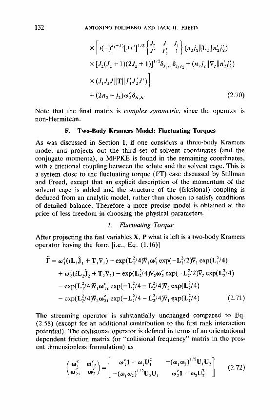
132 ANTONINO POLIMENO AND JACK H. FREED
(2.70)
Note that the final matrix is complex symmetric, since the operator is non-Hermitean.
F. Two-Body Kramers Model: Fluctuating Torques
As was discussed in Section I , if one considers a three-body Kramers model and projects out the third set of solvent coordinates (and the conjugate momenta), a MFPKE is found in the remaining coordinates, with a frictional coupling between the solute and the solvent cage. This is a system close to the fluctuating torque (FT) case discussed by Stillman and Freed, except that an explicit description of the momentum of the solvent cage is added and the structure of the (frictional) coupling is deduced from an analytic model, rather than chosen to satisfy conditions of detailed balance. Therefore a more precise model is obtained at the price of less freedom in choosing the physical parameters.
1. Fluctuating Torque
After projecting the fast variables X, P what is left is a two-body Kramers operator having the form [i.e., Eq. (1.16)]
The streaming operator is substantially unchanged compared to Eq. (2.58) (except for an additional contribution to the first rank interaction potential). The collisional operator is defined in terms of an orientational dependent friction matrix (or “collisional frequency” matrix in the pres- ent dimensionless formulation) as
(2.72) 1 W f l - WJJ; - (w ,W2) ’ /2u ,u , - ( W 1 W 2 ) 1 / z u 2 u 1 w;1- W 2 U 2 2

ROTATIONAL MOTIONS IN LIQU1,DS 133
where are defined with respect p1,2, D, [see Eqs. (1.19)-(1.21)]. Obviously, all the new collisional terms retain the characteristic tensorial properties allowing the use of the same coupled basis set as in the previous section.
2. Matrix Elements
The calculation of the matrix M and the starting vector v proceeds exactly along the same lines discussed in the previous paragraph (since they depend only on the structure of P,,). The matrix element r can be conveniently evaluated by Eq. (2.71) in the form
+ [ S y l + S y ] : [ ( w ; + 502) l+02eI] 2
where
(2.74)
g y = gl+ 0s; - S1(0)1 (2.75)
gg) = 6: . g ; (2.76)
9;;) = $+ 8 8 ; - qq (2.77)
with i, j = 1 , 2 ( i # j ) . These are the zero and second rank irreducible tensors built from Slz, the raising and lowering operators in L,
1 . sl- ^ ( O ) - - g +
Sl - 3 I
3
g z 1 = 1 2 Ll Ql (2.78)
The collisional operator is obtained by taking the product with the zero and second rank irreducible tensors built from U,,-that is,
(2.79)
(2.80)
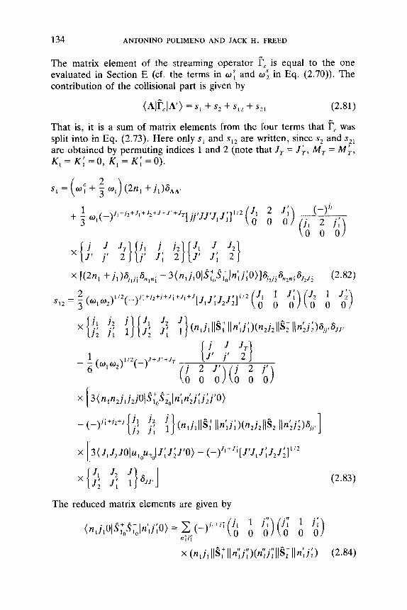
134 ANTONINO POLIMENO AND JACK H. FREED
The matrix element of the streaming operator f5 is equal to the one evaluated in Section E (cf. the terms in uf and w i in Eq. (2.70)). The contribution of the collisional part is given by
{ hlFcJh’) = s, + s2 + s I 2 + s2, (2.81)
That is, it is a sum of matrix elements from the four terms that Fc was split into in Eq. (2.73). Here only s, and s , ~ are written, since s2 and s21 are obtained by permuting indices 1 and 2 (note that J , = J k , M , = Mk, K = K ’ = O K = K ’ = O ) .
1 I 7 1 1
1 ; + ’ + J , + J , i J + J ’ + J , [ j j ’ J J ’ J , J i ] ’ / 2 ( d J 2 J ‘ d) . (-)” + 2 w, ( - ) ’ (iI 2 i;)
0 0 0
{ J J T } { j l i j 2 ] { J 1 J J 2 } J ’ j ’ 2 j ’ J ; 2 J’ J I 2
The reduced matrix elements are given by
(2.83)
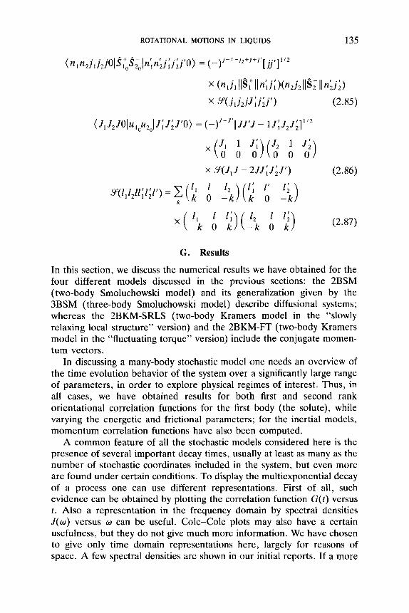
x ( 11 1 1 ; ) ( 12 G) - k O k - k O k
(2.85)
(2.86)
(2.87)
G . Results
In this section, we discuss the numerical results we have obtained for the four different models discussed in the previous sections: the 2BSM (two-body Smoluchowski model) and its generalization given by the 3BSM (three-body Smoluchowski model) describe diffusional systems; whereas the 2BKM-SRLS (two-body Kramers model in the “slowly relaxing local structure” version) and the 2BKM-FT (two-body Kramers model in the “fluctuating torque” version) include the conjugate momen- tum vectors.
In discussing a many-body stochastic model one needs an overview of the time evolution behavior of the system over a significantly large range of parameters, in order to explore physical regimes of interest. Thus, in all cases, we have obtained results for both first and second rank orientational correlation functions for the first body (the solute), while varying the energetic and frictional parameters; for the inertial models, momentum correlation functions have also been computed.
A common feature of all the stochastic models considered here is the presence of several important decay times, usually at least as many as the number of stochastic coordinates included in the system, but even more are found under certain conditions. To display the multiexponential decay of a process one can use different representations. First of all, such evidence can be obtained by plotting the correlation function G ( t ) versus t. Also a representation in the frequency domain by spectral densities J ( w ) versus w can be useful. Cole-Cole plots may also have a certain usefulness, but they do not give much more information. We have chosen to give only time domain representations here, largely for reasons of space. A few spectral densities are shown in our initial reports. If a more
136 ANTONINO POLIMENO A N D JACK H . FREED
detailed description is required, the best way to proceed seems to be the analysis of the dominant kinetic constants (i.e., eigenvalues of the time evolution operator), contributing significantly to the decay process (see below). The correlation function G(t ) can be written in terms of the eigenvalues hi of the time evolution operator according to the following expansion:
G(t) = c w i exp(-Ait) i
(2.88)
where each eigenvalue hi has a weight w i . In all the table entries we show the set of eigenvalues having weights larger than or equal to a cut-off value E . A measure of the overall correlation time of the process (i.e., the best approximation to a single exponential decay constant) is given, calculated as the zero frequency value of the spectral density.
It is interesting to investigate the eigenvectors corresponding to the dominant eigenvalues in a few cases. From the explicit expansion over the basis functions used for the matrix representation of the operator, one can obtain insight into the kind of motion represented by the ith mode (e.g., one can decide if it is mainly the isolated motion of the first body or if the solvent degrees of freedom are involved). Also, it is possible to gain information on the truncation criteria with respect to the different quantum numbers. This is particularly useful in dealing with models with more than three relevant (i.e., nondiagonal) quantum numbers.
1 . Computational Procedures
As pointed out above, the numerical algorithm with which we have chosen to evaluate the eigenvalues and eigenvectors of the many-body stochastic operators, and to compute the temporal decay of a given correlation function G(t) , consists of: (1) determining a suitable set of basis functions via standard angular momentum techniques; (2) obtaining the matrix representation r of the symmetrized operator, and the initial vector v; (this vector is calculated as the product of the matrix representa- tion M of the observable function and the vector vo, which represents Pi; , cf. Eq. (2.26)); ( 3 ) applying a real symmetric implementation of the Lanczos algorithm (for Hermitean operators) or a complex symmetric one (for non-Hermitean cases) to transform r into tridiagonal form T; (4) obtaining from T, by straightforward diagonalization of the eigen- value spectrum, and computing the temporal decay of G( t ) (alternatively one can directly calculate the spectral density J ( o ) using a continued fraction expansion [50,42]); ( 5 ) determining the eigenvectors correspond- ing to some eigenvalues (see below).
In this subsection, we wish to clarify some technical details concerning the computational procedure. One of the most serious difficulties one has

ROTATIONAL MOTIONS IN LIQUIDS 137
to deal with when considering a many-body operator is how to check the internal consistency of the expressions. After all, when considering a 2BKM one has to solve a partial differential equation with 12 variables (i.e., the dimension of the phase space), and this is by no means a straightforward task. First of all, one requires a test of the algebraic formulas that give r, vo, and v. Even though the procedures are clear, and based on the systematic usage of the Wignert-Eckart theorem, the large numbers of degrees of freedom involved, means possible algebraic mistakes that may be hard to find. For this purpose, we have found it very useful to check our algebraic manipulations made by hand, using standard computer algebra software packages such as Reduce [55] and Mathematica [56]. We did not write complete programs to perform all the algebraic steps; rather we checked separate parts of the calculation.
Another very useful way of testing our results has been to use two independent routes to numerically evaluate vo. The first route is reviewed in Appendix C. It consists of the direct evaluation of the vector elements in the coupled basis which largely involves numerical integration of the function Pa:. This direct approach is convenient for the case of rotation- al invariance which is characteristic of the physical systems we have studied. A second route has previously been recommended by Moro and Freed [50] and Schneider and Freed [42]. They consider the following expression
lim [sI + r]vo = c (2.89) s4n+
where c is an arbitrary vector with a component along vo. Equation (2.89) follows from the fact that P:i* is the unique stationary solution of the symmetrized operator f (i.e., the eigenvector of zero eigenvalue). One solves it for v", by using some efficient algorithm for large linear systems (e.g., the conjugate gradient method). Note that the calculation of vo by Eq. (2.89) involves the direct use of r. Since the formulation of r is algebraically the most challenging step, we regarded agreement of vo obtained by both methods as largely a confirmation of a correctly expressed r (as well as a reliable v"). In all cases we succeeded with this test to within appropriate numerical round-off error.
When one is reasonably sure of the algebraic formulas and programs, it is still necessary to check the convergence of each calculation, both with respect to the number of basis functions used (i.e., the dimension N of r) and the number of Lanczos steps (i.e., the dimension n of T). Although one can use sophisticated pruning procedures in order to minimize N [51], we have used the simple criterion of repeating the calculation by increas- ing both N and n until there is a relative variation less than 6 in all the dominant eigenvalues (i.e., all the eigenvalues having a relative weight
138 ANTONINO POLIMENO AND JACK H . FREED
larger than or equal to E ) . Usually S and E have both been chosen to equal
Finally, we discuss the procedure adopted to evaluate the eigenvector vA corresponding to a chosen eigenvalue A, since that is not normally delivered by the Lanczos algorithm. We have followed the suggestion of Cullum and Willoughby [57]. First, we evaluated the eigenvector v', of T in the basis of Lanczos vectors. This is an n-dimensional vector, which can be easily obtained by an expression similar to Eq. (2.89)
lim [(s + h)I + Tlv', = c (2.90) s+o+
One can now evaluate the Ritz eigenvector vA (i.e., the eigenvector of r in terms of its components in the original basis set) by simply premultiply- ing vl by the transformation matrix S
T = S"rS (2.91)
where S is the n X N matrix whose ith row is the ith Lanczos vector (within round-off errors, S"S is the n x n unit matrix). This last proce- dure is usually done by repeating the Lanczos tridiagonalization, so there is no need to store the n Lanczos vectors.
2. Two-Body Smoluchowski Model
We start with the two-body Smoluchowski model (2BSM); the details of the formulation (matrix and starting vector) are discussed in Section 1I.C. A stochastic system made of two spherical rotators in a diffusive (Smoluchowski) regime has been used recently to interpret typical bifur- cation phenomena of supercooled organic liquids [40]. In that work it was shown that the presence of a slow body coupled to the solute causes unusual decay behavior that is strongly dependent on the rank of the interaction potential.
In all the 2BSM calculations presented here, the diffusion coefficient D , equals 1, which defines the unit of frequency (inverse time); whereas the diffusion coefficient for the solvent, D, varied from 10 (very fast solvent relaxation) to 1, 0.1, 0.01 (very slow solvent relaxation). In the D, = 10 case, one finds that the reorientation of the solute is virtually independent of the solvent; a projection procedure could easily be adopted in this case to yield a one-body Smoluchowski equation for body 1 with perturbational corrections from body 2. The temporal decay of the first and second rank correlation functions is then typically monoexponen- tial. When the solvent is relaxing slowly (i.e., D, is in the range 1-O.Ol), the effect of the large cage of the rapid motion of the probe becomes
ROTATIONAL MOTIONS IN LIQUIDS 139
increasingly important. The decay of the correlation functions of both ranks is already different from that of a single exponential for D, = 1, and for D, = 0.1 the biexponential behavior is characterized by significantly different decay rates, since the separation of timescales for the two bodies is large.
An analysis of the different effects of a first rank versus a second rank interaction is instructive. A second rank potential between the bodies generates an apparent “strong collision” effect; that is, the motion of the first body in the potential field of the slow solvent body is dominated by the jump rate between the two equivalent minima. Only correlation functions of odd parity are sensitive to this jump motion, so that if an averaged unique correlation time is computed, this is significantly modi- fied for the first rank case (i.e., 7,) with respect to the free diffusional motion (i.e., no coupling) regime. Thus, for a fairly large range of parameters, the ratio r 1 / T 2 is lower than 3 (which is the typical value for a purely diffusive description) and often very close to 1 (typical of a strong collision description). When the potential is first rank, there is no comparable “jump” motion, and the ratio 7 / T is always equal to or larger than 3. In other words, a second rank interaction potential (i.e., u2 ZO) causes the solute (usually the faster body) to reorient in the instantaneous cage induced by the solvent (the slower body) or to jump to the other potential minimum. In this way, a two-body small-step diffusion model can exhibit features that are typical of a one-body-strong coffision description [58].
The numerical results are collected in Tables I1 and 111 (respectively, for first rank and second rank correlation functions for a first rank interaction potential) and Tables IV and V (second rank potential). Each entry is defined for a value of the potential parameter ( u , or u , ) and a value of the diffusion coefficient of the second body ( D 2 ) . The column on the left contains the zero-frequency spectral density or autocorrelation time
1.
+ia
71.2 = dtG1.2 = 5 1 . m (2.92)
(note again that the subscript 1, 2 refers to both T~ and T ~ , etc.), whereas the column on the right contains the dominant eigenvalue(s) of the process: for each mode A; the corresponding weight wi is given in parentheses.
Let us consider Table I1 in detail. When the solvent body is fast ( D , = lo), the only effect on the rotational correlation time T~ for an increasing tight interaction with the probe is a modest variation (going from 0.5 for u 1 = 0 to 0.53 for u , = 4). The solvent readjusts itself rapidly
Y
b
0
TA
BL
E I
1 2B
SM
: Fi
rst
Ran
k C
orre
lati
on T
imes
(L
eft
Col
umn)
, D
omin
ant
Eig
enva
lues
(R
ight
Col
umn)
" an
d So
me
of t
he
Cor
resp
ondi
ng E
igen
vect
orsb
D2
"1
10.0
1 .o
0.
0 0.
500
2.00
0(1.
000)
0.
500
2.00
0 (1
,000
) 0.
500
1.0
0.50
6 1.
970
(0.9
97)
0.55
5 1.
500
(0.6
50)
0.99
9
2.0
0.51
9 1.
919
(0.9
96)
0.66
5 1.
251
(0.7
63)
1.98
0
3.0
0.52
9 1.
883
(0.9
96)
0.75
7 1.
139
(0.8
31)
2.81
2
4.0
0.53
4 1.
863
(0.9
96)
0.81
5 1.
089
(0.8
70)
3.38
0
2.86
5 (0
.340
)
4.15
3 (0
.274
)
5.82
9 (0
.156
)
7.76
5 (0
.119
)
0.1 2.00
0 (1
.000
) 0.
500
0.19
7 (0
.118
) 5.
410
2.19
0 (0
.869
) 0.
191
(0.3
34)
14.9
7 2.
725
(0.6
31)
0.18
8 (0
.504
) 23
.11
3.51
5 (0
.448
) 0.
186
(0.6
12)
28.7
4 4.
469
(0.3
43)
0.01
2.00
0 (1
.000
) 0.
019
(0.0
96)
2.16
0 (0
.762
) 0.
019
(0.2
92)2
a 2.
603
(0.5
71)2
h 0.
019
(0.4
56)
3.28
1 (0
.428
) 0.
019
(0.5
60)*
' 4.
130
(0.3
561'
d
Eig
enva
lue
2a
Eig
enva
lue
2b
Eig
enva
lue
2c
Eig
enva
lue
2d
lc,l'
J
l J
, k,
IZ
J,
JZ
Ic,IZ
Jl
J
2
Ic,IZ
J
l J
,
0.76
1 0
1 0.
003
0 1
0.48
1 0
1
0.51
2 1
0 0.
077
1
0 0.
705
1 0
0.14
2 1
0 0.
245
1
2 0.
146
1 2
0.23
7 1
2 0.
275
1 2
0.12
9 2
1 0.
006
2 1
0.03
6 2
1 0.
037
2 1
0.08
1 2
3 0.
008
2 3
0.01
6 2
3 0.
053
2 3
0.01
7 3
2 0.
001
3 2
0.00
4 3
2 0.
012
3 4
0.00
5 3
4 0.
004
4 3
"The
se a
re c
alcu
late
d fo
r D
, = 1
(w
hich
def
ines
the
fre
quen
cy s
cale
) fo
r in
crea
sing
fir
st r
ank
pote
ntia
l co
uplin
g. F
or e
ach
'J i
s co
nsta
nt a
nd e
qual
to
1.
dom
inan
t ei
genv
alue
the
rel
ativ
e w
eigh
t is
giv
en (
in p
aren
thes
es).
TA
BL
E I1
1 2B
SM:
Seco
nd R
ank
Cor
rela
tion
Tim
es (
Lef
t C
olum
n),
Dom
inan
t E
igen
valu
es (
Rig
ht C
olum
n)”
and
Som
e of
the
C
orre
spon
ding
Eig
enve
ctor
sb
02
ui
10.0
1 .o
0.
1 0.
01
0.0
0.16
7 6.
000(
1.00
0)
0.16
7 6.
000
(1.0
00)
1.0
0.16
8 5.
910(
0.99
4)
0.17
5 3.
805
(0.1
97)
6.29
7 (0
.464
) 6.
632
(0.3
27)
2.0
0.17
1 5.
756
(0.9
90)
0.19
6 3.
532
(0.4
27)
7.16
0 (0
.376
) 8.
194
(0.1
52)
3.0
0.17
5 5.
650
(0.9
89)
0.21
7 3.
353
(0.5
72)
8.49
9 (0
.319
) 10
.45 (
0.07
2)
4.0
0.17
7 5.
591
(0.9
88)
0.23
4 3.
249
(0.6
60)
10.1
7 (0
.268
) 13
.34
(0.0
36)
0.16
7 6.
000
(1.0
00)
0.18
7 0.
591
(0.0
06)
2.40
4 (0
.067
) 6.
186
(0.8
95)
0.26
9 0.
575
(0.0
56)
2.97
5 (0
.175
) 6.
738
(0.6
90)
0.40
4 0.
565
(0.1
45)
3.81
3 (0
.281
) 7.
647
(0.4
70)
0.55
0 0.
559
(0.2
44)
4.80
5 (0
.333
) 8.
898
(0.2
93)
0.16
7 6.
000(
1.00
0)
0.24
4 0.
059
(0.0
04)
2.18
6 (0
.062
) 6.
163
(0.8
45)
0.83
8 0.
059
(0,0
39)’
” 2.
891
(0.0
28)3
h 6.
625
(0.5
00)“
2.
027
0.05
9 (0
,101
) 3.
319
(0.2
37)
7.36
4 (0
.258
) 3.
422
0.05
9 (0
.195
)’d
4.16
9 (0
.301
)”
8.35
0 (0
.134
)”
Eig
enva
lue
3a
Eig
enva
lue
3b
Eig
enva
lue
3c
Eig
enva
lue
3d
Eig
enva
lue
3e
Eig
enva
lue
3f
Id
J,
Jz
IC,I
Z
J,
J2
IC,l
2
J,
J,
lc,1
2 Jl
J
?
IC,I
Z
J,
J,
lC,l
2
Jl
J*
0.76
1 0
2 0.
009
0 2
0.05
5 1
1 0.
481
0 2
0.00
1 0
2 0.
102
1 1
0.09
4 1
1 0.
694
1 1
0.00
3 1
3 0.
172
1 1
0.46
7 1
1 0.
129
1 3
0.13
0 1
3 0.
241
1 3
0.63
0 2
0 0.
245
1 3
0.29
0 1
3 0.
294
2 0
0.00
3 2
0 0.
026
2 0
0.26
5 2
2 0.
019
2 0
0.08
8 2
0 0.
009
2 2
0.00
4 2
2 0.
011
2 2
0.02
1 2
4 0.
026
2 2
0.03
1 2
2 0.
390
2 4
0.00
1 2
4 0.
015
2 4
0.01
8 3
1 0.
045
2 4
0.09
0 2
4 0.
028
3 1
0.00
1 3
1 0.
005
3 3
0.00
2 3
3 0.
014
3 1
0.03
5 3
5 0.
004
3
5 0.
002
3 3
0.00
4 4
2 0.
012
3 5
0.00
6 4
6
“The
se ar
e ca
lcul
ated
for
D, =
1 fo
r in
crea
sing
firs
t ra
nk p
oten
tial
coup
ling.
For
eac
h do
min
ant
eige
nval
ue th
e re
lativ
e w
eigh
t
’5 i
s co
nsta
nt a
nd e
qual
to
2.
is g
iven
(in
par
enth
eses
).

TA
BL
E I
V
2BSM
: Fi
rst
Ran
k C
orre
lati
on T
imes
(L
eft
Col
umn)
, D
omin
ant
Eig
enva
lues
(R
ight
Col
umn)
" an
d So
me
of t
he
Cor
resp
ondi
ng E
igen
vect
orsb
1.0
~~
0.1
0.01
0.0
0.50
0 2.
000(
1.00
0)
0.50
0 2.
000
(1.0
00)
0.50
0 1.
0 0.
505
1.97
9 (0
.999
) 0.
534
1.83
5 (0
.973
) 0.
608
2.0
0.51
8 1.
926
(0.9
61)
0.64
1 1.
487
(0.9
45)
1.06
8
3.0
0.53
1 1.
877
(0.9
98)
0.77
2 1.
226
(0.9
37)
2.02
7
4.0
0.54
0 1.
849
(0.9
98)
0.86
9 1.
097
(0.9
47)
3.26
3
9.36
8 (0
.045
)
12.3
9 (0
.041
)
16.6
3 (0
.031
)
2.00
0 (1
.000
) 1.
291
(0.6
37)
3.10
8 (0
.356
) 0.
693
(0.6
94)
4.42
4 (0
.275
) 0.
387
(0.6
94)
6.30
5 (0
.158
) 0.
256
(0.8
31)
8.75
3 (0
.102
)
0.50
0 2.
000
(1.0
00)
0.64
2 1.
064
(0.4
94)
2.81
1 (0
.491
) 1.
353
0.49
5 (0
.627
)'"
4.04
0 (0
.337
)Jb
3.52
2 0.
210
(0.7
31)
5.77
4 (0
.224
) 9.
167
0.08
7 (0
.801
)''
8.02
5 (0
.143
)4d
Eig
enva
lue
4a
Eig
enva
lue
4b
Eig
enva
lue
4c
Eig
enva
lue
4d
k,IZ
J
, J
2
IC,I
Z
J,
J*
Ic,1
2 J
, J
2
Ic
f
J,
J,
0.32
1 1
0 0.
640
1 0
0.26
3 1
0 0.
610
1 0
0.62
0 1
2 0.
331
1
2 0.
516
1
2 0.
310
1
2 0.
025
3 2
0.01
5 3
2 0.
086
3 2
0.03
5 3
2 0.
034
3 4
0.01
2 3
4 0.
112
3 4
0.02
7 3
4 0.
010
5 4
0.00
9 5
4 0.
012
5 6
0.00
6 5
6
"The
se a
re c
alcu
late
d fo
r D
, = 1
for
inc
reas
ing
seco
nd r
ank
pote
ntia
l co
uplin
g. F
or e
ach
dom
inan
t ei
genv
alue
the
rel
ativ
e w
eigh
t is
giv
en (
in p
aren
thes
es).
'J i
s co
nsta
nt a
nd e
qual
to
1.

TA
BL
E V
2B
SM
: S
econ
d R
ank
Cor
rela
tion
Tim
es (
Lef
t C
olum
n),
Dom
inan
t E
igen
valu
es (
Rig
ht C
olum
n)”
and
Som
e of
the
C
orre
spon
ding
Eig
enve
ctor
s’
u,
10.0
1 .o
0.
1 0.
01
0.0
0.16
7 6.
000(
1.00
0)
0.16
7 6.
000(
1.00
0)
0.16
7 1 .
O 0.
168
5.93
6 (0
.998
) 0.
178
4.78
5 (0
.595
) 0.
252
7.56
7 (0
.386
)
2.0
0.17
2 5.
777
(0.9
96)
0.20
9 3.
899
(0.7
09)
0.50
6 10
.0 (0
.268
)
3.0
0.17
6 5.
631
(0.9
95)
0.24
6 3.
414
(0.7
92)
0.80
9 13
.43
(0.1
74)
4.0
0.17
9 5.
546(
0.99
5)
0.17
3 3.
192(
0.84
6)
1.05
0
6.00
0 (1
,000
) 0.
167
0.59
3 (0
.059
) 0.
981
5.93
9 (0
.653
) 7.
327
(0.1
48)
0.57
7 (0
.230
) 3.
402
6.54
8 (0
.565
) S
.laO
(0.1
07)
0.56
3 (0
.412
) 6.
303
7.94
9 (0
.365
) 9.
470
(0.1
20)
0.55
4 (0
.561
) 8.
648
10.0
6 (0.
216)
11
.54(
0.13
8)
6.00
0(1.
000)
0.
059
(0.0
50)
5.56
5 (0
.323
) 6.
042
(0.2
74)
0.05
9 (0
. 190
)5”
6.04
3 (0
.258
) 6.
679
(0.3
57)5
b 0.
059
(0.3
69)
7.19
8 (0
.151
) 8.
019
(0.3
32)
0.05
9 (0
.511
)5‘
9.99
6 (0
.298
)5d
L
P
w
~~
~ ~~
~~
~
Eig
enva
lue
5a
Eig
enva
lue
5b
Eig
enva
lue
5c
Eig
enva
lue
5d
lc,IZ
J
, Jz
I
Cf
J
, Jz
lc
,ll
J,
Jz
lcf
J
, J
2
0.78
9 0
2 0.
002
0 2
0.47
4 0
2 0.
006
0
2 0.
040
2 0
0.33
9 2
0 0.
093
2 0
0.32
5 2
0
0.05
6 2
2 0.
085
2 2
0.13
2 2
2 0.
085
2 2
0.09
7 2
4 0.
550
2 4
0.22
6 2
4 0.
480
2 4
0.00
2 4
2 0.
008
4 2
0.02
0 4
2 0.
038
4 2
0.00
2 4
4 0.
013
4 6
0.01
7 4
4 0.
002
4 4
0.00
3 4
6 0.
034
4 6
0.05
7 4
6 0.
001
6 4
0.04
3 6
4 0.
001
6 6
“The
se a
re c
alcu
late
d fo
r D, = 1
for
inc
reas
ing
seco
nd r
ank
pote
ntia
l co
uplin
g. F
or e
ach
dom
inan
t ei
genv
alue
the
rel
ativ
e w
eigh
t is
give
n (i
n pa
rent
hese
s).
’J i
s co
nsta
nt a
nd e
qual
to
2.
144 ANTONINO POLIMENO AND JACK H . FREED
to the solute motion. For lower values of the diffusion coefficient of the solvent body, the decay of the correlation function is controlled by two dominant modes: one of them (the fast one) may be related to the rotational diffusion of the first body relative to the instantaneous orienta- tion of the solvent body, and the other one to the free rotational diffusion of the solvent body. One can see that for increasing potentials the process is more and more differentiated from the original free rotational diffusion (FRD), that is, the rotational diffusive motion of a spherical body in the absence of any coupling. The slow mode becomes more and more effective when the potential strength is increased (i.e., the weight goes from 0.096 for u , = 1 to 0.560 for u1 = 4, for D2 = 0.01). This is the cause of the dramatic increase of the autocorrelation time, since the solute rotation is heavily damped by the large cage.
The composition of the eigenvectors corresponding to the dominant modes is analyzed in two cases (D, = 0.01 and u , = 2, 4) in terms of the basis sets used in the representation of the time evolution operator (see Table 11). The square moduli of the coefficients c i , each of them representing the contribution of the basis set function labeled by the collective index A to the ith eigenvector, are shown together with the index A itself. In the present case, only the quantum numbers J , and J , are nondiagonal, while the total angular momentum quantum number J is a constant, and it is equal to 1 (2) for first (second) rank correlation functions. From the entry of Table I1 to the eigenvalue labeled 2a (D, = 0.01 and u1 = 2), one can see that the slow mode is largely a FRD of the solvent body ( I c i I 2 equal to 0.76 for J , = 0, J , = 1) with a small component of “dynamic interaction” between the two bodies ( lci12 equal to 0.14 for J , = 1, 5, = 2). From entry 2b it is seen that the fast mode is mostly due to FRD of the solute body ( l c i I 2 equal to 0.70 for J , = 1, J2 = 0), again with a dynamic interaction contribution (lci12 equal to 0.23 for J , = 1, J , = 2). The dynamic interaction becomes more important for the case of a tighter interaction ( u , = 4); cf. entries 2c and 2d.
Table I11 contains correlation times and dominant eigenvalues for a second rank observable in a first rank potential. There are still roughly two ranges of decay rates when the solvent body is slow (D, 5 1). The slower range is mostly due to the FRD of the solvent body, while the faster one is described by motions of the solute body and/or dynamic interactions. This faster decay is hardly described by a single frequency, unlike the case of a first rank correlation function. Rather, it is controlled by a few eigenvalues of the same order of magnitude. Thus for D, = 0.01 and u1 = 2 the slow mode, entry 3a in Table 111, is largely described by a J , = 0, 5, = 2 term; the fast mode 3b is’mostly due to dynamic interactions (5, = 1, J2 = 1 and J , = 1, J , = 3 are the important terms); and the fast
ROTATIONAL MOTIONS IN LIQUIDS 145
mode 3c is mainly due to FRD of the solute ( J , = 1, J2 = 0 is dominant). Dynamic interaction terms are more important in the eigenvectors when the potential is stronger ( u l = 4): see entries 3d (similar to 3a), 3e (similar to 3b) and 3f (similar to 3c), and note that mode 3e, which is dominated by dynamic interactions, is now heavily weighted in the correlation function.
When a second rank potential is considered, the previous description must be modified, particularly when odd rank autocorrelation functions are involved, as we have pointed out above. We present results here that confirm our previous interpretation [40]. In Table IV we show correlation times and eigenmodes for a first rank observable. As in Table 11, two dominant modes are present for D, 5 1; the fast one is again a FRD of the solute body, whereas the slow one is a thoroughly “mixed” nature (i.e., dynamic interactions), and may be loosely related, for very slow cages, to the jump motion of body 1 from one metastable orientation to another (cf. the cases in Table IV for D, = 0.01, u, = 2 and u2 = 4).
Finally, results on second rank correlation functions for a second rank potential are collected in Table V. The situation is now very similar to the corresponding set of data for a first rank potential (Table 111), since even rank correlation functions are not sensitive, for symmetry reasons, to jump motions. The slow mode is then again mostly due to the FRD of the larger solvent body while the fast modes are mainly dominated by motions of the first body (cf. the entries for D, = 0.01, u2 = 2 and 4 in Table V). Note that other faster eigenvalues are present, with smaller weights, whose nature is mostly mixed, but are not listed in the table. Their individual contribution to the overall decay of the correlation function is small, but their cumulative weights may be around 0.1-0.3 or even more.
In Figs. 2a-d, we show the time decay of the first rank correlation function G , ( t ) for a first rank potential. In Fig. 2a results for different values of u , for D, = 10 are shown (they correspond to the first column in Table 11). Observe that even for large potentials the effect of the light solvent body is negligible. For intermediate values of D, (cf. Figs. 2b and 2c) the contribution of the slow decay mode is more effective. A complete separation of time scales is evident in Fig. 2d ( D , = 0.01). Similar behavior is obtained in the case of a second rank potential (Figs. 4a-d) . Finally, the same features are observed in the case of second rank correlation functions G2(t) both for a first rank potential (Figs. 3a-d) and a second rank one (Figs. 52-4, although the sensitivity of second rank correlation functions to the size of the solvent body seems to be less pronounced than for first rank correlation functions (compare for exam- ple Fig. 2c with Fig. 3c).
146 ANTONINO POLIMENO AND JACK H. FREED
4 7
v A u 2 x 1 :m; 0
.. 0
9 d:. 0
0
1 .o 2.0
I
0.0 2.0 4.0 6.0 8.0 10.0 t
(b )
4 7
0.0 2.0 4.0 6.0 8.0 10.0 t
(d)
Figure 2. 2BSM First rank correlation functions for a first rank potential coupling: - u = o . __- - u = 1. -.-.- , ~ , = 2 ; ' . . . . , ~ , = 3 ; - . . - . . - , ~ , = 4 . ( a )Dz=10 ; (6 )
, I , , I 1
D , = 1; ( c ) D, = 0.01. The unit of time in Figs. 2-7 has been taken by setting 0;' = 1 .
From the strictly computational point of view, we may note that all the computations were made with truncation parameters J1,,, , J2,,, ranging from 4 to 8; the number of Lanczos steps necessary to achieve conver- gence (with respect to the correlation times and the dominant eigen- values) was usually less than 50.
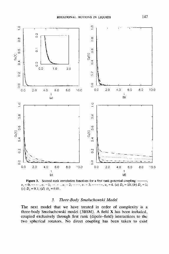
ROTATIONAL MOTIONS IN LIQUIDS 147
9 c
c9 0
'4 0 ,-. c v
(3" 2
N 0
0
0.0 1 .o 2.0
0.0 2.0 4.0 6.0 8.0 10.0 t (a)
9 - c9 0
'4 0
,--. c v N
(3
t 0
2 - s ,
\ " \
- L- 7 - _ . 0
0 0 2 0 4 0 6 0 8 0 100
0.0 2.0 4.0 6.0 8.0 10.0 t
(b )
\ . . -
. . . . . . . . . . . . . . . . . . . . . . . , ' . . . . . . . . . . . . . . .
8 1 ( \ ,
0.0 2.0 4.0 6.0 8.0 10.0
Figure 3. Second rank correlation functions for a first rank potential coupling: -, " = o . _ _ _ _ u = 1 . _._._ u = 2 . . . . . . u = 3 . _.._.._ , u , = 4. ( a ) D, = 10; ( b ) D, = 1; ( c ) D, = 0.1; ( d ) D, =0.01.
I , 3 1 9 3 1 2 3 1 1
3. Three-Body Smoluchowski Model
The next model that we have treated in order of complexity is a three-body Smoluchowski model (3BSM). A field X has been included, coupled exclusively through first rank (dipole-field) interactions to the two spherical rotators. No direct coupling has been taken to exist
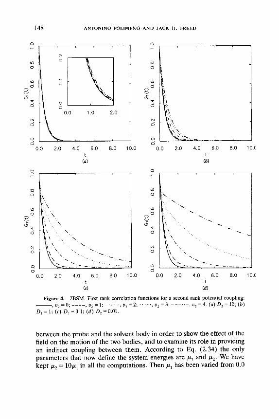
148 ANTONINO POLIMENO AND JACK H. FREED
0.0 2.0 4.0 6.0 8.0 10.0 t
(a)
0 0.0 2.0 4.0 6.0 8.0 10.0
t (C)
0.0 2.0 4.0 6.0 8.0 10.C t
(b)
0.0 2.0 4.0 6.0 8.0 10.C t
(d)
Figure 4. ZBSM. First rank correlation functions for a second rank potential coupling: __ t 2 u =o. 3 _ _ _ _ , , " 7 _.-.- , ~ , = 2 ; . . . . . , ~ , = 3 ; - . . - . . - , ~ , = 4 . (a )D2=10; ( b ) D, = 1; (c) D, = 0.1; ( d ) D , = 0.01.
between the probe and the solvent body in order to show the effect of the field on the motion of the two bodies, and to examine its role in providing an indirect coupling between them. According to Eq. (2.34) the only parameters that now define the system energies are p, and p2. We have kept p2 = lopl in all the computations. Then p1 has been varied from 0.0
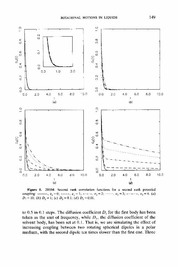
ROTATIONAL MOTIONS IN LIQUIDS 149
\ . , - .
- . . - . .
. . . . . . - . - . . - . . . . ..... .... . . . . . . . - . . - .
.... . . . . . .
....
- \
9 T-
2
x x z
+ v
s
9 0
0.0 1 .o 2.0
L 0.0 2.0 4.0 6.0 8.0 10.0
t (a)
I
\
/
\ \ '.,', . - . . (' ;. :: :.: : .-, - :,.-,,, . - , - _ .
0.0 2.0 4.0 6.0 8.0 10.0 t
(C)
0.0 2.0 4.0 6.0 8.0 10.0 t
(b )
2
x 2
2
x
- c v
s
- 0.0 2.0 4.0 6.0 8.0 10.0
t (d)
Figure 5. 2BSM. Second rank correlation functions for a second rank potential coupling: - v = o . ---- v = 1' -.-.- . v 2 = 2 : . . . . . v z = 3 ; -..- ..-( v2=4. ( a ) , 2 1 9 2 1
D, = 10; ( b ) D, = 1; (c) D, = 0.1; ( d ) D2 = 0.01.
to 0.5 in 0.1 steps. The diffusion coefficient D , for the first body has been taken as the unit of frequency, while D,, the diffusion coefficient of the solvent body, has been set at 0.1. That is, we are simulating the effect of increasing coupling between two rotating spherical dipoles in a polar medium, with the second dipole ten times slower than the first one. Three
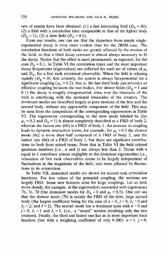
150 ANTONINO POLIMENO AND JACK H . FREED
sets of results have been obtained: ( 1 ) a fast interacting field (D, = 10); (2) a field with a correlation time comparable to that of the lighter body (D, = 1); (3) a slow field (D, = 0.1).
From our results, one can see that the departure from simple single- exponential decay is even more evident than for the 2BSM case. The correlation functions of both ranks are greatly affected by the motion of the field, so that a third decay constant is almost always necessary to fit the decay. Notice that the effect is most pronounced, as expected, for the case D , = 0.1. In Table VI the correlation times and the most important decay frequencies (eigenvalues) are collected for each set of values of p, and D,, for a first rank rotational observable. When the field is relaxing rapidly ( D , = 10, first column), the system is always biexponential for a significant coupling ( p1 2 0.2): that is, the fast third body just provides an effective coupling between the two bodies. For slower fields (D, = 1 and 0.1) the decay is roughly triexponential, since now the timescale of the field is interfering with the motional timescales of the rotators. The dominant modes are described largely as pure motions of the first and the second body, without any appreciable component of the field. This may be seen from the composition of the corresponding eigenvectors in Table VI. The eigenvector corresponding to the slow mode labeled 6a (for p1 = 0.2 and D, = 1) is almost completely described as a FRD of body 2, whereas the fastest one (6b) is a FRD of body 1. An increase in coupling leads to dynamic interaction terms; for example, for p, = 0.5 the slowest mode (6c) is more than half composed of a FRD of body 2, and the fastest one (6d) of a FRD of body 1, but there are significant contribu- tions to both from mixed terms. Note that in Table VI the field related quantum numbers (i.e., n and j ) are always less than 2. Terms with n equal to 1 contribute almost negligibly to the dominant eigenmodes; i.e., relaxation of first rank observables seems to be largely independent of fluctuations in the magnitude of the field, and more affected by fluctua- tions in its orientation.
In Table VII, numerical results are shown for second rank correlation functions. For low values of the potential coupling, the motions are largely FRD. Some new features arise for large couplings. Let us look more closely, for example, at the eigenvectors associated with eigenvalues 7b, 7c, 7d (the dominant modes for D, = 1 and pl = 0.5). One can see that the slowest mode (7b) is mainly the FRD of the slow, large second body (the largest coefficient being for the case of n = 0, j = 0, J , = 0 and J2 = 2; and J = 2). The second mode has a dominant term with n = 0 and j = 0, J , = 1 and J2 = 1, (i.e., a “mixed” motion involving only the two rotators). Finally, the third and fastest one has as its most important basis function (but with a weighting coefficient of only 0.380): n = 1, j = 0,
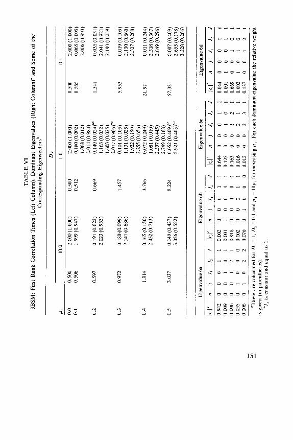
TA
BL
E V
I 3B
SM
: F
irst
Ran
k C
orre
lati
on T
imes
(L
eft
Col
um
n),
Dom
inan
t E
igen
valu
es (
Rig
ht
Col
um
n)"
an
d S
ome
of t
he
Cor
resp
ondi
ng E
igen
vect
ors'
D.,.
Pl
10.0
1 .
0 0.
1
0.0
0.50
0 2.
000
(1.0
00)
0.50
0 2.
000(
1.00
0)
0.50
0 2.
000
(1,0
00)
0.1
0.50
6 1.
999
(0.9
47)
0.51
2 0.
180
(0.0
02)
0.56
5 0.
065
(0.0
05)
1.06
8 (0.
012)
2.
006
(0.9
93)
2.01
4 (0
.984
) 0.
2 0.
597
0.19
1 (0
.022
) 0.
669
0.14
0 (0
.024
)'"
1.34
1 0.
035
(0.0
31)
1.16
3 (0
.032
) 2.
041
(0.9
21)
1.60
3 (0
.025
) 2.
193
(0.0
39)
2.07
7 (0
.905
)Yb
0.10
1 (0
.105
) 5.
933
0.01
9 (0
.105
) 2.
141
(0.8
86)
1.13
1 (0
.025
) 7.
130
(0.6
60)
1.92
2 (0
.190
) 2.
327
(0.2
08)
2.25
5 (0
.656
) 0.
4 1.
814
0.16
5 (0
.150
) 3.
766
0.07
2 (0
.249
) 21
.97
0.01
1 (0
.244
) 2.
452
(0.7
13)
1.08
1 (0
.010
) 2.
318
(0.3
67)
2.39
7 (0
.445
) 2.
649
(0.2
96)
2.74
9 (0
.168
) 0.
5 3.
037
0.14
9 (0
.437
) 8.
224
0.05
2 (0
.409
)''
57.3
3 0.
007
(0.4
09)
3.05
6 (0
.522
) 2.
Y21
(0.
403)
0d
2.69
5 (0
.178
) 3.
228
(0.2
66)
2.02
3 (0
.933
)
0.3
0.97
2 0.
180
(0.0
99)
1.45
7
Eig
enva
lue 6
a E
igen
valu
e 6b
Eig
enva
lue 6
c E
igen
valu
e 6d
lc,I
2
ti j
J,
Jz
J (c
,I2
n
j J,
Jz
J
Ic,I
z n
j J,
J,
J
Ic,~'
n j
J,
J,
J
0.94
2 0
0 0
1 1
0.00
2 0
0 0
1 1
0.64
4 0
0 0
1 1
0.04
4 0
0 0
1 1
0.00
9 0
0 1
0 1
0.00
1 1
0 0
1 1
0.12
5 0
0 1
0 1
0.00
1 1
0 0
1 1
0.00
6 0
0 1
2 1
0.91
8 0
0 1
0 1
0.16
3 0
0 1
2 1
0.66
9 0
0 1
0 1
0.03
5 0
1 0
0 0
0.00
2 0
0 2
1 1
0.01
6 0
0 2
1 1
0.00
2 1
0 1
0 1
0.00
6 0
1 0
2 2
0.07
0 0
1 0
0 0
0.01
2 0
0 2
3 1
0.13
7 0
0 1
2 1
"The
se a
re c
alcu
late
d fo
r D, = 1
. D,
= 0
.1 a
nd p
, =
lo
p, f
or i
ncre
asin
g p
, . F
or e
ach
dom
inan
t ei
genv
alue
the
rel
ativ
e w
eigh
t
'J,
is co
nsta
nt a
nd e
qual
to
1.
L
Y
m
is g
iven
(in
par
enth
eses
).
c
v1
N
TA
BL
E V
II
3BSM
: Se
cond
Ran
k C
orre
lati
on T
imes
(L
eft
Col
umn)
, D
omin
ant
Eig
enva
lues
(R
ight
Col
umn)
” an
d So
me
of t
he
Cor
resp
ondi
ng E
igen
vect
orsh
Dx
PI
10.0
1 .o
0.
1
0.0
0.16
7 6.
000(
1.00
0)
0.16
7 6.
000
(1.O
OO
) 0.
167
6.00
0 (1
.000
) 0.
1 0.
167
5.99
4 (0
.996
) 0.
167
6.01
0 (0
.994
) 0.
167
6.00
6 (0
.994
) 0.
2 0.
170
2.21
8 (0
.013
) 0.
171
2.22
5 (0
.012
) 0.
176
0.08
6 (0
.001
) 6.
003
(0.9
78)
6.06
0 (0
.965
)?”
2.08
9 (0
.018
)
0.3
0.18
5 0.
541
(0.0
04)
0.19
7 0.
302
(0.0
05)
0.28
3 2.
335
(0.0
58)
2.39
8 (0
.033
) 6.
097
(0.9
03)
6.20
5 (0
.875
)
2.65
4 (0
.137
) 2.
589
(0.1
27)
6.38
2 (0
.698
) 6.
521
(0.6
69)
3.27
6 (0
.241
) 3.
039
(0.1
65)”
6.
969
(0.5
33)
7.08
8 (0
.344
)7d
0.4
0.24
0 0.
497
(0.0
22)
0.32
6 0.
214
(0.0
21)
1.06
8
0.5
0.38
3 0.
450
(0.0
94)
0.77
6 0.
156
(0.0
95)7
b 4.
220
6.04
1 (0
.930
) 0.
054
(0.0
05)
2.22
2 (0
.060
) 6.
108
(0.8
91)
0.03
3 (0
.030
) 2.
554(
0.12
9)
6.51
5 (0
.746
) 0.
022
(0.0
96)
3.17
3 (0
.232
) 7.
1 12
(0.4
56)
Eig
enva
lue 7
a E
igen
valu
e 7b
E
igen
valu
e 7c
E
igen
valu
e 7d
Ic,I
z n
j J,
J
?
J Ic
,Iz
n j
J,
J,
J Ic
,Iz
n j
J,
J,
J Ic
,Iz
n j
J,
J,
J
0.00
1 0
0
1 1
2 0.
586
0 0
0 2
2 0.
090
0 0
0 2
2 0.
006
0 0
0 2
2 0.
978
0 0
2
0 2
0.00
1 1
0 0
2 2
0.00
2 1
0 0
2 2
0.36
0 1
0 0
2 2
0.01
6 0
1 1
0
1 0.
162
0 0
1 1
2 0.
611
0 0
1 1
2 0.
008
0 0
1 1
2 0.
002
0 1
3 0
3 0.
119
0 0
1 3
2 0.
005
1 0
1 1
2 0.
106
1 0
1 1
2 0.
011
0 0
2 0
2 0.
124
0 0
1 3
2 0.
003
0 0
1 3
2 0.
011
0 0
2 2
2 0.
041
0 0
2 0
2 0.
029
1 0
1 3
2 0.
008
0 0
2 4
2 0.
008
0 0
2 2
2 0.
020
0 0
2 0
2 0.
054
0 1
0 1
1 0.
010
0 0
2 4
2 0.
010
1 0
2 0
2
“The
se a
re c
alcu
late
d fo
r D, =
1, D, = 0
.1 a
nd f
i2 =
lo&
, for
incr
easi
ng f
i,.
For
each
dom
inan
t eig
enva
lue
the
rela
tive
wei
ght
’5,
is co
nsta
nt a
nd e
qual
to
2.
is g
iven
(in
par
enth
eses
).
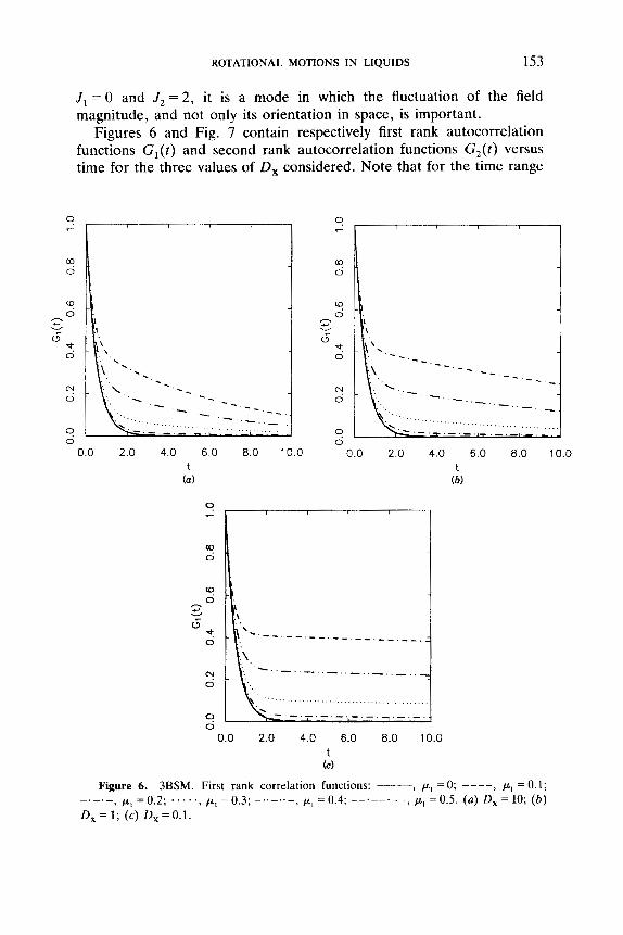
ROTATIONAL MOTIONS IN LIQUIDS 153
P,
\ '-.
J , = 0 and J2 = 2 , it is a mode in which the fluctuation of the field magnitude, and not only its orientation in space, is important.
Figures 6 and Fig. 7 contain respectively first rank autocorrelation functions G, ( r ) and second rank autocorrelation functions G2(r) versus time for the three values of D, considered. Note that for the time range
9 j a I I
0
0.0 2.0 4.0 6.0 8.0 10.0 0.0 2.0 4.0 6.0 8.0 10.0 t (a)
t (b )
0.0 2.0 4.0 6.0 8.0 10.0 t
(C)
Figure 6. 3BSM. First rank correlation functions: - p = O . ---- p =0.1; =0,2. ..... PI =0,3; -..-..- PI = 0.4; --. --. -- , p, = 0.5. (a ) D , = 10; ( b )
, I 9 , I
_.-._ ' 1
D , = 1 ; (c) D , =0.1.

154 ANTONINO POLIMENO AND JACK H. FREED
\:-.-.
Figure 7. 3BSM. Second rank correlation functions: ~ . I P =o. 3 ----, pI =0.1; , pI = 0.5. ( a ) D, = 10; ( b ) -.-._ I.L = 0.2. . . . . ., =0,3; -.._.._ = 0.4;
D, = 1; ( c ) D, = 0.1 . I
considered (ten times the inverse of D l ) , first rank correlation functions are much more affected by a large coupling via the fluctuating field than are second rank functions. This is primarily due to the slow eigenvalues which are strongly dependent on yl. This drastically changes the long- time behavior of GI, such that T , for the first rank processes is much larger for large yl.
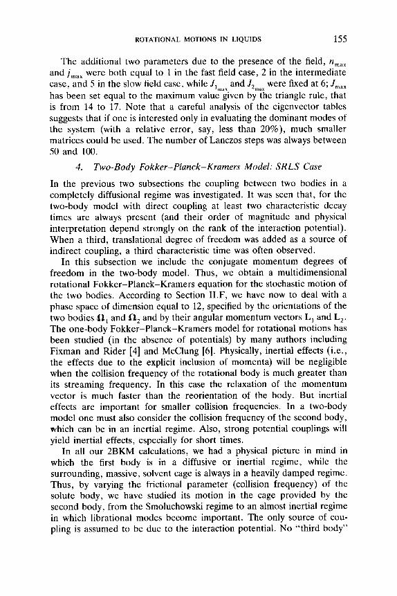
ROTATIONAL MOTIONS IN LIQUIDS 155
The additional two parameters due to the presence of the field, nmai and j , , , were both equal to 1 in the fast field case, 2 in the intermediate case, and 5 in the slow field case, while J , , , , and J2 m a x were fixed at 6; J,,, has been set equal to the maximum value given by the triangle rule, that is from 14 to 17. Note that a careful analysis of the eigenvector tables suggests that if one is interested only in evaluating the dominant modes of the system (with a relative error, say, less than 20%), much smaller matrices could be used. The number of Lanczos steps was always between 50 and 100.
4. Two-Body Fokker-Planck-Kramers Model: SRLS Case
In the previous two subsections the coupling between two bodies in a completely diffusional regime was investigated. It was seen that, for the two-body model with direct coupling at least two characteristic decay times are always present (and their order of magnitude and physical interpretation depend strongly on the rank of the interaction potential). When a third, translational degree of freedom was added as a source of indirect coupling, a third characteristic time was often observed.
In this subsection we include the conjugate momentum degrees of freedom in the two-body model. Thus, we obtain a multidimensional rotational Fokker-Planck-Kramers equation for the stochastic motion of the two bodies. According to Section II.F, we have now to deal with a phase space of dimension equal to 12, specified by the orientations of the two bodies 0, and 0, and by their angular momentum vectors L, and L,. The one-body Fokker-Planck-Kramers model for rotational motions has been studied (in the absence of potentials) by many authors including Fixman and Rider [4] and McClung [6]. Physically, inertial effects (i.e., the effects due to the explicit inclusion of momenta) will be negligible when the collision frequency of the rotational body is much greater than its streaming frequency. In this case the relaxation of the momentum vector is much faster than the reorientation of the body. But inertial effects are important for smaller collision frequencies. In a two-body model one must also consider the collision frequency of the second body, which can be in an inertial regime. Also, strong potential couplings will yield inertial effects, especially for short times.
In all our 2BKM calculations, we had a physical picture in mind in which the first body is in a diffusive or inertial regime, while the surrounding, massive, solvent cage is always in a heavily damped regime. Thus, by varying the frictional parameter (collision frequency) of the solute body, we have studied its motion in the cage provided by the second body, from the Smoluchowski regime to an almost inertial regime in which librational modes become important. The only source of cou- pling is assumed to be due to the interaction potential. No “third body”
156 ANTONINO POLIMENO AND JACK H . FREED
effects are included for simplicity, and the model can be regarded as a generalization of the “slowly relaxing local structure” (SRLS) models of Freed and co-workers [33,35].
Throughout this set of simulations, the unit of frequency has been chosen as the streaming frequency of body 1, that is, o; = 1; the ratio between the moments of inertia has been set equal to 10, that is, Z2/Zl = 10, so that the streaming frequency of the second body is given by oS, = l/m. Finally, the collision frequency oi of body 2 has been maintained at 100. The only parameters varied were the collision fre- quency of body 1, w ; (for values of 50 (damped case), 5 (intermediate case), 0.5 (inertial case)). The computations were performed both for a first rank potential (u , = 0, 1 , . . . , 3 ) and for a second rank potential (u2 = 0, 1, . . . ,3 ) . Orientational correlation functions of rank 1 and 2 for body 1 have been computed; also, correlation functions for the reorienta- tion of the conjugate momentum L, have been evaluated.
Table VIII contains the autocorrelation times and the dominant modes for first rank correlation observables. Note that in this table, and in the following tables for Kramers models, the eigenvalues and their weights are complex numbers (but the real part of any eigenvalue is nonnegative). In this and succeeding tables we write the real and imaginary parts for each and we use the convention of placing a bar over the first figure of a negative number. Since the correlation function must be real, each complex eigenvalue is accompanied by irs conjugate, which is not shown in the table.
As was the case in the 2BSM, a slow eigenmode (equal to twice the diffusion coefficient of the solvent body) is always present. It represents the FRD of the large cage in the diffusive regime. The only exception is for zero coupling (u , =0) where the model reduces to a one-body case (that is completely equivalent to the spherical rotational Kramers case treated by McClung). The motion of the solute body is responsible for the other fast modes whether in the diffusive regime (of = 50), the intermediate regime (of = 5 ) or the inertial regime (of = 0.5). In the last case there are eigenmodes with nonzero imaginary parts having a signifi- cant weight. These motions are of a librational kind. But there are also fast modes whose eigenvalues are purely real, and they correspond to solute modes that are largely diffusional (i.e., the coupling to angular momentum is not very significant). Thus the model seems to provide three different types of decay process: namely, a pure rotation of the solvent body (slow mode), a librational motion of the solute body (complex mode), and a fast reorientation of larger amplitude, more or less related to the FRD of the solute body.
Table IX gives the equivalent results for a second rank observable.
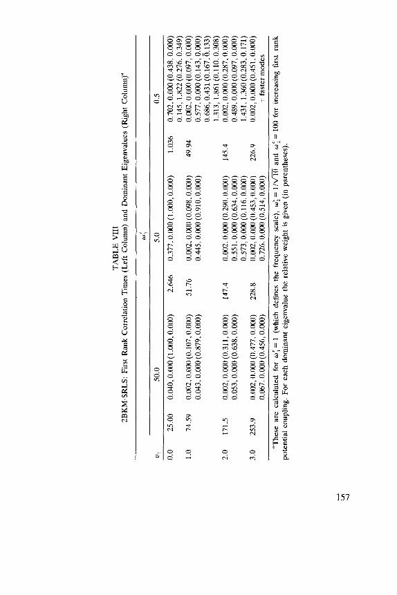
TA
BL
E V
III
2BK
M-S
RL
S: F
irst
Ran
k C
orre
lati
on T
imes
(L
eft
Col
umn)
and
Dom
inan
t E
igen
valu
es (
Rig
ht C
olum
n)"
0:
u1
50.0
5.
0 0.
5
0.0
25.0
0 0.040,0.000(1.000,0.000)
2.64
6 0.377,0.000(1.000,0.000)
1.03
6 0.
702,
0.00
0(0.
438,
0.00
0)
0.14
5, 1
.822
(0.2
76.0
.349
) 1.
0 74
.59
0.00
2,0.
000(
0.10
7.0.
000)
51
.76
0.00
2,0.
000(
0.09
8.0.
000)
49
.94
0.00
2,0.
000(
0.09
7.0.
000)
0.
043,
O.O
OO
(0.8
79,0
.000
) 0.
445,
0.00
0 (0
.910
,0.0
00)
0.57
7,0.
000
(0.1
43,0
.000
) 0.686,0.431(0.167,6.133)
1.313,1.861(0.110,0.308)
2.0
171.
5 0.
002,
0.00
0(0.
311,
0.00
0)
147.
4 0.
002,
0.00
0(0.
290.
0.00
0)
145.
4 0.
002,
0.00
0(0.
287,
0.00
0)
0.053,O.OOO (0.638,0.000)
0.55
1.0.
000
(0.6
34.0
.000
) 0.
489,
O.O
OO
(0.0
97,O
.OO
O)
0.573,0.000 (0
.116
.0.0
00)
1.43
1.1.
360
(0.2
83,0
.171
) 3.
0 25
3.9
0.00
2,0.
000(
0.47
7,0.
000)
22
8.8
0.002,0.000(0.453,0.000)
226.
9 0.
002,
0.00
0(0.
451,
0.00
0)
"The
se a
re c
alcu
late
d fo
r w
: =
1 (
whi
ch d
efin
es t
he f
requ
ency
sca
le),
w;
= l/m
and
ws
= 1
00 f
or i
ncre
asin
g fir
st r
ank
0.06
7.0.
000
(0.4
56,O
.OO
O)
0.72
6,0.
000
(0.5
14,0
.000
) + f
aste
r m
odes
pote
ntia
l co
upli
ng.
For
eac
h do
min
ant
eige
nval
ue t
he r
elat
ive
wei
ght
is g
iven
(in
par
enth
eses
).
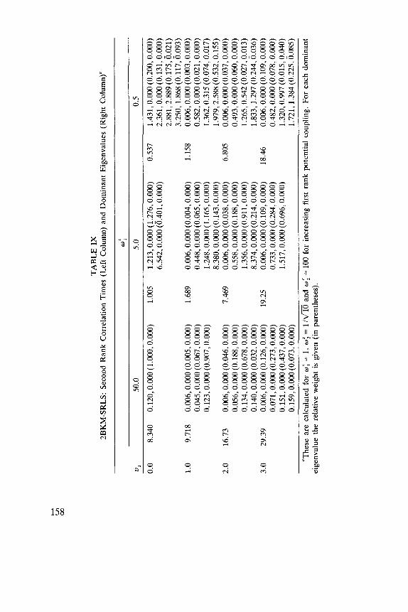
TA
BL
E I
X
2BK
M-S
RL
S: S
econ
d R
ank
Cor
rela
tion
Tim
es (
Lef
t C
olum
n) a
nd D
omin
ant
Eig
enva
lues
(R
ight
Col
umn)
"
w;
u,
50.0
5.0
0.5
0.0
8.340
0.120.0.000(1.000,0.000)
1.0
9.718
0.006,0.000(0.005,0.000)
0.045,O.OOO (0.067,O.OOO)
0.123,O.OOO (0.907,O.OOO)
2.0
16.73
O.OO6,O.OOO (0.046,O.OOO)
0.056,O.OOO (0.188,O.OOO)
0.134,O.OOO (0.678,O.OOO)
0.140,O.OOO (0.032,O.OOO)
3.0
29.39
0.006,0.000(0.126,0.000)
0.071,O.OOO (0.273,O.OOO)
0.151,O.OOO (0.437,O.OOO)
0.159,O.OOO (0.073,O.OOO)
1.005
1.213,0.000(1.276,0.000)
6.542.0.000 (0.401.0.000)
1.689
0.006,0.000(0.004,0.000)
0.448,O.OOO (0.065,O.OOO)
1.248,O.OOO (1.165,O.OOO)
8.380,O.OOO (0.143,O.OOO)
7.469
0.006,O.OOO (0.038,O.OOO)
0.558.0.000 (0.188,O.OOO)
1.356,O.OOO (0.911,O.OOO)
8.374,O.OOO (0.214.0.000)
19.25
0.006,0.000(0.109,0.000)
0.733,O.OOO (0.284,O.OOO)
1.517.0.000 (0.696,O.OOO)
0.537
1.431,0.0OO(0.200,0.000)
2.361,0.000(0.131,0.000)
2.881,2.889 (0.175,0.021)
3,250,1368 (0.117,0.093)
1.158
0.OO6,0.000(0.003,0.000)
0.582,O.OOO (0.021,O.OOO)
1.362,0.315 (0.074,0.017)
1.979,2.588 (0.532,0.155)
6.805
0.006,O.OOO (0.037,O.OOO)
0.493,O.OOO (0.060,O.OOO)
1.265,0.542 (0.027,0.013)
1.833, 1.297 (0.244,0.036)
18.46
0.006,O.OOO (0.109,O.OOO)
0.482.0.000 (0.078,O.OOO)
1.320,0.997 (0.015,0.040)
1.721,1.384 (0.225.0.085)
"The
se a
re c
alcu
late
d fo
r w
; =
1, w
; =
1/m
and
wi =
100 f
or i
ncre
asin
g fi
rst
rank
pot
enti
al c
oupl
ing.
For
eac
h do
min
ant
eige
nval
ue t
he r
elat
ive
wei
ght
is g
iven
(in
par
enth
eses
).
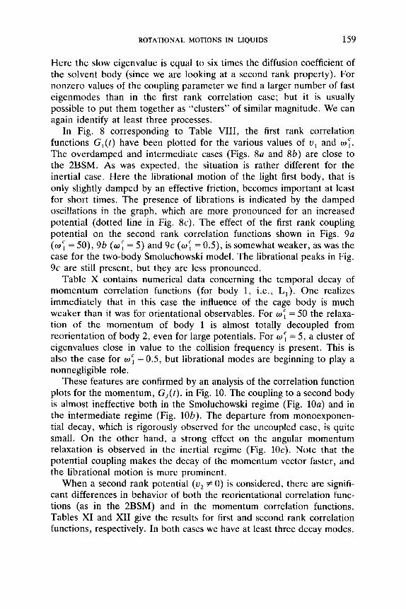
ROTATIONAL MOTIONS IN LIQUIDS 159
Here the slow eigenvalue is equal to six times the diffusion coefficient of the solvent body (since we are looking at a second rank property). For nonzero values of the coupling parameter we find a larger number of fast eigenmodes than in the first rank correlation case; but it is usually possible to put them together as “clusters” of similar magnitude. We can again identify at least three processes.
In Fig. 8 corresponding to Table VIII, the first rank correlation functions G,(t) have been plotted for the various values of u , and 0;. The overdamped and intermediate cases (Figs. 8a and 8b) are close to the 2BSM. As was expected, the situation is rather different for the inertial case. Here the librational motion of the light first body, that is only slightly damped by an effective friction, becomes important at least for short times. The presence of librations is indicated by the damped oscillations in the graph, which are more pronounced for an increased potential (dotted line in Fig. 8c). The effect of the first rank coupling potential on the second rank correlation functions shown in Figs. 9a (uf = 50) , 9b (uf = 5 ) and 9c (ui = O S ) , is somewhat weaker, as was the case for the two-body Smoluchowski model. The librational peaks in Fig. 9c are still present, but they are less pronounced.
Table X contains numerical data concerning the temporal decay of momentum correlation functions (for body 1, i.e., L l ) . One realizes immediately that in this case the influence of the cage body is much weaker than it was for orientational observables. For uf = 50 the relaxa- tion of the momentum of body 1 is almost totally decoupled from reorientation of body 2, even for large potentials. For uT = 5 , a cluster of eigenvalues close in value to the collision frequency is present. This is also the case for uf = 0.5, but librational modes are beginning to play a nonnegligible role.
These features are confirmed by an analysis of the correlation function plots for the momentum, G,(t), in Fig. 10. The coupling to a second body is almost ineffective both in the Smoluchowski regime (Fig. 10a) and in the intermediate regime (Fig. 106). The departure from monoexponen- tial decay, which is rigorously observed for the uncoupled case, is quite small. On the other hand, a strong effect on the angular momentum relaxation is observed in the inertial regime (Fig. 1Oc). Note that the potential coupling makes the decay of the momentum vector faster, and the librational motion is more prominent.
When a second rank potential (u2 # 0) is considered, there are signifi- cant differences in behavior of both the reorientational correlation func- tions (as in the 2BSM) and in the momentum correlation functions. Tables XI and XI1 give the results for first and second rank correlation functions, respectively. In both cases we have at least three decay modes.
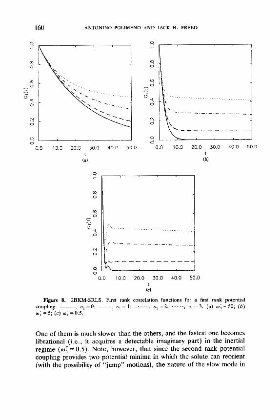
160 ANTONINO POLIMENO AND JACK H. FREED
? ,--
c9 0
x x
n 4 v
0
@! 0
z 0.0 10.0 20.0 30.0 40.0 50.0
I
1
........................ ....................
0.0 10.0 20.0 30.0 40.0 50.0 t
(b)
( . ............................................... . .
, I
0.0 10.0 20.0 30.0 40.0 50.0 t (C)
Figure 8. 2BKM-SRLS. First rank correlation functions for a first rank potential coupling: - u = O . .... u = I . ..... u = 2 . ....., ~ , = 3 . (a ) ~ ; = 5 0 ; ( b )
7 1 9 ? I 1 7 1 1
0: = 5; ( c ) 0; = 0.5.
One of them is much slower than the others, and the fastest one becomes librational (i.e., it acquires a detectable imaginary part) in the inertial regime (of = 0.5). Note, however, that since the second rank potential coupling provides two potential minima in which the solute can reorient (with the possibility of “jump” motions), the nature of the slow mode in

ROTATIONAL MOTIONS IN LIQUIDS 161
n 2 . c v
s x 2 .
0.0 10.0 20.0 30.0 40.0 50.0 t
(a)
. . . . . . . . . . . . . . . . . . . . . . . . . . . . . , . . . . . . . ._ - . _ . _
0.0 10.0
9 -
20.0 30.0 40.0 50.0 t
(b)
- 0.0 10.0 20.0 30.0 40.0 50.0
t (C)
Figure 9. 2BKM-SRLS. Second rank correlation functions for a first rank potential > I u = 2 . 7 . . . .., u , = 3 . (a) w ; = 5 O ; ( b ) coupling: -, u , = o ; _ _ _ _ 3 1 u = 1. 1
w ; = 5; ( c ) w ; = 0.5.
the case of first rank correlation functions is no longer simply the overall relaxation of the solvent body. The situation is very close to the 2BSM for a second rank potential for w i = 50. The relaxation of the momentum vector L, is so fast that we are virtually in a completely diffusive regime.
In the intermediate regime ( w T = 5) inertial effects become more

TA
BL
E X
2BKM-SRLS: M
omen
tum
Cor
rela
tion
Tim
es (
Lef
t C
olum
n) a
nd D
omin
ant
Eig
enva
lues
(R
ight
Col
umn)
"
w:
u1
50.0
5.0
0.5
0.0
0.020
50.0
0,0.
000(
1.00
0,0.
000)
0.200
5.00,0.000(1.000,0.000)
2.000
0.50
0,0.
000(
1.00
0,0.
000)
1.0
0.020
50.0
1,0.
000(
1.00
0,0.
000)
0.197
4.882,0.000(0.413,0.000) 1.425
0.499,0.000(0.267,0.000)
5.200,0.000 (0.355,0.000)
0.684,0.431 (0.240,0.162)
5.661,0.000 (0.263,0.000)
1.231,0.000 (0.304,O.OOO)
7.096.0.000 (0.023,0.000)
2.430,0.000 (0.090,0.000)
2.0
0.02
0 50.02,0.000(0.999,0.000)
0.189
4.656,0.000(0.094,0.000) 0.904
0.50
0,0.
000(
0.14
2,0.
000)
5.151,0.000 (0.226,0.000)
0.733.0.918 (0.099.0.085)
5.794,0.000 (0.697,O.OOO)
1.033,0.000 (0.090,0.000)
7.563,0.000 (0.402,O.OOO)
1.730,0.025 (0.920,0.153)
3.0
0.020
50.02.0.000 (0.998,0.000)
0.181
4.423,0.000 (0.024,O.OOO)
0.654
0.500,0.000 (0.054,0.000)
5.915,0.000 (0.817,0.000)
0.741.1.324 (0.026,0.041)
8.160.0.627 (0.092,0.942)
0.978,0.000 (0.072,0.000)
1.415,0.000(0.305,0.000)
"The
se a
re c
alcu
late
d fo
r w
; =
1,
w; =
1 /a
and
w; =
100 f
or i
ncre
asin
g fir
st r
ank
pote
ntia
l co
uplin
g. F
or e
ach
dom
inan
t ei
genv
alue
the
rel
ativ
e w
eigh
t is
giv
en (
in p
aren
thes
es).
ROTATIONAL MOTIONS IN LIQUIDS 163
0.0 1.0 2.0 3.0 4.0 5.0 t (a)
I 0.0 1.0 2.0 3.0 4.0 5.0
t (6)
7
c9 0
'4 0 ,-. u v
6 ". 0
N 0
8 0.0 1.0 2.0 3.0 4.0 5.0
t (C)
Figure 10. 2BKM-SRLS. Momentum correlation functions for a first rank potential coupling: - OJ; = 5; ( c ) O J ; = 0.5.
u = 0. - _ _ _ , I " = 1. 7 -.-.- , u1 = 2 ; ....., U , =3 . (a ) w ; = 5 0 ; ( b ) 3 1 7
important. The relaxation of the momentum L, is coupled to the slow mode corresponding to the jump motion. The net result is a decreased effective friction acting on this mode, so that the dominant frequency of first rank correlation functions is increased. This effect is also present when the collision frequency is further reduced (OJ; = 0.5). Note however
TABLE X
I 2BKM-SRLS: Firs
t R
ank
Cor
rela
tion
Tim
es (
Lef
t C
olum
n),
Dom
inan
t E
igen
valu
es (
Rig
ht C
olum
n)"
and
Som
e C
orre
spon
ding
Eig
enve
ctor
sb
CI
Q\
P
w:
U,
50.0
5.0
0.5
0.0
25.00
0.040,O.OOO (1 .O
OO, 0
.000
)
1.0
31.27
0.023,0.000(0.559,0.000)
0.058,O.OOO (0.435,O.OOO)
2.0
59.73
0.012.0.000 (0.659,O.OOO)
0.084,O.OOO (0.319.0.000)
0.245,O.OOO (0.015.0.000)
3.0
126.8
0.006,0.000(0.753,0.000)
0.121,O.OOO (0.208,O.OOO)
0.267,O.OOO (0.035,O.OOO)
2.646
0.377,O.OOO ( 1.000.0.000)
3.485
0.198.0.000 (0.502,O.OOO)
0.597,O.OOO (0.576,O.OOO)
2.314,O.OOO (0.017,O.OOO)
7.843
0.085.0.000 (0.630,O.OOO)
0.895,O.OOO (0.405,O.OOO)
2.724,O.OOO (0.220,O.OOO)
1.283,O.OOO (0.208,O.OOO)
2.961, 1.181 (0.026,0.176)
21.55
0.034,O.OO (0.733,O.OOO)
1.036
0.702,O.OOO (0.438,O.OOO)
1.145,1.822 (0.276,0.349)
1.848
0.270,0.000(0.417,0.000)
1.064,1.720 (0.388,0.215)
1.200,2.270 (0.027,0.049)
6.43 1
0.094,O.OOO (0.596.0.000)
0.956,1.944 (0.463,0.012)
1.349,1.795,(0.118,0.139)
+ fa
ster
mod
es
21.02
0.034,O.OOO (0.722,O.OOO)""
Eig
enva
lue lla
lc,l
l n1
n2
i,
12
i
Jl
J2
J
0.267
0
0
0 0
0 1
0
1 0.003
1 0
0 0
0
1 0
1 0.526
0
0
0 0
0
1 2
1 0.007
1 0
0 0
0 1
2
1 0.069
0
0
0
0
0
3
2
1 0.102
0
0 0
0 0
3
4
1 0.003
0
0
0
0
0
5 4
1 0.002
0
0 1
0
1 1
0
1
"The
se a
re c
alcu
late
d w
; =
1,
wi =
1 /a
and
0;
= 100 f
or i
ncre
asin
g se
cond
ran
k po
tent
ial
coup
ling.
For
eac
h do
min
ant
bJT
is c
onst
ant
and
equa
l to
1.
eige
nval
ue t
he r
elat
ive
wei
ght
is g
iven
(in
par
enth
eses
).
TABLE X
I1
2BKM-SRLS: Se
cond
Ran
k C
orre
lati
on T
imes
(L
eft
Col
umn)
and
Dom
inan
t E
igen
valu
es (
Rig
ht C
olum
n)”
w:
v2
50.0
5.0
0.5
0.0
8.340
0.12
0,0.
000(
1.00
0,0.
000)
1.005
1.213,0.000(1.276.0.000) 0.537
1.431,0.000(0.200,0.000)
6.542,0.000 (0.401,0.000)
2.361,0.000 (0.131,0.000)
2.881,2.889 (0.17S,6.021)
3.250, 1.868 (0.117,0.093)
1.0
16.69
0.006.0.000(0.053,0.000) 9.138
0.006.0.000(0.049.0.000)
8.618
0.006,0.000 (O.OS0,0.000)
0.116,O.OOO (0
.655
.0.0
00)
1.104.0.000 (0.300.0.000)
0.693,O.MKI (0.094,O.OOO)
0.132.0.000 (0.123.0.000)
1.251,0.000 (0.557,0.000)
1.707, 1.047, (0.177.0.051)
0.147,0.000 (0
.160
,0.0
00)
1.438,0.000 (0.353,O.OOO)
1.976,1.887,
(0.264,0.036)
2.0
41.38
0.00
6,0.
000(
0.21
1,0.
000)
32.92
0.006,0.000(0.195,0.000) 32.67
0.006,0.000(0.192,0.000)
0.126,0.000 (0.399,O.OOO)
1.123,0.000 (0.207.0.000)
0.489,O.OOO (0.111,O.OOO)
0.140,0.000 (0.237,0.000)
1.582,0.000 (0.753,0.000)
1.269,2.377 (0.064.0.211)
0.177,0.000 (0
.120
,0.0
00)
1.778,O.OOO (0.082.0.000)
3.0
70.07
0.006,0.000(0.394,0.OOO)
56.5
2 0.006,0.000(0.370,0.000)
61.34
0.006,0.000(0.366,0.000)
0.148,0.000 (0.100,0.000)
1.260.0.000 (0.108,0.000)
0.428.0.000 (0
.080
,0.0
00)
0.163,0.000 (0.387.0.000)
1.993,O.OOo (0.125,0.000)
1.147,2.772 (0.019,0.448)
0.217,0.000 (0.109,O.OOO)
2.576,O.OOO (0.732,O.OOO)
“Th
ese
are
calc
ulat
ed fo
r w
; =
1,
w’,
= l
/fi an
d w
; =
100
for
incr
easi
ng se
cond
ran
k po
tent
ial c
oupl
ing.
For
eac
h do
min
ant
eige
nval
ue t
he r
elat
ive
wei
ght
is g
iven
(in
par
enth
eses
).
166 ANTONINO POLIMENO AND JACK H . FREED
that the rate of change of the eigenvalue with decreasing w ; is slowed down, and it is negligible when the potential is high; that is, for u2 = 1 the eigenvalue goes from 0.023 (wT=50) , to 0.198 ( w i = 5 ) and 0.270 ( w ; = 0.5); for u2 = 2 it goes from 0.012 to 0.085 and 0.094; finally for u2 = 3 it goes from 0.006 to 0.034 and 0.034, that is, it remains unchanged when the collision frequency is reduced by a factor of ten. This may be due to an incipient Kramers turnover effect. It is possible that for a larger potential, the jump eigenmode would invert its dependence versus wf by starting to increase when the collision frequency is decreased.
Nothing of this sort is observed for second rank correlation functions, since the dominant slow mode is simply a FRD of the solvent body. In both first and second rank correlation functions one notes that librational modes are slightly more important when the potential coupling is second rank than they were for a first rank potential coupling. This may be due to the increased curvature of the potential near the minima.
The complex nature of the slow mode responsible for the long-time behavior of first rank correlation functions for a first rank interaction potential is illustrated by the composition of the eigenvector correspond- ing to the slow mode l l a in Table XI, for u2 = 3 and wf = 0.5. Note that n , , n, , jl , j , describe the magnitudes and the orientations of the momen- tum vectors L, and L,; j is referred to the orientation of L, + L,, J , and J2 are related to the orientations of the two bodies, and the total orienta- tional angular operator defines the quantum number J ; finally J , , which is not included in this table, is the total angular momentum quantum number, and it is always equal to 1 for first rank orientational and momentum correlation functions, and to 2 for second rank correlation functions. In Fig. 11 we show the first rank correlation functions for different collision frequencies of body 1. The second rank correlation function decays are plotted in Fig. 12. The librational motions in the wells are more important than they were in the first rank potential case (since there is now a more accentuated curvature of the potential wells).
In Table XI11 we show momentum correlation functions. One finds that there are increased librational effects from the second rank potential. Compare for instance the case of u2 = 3 and w i = 5 with the correspond- ing entry in Table X (u l = 3 and w i = 5 ) . In the present case the librational mode is dominant and the simple decay mode has a weight only half that of the case in Table X, for which most of the decay is by a nonlibrational mode. The interpretation of the dominant modes is com- plicated when the potential is large and the regime of motion of the solute body is inertial. In Table XI11 some of the eigenvectors corresponding to the dominant eigenvalues for u2 = 3 and w i = 0.5 are shown. It is not possible to isolate a single component having a coefficient larger than 0.5
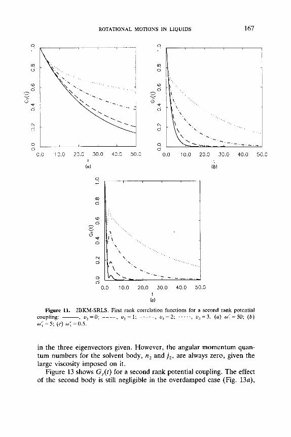
ROTATIONAL MOTIONS IN LIQUIDS 167
8 0.0 10.0 20.0 30.0 40.0 50.0
t (a)
0.0 10.0 20.0 30.0 40.0 50.0 t
(b)
"..
. z
0.0 10.0 20.0 30.0 40.0 50.0 t
(C)
Figure 11. 2BKM-SRLS. First rank correlation functions for a second rank potential coupling: - - 2 u = 0. 3 ---- r 2 . u = 1. -.-.-, u2 = 2; . . . . ., u2 = 3. ( a ) OJ; = 50; ( b ) O J ; = 5; ( c ) OJ: = 0.5.
in the three eigenvectors given. However, the angular momentum quan- tum numbers for the solvent body, n2 and j 2 , are always zero, given the large viscosity imposed on i t .
Figure 13 shows G,(t) for a second rank potential coupling. The effect of the second body is still negligible in the overdamped case (Fig. 13a),
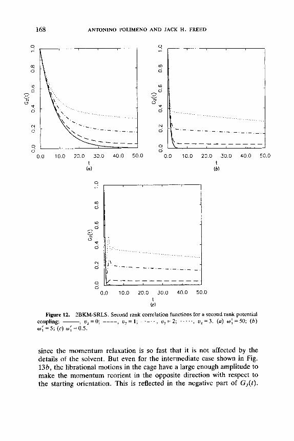
168 ANTONINO POLIMENO AND JACK H. FREED
. . . . . . . . . . . . . _ . ........... ........................
I ' . - - - . - . - I
0.0 10.0 20.0 30.0 40.0 50.0 t
(C)
Figure 12. 2BKM-SRLS. Second rank correlation functions €or a second rank potential coupling: - u = 0. _--- u x 1. -.-.- , u 2 = 2 ; ..... , u2 = 3. (a) OJ; = 50; ( b ) r 2 , 7 2 9
~f = 5; (c) m f = 0.5.
since the momentum relaxation is so fast that it is not affected by the details of the solvent. But even for the intermediate case shown in Fig. 136, the librational motions in the cage have a large enough amplitude to make the momentum reorient in the opposite direction with respect to the starting orientation. This is reflected in the negative part of G,(t) .
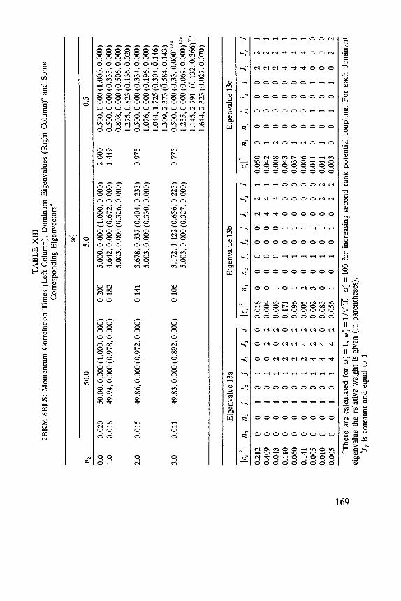
TA
BL
E X
I11
2BK
M-S
RL
S: M
omen
tum
Cor
rela
tion
Tim
es (
Lef
t C
olum
n), D
omin
ant
Eig
enva
lues
(R
ight
Col
umn)
” an
d So
me
Cor
resp
ondi
ng E
igen
vect
orsb
v2
50.0
5.0
0.5
0.0
0.020
50.00,0.000(1.000,0.000) 0.200
5.000,0.000(1.000,0.000) 2.000
0.500,0.000(1.000,0.000)
1.0
0.018
49.94.0.000(0.978,0.000) 0.182
4.642,0.000(0.672,0.000)
1.449
0.500,0.000(0.333,0.000)
5.003,O.OOO (0.326,O.OOO)
0.80
8,0.
000 (0.506,O.OOO)
1.275,0.823 (0.136.0.020)
2.0
0.015
49.86,0.000(0.972,0.000) 0.141
3.678,0.537(0.404,0.233) 0.975
0.500,0.000(0.334,0.000)
5.003,0.000 (0.330,O.OOO)
1.076,O.OOO (0.196,O.OOO)
1.044,1.725 (0.304,6.146)
1.309,2.373 (6.584,0.143)
3.0
0.011
49.83.0.000(0.892,0.000) 0.106
3.172,1.122(0.656,0.223) 0.775
0.500,0.000(0.33,0.000)’1”
5.003,O.OOO (0.327,O.OOO)
1.235,O.OOO (0.069,0.00O)~~~
1.145,2.791,
(6,132,0.366)”‘
1.644.2.323 (0.027.0.070)
Eig
enva
lue 13a
Eig
enva
lue 13b
Eig
enva
lue 13c
k,12
n1
n2
i, j,
i J
, J,
J
14’
n,
n,
i, i2
i J
, J~
J
Ic,1
2 n,
n,
i,
i, i
J,
J2
J
0.212
0
0 1
0 1
0 0
0
0.018
0
0 0 0
0 2 2 10.050
0 0
0 0
0 2 2
1 0.4090 0 1010220.0040 0
00
04
41
0.
04
21
0
00
02
21
0.0430
0 1012020.0051 0
00
04
41
0.
00
82
00
00
22
1
0.110
0 0 1
0 1
2 2 00.171
0 0 1
0 1
0 0
00.043 0 0
0 0
0 4 4
1 0.0600 0
10
12
22
0.
09
61
01
01
00
00
.0
37
1 0
00
04
41
0.1410 0
10
12
42
0.
00
52
01
01
00
00
.0
06
2 0
00
04
41
0.005
0
0 1
0 1
4 2 20.002 3 0 1
0 1
0 0
00.011
0 0 1
0 1
0 0
0 0.010
0 0 1
0 1
4 4 00.083 0 0 1
0 1
0 2 20.011 1
0 1
0 1
0 0
0 0.005
0
0 1
0 1
4 4 20.056 1
0 1
0 1
0 2 20.003 0
0 1
0 1
0 2 2
“The
se a
re c
alcu
late
d fo
r w
; =
1,
w; =
l/m,
0; =
100 f
or i
ncre
asin
g se
cond
ran
k po
tent
ial
coup
ling.
For
eac
h do
min
ant
’.IT
is c
onst
ant
and
equa
l to
1.
c.r m
\o
eige
nval
ue t
he r
elat
ive
wei
ght
is g
iven
(in
par
enth
eses
).
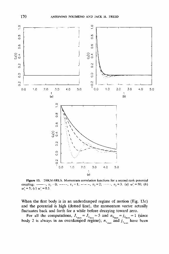
170 ANTONINO POLIMENO AND JACK H . FREED
I
0.0 1.0 2.0 3.0 4.0 5.0 t (a)
I 0.0 1.0 2.0 3.0 4.0 5.0
0 c
2
z ,--. z t 3 0
"! 0
8 2 I 0.0 1.0 2.0 3.0 4.0 5.0
t (C)
Figure 13. 2BKM-SRLS. Momentum correlation functions for a second rank potential coupling: __ 7 2 , u = o . _--- , 2 , u = 1' - .-.- , u2 = 2 ; . . .. . , u2 = 3. (a) w ; = 50; ( b ) w ; = 5 ; ( c ) w f =0.5.
When the first body is in an underdamped regime of motion (Fig. 13c) and the potential is high (dotted line), the momentum vector actually fluctuates back and forth for a while before decaying toward zero.
For all the computations, J,,,, = JZnlax - 5 and n2,,, = j2, , , , = 1 (since body 2 is always in an overdamped regime); n,,,, and j , , , , have been
-

ROTATIONAL MOTIONS IN LIQUIDS 171
both set equal to 1 for wf = 50, to 2 for wf = 5 and to 5 for wf = 0.5 and the number of Lanczos steps was between 100 and 500. Note that the largest matrices treated (for w ; = 0.5 and u2 = 3) had dimensions of order los!
5. Two-Body Fokker-Planck-Kramers Model: FT Case
The last model considered in this work is a variation on the previous inertial two-body approach. Instead of allowing a direct source of cou- pling between the two bodies via a simple interaction potential, we now introduce a frictional coupling between them. This is the residual effect after the elimination as fast variables, of a stochastic field vector and its conjugate linear momentum (see Section 1I.G). The model is an inertial counterpart of the 3BSM described above, provided the “third body” is relaxing fast enough that only its averaged effect on the torques acting on the two principal bodies is left. This case is equivalent to similar models with “fluctuating torques” (FT) features (cf. Stillman and Freed [33]).
Both the SRLS and the FT inertial models were discussed in the context of the Hubbard-Einstein relation, that is, the relation between the momentum correlation time T, and the rotational correlation time (second rank) T~ for a stochastic Brownian rotator [39]. It was shown that both models can cause a substantial departure from the simple expression predicted by a one-body Fokker-Planck-Kramers equation:
I 7,r2 = -
6k,T (2.93)
In the IT case, it was found that the additional friction due to the fast field has a different effect on the rotational versus momentum relaxation, such that, whereas T~ still behaves in a “normal” fashion (i.e., it is roughly proportional to the total friction, from both the solvent terms and the field terms), T, is not much influenced by the friction generated by the fast field. These comments apply to the case in which the sources of friction are large, so that the system is always in a diffusional regime.
These matters are described in more detail in the last set of calcula- tions included in the present work. We have considered a fixed “core” friction (from the unspecified fast solvent modes) and fixed dimensions for the second body: w i = l/m, wS = 100, with w ; = 1 for the first body (so it is ten times smaller than body 2). We have investigated two cases: w i = 50 and wf = 5. The additional source of coupling, according to Section II.F, is specified by the frictional parameters w l , w2. To further simplify the analysis we have kept w2 = l o w , , and we have varied w, from 0 to 400.
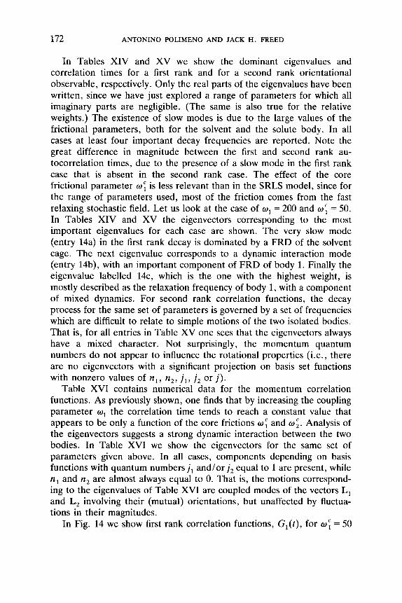
172 ANTONINO POLIMENO A N D JACK H . FREED
In Tables XIV and XV we show the dominant eigenvalues and correlation times for a first rank and for a second rank orientational observable, respectively. Only the real parts of the eigenvalues have been written, since we have just explored a range of parameters for which all imaginary parts are negligible. (The same is also true for the relative weights.) The existence of slow modes is due to the large values of the frictional parameters, both for the solvent and the solute body. In all cases at least four important decay frequencies are reported. Note the great difference in magnitude between the first and second rank au- tocorrelation times, due to the presence of a slow mode in the first rank case that is absent in the second rank case. The effect of the core frictional parameter w i is less relevant than in the SRLS model, since for the range of parameters used, most of the friction comes from the fast relaxing stochastic field. Let us look at the case of w1 = 200 and w i = 50. In Tables XIV and XV the eigenvectors corresponding to the most important eigenvalues for each case are shown. The very slow mode (entry 14a) in the first rank decay is dominated by a FRD of the solvent cage. The next eigenvalue corresponds to a dynamic interaction mode (entry 14b), with an important component of FRD of body 1. Finally the eigenvalue labelled 14c, which is the one with the highest weight, is mostly described as the relaxation frequency of body 1, with a component of mixed dynamics. For second rank correlation functions, the decay process for the same set of parameters is governed by a set of frequencies which are difficult to relate to simple motions of the two isolated bodies. That is, for all entries in Table XV one sees that the eigenvectors always have a mixed character. Not surprisingly, the momentum quantum numbers do not appear to influence the rotational properties (i.e., there are no eigenvectors with a significant projection on basis set functions with nonzero values of n,, n,, j , , j , or j ) .
Table XVI contains numerical data for the momentum correlation functions. As previously shown, one finds that by increasing the coupling parameter w1 the correlation time tends to reach a constant value that appears to be only a function of the core frictions w i and w ; . Analysis of the eigenvectors suggests a strong dynamic interaction between the two bodies. In Table XVI we show the eigenvectors for the same set of parameters given above. In all cases, components depending on basis functions with quantum numbers j , and/or j , equal to 1 are present, while n , and n, are almost always equal to 0. That is, the motions correspond- ing to the eigenvalues of Table XVI are coupled modes of the vectors L, and L, involving their (mutual) orientations, but unaffected by fluctua- tions in their magnitudes.
In Fig. 14 we show first rank correlation functions, G , ( t ) , for wf = 50
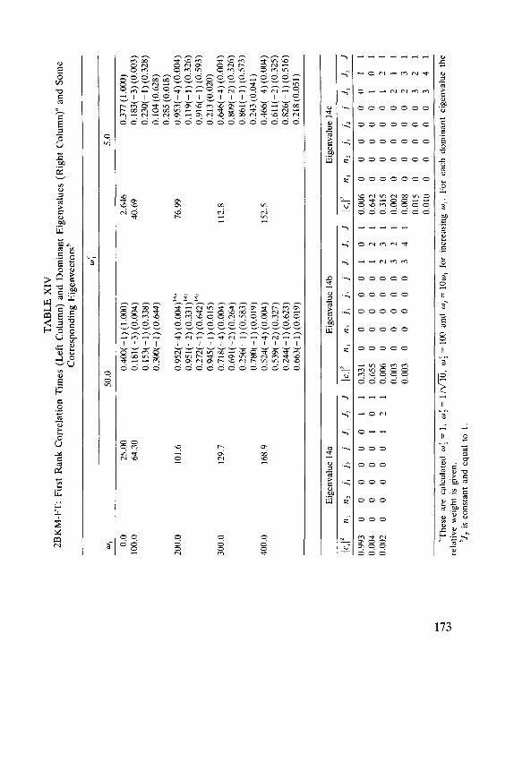
L 4
w
TA
BL
E X
IV
2BK
M-F
T:
Fir
st R
ank
Cor
rela
tion
Tim
es (
Lef
t C
olu
mn
) an
d D
omin
ant
Eig
enva
lues
(R
igh
t C
olum
n)"
and
Som
e C
orre
spon
ding
Eig
enve
ctor
sb
w1
50.0
5.
0
200.
0
300.
0
400.
0
101.
6
129.
7
168.
9
0.0
25.0
0 0.
400(
-1)
(1.0
00)
100.
0 64
.30
0.18
1(-3
) (0
.004
) 0.
153(
-1)
(0.3
38)
0.30
0(-1
) (0.644)
0.95
2(-4
) (0
.004
)'"
0.95
1(-2
) (0
.331
)lab
0.
272(
-1)
(0.6
42)1
5'
0.94
5( - 1
) (0.
015)
0.
718(
-4)
(0.0
04)
n.69
1(-2
) (0
.264
) 0.
256(
-1)
(0.5
83)
0.78
0(-1
) (0
.019
) 0.
524(
-4)
(0.0
04)
0.53
9(-2
) (0
.327
) 0.
244(
-1)
(0.6
23)
0.66
3(-1
) (0
.019
)
76.9
9
112.
8
152.
5
0.37
7 (1
.000
) 2.
646
40.6
9 n
.m-
3)
(0.
003)
0.
230(
- 1
) (0.
328)
0.
104
(0.6
28)
0.28
5 (0
.018
) 0.
953(
- 4)
(0.
004)
0.
119(
- 1)
(0.3
26)
0.91
6(-1
) (0
.593
)
0.64
6(-4
) (0
.004
) 0.
809(
-2)
(0.3
26)
0.86
1(-1
) (0
.573
)
0.46
6(-4
) (0
.004
) 0.
611(
-2)
(0.3
25)
0.82
6(-1
) (0
.516
)
0.21
3 (0
.020
)
0.24
3 (0
.041
)
0.21
8 (0
.051
)
Eig
enva
lue
14a
Eig
enva
lue
14b
lc,I
2 n
I nz
i,
i2
i
J,
Jz
J lc
,I2
n, nz
i,
iz
i J
, J
2
J
0.99
3 0
0 0
0 0
0 1
1 0.
331
0 0
0 0
0 I
0 1
0.00
4 0
0 0
0 0
1 0
1 0.
655
0 0
0 0
0 1
2 1
0.0
02
0
00
00
1 2
10
.0
06
0
00
00
23
1
0.00
3 0
0 0
0 0
3 2
1 0.
003
0 0
0 0
0 3
4 1
Eig
enva
lue
14c
IC,r
0.00
6 0.
642
0.31
5 0.
002
0.00
8 0.
015
0.01
0
n,
n2
i,
i2
i
J,
J2
J
00
00
00
11
0
00
00
10
1
00
00
01
21
0
00
00
21
1
00
00
02
31
0
00
00
32
1
00
00
03
41
"The
se a
re c
alcu
late
d w
; =
1,
0;
= 1
/m, w
; =
100
and
w2
= l
ow,
for
incr
easi
ng w
,. F
or e
ach
dom
inan
t ei
genv
alue
the
'J,
is co
nsta
nt a
nd e
qual
to
1.
rela
tive
wei
ght
is gi
ven.
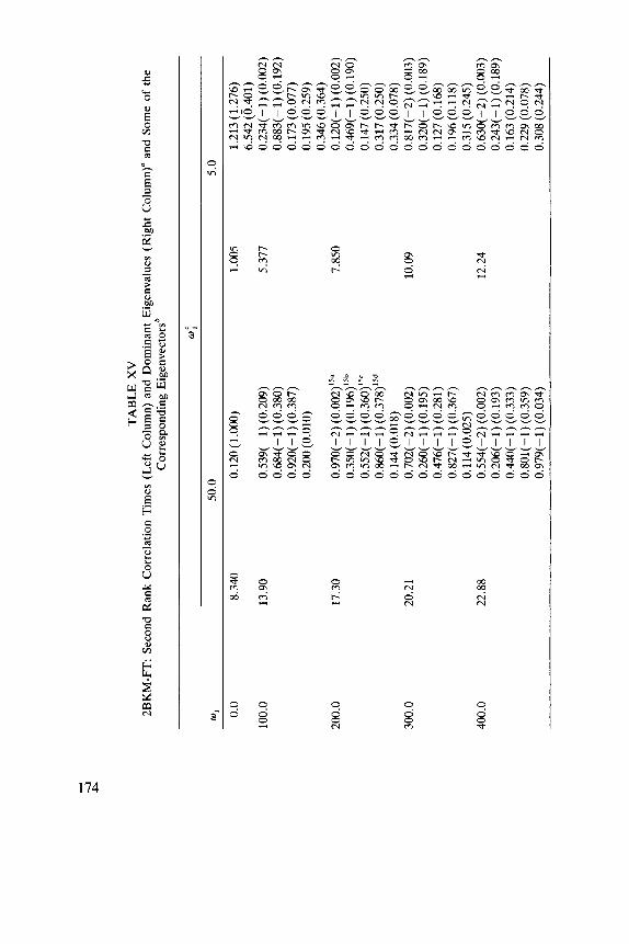
L 4
P
TA
BL
E X
V
2BK
M-F
T:
Seco
nd R
ank
Cor
rela
tion
Tim
es (
Lef
t C
olum
n) a
nd D
omin
ant
Eig
enva
lues
(R
ight
Col
umn)
" an
d S
ome
of t
he
Cor
resp
ondi
ng E
igen
vect
ors*
w;
01
50
.0
5.0
0.0
100.
0
200.
0
300.
0
400.
0
8.34
0
13.9
0
17.3
0
20.2
1
22.8
8
0.12
0 (1
.000
)
0.53
9(-1
) (0
.209
) 0.
684(
- 1
) (0.
380)
0.
920(
-1)
(0.3
87)
0.20
0 (0
.010
)
0.97
0(-2
) (0
.002
)1sa
0.
350(
- 1)
(0.1
96)l
sb
0.55
2(-1
) (0
.360
)1s'
0.
860(
- 1
) ( 0.
378)
lsd
0.70
2(-2
) (0
.002
) 0.
260-
1)
(0.1
95)
0.47
6(-1
) (0
.281
) 0.
827(
-1)
(0.3
67)
0.55
4( -2
) (0
.002
) 0.
206(
-1)
(0.1
93)
0.44
0(-1
) (0
.333
) 0.
801(
-1)
(0.3
59)
0.97
9(-1
) (0
.034
)
0.14
4 (0
.018
)
0.11
4 (0
.025
)
1.00
5
5.37
7
7.85
0
10.0
9
12.2
4
1.21
3 (1
.276
) 6.
542
(0.4
01)
0.23
4(-
1) (0
.002
) 0.
883(
-1)
(0.1
92)
0.17
3 (0
.077
) 0.
195
(0.2
59)
0.34
6 (0
.364
) 0.
120(
-1)
(0.0
02)
0.46
9(-1
) (0
.190
) 0.
147
(0.2
50)
0.31
7 (0
.250
) 0.
334
(0.0
78)
0.81
7(-2
) (0
.003
) 0.
320(
- 1)
(0.1
89)
0.12
7 (0
.168
) 0.
196
(0.1
18)
0.31
5 (0
.245
) 0.
630(
-2)
(0.0
03)
0.24
3(-1
) (0
.189
) 0.
163
(0.2
14)
0.22
9 (0
.078
) 0.
308
(0.2
44)
Eig
enva
lue
1Sa
I4
n
l nz
il
i, i
Jl
J2
J
0.39
5 0
0 0
0 0
1 1
2 0.
583
0 0
0 0
0 1
3 2
0.00
2 0
0 0
0 0
2 0
2 0.
011
0 0
0 0
0 2
4 2
0.00
2 0
0 0
0 0
3 1
2 0.
002
0 0
0 0
0 3
3 2
0.00
2 0
0 0
0 0
3 5
2
Eig
enva
lue
15b
lc,l’
n1
n2
i, i2
i
J,
J,
J
0.00
3 0
0 0
0 0
1
3 2
0.19
7 0
0 0
0 0
2 0
2 0.
277
0 0
0 0
0 2
2 2
0.46
4 0
0 0
0 0
2 4
2 0.
001
0 0
0 0
0 3
3 2
0.03
6 0
0 0
0 0
3 5
2 0.
011
0 0
0 0
0 4
2 2
0.01
0 0
0 0
0 0
4 4
2
Eig
enva
lue
1%
Eig
enva
lue
1Sd
0.00
9 0
0 0
00
1 3
2
0.36
0 0
0 0
0 0
2 0
2 0.
127
0 0
0 0
0 2
2 2
0.35
8 0
0 0
0 0
2 4
2 0.
112
0 0
0 0
0 3
5 2
0.02
9 0
0 0
0 0
4 2
2 0.
002
0 0
0 0
0 4
4 2
0.00
2 0.
002
0.37
7 0.
522
0.02
2 0.
001
0.02
9 0.
006
n,
n2
i,
i2
i J,
J
, J
00
00
01
12
0
00
00
13
2
00
00
02
02
0
00
00
22
2
00
00
02
42
0
00
00
31
2
00
00
03
32
0
00
00
35
2
“The
se a
re c
alcu
late
d fo
r O
; =
1,
O: =
l/
m,
w: =
100
, w
2 =
100
, fo
r in
crea
sing
w,.
For
eac
h do
min
ant
eige
nval
ue t
he
hJT
is co
nsta
nt a
nd e
qual
to
2.
rela
tive
wei
ght
is g
iven
(in
par
enth
eses
).
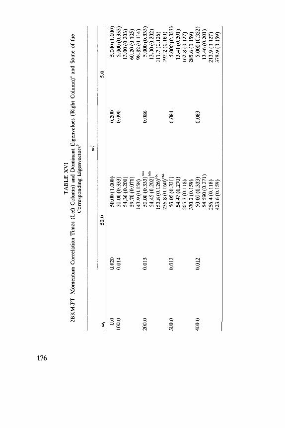
TA
BL
E X
VI
ZB
KM
-FT
: M
omen
tum
Cor
rela
tion
Tim
es (
Lef
t C
olum
n) a
nd D
omin
ant
Eig
enva
lues
(R
ight
Col
umn)
" an
d So
me
of t
he
Cor
resp
ondi
ng E
igen
vect
orsb
w.
50.0
5.
0
0.0
0.02
0 50
.00
(1.0
00)
0.20
0 5.
000
(1.0
00)
100.
0 0.
014
50.0
0 (0
.333
) 0.
090
5.00
0 (0
.333
) 54
,36
(0.2
01)
13.0
0 (0
.203
) 59
.70
(0.0
71)
60.2
0 (0
.105
) 14
3.9
(0.1
58)
98.8
2 (0
.114
)
54.4
5 (0
.202
)16h
13
.30
(0.2
02)
200.
0 0.
013
50.0
0 (0
.333
)16"
0.
086
5.00
0 (0
.333
)
153.
8 (0
.126
)16'
11
1.7
(0.1
26)
192.
2 (0
.160
) 23
6.8
(0.1
60)1
6d
300.
0 0.
012
50.0
0 (0
.331
) 0.
084
5.00
0 (0
.333
) 54
.47
(0.2
70)
13.4
1 (0
.201
) 20
5.3
(0.1
18)
162.
8 (0
.127
) 33
0.2
(0.1
59)
285.
6 (0
.159
) 40
0.0
0.01
2 50
.00
(0.3
33)
0.08
3 5.
000
(0.3
32)
54.5
90 (0
.271
) 13
.46
(0.2
01)
256.
4 (0
.118
) 21
3.9
(0.1
27)
423.
6 (0
.159
) 37
8.9
(0.1
59)
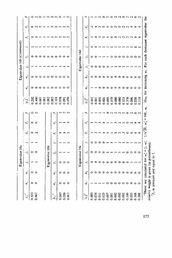
'1 01 lenba pue IU
EISU
OJ sI "f,
aq, an
pu
aZ!a iueu!m
op qx
a J
OJ
.'m
%u!seaim
! lo3 '"01 =
im '001 = :m '0
1
I = :m '1 =
:m 103 paielnqer, ale asaq
l,
Z P
P I
0 I
0 0
OI
I'O
Z
P P
I0
I0
0 88E'O
0
P P
I0
I0
0 8
E0
.0
0
P P
I0
I0
0 891'0
Z P
Z
I0
I0
0 9
00
'0
Z
Z 0
I0
I0
0 ESO'O
Z Z
Z I
0 I
0 0
9L
E'O
O
0 0
I0
I0
0 901'0
0 z
z I
0 I
0 0
EE
I'
OZ
I
E I
I0
0 0
ZOO'O z
o z
TO
I0
0 0
8O
.O
Z
1 E
I T
O 0
0 ZOO'O
Z Z
0 T
O T
O 0
08
0'
0Z
E
I I
I0
0 0
ZOO'O 0
0 0
I0
I0
0 6
51
'0
Z
I I
I I
0 0
0 100'0
z s
s I
I0
0 0
EO
O'
OO
I
I I
I0
0 0
LOO'O 0
s s
II
0 0
0 100'0
I P
P 0
0 0
0 I
SZO'O z
E E
11
0 0
0 I
00
'0
1
E E
0 0
0 0
11
10
'0
I
PP
OO
OO
I 100'0
I z
z 0
0 0
0 I
PEO'O 1
zz
00
00
I ZOO'O
I I
I 0
0 0
0 I
€00'0
'(sasaqlualed U!) U
aA
@ Sf l@
aM
JA
!IElaJ
b
2
f
Zf '[
f y
'I zu
1u J
3(
f Zf
'f I
Z! zu
'u 2)'3)
p91 anIeAua%
g 391 an[E
AU
J%g
z z
z I
0 I
0 0
OLO'O I
Z Z
I 0
I 0
0 160'0
0 Z
Z I
0 I
0 0
8E0'0
z 0
z I
0 I
0 0
101'0 Z
E 1
10
1 0
OE
OO
'O
z
I I
I 0
I 0
0 ZOO'O
I I
I I
0 I
0 0
100'0 0
I I
I 0
I 0
0 100'0
z z
0 I
0 I
0 0
OOP'O 0
0 0
1 0
I 0
0 ZOZ'O
[
if 'I
/ il
'I ;u
'14
;1!31
(panu
puo3) q91 a
np
ua
%!q
z E
I I
1 0
0 0
LIO'O Z
I I
I I
0 0
0 9ZO
'O
I I
I I
I 0
0 0
EPO'O
Z 0
Z I
0 I
0 0
L99'0
0 0
0 I
0 I
0 0
EEE'O
f if
'f I
iI
'I iu
'u
;I
13
1
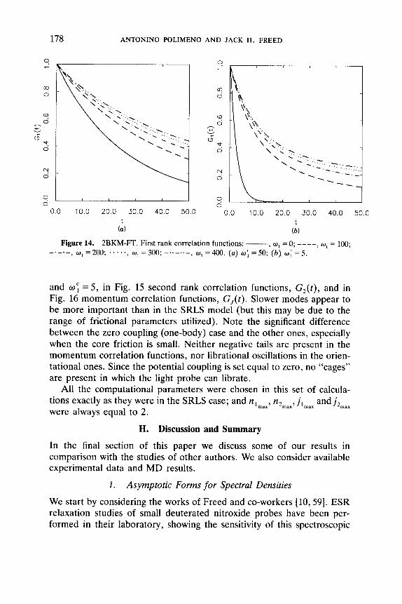
178 ANTONINO POLIMENO AND JACK H . FREED
0
0.0 10.0 20.0 30.0 40.0 50.0 t (a)
I
0.0 10.0 20.0 30.0 40.0 50.0 1
(b )
Figure 14. 2BKM-FT. First rank correlation functions: - 3 1 w = 0. 3 ---- , w, = 100; -._.- , ~ , = 2 0 0 ; ....., ~ , = 3 0 0 ; - . . - . . - , ~ , = 4 0 0 . (a ) ~ ; = 5 0 ; ( b ) ~ ; = 5 .
and wT = 5 , in Fig. 15 second rank correlation functions, G2(t), and in Fig. 16 momentum correlation functions, G,(t). Slower modes appear to be more important than in the SRLS model (but this may be due to the range of frictional parameters utilized). Note the significant difference between the zero coupling (one-body) case and the other ones, especially when the core friction is small. Neither negative tails are present in the momentum correlation functions, nor librational oscillations in the orien- tational ones. Since the potential coupling is set equal to zero, no “cages” are present in which the light probe can librate.
All the computational parameters were chosen in this set of calcula- tions exactly as they were in the SRLS case; and n,,,,, n2,,,, jl,,, and j2,,, were always equal to 2.
H. Discussion and Summary
In the final section of this paper we discuss some of our results in comparison with the studies of other authors. We also consider available experimental data and MD results.
1 . Asymptotic Forms for Spectral Densities
We start by considering the works of Freed and co-workers [lo, 591. ESR relaxation studies of small deuterated nitroxide probes have been per- formed in their laboratory, showing the sensitivity of this spectroscopic
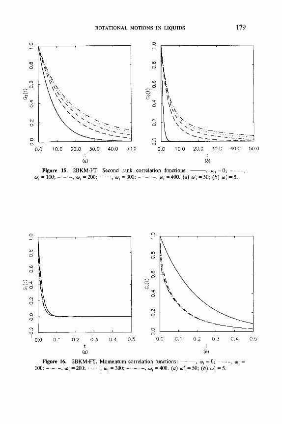
9 c
8
x x 2
x
?-. * 4 s
ROTATIONAL MOTIONS IN LIQUIDS 179
0.0 10.0 20.0 30.0 40.0 50.0 0.0 10.0 20.0 30.0 40.0 50.0 t t (a) (b )
Figure 15. 2BKM-FT. Second rank correlation functions: - 3 1 w =0. 3 ----, 0 = 100. -.-.-, w1 = 200; . . . . . , w1 = 300; -..-..-, w, = 400. (a) w ; 4 0 ; ( b ) w: = 5.
'4 0
N 0
9
?
0
0
8
'4 0 - c v
G ": 0
N 0
x ' 0.0 0.1 0.2 0.3 0.4 0.5 0.0 0.1 0.2 0.3 0.4 0.5 t t (a) (b)
Figure 16. 2BKM-IT. Momentum correlation functions: - , I , w =0 . ---- , 0, = 100; _._.- , 0,=200; ....., wl=300; -..-..-, wl=400. (a ) w ; = 5 0 ; (b ) w ; = 5 .
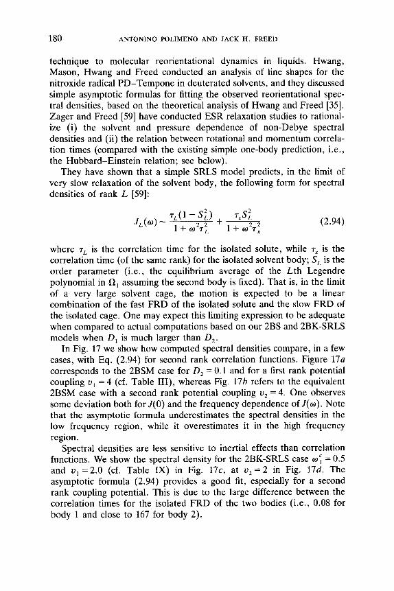
180 ANTONINO POLIMENO AND JACK H. FREED
technique to molecular reorientational dynamics in liquids. Hwang, Mason, Hwang and Freed conducted an analysis of line shapes for the nitroxide radical PD-Tempone in deuterated solvents, and they discussed simple asymptotic formulas for fitting the observed reorientational spec- tral densities, based on the theoretical analysis of Hwang and Freed [35]. Zager and Freed [59] have conducted ESR relaxation studies to rational- ize (i) the solvent and pressure dependence of non-Debye spectral densities and (ii) the relation between rotational and momentum correla- tion times (compared with the existing simple one-body prediction, i.e., the Hubbard-Einstein relation; see below).
They have shown that a simple SRLS model predicts, in the limit of very slow relaxation of the solvent body, the following form for spectral densities of rank L [59]:
(2.94)
where T~ is the correlation time for the isolated solute, while T~ is the correlation time (of the same rank) for the isolated solvent body; S , is the order parameter (i.e., the equilibrium average of the Lth Legendre polynomial in R, assuming the second body is fixed). That is, in the limit of a very large solvent cage, the motion is expected to be a linear combination of the fast FRD of the isolated solute and the slow FRD of the isolated cage. One may expect this limiting expression to be adequate when compared to actual computations based on our 2BS and 2BK-SRLS models when D, is much larger than D,.
In Fig. 17 we show how computed spectral densities compare, in a few cases, with Eq. (2.94) for second rank correlation functions. Figure 17a corresponds to the 2BSM case for D, = 0.1 and for a first rank potential coupling u, = 4 (cf. Table 111), whereas Fig. 176 refers to the equivalent 2BSM case with a second rank potential coupling u, = 4. One observes some deviation both for J(0) and the frequency dependence of J(w) . Note that the asymptotic formula underestimates the spectral densities in the low frequency region, while it overestimates it in the high frequency region.
Spectral densities are less sensitive to inertial effects than correlation functions. We show the spectral density for the 2BK-SRLS case oT = 0.5 and u , = 2.0 (cf. Table IX) in Fig. 17c, at u, = 2 in Fig. 17d. The asymptotic formula (2.94) provides a good fit, especially for a second rank coupling potential. This is due to the large difference between the correlation times for the isolated FRD of the two bodies (i.e., 0.08 for body 1 and close to 167 for body 2).
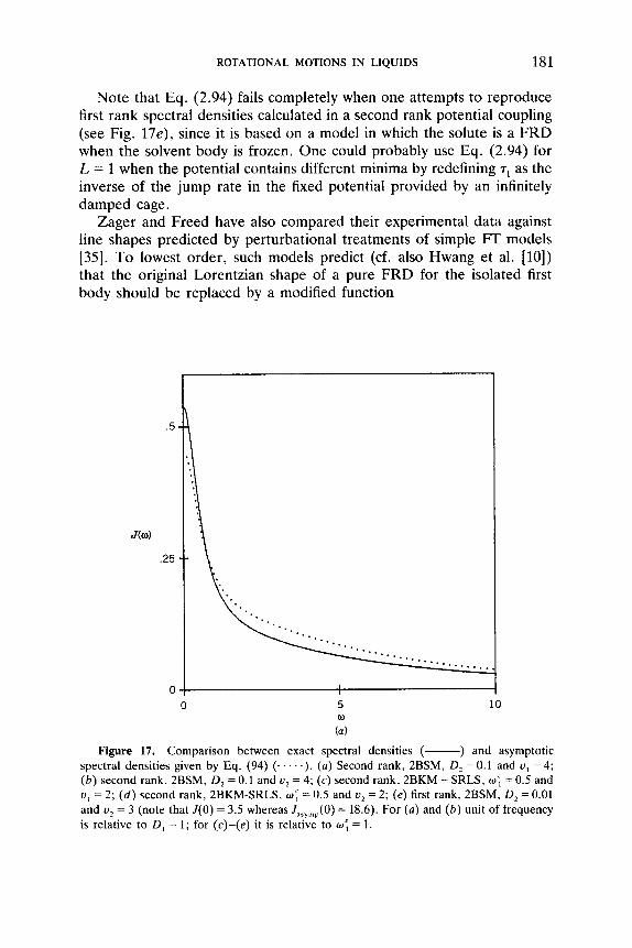
ROTATIONAL MOTIONS IN LIQUIDS 181
Note that Eq. (2.94) fails completely when one attempts to reproduce first rank spectral densities calculated in a second rank potential coupling (see Fig. 17e), since it is based on a model in which the solute is a FRD when the solvent body is frozen. One could probably use Eq. (2.94) for L = 1 when the potential contains different minima by redefining T, as the inverse of the jump rate in the fixed potential provided by an infinitely damped cage.
Zager and Freed have also compared their experimental data against line shapes predicted by perturbational treatments of simple FT models [35]. To lowest order, such models predict (cf. also Hwang et al. [lo]) that the original Lorentzian shape of a pure FRD for the isolated first body should be replaced by a modified function
0 10
Figure 17. Comparison between exact spectral densities (-) and asymptotic spectral densities given by Eq. (94) (. . .. .). ( a ) Second rank, 2BSM, D2 = 0.1 and u , = 4; (b) second rank, 2BSM, D, = 0.1 and u2 = 4; (c) second rank, 2BKM - SRLS, w ; = 0.5 and u , = 2; (d) second rank, 2BKM-SRLS. w ; = 0.5 and u, = 2; (e) first rank, 2BSM, D, = 0.01 and u, = 3 (note that J ( 0 ) = 3.5 whereas Ja,>,,,p(0) = 18.6). For ( a ) and (b) unit of frequency is relative to D, = 1; for (c ) - (e ) i t is relative to 0; = 1 .
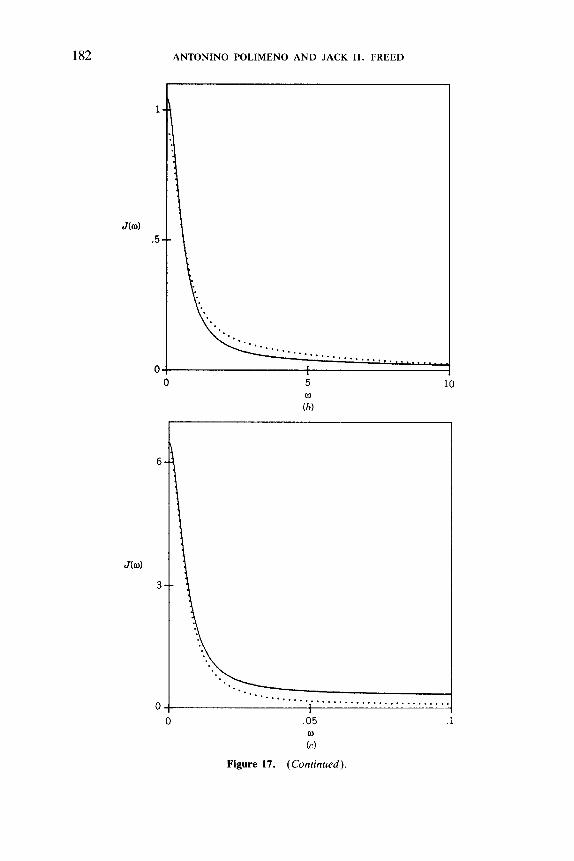
182
1
0
6
0 0
ANTONINO POLIMENO AND JACK H . FREED
5 10
.05
( C )
0
Figure 17. (Continued).
.1
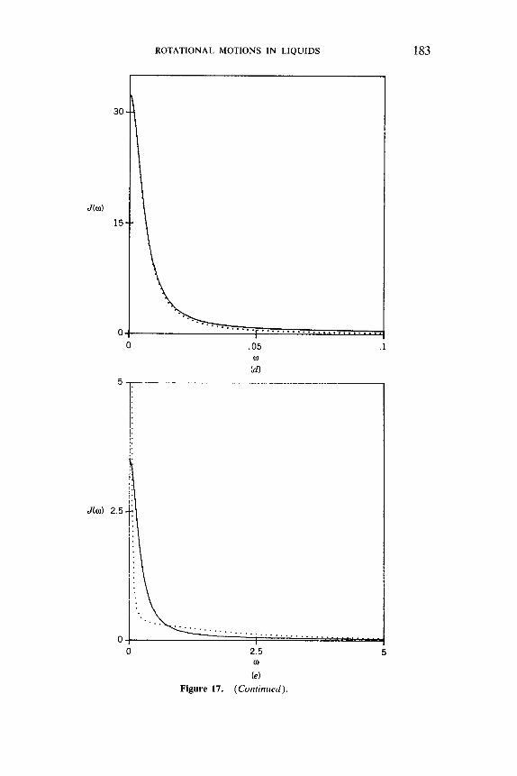
30
0.
5
0
ROTATIONAL MOTIONS IN LIQUIDS 183
.05 .1
(d) w
2.5
(e)
w
Figure 17. (Corztiizired)
5
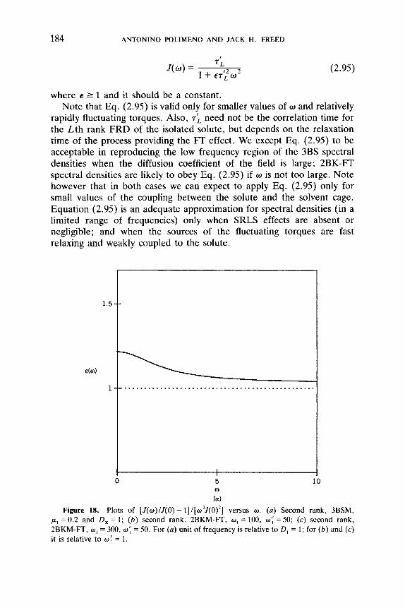
184 ANTONINO POLIMENO AND JACK H . FREED
(2.95)
where E 2 1 and it should be a constant. Note that Eq. (2.95) is valid only for smaller values of w and relatively
rapidly fluctuating torques. Also, T; need not be the correlation time for the Lth rank FRD of the isolated solute, but depends on the relaxation time of the process providing the FT effect. We except Eq. (2.95) to be acceptable in reproducing the low frequency region of the 3BS spectral densities when the diffusion coefficient of the field is large; 2BK-FT spectral densities are likely to obey Eq. (2.95) if w is not too large. Note however that in both cases we can expect to apply Eq. (2.95) only for small values of the coupling between the solute and the solvent cage. Equation (2.95) is an adequate approximation for spectral densities (in a limited range of frequencies) only when SRLS effects are absent or negligible; and when the sources of the fluctuating torques are fast relaxing and weakly coupled to the solute.
0 5
(a) w
Figure 18. Plots of [ J (w) / J (O) - l]/[w’J(O)’] versus w. (a ) Second rank, 3BSM, y, = 0.2 and D, = 1 ; ( b ) second rank, 2BKM-FT, w, = 100, u: = 50; (c) second rank, 2BKM-FT, w, = 300, w ; = 50. For (a ) unit of frequency is relative to D, = 1; for ( b ) and (c) it is relative to w : = 1.
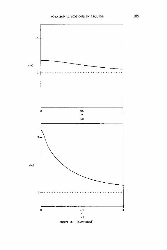
ROTATIONAL MOTIONS IN LIQUIDS
--
185
-- ................................................
I I
1.5
&(a)
1
0 .05 .1
(b) a
...............................................
0 .05
(C)
w
Figure 18. (Continued).
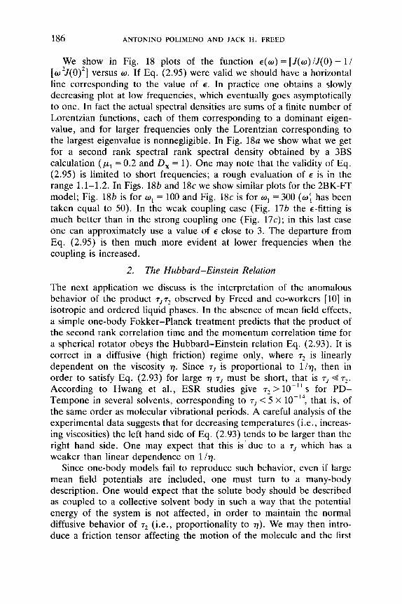
186 ANTONINO POLIMENO AND JACK H . FREED
We show in Fig. 18 plots of the function E ( W ) = [ J ( w ) / J ( O ) - 1/ [w2J(0 )2 ] versus w. If Eq. (2.95) were valid we should have a horizontal line corresponding to the value of E . In practice one obtains a slowly decreasing plot at low frequencies, which eventually goes asymptotically to one. In fact the actual spectral densities are sums of a finite number of Lorentzian functions, each of them corresponding to a dominant eigen- value, and for larger frequencies only the Lorentzian corresponding to the largest eigenvalue is nonnegligible. In Fig. 18a we show what we get for a second rank spectral rank spectral density obtained by a 3BS calculation ( p1 = 0.2 and D, = 1). One may note that the validity of Eq. (2.95) is limited to short frequencies; a rough evaluation of E is in the range 1.1-1.2. In Figs. 18b and 18c we show similar plots for the 2BK-FT model; Fig. 18b is for w1 = 100 and Fig. 18c is for w1 = 300 ( w ; has been taken equal to 50). In the weak coupling case (Fig. 176 the €-fitting is much better than in the strong coupling one (Fig. 17c); in this last case one can approximately use a value of E close to 3 . The departure from Eq. (2.95) is then much more evident at lower frequencies when the coupling is increased.
2. The Hubbard-Einstein Relation
The next application we discuss is the interpretation of the anomalous behavior of the product T,T? observed by Freed and co-workers [lo] in isotropic and ordered liquid phases. In the absence of mean field effects, a simple one-body Fokker-Planck treatment predicts that the product of the second rank correlation time and the momentum correlation time for a spherical rotator obeys the Hubbard-Einstein relation Eq. (2.93). It is correct in a diffusive (high friction) regime only, where is linearly dependent on the viscosity 77. Since T~ is proportional to 1/77, then in order to satisfy Eq. (2.93) for large 77 T/ must be short, that is T/ -e 7:. According to Hwang et al., ESR studies give T?> lo-" s for PD- Tempone in several solvents, corresponding to T/ < 5 x 10-l4, that is, of the same order as molecular vibrational periods. A careful analysis of the experimental data suggests that for decreasing temperatures (i.e., increas- ing viscosities) the left hand side of Eq. (2.93) tends to be larger than the right hand side. One may expect that this is 'due to a T~ which has a weaker than linear dependence on 1/77.
Since one-body models fail to reproduce such behavior, even if large mean field potentials are included, one must turn to a many-body description. One would expect that the solute body should be described as coupled to a collective solvent body in such a way that the potential energy of the system is not affected, in order to maintain the normal diffusive behavior of (i.e., proportionality to 77). We may then intro- duce a friction tensor affecting the motion of the molecule and the first
ROTATIONAL MOTIONS IN LIQUIDS 187
solvation sphere, such that the variation of T~ is “damped” when the friction is large.
We choose to describe our coupled system by using the 2BK-FT model, without any torque contribution (zero potential). The collisional matrix is provided by Eq. (2.72). The diagonal terms wf and 0 4 are kept constant, whereas the coupling terms w1 and w2 are changed, for a fixed ratio of the moments of inertia of the two bodies. In this way one expects to model the effect of a fast fluctuating torque (directly related, in our approximation, to the fast relaxing reaction field) which provides the largest friction, and which rapidly varies with temperature and/or pres- sure. The rest of the solvent provides merely a constant damping that is supposed to be less affected by a change in temperature and pressure, at least in the range of parameters considered in the few experiments that are available.
An analysis of this kind has been made in our recent paper [39], for a solvent cage ten times larger than the solute, a streaming frequency for the solute equal to lo1* and an overall friction, parametrized by w1 ranging from lo1* to 10ls s-l, using the same numerical techniques described in this chapter. In that study, it has been confirmed that for such pure FT models, the correlation time behaves approximately in a “diffusive” way, that is, it increases with the increase of the total friction acting on the solute (proportional to w1 + w ; ) .
An entirely different behavior is observed for the angular momentum correlation time. The coupling terms in the collisional matrix, causing the mutual friction between body 1 and body 2 are much more important. The momentum correlation function is largely dominated by the eigen- values of the collisional matrix. This means that for large coupling ( w l S = - u f ) the dominant eigenmode for the momentum tends to be proportional to the smallest eigenvalue of the collisional matrix, which is practically equal to w f , the “core” friction. Thus the particular structure of the friction tensor of a 2BKM-FT provides a way of interpreting the slow change with temperature of 7,. Our present, more extensive study confirms this analysis (cf. Table XVI).
The 2BKM-SRLS model can also cause a substantial departure from the Hubbard-Einstein relation [39]. This is because T~ = ~ ~ ( 1 - S:) + T,S: [cf. Eq. (2.94)], so rR increases with increased potential coupling and with increase in size of the solvent cage. However, momentum relaxation is dominated by eigenmodes that are primarily the FRD of the isolated solute (cf. Tables X and XIII).
3. Molecular Dynamics Simulations
Molecular dynamics (MD) simulations are an important way of providing insight into motions in liquid phases. In recent years, such simulations
188 ANTONINO POLIMENO AND JACK H . FREED
have been extensively employed to study the properties of model fluids consisting of interacting molecules and to obtain reorientational and angular velocity correlation functions. Stochastic models can be thought of as complementary theoretical tools to MD, since they may provide (i) general models to interpret results from MD observations, which may be regarded as ideal experiments, and (ii) information at long-times, where for computational reasons MD simulations are not feasible.
The complex rotational behavior of interacting molecules in the liquid state has been studied by a number of authors using MD methods. In particular we consider here the work of Lynden-Bell and co-workers [60-621 on the reorientational relaxation of tetrahedral molecules [60] and cylindrical top molecules 1611. In [60], both rotational and angular velocity correlation functions were computed for a system of 32 molecules of CX, (i.e., tetrahedral objects resembling substituted methanes, like CBr, or C(CH,),) subjected to periodic boundary conditions and inter- acting via a simple Lennard-Jones potential, at different temperatures. They observe substantial departures of both G,,*(f) and G,(t) from predictions based on simple theoretical models, such as small-step diffu- sion or J-diffusion [58]. Although we have not attempted to quantitatively reproduce their results with our mesoscopic models, we have found a close resemblance to our 2BK-SRLS calculations. Compare for instance our Fig. 13 with their Fig. 1 in [60].
In particular they consider a set of simulations for a system of CX, molecules at three different temperatures (“hot”, “intermediate” and COO^") which bears a close resemblance to our computations made in the presence of a second rank interaction potential. Their “hot” case corre- sponds to our low potential coupling cases, whereas their “cool” simula- tion is related to our high potential results: that is, a decrease in temperature corresponds in our rescaled coordinates to an increase in the potential coupling. One may note that the presence of a negative tail, assigned by Lynden-Bell to librational motion of the observed molecule in an instantaneous cage, causes the momentum correlation functions to behave differently in the “cool” state with respect to the purely diffusive decay observed for the “hot” state. This behavior is very similar to our 2BKM-SRLS case for ~f = 5 and u2 = 3 (cf. Fig. 13b).
4. Impulsive Stimulated Scattering Experiments
In the last few years Nelson and co-workers [63-6.51 have presented a new approach to light scattering spectroscopy, named impulsive stimulated light scattering (ISS), which seems to be able to detect one particle rotational correlation functions. In ISS, one induces coherent vibrational motion by irradiating the sample with two femtosecond laser pulses, and
ROTATIONAL MOTIONS IN LIQUIDS 189
then observes a light scattering intensity signal decaying in time. The ISS spectrum is resolved in the time domain and can be directly related to second rank rotational correlation function G,(t) [65]. Thus ISS is one of the few spectroscopic techniques which appears to give, at least in some cases, direct information on single-molecule rotational dynamics, together with nuclear magnetic resonance (NMR), electron spin resonance (ESR) and neutron scattering.
In particular, Nelson and co-workers have collected a set of ex- perimental data concerning the reorientational dynamic of CS, both in temperature-dependent [64] and pressure-dependent [65] ISS experi- ments. In both cases they observed “weakly oscillatory responses” in the signal either for low temperature regimes or for high pressure regimes. These have been identified as librational motions of the probe molecule in the transient local potential minima inside the instantaneous cages formed by its neighbors.
Comparable behavior has been observed by Fayer et al. in a series of subpicosecond transient grating optical Kerr effect measurements on the reorientation of byphenyl molecules in neat biphenyl and n-heptane solutions [66,67]. They have shown that on the ultrafast timescale ( t < 2 ps) the dynamics of the probe is controlled by librational motions having an inertial character, although diffusive reorientational relaxation of the whole molecule and internal torsional motions can also have a role.
The analysis of local librations in terms of the few existing tractable theoretical models (e.g., IOM) have shown that although a qualitative agreement can be reached with experiments, the interpretation of the short time dynamic behavior remains an open problem. We think that our methodology could help to clarify some aspects of the experimental observations.
5. Summary
A careful analysis has been performed on several stochastic models for rotational relaxation of rigid molecules in complex liquids. These include two-body rotational diffusion in the overdamped (Smoluchowski) regime (2BSM), as well as a related three-body model (3BSM). Inertial effects have been considered in two other models which are two-body Fokker- Planck-Kramers models in the full phase space of rotational coordinates and momenta (2BKM). In one, the two bodies interact via an orienta- tion-dependent interaction potential, and this leads to a “slowly relaxing local structure” (SRLS) description. In the other there is an orientation- dependent frictional coupling, derivable from other faster solvent modes, which leads to a “fluctuating torque” (FT) description. The computation- al challenge of solving multidimensional Fokker-Planck equations has

190 ANTONINO POLIMENO AND JACK H. FREED
been dealt with by (i) constructing efficient sets of basis functions utilizing angular momentum coupling techniques; (ii) utilizing the complex sym- metric Lanczos algorithm to obtain the orientational and angular momen- tum correlation functions. These correlation functions have been ana- lyzed in terms of the dominant “normal modes” with their associated decay constants.
For the 2BSM, the effect of a large solvent cage yields biexponential behavior with significantly different decay rates. While this behavior may be approximated by modes related to the original free rotational diffusion (FRD) of each body in the absence of coupling, these modes become more influence by “dynamic interactions” for increased interaction poten- tial and/or more nearly equal rotational diffusion coefficients of the two bodies. It has been shown that first rank versus second rank potentials lead to significantly different behaviors, especially for first rank correla- tion functions (i.e., G,( t ) ) . In this case, a second rank potential leads to an apparent “strong collision effect”, that is, a two-body small-step diffusion which exhibits features typical of a one-body strong collision model. Previous simpler SRLS models are inconsistent with this effect. Also, one finds that second rank correlation functions [ G2(r)] have somewhat complex behavior with several decay modes, and with in- creased importance of dynamic interactions. The 3BSM leads to more pronounced departure from single exponential decay. When inertial effects are included via the 2BKM-SRLS case, there are still fast modes for orientational relaxation with purely real decay constants (correspond- ing to solute modes that are largely diffusional), but now there are solute modes with complex decay constants corresponding to librational motion. For G , ( t ) with second rank potentials, the coupling of the angular momentum to the jump motion leads to unusual behavior that may be an incipient Kramers turnover effect. Angular momentum correlation func- tions [GL(r)] have been found to be much less influenced by the solvent cage than are orientational observables, except for the importance of librational motion in nearly inertial regimes with such motion being enhanced by second rank potentials. These librational modes have been found to have a complex character. In the 2BKM-FT case there are no librational motions. Instead one observes that the FT has little effect on the solute angular momentum correlation time despite the fact that it leads to strong dynamic coupling of the two angular momenta. However, the FT makes an important frictional contribution to the orientational relaxation, such that there is a significant breakdown of the Hubbard- Einstein relation.
These results have been compared with previous studies to show: ( i ) a simple SRLS model used in ESR is reasonable in the asymptotic limit of a
ROTATIONAL MOTIONS IN LIQUIDS 191
very slow solvent cage except when a “strong collision effect” (cf. above) is important; (ii) the E correction to a Debye spectral density, used in ESR to account for FT, only has a limited validity for low frequencies and relatively rapid but weak torques; (iii) the G,(t) with a second rank potential resembles molecular dynamics simulations on spherical tops in showing librational motion in an instantaneous cage; (iv) new light scattering results for G2(t) appear to have features accountable with the present models.
APPENDIX A: CUMULANT PROJECTION PROCEDURE
In this appendix we review briefly the TTOC (total time ordered cumul- ant) procedure applied to a general linear time evolution operator. The same technique was used by Stillman and Freed [33]; for other details see Yoon et al. [28] and Hwang and Freed [35], and references quoted therein. Also we show how to apply the TTOC procedure for projecting out a subset of fast momenta, from a phase space of coordinates and momenta.
1 . General Algorithm
We start by considering a system described by the set of generalized coordinates (and momenta) (qs, qf )
The time evolution operator is supposed to be given by
We now introduce a biorthonormal complete set of functions defined in the q, subspace
(nln’) = 8(n - n’) (A.3)
where n is a collective index for the set of quantum numbers labeling these functions. Note that (1) In) and (nI could be the set of eigenfunc- tions of r, and its adjoint, respectively, or at this stage, of any other operator acting on the phase space spanned by qf ; (2) in general we do not suppose here that n is a collection of integers, that is, we can consider a continuum of quantum numbers. The function 10) is supposed to be unique and to fulfill the following properties:
192 ANTONINO POLIMENO AND JACK H . FREED
f,lo) = 0
(elf;= 0
that is, 10) is the unique eigenfunction of zero eigenvalue of f; (while this may be not necessarily true for n # 0, according to the previous remark). Note that here we are always dealings with symmetrized operators: for example, if the subsystem defined by q, tends to the equilibrium dis- tribution P,,(q,) for t+ +w then (0) = Pi: = (01. Although not neces- sary from a mathematical point of view, in all the physical applications we have considered, the following equation holds:
Following [33] closely, we now take the time evolution equation for the reduced probability density in just q, as the average over qf obtained by computing the "expectation value" with respect to 10); that is
aP(qs7 f , = -(OlfP(q,, q,, [)lo) at
After Laplace transformation we easily recover the following exact multidimensional equivalent of the result shown in [33]:
h,, 4 = (OKs + f)-'lo)P(q,, 0) (A.8)
where the resolvent (Ol(s + f)-'lO) can be evaluated according to [28,35] as
(OI(s + f)-'lo) = (s + fs - G)-' ('4.9)
and G is defined as
+m
G = c (-)k+'(OIFi",[(s + f, + f,)-'(l - lo>(ol)f,,*lkl0~ *
k = O (A. 10)
If we may assume that the In) are the eigenfunctions of f,, then
ffld = E"l4 (A . l l )
(,If;= (nlE,* (A.12)
ROTATIONAL MOTIONS IN LIQUIDS 193
Then G can be further expanded in + m
G = EJ- n, . . . ~ n j ( O l ~ i n t ~ n l ) ( n l l ( s + ps + Enl)-1pintln2) . . j = l
+ p s + E n ~ - " ~ n t I O ) (A.13)
where 9' n; is a restricted sum (or integral) over all possible ni # 0. If we consider the first order correction only (in the approximation %- IFs\), and we restrict our analysis to low frequencies (s - 0) we obtain
(A.14)
as the first perturbation correction to Fs. 2. Elimination of Some Momenta from a MFPKE
We apply the technique reviewed in the previous section to a MFPKE defined for a set of general coordinates (x, , x2) and their conjugate momenta (p l , p2). The system is divided into two subsystems interacting via a general potential function V and a friction matrix wc
(A.15)
oc is a symmetric definite positive ( N , + N 2 ) X ( N , + N 2 ) dimensional matrix, and it depends on x l , x2. We want to obtain a reduced equation after eliminating all momenta p2. That is, according to the previous section we are considering q, = (x, , p l , x2) and q, = p2. The initial MFPK operator is written as the sum of
Fs = s:,;fi, - R&$; + s;o;s; (A.16)
F,= s;,;s, (A.17)
(A. 18) Fint = s;o;fi, - a,+,;s, + q w r r s , + s;,q where the vector operators R,,, and s,,, are defined as
(A.19)
(A.20)

194 ANTONINO POLIMENO AND JACK H . FREED
For instance, this is the compact form for the symmetrized time evolution MFPK operator for two Brownian particles (or rotators; see below) coupled via a potential V and a frictional (collisional) matrix 0'. Al- though both the terms acting on the momentum space and the positional space are written, for the sake of simplicity, as formal raising and lowering operators, actually only the properties of the $: operators will be used in the following. Note that we have not specified the nature of the gradient operators in xmr so they could be a set of rotational coordinates (in this case we should include a precession-like term in pint; but we shall see in the next section that the presence of the precession operator is irrelevant). We define In) as the direct product of the eigenfunctions of S2iS, i
A + A _
In) = I.JI.2). . . I.,,) (A.21)
s;.s,l.;) = (A.22)
Then n is a collection of integers and the set of functions is orthonormal [52] (i.e., we can neglect the integral symbol in Eq. (A.9)); 5; are the raising and lowering operators with respect to the ith momentum in p2; 10) is the Boltzmann distribution on the momenta p2. However, we cannot apply Eq. (A.13) directly, because 0 5 is not diagonal. We then utilize Eq. (A.9) under the assumption that r, - 1041 is the dominant term (i.e., p2 relaxes very fast relative to the remaining coordinates). Then for low frequencies
(A.23)
where we have used Eq. (A.6) twice. Given that In) is a complete set of basis functions in the subspace p2, we then rewrite Eq. (A.23) in the form
(A.24)
When pint acts on lo), it generates only single excited states, for example, 10. . . 1 . . . O ) . If we call Ilj) the singly excited function in the j th position, it is easy to rewrite the previous expression for G in the form
(A.25)
the summation indexes run from 1 to N7. From the equations
ROTATIONAL MOTIONS IN LIQUIDS 195
it follows that the final reduced operator is given by
where
W; = Of - 000''
f = 000; 0 D, = o;&o;
(A.29)
(A.30)
(A.31)
The new matrix 0 is defined as
(0)$ = (ljlf7' Ilj.) (A.32)
It is now relatively simple to see that 0 is exactly equal to 02'. Let us consider the matrix representation of 4 on In): by inspection, one soon realizes that pf mixes In) and In') if and only if C ni = C n: ; that is, only states equally excited are mixed. The matrix is then partitioned in diagonal blocks; the first block is 1 X 1 (fundamental state); the second one is N2 x N,, mixes only the states C n, = 1, that is the Ilj) functions, and it is given by m;.
3. Precessional Operator
For a rotational system one has to include the precessional operator in the rotational FPK operator, in case a nonspherical top is considered. In terms of the raising and lowering operators SZ defined in the last section (systematically suppressing the subscript 2 since it is understood here that we are dealing entirely only with the subspace p2), we can write the precessional operator as
(A.33)
196 ANTONINO POLIMENO AND JACK H . FREED
where A , , A?, A3 are functions of the streaming frequency matrix elements. Note that
A, + A, + A3 = 0 (A.34)
The crucial point in the ITOC expansion delineated in the last section is that the interaction operator pint acting on 10) generates only single excited states. In this rotational case, we may include the precessional term in rint, and it is easy to see that
A
Pw'VlO,O,O) = -(A, + A, + A,)[(), 0,O) (A.35)
In fact all the factors containing a lowering operator go to zero; and one obtains zero because of Eq. (A.34). This means that it is not necessary to consider the precessional effects in projecting out to lowest order the role of angular momentum.
APPENDIX B: ELIMINATION OF HARMONIC DEGREES OF FREEDOM
Here we show how to implement the ITOC procedure for eliminating in a single step a set of harmonic degrees of freedom together with their conjugate momenta from an initial MFPKE. This technique is applied in Section 1.C to project out the fast field X and its momentum P from the initial three body Fokker-Planck-Kramers equation.
1 . Elimination of One Harmonic Degree of Freedom
We start by considering a one-dimensional example given by the rescaled symmetrized MK evolution operator in the coordinates (xl, x,) and conjugate momenta ( p l , p,),
where the potential V is defined as
1 2 v = VO(Xl) - p ( x l ) x * + -x2 2

ROTATIONAL MOTIONS IN LIQUIDS 197
We introduce the shifted coordinates .f2 = x 2 - p. This canonical trans- formation enables us to obtain a more suitable form for the operator, in which V is decoupled. Neglecting the tilde symbol in the following, we identify q, with (x l , p , ) and qJ with ( x 2 , p2)
and the potential V is now
It is useful now to recall the general properties of the harmonic Kramers operator. We utilize the summary provided by Risken [43]. The raising and lowering operators for the momentum p 2 and the position x2 are given by
where in Eqs. (B7) and (B8) and below in this subsection we suppress the subscript 2 for convenience. The quantities hl,?, solutions of the secular equation A’ - w‘A + wS2 = 0, are calculated. We also define a parameter W
The following operators are then defined:
(B. l l )
198 ANTONINO POLIMENO AND JACK H . FREED
112 A + 1 A - -- ( A : ' , $ - - A, R )
w c1-
C,+ = -1/2 ( - A l S + A:'2k+)
c2- - 1 / 2
1 112 .. t w
-- - 1 ( A ; / 2 $ - + A ; / 2 R - )
w
The following identity is deduced:
f = AIC,+tl- + A2C,+C2-
and eigenfunctions and eigenvalues are easily obtained as
where
and
For the adjoint operator similar equations hold:
where
(B.12)
(B.13)
(B.14)
(B.15)
(B.16)
(B.17)
(B.18)
(B.19)
(B.20)
(B.21)
(B.22)
(B.23)
(B.24)
(B.25)
(B.26)
ROTATIONAL MOTIONS IN LIQUIDS 199
(B.27)
(B.28)
(B.29)
We have so defined a biorthonormal set of functions
b 1 3 n2lnl,, 4) = %,,n;%*,ni (B.30)
We may now use the method of Appendix A for the case of a biorthonor- ma1 discrete set of eigenfunctions. We then have that
From the identities
w ; ap 1 a 0 ax, dP1
t n t l O , 0 ) = - -112 - [-A:” (5 p1 + -) ] L O )
(B.32)
one obtains easily the reduced operator
(B.35) a
aP1 x exp(-p:/2) - exp(p:/4)
where the effective collisional frequency is defined as
(B.36)
Note that both reversible effects (correction to the potential function) and irreversible ones (correction to the initial friction) are obtained.
200 ANTONINO POLIMENO AND JACK H . FREED
2. Elimination of N2 Harmonic Degrees of Freedom
We now generalize this result to a multidimensional case. The initial rescaled and symmetrized operator is split into three parts:
where the averaged potential, on which Rl and R, are defined, is a quadratic function of the vector dipole p,
1 2 V = V , - - p 2
(B.40)
and R:, 8; are the vector equivalents of the previous similar one- dimensional operators. For the sake of simplicity we choose and ~ f , ~ as diagonal and constant. We generalize the previous definitions intro- ducing the matrices 0, A , , 2 and the vector operator i ,+ , 2,- and their adjoints. The eigenfunctions of 4 are the direct product of theeigenfunc- tions of the one-dimensional harmonic Kramers operators. We label each member of the set with the obvious symbol In,, n2) . The zero eigenvalue function is
exp(-p:/4 - x34) (B.41)
and we call fij, O} the first excited state with respect to n, j , etcetera; it is easy to show that
1 ) O , O ) = (0,ol = -
( 2 7 r y 2
(B.42)
(B.43)
(B.44)
ROTATIONAL MOTIONS IN LIQUIDS
6 is now given by
201
(B.45)
and the final reduced operator has the form
I? = q w ; a ; - R,’w$; + i q w f ’ q (B.46)
where the frictional (collisional) matrix is
(B.47)
APPENDIX C: THE REDUCED MATRIX ELEMENTS
We evaluate in this appendix the reduced matrix elements employed in the WE calculations throughout the main text.
1. Reduced Matrix Element of the Torque
To evaluate the reduced matrix element of the torque T, we first rewrite Eq. (2.17) as
T = - i [ (S ,V) , , - (V3,),,1 (C- 1)
where for ( )op what is contained within acts as an operator. From the WE theorem (weak form for noncommuting operators)
The 6 j symbol is readily reduced
The reduced matrix element of 3, is given by Eq. (2.31), while the reduced matrix element of the potential V is
202 ANTONINO POLIMENO AND JACK H. FREED
where the reduced matrix element in the a, subspace only was used (rn = 1 , 2 )
Finally, one obtains
J , J2 J ~ ~ ( ~ l V ) o p l l J I J I J ’ ) = - u,( - ) J i + J 2 [ JJ’J , J J2 J ? ] l i 2
X [ J 1 ( J 1 + 1 ) ( 2 J 1 + 1)]”2
X
{ J~ J 2 } { J 1 J 2 ” } (C.6) J’ J, 1 J ; J ; R
where the definition u, = [R]V, /8r r2 was used. An analogous formula holds for the reduced matrix element of ( V j , ) , ,
[ JJ ‘J ; J2J;]1’2 J1 + J i + I + J ’ ~ J , J , J l / ~ ~ ~ l ~ , , , l l J ; J ~ J ‘ ~ = -u,(-)
X [ J I ( J i + 1 ) ( 2 J I + 1)]1’2
J , R J i ) ( J 2 R J ;
I’ J ; J ; J ; R
x ( o o o 0 0 0 [ I ; J ?}{ J , J , J ’ ]
so that, finally
( J , J , J I I T I I ” J ; J ‘ ) = ~ u , [ J J ’ J , J ; J ~ J ; ] ’ ’ ~ ( J I ) J , R J I ) ( J 2 R
x [ ( - ) J i+J2[J , ( J l + 1)(2J, + l>J”z { J”: ?}
- (-)J,+JG+J+J’ [ J ; ( J ; + 1 ) ( 2 J ; + 1 ) ] l i 2
X { J I J ? } ( J 1 5 2 J ] ] J ’ J I J ; J ; R

ROTATIONAL MOTIONS IN LIQUIDS 203
2. Vector representation of P::
Since PLr is a zero rank tensor, we can simply write Eq. (2 .26) as
since we have already found J = 0 and M = 0. By inspection, one can see that I J , J200) (coupled basis set function) is proportional to 9&*(n, - n1)6,,, (just write explicitly the coupled basis set function in terms of the uncoupled basis set functions). Then, by making the (canonical) change of variables (a,, n2)+(n2 - ill, a2 + a,), and integrating over n2 + ill , after a few algebraic manipulations the following expression is found:
(C.10)
where the factor 9 is simply 6,,,6,,,,,. Note that the original 4-variable integral is thereby reduced to a simple integral in the dummy variable x.
3. Reduced Matrix Elements in the Inj) Subspace
The reduced matrix elements of s' are suitably evaluated as linear combinations of the reduced matrix elements of X and V ,
The explicit evaluation of these reduced matrix elements is simple, taking into account the properties of Laguerre polynomials (cf. [52 ] ) ; the only nonzero cases are
(C.12)
204 ANTONINO POLIMENO AND JACK H . FREED
Finally, the reduced matrix elements of form of the WE theorem
are evaluated using the weak
(C.16)
Acknowledgments
A. P. acknowledges the Italian Ministry of the University and the Scientific and Technological Research, and in part the National Research Council through its Centro Studi sugli Stati Molecolari supporting his stay at Cornell University. The computations reported here were performed at the Cornell National Supercomputer Facility.
References
1. P. Debye, Polar Molecules (Dover, 1929).
2. F. Perrin, J. Phys. Rndium 5 , 497 (1934). 3. R. A. Sack, Proc. Phys. SOC. 708, 402 (1957). 4. M. Fixman and K. Rider, J . Chem. Phys. 51, 2425 (1969). 5. P. S. Hubbard, Phys. Rev. A 6, 2421 (1972). 6. R. E. D. McClung, J . Chem. Phys. 75, 5503 (1981).
7. A. Morita, 1. Chem. Phys. 76, 3198 (1981).
8. L. D. Favro, in Flucfuafion Phenomena in Solids, R. E. Burgess (ed.) (Academic Press, New York, 1965) p. 79.
9. T. Dorfmuller and R. Pecora (eds.), Rofational Dynamics of Small and Macro- molecules, Lecture Notes in Physics (Springer, Berlin, 1987).
10. J. S. Hwang, R. P. Mason, L. P. Hwang, and J. H. Freed, J. Phys. Chem. 79, 489 (1975).
ROTATIONAL MOTIONS IN LIQUIDS 205
11.
12.
13.
14.
1s.
16. 17.
18.
19.
20.
21.
22.
23.
24.
25.
26.
27.
28.
29.
30.
31.
32.
33.
34.
35.
36.
37.
38.
39.
40.
41.
42.
43.
44.
45.
46.
J . H. Freed, in Rofational Dynamics of Small and Macromolecules, T. Dorfmuller and R. Pecora (eds.), Lecture Notes in Physics (Springer, Berlin, 1987) p. 89.
H. W. Spiess, in Rotational Dynamics of Small and Macromolecules, T. Dorfmuller and R.Pecora (eds.), Lecture Notes in Physics (Springer, Berlin, 1987) p. 89.
R. A. McPhail and D. Kivelson, J. Chem. Phys. 90, 6549 (1989).
R. A. McPhail and D. Kivelson. J. Chem. Phys. 90, 6555 (1989).
C. J. Reid and M. Evans, J. Chem. SOC. , Faraday Trans. 2 74, 1218 (1978).
C. J . Reid and M. Evans, Adv. Mol. Rel. Znf. Proc. 15, 281 (1979).
G. P. Johari, J. Chem. Phys. 58, 1766 (1973).
G. P. Johari, Ann. N. Y. Acad. Sci. 279, 117 (1976).
G. Williams, in Dielectric and Related Molecular Processes, vol. 2, Spec. Periodical Report (Chemical Society, London, 1977).
G. Williams, Molecular Liquids, A. Barnes, W. Orville-Thomas and J. Yarwood (eds.). NATO AS1 Series C (Reidel, Boston, 1984).
M. A. Floriano and C. A. Angell, J. Chem. Phys. 91, 2537 (1989).
V. Nagarajan, A. M. Brearly, T. J . Kang, and P. F. Barbara, J. Chem. Phys. 86, 8183 (1987). W. T. Coffey, P. M. Corcoran, and M. W. Evans, Mol. Phys. 61, 15 (1987).
W. T. Coffey, M. W. Evans, and G. J . Evans, Mol. Phys. 38, 477 (1979).
P. M. Corcoran, W. T. Coffey, and M. W. Evans, M o f . Phys. 61, 1 (1987).
M. W. Evans, P. Grigolini, and F. Marchesoni, Chem. Phys. Left. 95, 548 (1983).
F. Marchesoni and P. Grigolini. J. Chem. Phys. 78, 6287 (1983).
B. Yoon, J . M. Deutch, and J . H. Freed. J. Chem. Phys. 62, 4687 (1975).
P. Grigolini, J. Chem. Phys. 89, 4300 (1988).
G. Van der Zwan and J. T. Hynes, J . Chem. Phys. 78, 4174 (1982).
B. J . Gertner, J . P. Bergsma, K. R. Wilson, S. Lee, and J . T. Hynes, J. Chem. Phys. 86, 1377 (1987).
B. J. Gertner, K. R. Wilson, and J . T. Hynes, J. Chem. Phys. 90, 3537 (1989).
A. E. Stillman and J . H. Freed, J. Chern. Phys. 72, 550 (1980).
J . H. Freed, J. Chem. Phys. 66, 4183 (1977).
L. P. Hwang and J H. Freed, J. Chein. Phys. 63, 118 (1975).
D. Kivelson and R. Miles, J. Chem. Phys. 88, 1925 (1988).
D. Kivelson and A. Kivelson, J. Chem. Phys. 90, 4464 (1989).
D. Kivelson and T. Keyes, J. Chem. Phys. 57, 4599 (1972).
A. Polimeno and J. H . Freed, Chem. Phys. Lett. 174, 338 (1990).
A. Polimeno and J . H. Freed, Cheni Phys. Left. 174, 481 (1990).
G. Moro, P. L. Nordio and A. Polimeno, Mol. Phys. 68, 1131 (1989).
D. J . Schneider and J. H. Freed, Adv. Chem. Phys. 73, 387 (1989). H. Risken, The Fokker Planck Equation, Springer Series in Synergetics 18 (Springer, New York, 1984).
R. Kubo, Adv. Chem. Phys. 15, 101 (1969).
J . H. Freed, G. V. Bruno. and C. F. Polnaszek, J. Phys. Chem. 75, 3385 (1971).
H. Haken, Rev. Mod. Phys. 47, 67 (1975).
206 ANTONINO POLIMENO AND JACK H . FREED
47.
48.
49.
50.
51.
52.
53.
54.
55. 56.
57.
58.
59.
60. 61.
62.
63.
64.
65.
66.
67.
B. Bagchi, A. Chandra, and S. A. Rice, J . Chem. Phys. 93, 8991 (1990).
D. Wei and G. N. Patey, J . Chem. Phys. 91, 7113 (1989) refs. therein. D. Wei and G. N. Patey, J . Chem. Phys. 93, 1399 (1990) and refs. therein. (a) G. Moro and J . H. Freed, J . Chem. Phys. 74, 3757 (1981); (b) G. Moro and J . H. Freed, in Large Scale Eigenvalue Problems, J . Cullum and R. A. Willoughby (eds.) (North-Holland, Amsterdam, 1986). K. V. Vasavada, D. S. Schneider, and J . H. Freed, J . Chem. Phys. 86, 647 (1987).
M. Abramovitz and 1. A. Stegun, Handbook of Mathematical Functions (Dover, New York, 1980).
R. N. Zare, Angular Momentum (Wiley-Interscience, New York, 1988).
L. C. Biedenharn and J. D. Louck, Angular Momentum In Quantum Physics, G. C. Rota (ed.) (Addison-Wesley, Reading, MA, 1981). R. Pavelle, M. Rothstein, and J . Fitch, Sci. Am. 245 ( 6 ) , 136 (1981).
S. Wolfram, Mathematica: a System for Doing Mathematics by Computer (Addison- Wesley, Reading, MA, 1988).
J . K. Cullum and R. A. Willoughby, Lanczos Algorithms for Large Sparse Eigenvalue Computations (Birkhauser, Boston, 1985). R. G . Gordon, J . Chem. Phys. 44, 1830 (1966).
S. A . Zager and J . H. Freed, J . Chem. Phys. 77, 3344 (1982); 3360 (1982).
R. M. Lynden-Bell and W. A. Steele, J . Phys. Chem. 88, 6514 (1984).
R. M. Lynden-Bell and I. R. McDonald, Mol. Phys. 43, 1429 (1981).
R. M. Lynden-Bell, I . R. McDonald, D. T. Stott, and R. J . Tough, Mol. Phys. 58,193 (1986).
S. Ruhman and K. Nelson, J . Chem. Phys. 94, 859 (1991) and refs. therein. S. Ruhman, B. Kohler, A. G. Joiy, and K. A. Nelson, Chem. Phys. Lerr. 141, 16 (1987).
B. Kohler and K . A. Nelson, J . Phys. 2 , 109 (1990).
F. W. Deeg, J . S. Stankus, S. R. Greenfield, V. J. Newell, and M. D. Fayer, J . Chem. Phys. 90, 6893 (1989).
F. W. Deeg, S. R. Greenfield, J . S. Stankus, V. J . Newell, and M. D. Fayer, J . Chem. Phys. 93, 3503 (1990).