Mon. Not. R. Astron. Soc. 000, 1–23 (2015) Printed 2 October 2018 (MN LATEX style file v2.2)

A Magellanic Origin of the DES Dwarfs

P. Jethwa,1? D. Erkal1† & V. Belokurov1‡1Institute of Astronomy, University of Cambridge, Madingley Road, Cambridge CB3 0HA, UK

Accepted XXX. Received YYY; in original form ZZZ

ABSTRACTWe establish the connection between the Magellanic Clouds (MCs) and the dwarfgalaxy candidates discovered in the Dark Energy Survey (DES) by building a dynam-ical model of the MC satellite populations, based on an extensive suite of tailor-madenumerical simulations. Our model takes into account the response of the Galaxy tothe MCs infall, the dynamical friction experienced by the MCs and the disruption ofthe MC satellites by their hosts. The simulation suite samples over the uncertaintiesin the MC’s proper motions, the masses of the MW and the Clouds themselves andallows for flexibility in the intrinsic volume density distribution of the MC satellites.As a result, we can accurately reproduce the DES satellites’ observed positions andkinematics. Assuming that Milky Way (MW) dwarfs follow the distribution of sub-haloes in ΛCDM, we further demonstrate that, of 14 observed satellites, the MW halocontributes fewer than 4 (8) of these with 68% (95%) confidence and that 7 (12) DESdwarfs have probabilities greater than 0.7 (0.5) of belonging to the LMC. Marginal-ising over the entire suite, we constrain the total number of the Magellanic satellitesat ∼ 70, the mass of the LMC around 1011M� and show that the Clouds have likelyendured only one Galactic pericentric passage so far. Finally, we give predictions forthe line-of-sight velocities and the proper motions of the satellites discovered in thevicinity of the LMC.

Key words: Galaxies – galaxies: Magellanic Clouds – galaxies: dwarf

1 INTRODUCTION

Before clues to the nature of the Dark Matter (DM) and thedetails of the power spectrum of density fluctuations in theearly Universe were uncovered, it had already been shownthat the small “seed” objects must have collapsed first (Pee-bles 1965) to later spawn the assembly of the larger ones.From the bottom up, gravity fabricates objects that ap-pear self-similar across a large range of mass scales (Press &Schechter 1974) - this is a common feature of an entire classof structure formation scenarios in an expanding Universe.For the Cold Dark Matter model in particular, the massfunction of bound DM condensations is demonstrated to ex-tend as far down as the numerical resolution allows; however,the levels of sub-structure within sub-structure - so calledsub-sub-haloes - appear slightly depleted (see e.g. Springelet al. 2008). Nonetheless, even if satellite galaxies are notsimply scaled down versions of their hosts, ΛCDM stipu-lates that the most massive of the Milky Way (MW) dwarfs

? E-mail: pj253@ast.cam.ac.uk† E-mail: derkal@ast.cam.ac.uk‡ E-mail: vasily@ast.cam.ac.uk

ought to have dark and indeed luminous (e.g. Wheeler et al.2015) satellites of their own.

The Large Magellanic Cloud is the most massive satel-lite of the Milky Way and, hence, is an obvious place to probethe extension of the Cosmological hierarchy to the smallestgalaxy scales. Last year, the Dark Energy Survey (DES)provided nineteen new entries to the inventory of Galacticsatellites (Koposov et al. 2015a; Bechtol et al. 2015; Drlica-Wagner et al. 2015; Kim et al. 2015; Kim & Jerjen 2015;Luque et al. 2015). Given the proximity of the DES sur-vey area to the Large and Small Magellanic Clouds (LMCand SMC, collectively MCs), these new objects appear goodcandidates to have been members of the Greater MagellanicGalaxy, imagined by Lynden-Bell (1976) as the tidally dis-rupted source of material spanning half the sky, and subse-quently associated with various satellites of the Milky Way(Lynden-Bell 1976, 1982; Lynden-Bell & Lynden-Bell 1995;D’Onghia & Lake 2008).

Figure 1 is a striking - even if somewhat superficial -confirmation of the picture conjured by Lynden-Bell (1976).Here, the on-sky density distribution of the known Galac-tic dwarf satellites is shown to be dominated by a longand broad band roughly aligned with the LMC’s propermotion. Naturally, if the association with the MCs was in-

c© 2015 RAS

arX

iv:1

603.

0442

0v1

[as

tro-

ph.G

A]

14

Mar

201

6

2 P. Jethwa et al.

−100−50050100150200250

RA (deg)

−50

0

50

Dec

(deg

)

LMC

Galactic disk

Figure 1. Galactic satellite distribution in equatorial coordi-

nates. The density distribution of all dwarf galaxies (from the

updated list of McConnachie 2012) within 350 kpc from the MWcentre is shown as a greyscale 2D histogram. The sky is split into

18 pixels along RA and 14 along Dec. Gaussian smoothing with

a FWHM of 1.7 pixels is applied. The red filled circle marks thecurrent location of the LMC. The arrow represents the direction

of the LMC proper motion corrected for the solar reflex. Lines(dashed) of constant Galactic latitude, b = −10◦ and b = 10◦,are shown to highlight the location of the Galactic plane.

deed real, the over-dense region would be nothing but theleading (mostly above the Galactic plane) and the trailing(mostly below) debris tails of the disrupting Magellanic sys-tem. While this anisotropy has been alluded to on numerousoccasions recently (e.g. Kroupa et al. 2005; Pawlowski et al.2012), it is rather difficult to assess its true significance asdifferent parts of the sky have so far been imaged to dif-ferent depths. Therefore, to mitigate the selection effects,we concentrate on the particular patch of the sky where i)the satellite over-density is at its highest and ii) deep andcontiguous coverage is available, i.e. the DES footprint.

One of the main aims of this work is to establish thelikelihood of association of the DES satellites with the MCs.One approach in doing this has been to consider analoguesof the LMC in cosmological zoom-in simulations of MW-likehalos. Sales et al. (2011) mapped the phase-space distribu-tion of the subhaloes of one LMC analogue in the Aquar-ius simulations (Springel et al. 2008) and, though unable toconfirm any clear association with the then known Galacticsatellites, they did predict a concentration of satellites inthe vicinity of the LMC if it has had only one MW pericen-tric passage. Deason et al. (2015) generalised this by lookingat 25 analogues found in the ELVIS simulations (Garrison-Kimmel et al. 2014) finding a trend between LMC accretiontime and the z = 0 phase-space dispersion of its subhaloes.Their comparison with 9 of the DES satellites suggested arecent (< 2 Gyr) LMC accretion, and 2-4 satellites of likelyMagellanic origin.

An alternative approach in establishing an associationwas taken by Koposov et al. (2015a), who demonstratedthat the region around the LMC is significantly over-densewith satellites under the assumption of an isotropic Galac-tic distribution. This inconsistency of the DES satellites withan isotropic MW population is re-iterated in Drlica-Wagneret al. (2015), who further model the satellites’ 3D spatial dis-tribution as two spherical components centred on the LMCand SMC and an isotropic MW background. This suggested

that 20-30% of all known satellite galaxies in the vicinity ofthe MW have been associated with the MCs.

The advantage of using zoom-in simulations is that theypaint a self-consistent cosmological picture; the difficulty liesin finding an LMC analogue with the observed properties.For example, both Sales et al. (2011) and Deason et al.(2015) necessarily omit the LMC’s massive companion, theSMC. Furthermore, a model constructed from an LMC ana-logue with the incorrect position and velocity cannot takefull advantage of the satellites’ phase-space information, e.g.Deason et al. (2015) give the probability of association as afunction of 1D distance from the LMC rather than 3D po-sition. Conversely, the simple 3D model of Drlica-Wagneret al. (2015) does not include any dynamical effects.

In this work we take a complementary approach, build-ing a dynamical model which satisfies the observed kine-matics. We do this by performing fast orbit integrations inanalytic potentials, in a similar way to Nichols et al. (2011),extending the methods used in that work by using an im-proved dynamical friction model, including the MW’s reflexmotion due to the LMC - the importance of which was high-lighted in Gomez et al. (2015) - and using the most recentmeasurements of the Clouds’ proper motions (Kallivayalilet al. 2013, hereafter K13). We also note the similarity ofour method to Yozin & Bekki (2015).

This paper is organised as follows. First, we give thedetails of our simulation setup in Section 2, and describethe initial conditions, the methods of orbit integration andthe effects of dynamical friction. We present the results ofthe spatial distribution modelling of the Magellanic satel-lites in Section 3 and give the probability of belonging tothe MCs and the MW for each of the recently discoveredobjects. Section 4 compares the observed kinematics withthe model predictions and forecasts the line-of-sight veloc-ities for the objects awaiting follow-up. Taking advantageof the full simulation suite, we gauge the total mass of theLMC in Section 5. Finally we discuss the main results andthe limitations of this work and conclude in Section 6.

2 SIMULATIONS

We wish to approximate the z = 0 distribution of satellitesonce associated with the MCs. To do this we assume thatsatellite dynamics are governed by the gravitational forces ofthe MW, LMC and SMC, i.e. we assume that the satellitescan be treated as tracer particles in the combined potentialof the three massive galaxies. This is a reasonable assump-tion for the satellites we will be considering, which haveluminosities at least 10 magnitudes lower than the SMC.Having made this assumption we can model the z = 0 Mag-ellanic satellite distribution by:

(i) initialising the MCs with their observed positions andvelocities today

(ii) rewinding the orbits of the MW, LMC and SMC intheir combined three-body potential, accounting for the ef-fects of dynamical friction

(iii) introducing a distribution of tracer particles repre-senting the satellites at some time in the past

(iv) integrating forward the orbits of the tracer particlesin the three-body potential to today

c© 2015 RAS, MNRAS 000, 1–23

A Magellanic Origin of the DES Dwarfs 3

Table 1. Galaxy model parameters. Mass units are 1010 M�,

length units are kpc. For the MW and SMC we take three values

of M200, for the LMC we take 15 values linearly spaced in therange shown. Non-numeric entries represent constraints which a

parameter is chosen to satisfy: Plummer and Miyamoto-Nagai(MN) masses satisfy constraints from van der Marel & Kallivayalil

(2014)(∗), Stanimirovic et al. (2004)(?) and McMillan (2011)(†).

MW LMC SMC

NFW

M200 {50, 100, 200} [2,30] MLMC200 /{3, 5, 10}

c200 c(M) c(M) c(M)rtrunc R200 R200 R200

PlummerM

-M

(∗)enc M

(?)enc

a 5 3

MN diskM V

(†)circ,�

- -a 3

b 0.28

2.1 Galaxy Models

We represent the MW, LMC and SMC with two-componentanalytic potentials. The models used are described here andtheir parameters are summarised in Table 1.

The first component of each galaxy is a Navarro-Frenk-White (NFW) halo (Navarro et al. 1997). We vary halo virial(i.e. M200) masses, and assign a mass dependent concentra-tion

log10 c200 = 1.645− 0.065 log10 M200, (1)

which is based on the c(M) relation shown in Sanchez-Conde & Prada (2014). Compared to the relation shownthere, our Equation (1) takes the mean concentration fora MW like halo but is less concentrated than a typicalM200 ∼ 109−10M� halo. This is required in order that ourMC models do not have masses in tension with observations,as discussed below.

The second component of each galaxy is chosen tosatisfy a mass constraint. For the Milky Way we use aMiyamoto-Nagai (MN) disk (Miyamoto & Nagai 1975) withscale lengths fixed at the values of MWPotential2014 modeldescribed in Bovy (2015), and mass chosen to satisfy theMcMillan (2011) measurement of Vcirc(R�) = 239 km s−1

at the solar radius, R� = 8.29 kpc. For the LMC we usea Plummer model (Plummer 1911) of fixed size to sat-isfy the van der Marel & Kallivayalil (2014) constraint ofM(< 8.7 kpc) = 1.7 × 1010 M�, and likewise for theSMC using the Stanimirovic et al. (2004) measurement ofM(< 3.5 kpc) = 2.4 × 109 M�. We use spherical bulgesrather than flattened disks here to avoid the complication offollowing disk orientations during galaxy interactions, justi-fying this departure from reality since we are interested inthe dynamics of satellites in the outer haloes of these galax-ies, far from their disks.

The only independent parameter varied in our modelsis the NFW M200 mass of each galaxy, with ranges shownin Table 1. We adopt three values for the MW and SMC(hereafter referred to as Light, Medium and Heavy) and 15values of LMC mass. We focus our parameter grid this waysince we expect the LMC to exert the dominant force atthe position of many of the observed satellites. With such a

Table 2. Kinematics of the MCs. LMC values are adopted from

van der Marel & Kallivayalil (2014), SMC from K13.

LMC SMC

RA (deg) 79.88± 0.83 16.25± 0.20Dec. (deg) −69.59± 0.25 −72.42± 0.20

DM 18.5± 0.1 18.99± 0.1

vLOS (km s−1) 261.1± 2.2 145.6± 0.60µW (mas yr−1) −1.895± 0.024 −0.772± 0.063

µN (mas yr−1) 0.287± 0.054 −1.117± 0.061

coarse grid in SMC mass, we parametrize it as some fractionof the LMC - rather than using absolute values - in orderthat it exerts similar influence on the satellite dynamics overthe whole LMC mass range.

For the LMC’s virial mass, our lower bound of 2 ×1010 M� is only slightly larger than the known dynamicalmass (van der Marel & Kallivayalil 2014) while our upperbound of 3× 1011 M� is motivated by the Penarrubia et al.(2016) measurement of the mass of the LMC. This mea-surement is based on the LMC’s influence on the barycentreof the Local Group. We take 15 values of the LMC massspaced linearly in this range. The factor of four separat-ing our lightest and heaviest MWs reflects our uncertaintyin this quantity, bounded by values suggested by Gibbonset al. (2014) and Boylan-Kolchin et al. (2013). With littleprior knowledge of the LMC:SMC mass ratio we take oursmallest ratio to be the 3:1 ratio of their V -band luminosi-ties (de Vaucouleurs et al. 1991), and arbitrarily take 10:1as our most extreme case.

Motivated by the identification of the splash-back radiusof cold dark matter haloes beyond which a sharp densitydrop is observed (More et al. 2015), we truncate the den-sity profiles of our galaxy models. This physically motivatedtruncation also gives more realistic orbits at the large dis-tances we will consider and gives our NFW profiles a finitemass. We will require a truncation which gives a continuousdensity slope (as discussed in Section 2.4) hence adopt anexponential truncation following Springel & White (1999),

ρT (r) =

{ρ(r) if r ≤ rTρ(rT )

(rrT

)εexp

(− r−rT

rD

)if r > rT

(2)

where ρ(r) is the un-truncated density profile, rT is the trun-cation radius, rD is a decay radius and ε is chosen to give acontinuous slope. The exact value of the splash-back radiusis found to lie in the range 0.8 − 1.5R200 and is a functionof the halo’s accretion history (More et al. 2015). For sim-plicity, following Kazantzidis et al. (2004), we take a fixedvalue of rT = R200 and decay radius rD = 0.1R200.

2.2 Kinematics

The kinematic observations we use for the MCs are shownin Table 2. Values for the SMC are taken from K13. Forthe LMC we use van der Marel & Kallivayalil (2014) overK13 since the former solves for the proper motion of theLMC centre-of-mass by simultaneously fitting both propermotion and radial velocity measurements (PM + Old vLOS

Sample from their Table 1). This is more consistent than the

c© 2015 RAS, MNRAS 000, 1–23

4 P. Jethwa et al.

approach taken in K13, however the difference in the finalsolution is small.

Assuming Gaussian errors on the all values shown inTable 2, we draw 100 samples from the joint LMC/SMCdistribution and convert them to Galactocentric Cartesianco-ordinates which form the initial conditions for the MCsin our simulations. While the MW is initialised at rest atthe origin, it is free to respond to the gravity of the MCs atlater times.

Throughout this work, for all co-ordinate transfor-mations we assume the McMillan (2011) measurement ofVcirc(R�) = 239 km s−1 at the solar radius, R� = 8.29 kpc,and the Schonrich et al. (2010) measurement of the sun’s pe-culiar motion, (U, V,W )� = (11.1, 12.24, 2.25) km s−1.

2.3 Dynamical Friction

We include the effect of dynamical friction on the trajec-tories of our three massive galaxies using Chandrasekhar’sformula (Binney & Tremaine 2008),

dv

dt= −4πG2Mρ ln Λ

v2

[erf(X)− 2X√

πe−X

2]

v

v, (3)

where M is the mass of a satellite moving with velocity v inthe density field ρ of some host body, X = v/(

√2σ) where

σ is the local 1D velocity dispersion of the host, and ln Λ isthe Coulomb logarithm.

We make the following choices for these quantities. Forρ we use the total density of all components of the host,while for σ we use the velocity dispersion of its NFW halo,using the approximate form given by equation 6 of Zentner& Bullock (2003). For satellite mass we use the M200 of itsdark halo. For the Coulomb logarithm we use

ln Λ = ln(rε

), (4)

where the use of instantaneous separation, r, in place ofthe maximum impact parameter was shown by Hashimotoet al. (2003) to better reproduce the orbital decay time-scalecompared to using some fixed value.

The length ε, interpreted as the minimum impact pa-rameter effectively taking part in dynamical friction, de-pends on the satellite’s density profile (White 1976). Thescaling ε = 1.6rs, where rs is the satellite’s scale length, haspreviously been used when modelling the LMC as a Plum-mer sphere (e.g. Besla et al. 2007; Sohn et al. 2013, K13).This is derived analytically in Hashimoto et al. (2003), how-ever they go on to show that ε = 1.4rs better fits theirN-body simulation. Given this, and the departure of ourLMC models from Plummer profiles, we choose to calibrateε against N-body simulations of MW/LMC interactions.

To do this, we ran three N-body simulations using theN-body part of gadget-3 which is similar to gadget-2(Springel 2005). The LMCs were each made up of an NFWhalo and a Plummer bulge. The NFW components had amasses of 5, 10 and 15 ×1010M� with concentrations of9.2, 8.66, 9.35 respectively. The Plummer bulges all hadrs = 6.67 kpc with masses of 1.98, 1.41, 1.01×1010M� (fromlightest to heaviest LMC) necessary to satisfy the LMC massconstraint in van der Marel & Kallivayalil (2014). Thesewere evolved in a halo similar to our Medium MW, withM200 = 1012M� and c200 = 12. We did not include the MW

−4

−3

−2

−1

E(1

00

km

s−1)2

15× 1010M�

10× 1010M�

5× 1010M�

4.0 4.5 5.0 5.5 6.0 6.5 7.0

T (Gyr)

50

100

300

r(k

pc)

Figure 2. Calibrating Chandrasekhar dynamical friction. Weshow the evolution around pericenter of orbital energy (top) and

separation (bottom) of three LMCs with NFW virial masses as

shown in the legend. Solid lines are the results of N-body simula-tions. Dashed lines show the best fitting orbits found by varying

ε in the Coulomb logarithm.

disk since it only makes a minor contribution to the density,and hence to dynamical friction, in the regions of interest.The NFW halo of the LMC was modelled with 105 particleswith a softening of 200 pc, the Plummer bulge of the LMCwas modelled with 104 particles with a softening of 890 pc(the optimal Plummer softening from Dehnen 2001). TheNFW halo of the MW was modelled with 106 particles anda softening of 200 pc. The LMC and MW were initialisedusing the procedure described in Kazantzidis et al. (2004).For the NFW profiles, we used a truncation radius of R200

and a decay radius of rD = 0.1R200, extending the profileto a hard cutoff at R200 + 3rD. For the Plummer profilesembedded in the NFWs we used a hard truncation radius ofR200 + 3rD. We note that we did not adiabatically contractthe NFW when generating the initial conditions so that thesimulations could be directly compared against the modeldescribed in Section 2.5.

The LMCs were initialised at 500 kpc with an entirelytangential velocity of 32.7 km s−1. A tracer particle on thisorbit would have pericenter at 50 kpc, similar to the realLMC, after 5.6 Gyr. The MW was initialised at the originwith zero velocity. Each simulation was run for 7 Gyr andthe orbits of the LMC and MW were computed by locatingtheir density peaks at each time.

We fit the N-body orbits with MW/LMC orbits calcu-lated using analytic potentials as described in Section 2.5,including a dynamical friction force on the LMC and al-lowing ε to vary. Note that in the analytic potential orbitswe include the reflex motion of the MW, the exclusion ofwhich artificially enhances dynamical friction (White 1983).We perform the orbit fits in (E, t) space, defining the orbital

c© 2015 RAS, MNRAS 000, 1–23

A Magellanic Origin of the DES Dwarfs 5

energy of the LMC,

E =1

2|vLMC − vMW|2 + ΦMW(|rLMC − rMW|), (5)

and finding the ε which minimises the chi-squared error be-tween the N-body and analytic potential (Φ) orbit,

χ2 =∑t

[ENbody(t)− EΦ(t, ε)]2

|EΦ(t, ε)| . (6)

Figure 2 shows the N-body and best-fitting analytic po-tential orbits for the three LMC models. We show both en-ergy and separation as a function of time either side of peri-center. Note the energy of Equation (5) is defined in the non-inertial MW frame, resulting in its non-conservation, i.e. theslow rise seen between 4-5.5 Gyr. The sharp drop in energybetween 5.5-6.5 Gyr is the effect of dynamical friction. Foreach of the three LMCs, an ε is found which satisfactorilyreproduces the loss of orbital energy and also well describesthe evolution in orbital separation. We summarise the de-pendence of the optimal ε on the NFW scale length rs as

ε =

{2.2rs − 14 if rs ≥ 8 kpc

0.45rs if rs < 8 kpc(7)

where scale lengths outside the range 8 < rs/kpc < 14 areextrapolations beyond our simulated range.

We note that the MW and LMCs used in our N-bodycalibration of dynamical friction do not exactly match theones we will use in our model of the LMC satellites, i.e. thosein Table 1. We have re-run the N-body simulations with theMW and LMCs described in Table 1 and find a small changethe dependence of ε on rs. To check the sensitivity of ourresults to our dynamical friction prescription, we re-ran partof the analysis in Section 3 using the updated ε and found nosignificant change in the LMC and SMC satellite properties.

While Figure 2 shows that our dynamical friction pre-scription can reasonably reproduce our N-body results, theapplication of Chandrasekhar’s formula for soft and massivegalaxies is known to be fraught with uncertainties (White1983). We acknowledge a number of concerns regarding ourimplementation: our extrapolation for ε may not be valid,while our N-body simulations only test one MW host andone LMC orbit. It is beyond the scope of this work to fullyaddress all of these issues, however at least for orbits witha single pericentric crossing, our implementation of Chan-drasekhar’s formula should capture the magnitude of theloss of orbital energy.

2.4 Satellite tracers

Our aim is to model the z = 0 distribution of satellitesonce associated with either the LMC or SMC. We define“satellite once associated with” to mean a satellite galaxywhich at some time in the past was within the virial radiusof its host and has survived as a self-bound entity to z =0. By restricting to satellite galaxies we can turn to theproperties of subhaloes in cosmological simulations to guideour assumptions.

To determine when to introduce our satellites, we ask atwhat time we expect the MCs to have assembled the bulk oftheir subhalo populations. Wetzel et al. (2009) showed thatsubhalo occupation number peaks at z ∼ 2.5, albeit for mass

10−5

10−4

10−3

10−2

10−1

100

101

102

ν(r

)(k

pc−

3)

Cored Cusped

10−2 10−1 100

r/R200

−1.5

−1.0

−0.5

0.0

0.5

<β

(r)> All

0 Gyr

2 Gyr

4 Gyr

6 Gyr

8 Gyr

10 Gyr

10−2 10−1 100

r/R200

Surviving

0 Gyr

2 Gyr

4 Gyr

6 Gyr

8 Gyr

10 Gyr

Figure 3. Evolution in density profile/anisotropy parameter(top/bottom panels) for our cored/cusped (left/right panels)

when evolved in their isolated host galaxy. Red shades show the

evolution of the entire population, blue shades show only thosesatellites which survive till present day. Dashed lines show the

destruction radius, dotted lines show R200. Note two departures

from orbital isotropy. First, from the onset, due to the densitytapering at large distances, a radial bias exists at r > 2R200.

Second, when satellites are removed within the designated de-struction radius, a tangential bias sets in at small distances from

the MCs’ centres.

scales an order of magnitude larger than those we considerfor the MCs, with a trend for less massive haloes to havepeak subhalo occupation at earlier times. We therefore takethe earlier time of 11.5 Gyr ago, roughly corresponding toz ∼ 3, to introduce tracer particles.

For the satellites’ initial spatial distribution we use theLudlow et al. (2009) determination of the z = 0 radial num-ber density profile of all subhaloes of a MW-like host. Thisis given by an Einasto profile,

ν(r) ∝ exp

{− 2

α

((r

r−2

)α− 1

)}, (8)

with parameters r−2 = R200 and α = 0.8. We adopt thesevalues as our “cored” satellite distribution There are a num-ber of uncertainties however, in our use of this profile, whichwas calculated for MW like host haloes at z = 0, whereaswe initially wish to model lower mass hosts at z ∼ 3. Wetherefore also adopt a second, “cusped” satellite distributionwith Einasto parameters r−2 = 0.1R200 and α = 0.2, whichroughly follows the distribution of dark matter in the NFWhalo, to allow us to gauge the effect of this systematic un-certainty on our results. The cusped profile is also looselymotivated by the suggestion from hydrodynamic simulationsthat dwarf galaxies exist in a biased population of subhaloespreferentially concentrated around their host (Sawala et al.2014). The Einasto α parameters of our cored and cuspedprofiles bracket that found in the high resolution collisionlesssimulations of Springel et al. (2008).

For each MC model described in Section 2.1, we ini-tially sample 105 radial positions from both the cored andcusped distributions, out to a maximum radius of 5R200. Al-

c© 2015 RAS, MNRAS 000, 1–23

6 P. Jethwa et al.

lowing for initial radii greater than R200 is a way to includesubhaloes which have not yet been accreted at z = 3 butare on orbits likely to enter within R200 at some time be-fore today. Of course, evolving in the external potential ofthe MW, many of these budding Magellanic satellites willnever enter the virial radius of their prospective host. Weexplicitly exclude these spurious satellites from our resultsby insisting that a tracer particle must at some point duringits orbit enter within R200 of its host if it is to be countedas a satellite.

For both the cored and cusped initial density profiles,and for each MC model, we generate the correspondingergodic distribution function by performing an Eddingtoninversion (Eddington 1916; Binney & Tremaine 2008) andchecking that the distribution function is nowhere negative.We note here that the decision to use an exponential trun-cation, given by Equation (2), over a hard truncation wasdriven by the requirement of a continuous density slope whenperforming the Eddington inversion. We sample velocitiesfrom the distribution function using the acceptance-rejectiontechnique (Kuijken & Dubinski 1994), then randomise an-gles to give initial conditions for a spherical, isotropic, non-rotating tracer population of satellites.

Figure 3 shows an example of the two initial distribu-tions, calculated for our 1011M� LMC model. We test thestability of our initial conditions by integrating orbits for 10Gyr, and plotting the evolution in density and anisotropyprofiles of the tracer population at 2 Gyr intervals shownby the sequence of coloured lines. Both cored and cuspeddensity profiles are sufficiently stable, with only some mi-nor evolution observed at small radii for the cored profile.Within R200 both populations remain isotropic, however atradii r > 2R200 a radial bias quickly develops. This is dueto the lack of tracers beyond the imposed radial cut off of5R200 needed to replenish high angular momentum orbits atthese distances.

To satisfy the criterion of survival until z = 0, we re-quire that a satellite must not enter within some threshold“destruction radius” of either MC during its lifetime to avoidtidal disruption. We pick radii of 5 kpc for the LMC and 3kpc for the SMC, which are roughly double their respec-tive half-light radii, recently re-measured in Torrealba et al.(2016). We assume that this is a reasonable lower boundfor the distance at which tidal disruption occurs, though inreality this will depend on the satellite’s mass distribution,with tidal disruption occurring at larger distances for moreextended satellites.

The sequence of blue lines in Fig. 3 show the density andanisotropy evolution when we only retain satellites whichhave survived until the present day. Unsurprisingly, withinR200 these satellites have a tangential bias, since satellites onvery radial orbits are more likely to be tidally disrupted. Thiseffect is also observed in cosmological simulations (Ludlowet al. 2009).

2.5 Orbit integrator

Now that we have described our galaxy models and theirsatellite distributions, we give the details of our three-bodyorbit integration scheme.

Each massive galaxy g ∈ {M,L,S} (whereM,L, S standfor MW, LMC, SMC) is represented by a potential model

Φg(x), position xg(t) and velocity vg(t). We approximatethe acceleration agh(t) of galaxy g due to the force of galaxyh as the acceleration of a point mass at the position of galaxyg in the potential of host galaxy h:

agh(t) = −∇Φh(xg(t)− xh(t)). (9)

Note that this approximation is good when the galaxies arewell separated but breaks down when significant fractionsof their mass distributions are coincident. Letting aDF

gh bethe dynamical friction drag on galaxy g due to its motion ingalaxy h of Equation (3), the total accelerations of the threebodies are given by

aM(t) = aML(t) + aMS(t), (10)

aL(t) = aLM(t) + aLS(t) + aDFLM(t), (11)

aS(t) = aSL(t) + aSL(t) + aDFSM(t) + aDF

SL (t), (12)

where we have chosen to include both the dynamical frictionof the MW on both MCs, and the dynamical friction of theLMC on the SMC. We integrate the equations of motionusing a symplectic leapfrog scheme (Springel et al. 2001)and adaptive time-steps

∆t = 0.01 ming,h

(√|xg − xh||agh|

), (13)

i.e. a hundredth of the shortest dynamical time-scale be-tween pairs of galaxies. To calculate forces we use the min-imal C implementations of potentials included in the Galpy

software package (Bovy 2015).We rewind the three-body orbits to t0 = 11.5 Gyr. At

this time we introduce a tracer particle T with initial con-ditions

xT(t0) = x(L/S)init + x(L/S)(t0), (14)

vT(t0) = v(L/S)init + v(L/S)(t0), (15)

where x(L/S)init and v

(L/S)init are initial conditions sampled from

one of our populations of tracer satellites, which we centreon the LMC or SMC host as appropriate. Tracer T is inte-grated forward in the non-static three-body potential, withacceleration given by

aT(t) = aTM(t) + aTL(t) + aTS(t) (16)

where we update the positions of the MW, LMC and SMCby linearly interpolating the stored results of the backwardsintegration.

We integrate the tracer orbits forward to today subjectto the following rules. If the tracer ever ventures within thedestruction radius of either the LMC or SMC, we say ithas been tidally destroyed. If the tracer never enters withinR200 of its host, we do not count it as a true satellite. If atrue satellite survives until today we output its position andvelocity, continuing this process until we have output 5000tracers for each set of our model parameters.

To summarise, of our grid of models comprises

• 135 galaxy mass model combinationsi.e. 3 MWs × 15 LMCs × 3 SMCs• 100 sampled kinematics for the MCs• 4 satellite populationsi.e. (cored, cusped) × (LMC, SMC)• 5000 tracers output for each satellite population

c© 2015 RAS, MNRAS 000, 1–23

A Magellanic Origin of the DES Dwarfs 7

Heavy

Light

Medium

1 2 3 4 1 2 3 4

Nperi

1 2 3 4

30

16

84

2

ML

MC

(10

10M�

)

50 100 200

MMW (1010M�)

Figure 4. The number of MW-LMC pericenters in the past

10 Gyr. Each panel shows the distribution of Nperi for a par-

ticular MW/LMC mass combination (masses increasing right-wards/upwards respectively) and, where visible, broken down by

SMC mass as colours shown in the legend.

The total output is 2.7×108 tracer particles. Accounting fortracer particles which enter the destruction radius or neverenter within R200, this requires the calculation of 3.8× 108

tracer orbits, with a typical run-time of 5×10−4 s per orbit.

2.6 Orbit Comparison

Before looking at the satellite distributions, we compare ourMW+LMC+SMC orbit integrations with those of K13. Ourmethod differs from the one employed in that work in nu-merous ways. In order of importance, these include our useof:

(i) a non-static MW, free to respond to the LMC’s gravity(ii) LMC dynamical friction on the SMC(iii) different potential models(iv) different ε in Chandrasekhar dynamical friction(v) van der Marel & Kallivayalil (2014) LMC kinematics

For a subsample of our galaxy mass models, we sample 103

values of the MC kinematics and perform backward orbit in-tegrations for 10 Gyr, storing various quantities as discussedbelow.

Figure 4 shows the distribution of the number of peri-centers undergone between the MW and LMC in the last 10Gyr, to be compared with Fig. 9 of K13. The results are qual-itatively similar: Nperi increases as we increase the mass ofthe MW and decrease the mass of the LMC. Looking at theexact numbers predicted, however, we typically predict onemore pericenter than K13 for all LMCs in our 2× 1012M�MW, and for the lightest LMC in our 1 × 1012M� MW.This is due to our use of a free MW which, as discussed inGomez et al. (2015), results in shorter LMC orbital periods.

1.3

1.5

1.3

1.5

1.3

1.5

µN

(LM

C−

SM

C)

(mas

yr−

1)

1.3

1.5

−1.2

−1.0

1.3

1.5

−1.2

−1.0

µW (LMC− SMC) (mas yr−1)−1.2

−1.0

0

2

4

6

8

10

Tb

oun

d(G

yr)

3016

84

2

ML

MC

(1010M�

)

50 100 200

MMW (1010M�)

Figure 5. Time the LMC and SMC remained bound during

their orbit. Each panel shows results as a function of the relativeLMC-SMC proper motion, for a particular MW/LMC mass com-

bination, where we have only considered our light SMC model.Colours represent the bound time averaged for all orbits in that

proper motion cell.

Importantly, we have checked that artificially pinning theMW to the origin reproduces the results of K13.

Figure 5 shows the amount of time the LMC and SMCwere bound during their orbit, defined as in K13 as thelongest duration that the SMC’s orbital energy relative toLMC is negative. Results are shown for our light SMCmodel. The panel with mass combinations most directlycomparable to Fig. 14 of K13 is shown in the lower right.In both our and K13 distributions, the longest bound statesare found near (µW , µN )(LMC − SMC) ≈ (−1.0, 1.5). Un-like K13 however, for this particular combination of masses,we do not find any solutions bound for > 2 Gyr, which weattribute to our inclusion of LMC-SMC dynamical friction.We do find that longer binary states are easily achievablefor lower MW or higher LMC masses, in broad agreementwith Fig. 12 of K13.

3 3D SATELLITE DISTRIBUTION MODEL

Having described our simulations, we will now explain howwe use them to model the 3D spatial distribution of the satel-lites observed in DES and then compare our model againstthe data.

3.1 Data & Selection Function

Table 3 lists the positions of 14 of the newly discovered satel-lites in the DES survey (Koposov et al. 2015a; Drlica-Wagneret al. 2015; Kim & Jerjen 2015) which we compare to ourmodel. The red points in the top left panel of Fig. 6 shows

c© 2015 RAS, MNRAS 000, 1–23

8 P. Jethwa et al.

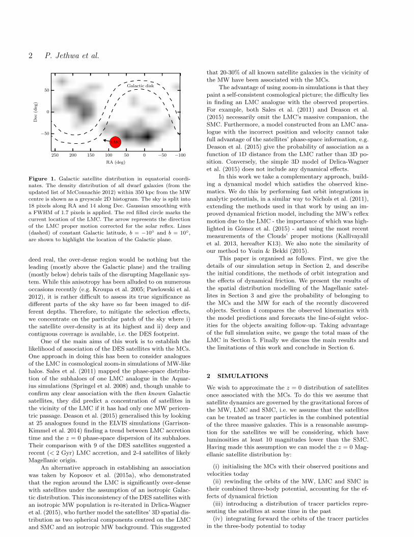
Table 3. Properties of satellites in the DES footprint. Values are

taken from (1) Koposov et al. (2015a) (2) Drlica-Wagner et al.

(2015) (3) Kim & Jerjen (2015).

Name l b D� MV Ref.

(deg) (deg) (kpc) (mag)

Columba 1 231.6 -28.9 182 -4.5 (2)

Grus 1 338.7 -58.2 120 -3.4 (1)Grus 2 351.1 -51.9 53 -3.9 (2)

Horologium 1 271.4 -54.7 79 -3.4 (1)

Horologium 2 262.5 -54.1 78 -2.6 (3)Indus 2 354.0 -37.4 214 -4.3 (1)

Phoenix 2 323.7 -59.7 83 -2.8 (1)

Pictoris 1 257.3 -40.6 115 -3.1 (1)Reticulum 2 266.3 -49.7 30 -2.7 (1)

Reticulum 3 273.9 -45.6 92 -3.3 (2)

Tucana 2 328.1 -52.3 58 -4.3 (1)Tucana 3 315.4 -56.2 25 -2.4 (2)

Tucana 4 313.3 -55.3 48 -3.5 (2)Tucana 5 316.3 -51.9 55 -1.6 (2)

their luminosity as function of distance, the right panel theiron-sky positions.

To compare our model with the observed satellites re-quires knowledge of the DES selection function. The esti-mated detection efficiencies of the satellites vary between1.0 and 0.2 (Drlica-Wagner et al. 2015) dependent on satel-lite distance, luminosity and size. Given the systematic un-certainties in determining these parameters (e.g. Koposovet al. (2015a) and Bechtol et al. (2015) give the luminosityof Reticulum 2 as MV = −2.7± 0.1 and −3.6± 0.1 respec-tively), there will be large uncertainties in reported detectionefficiencies. Guided by the sharp boundary between detec-tion and non-detection in efficiency maps calculated for theSloan Digital Sky Survey (SDSS) (Koposov et al. 2008), wecircumvent this uncertainty by assuming that detection is abinary decision. Furthermore, we assume that this decisionis determined entirely by distance and luminosity, omittingany dependence on size. In effect, this means that our re-sults will not account for any hypothetical population ofundetectably-low surface-brightness dwarfs. Our criteria fordetectability DES is thus

MV < MDESV,lim(D�)

= (1.45− log10(D�/kpc))/0.228. (17)

The slope of this relation is assumed equal to that calculatedfor SDSS (Koposov et al. 2009, i.e. Equation (18)) whilst theintersect is chosen such that all DES satellites lie above thisthreshold, as shown in the top left panel of Fig. 6.

In compiling Table 3, we have excluded all likely orknown globular clusters, along with the distant dwarf galaxycandidate Eridanus 2 which lies beyond the distance range ofour Magellanic satellite distributions (D� = 380 kpc). Wealso exclude the faintest dwarf candidate Cetus 2, at whoseluminosity (MV = 0 mag) our census of satellites is woefullyincomplete. The inclusion of Cetus 2 would therefore affectour results in a manner highly dependent on extrapolationsof the luminosity function well beyond current understand-ing.

3.2 Method

We now describe the steps we take to compare our simulatedMC satellites to the observed distribution.

3.2.1 MW Background

To allow for the possibility that some of the observed satel-lites do not have a Magellanic origin, we include an isotropicbackground component of MW satellites in our model. Theradial profile of this component is fixed to the ΛCDM pre-diction of the distribution of subhaloes, while we allow itsnormalisation to vary in a range informed by the number ofdwarfs observed in surveys prior to DES. Here we describethese choices.

The radial profile of our MW satellite background isgiven by the ΛCDM prediction of the number density of sub-haloes around MW-like host haloes (Springel et al. 2008),given by an Einasto parameters α = 0.68 and r−2 =0.81R200, where R200 is the virial radius of our MW model.We call this (un-normalised) profile νMW(r). In Section 6.1we will discuss the effect of loosening this assumption on theradial profile.

We parametrize the normalisation of the MW back-ground as a fraction of the value required to reproduce theobserved number of dwarfs discovered in SDSS Data Release5 (DR5, Adelman-McCarthy et al. 2008) with luminosities inthe range −7 < MV < −1. These are shown as black pointsin Fig. 6 (taken from McConnachie 2012). To determine therequired normalisation we must take into account the de-tectability threshold of DR5, which can be approximatedas a limiting luminosity as a function of distance (Koposovet al. 2009),

MDR5V,lim(D�) = (1.1− log10(D�/kpc))/0.228, (18)

shown as a black dashed line in the top left panel of Fig. 6.To determine what fraction of dwarfs are observable

subject to this criterion, we must assume a luminosity func-tion of dwarf galaxies L(MV ), i.e.

L(MV ) ∝ dn

dmsub

dmsub

dm∗

dm∗dL

dL

dMV. (19)

The first term of the right-hand side is given by the sub-halo mass function, N(M > msub) ∝ m−0.9

sub (e.g. Gao et al.2004; Springel et al. 2008). For the second term we assumem∗ ∝ mγ

sub, trying two values γ = 1.9 (Garrison-Kimmelet al. 2014, from abundance matching) and γ = 3 (Koposovet al. 2009, from fits to MW dwarfs). Inserting a constantstellar mass to light ratio and the standard definition of themagnitude scale into the third and fourth terms, and intro-ducing a normalising constant Kγ gives

L(MV ) = Kγ100.36MV /γ . (20)

where Kγ is chosen to ensure that L integrates to 1 in therange −7 < MV < −1. The median luminosities for ourtwo luminosity functions are MV = −2.9 for γ = 3 andMV = −2.4 for γ = 1.9, i.e. γ = 3 predicts more brightdwarfs.

The number of observable dwarfs within a distance D�is then given by the integral of the number density over theDR5 survey volume, V , within that distance, where we inte-grate the luminosity function down the faintest observable

c© 2015 RAS, MNRAS 000, 1–23

A Magellanic Origin of the DES Dwarfs 9

0 50 100 150 200 250 300 350

l (deg)

−50

0

50

b(d

eg)

LMC

SMC

−7

−6

−5

−4

−3

−2

−1

MV

DR5 limit

DES limit

DR5

DR10

PS3π

DES

101 102

D� (kpc)

100

101

102

N(<

r)

−100

DR5Nobs

Nexp

N4π

SDSS + PS3πNobs

Nexp

N4π

SDSS + PS3πNobs

Nexp

N4π

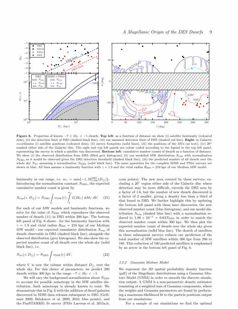
Figure 6. Properties of known −7 < MV < −1 dwarfs. Top left: as a function of distance we show (i) satellite luminosity (coloureddots), (ii) the detection limit of DR5 (dashed black line), (iii) our assumed detection limit of DES (dashed red line). Right: in Galactic

co-ordinates (i) satellite positions (coloured dots), (ii) survey footprints (solid lines), (iii) the positions of the MCs (as text), (iv) 20◦

masked either side of the Galactic disc. The right and top left panels are colour coded according to the legend in the top left panel,

representing the survey in which a satellite was discovered. Bottom left: cumulative number counts of dwarfs as a function of distance.

We show (i) the observed distribution from DR5 (filled grey histogram) (ii) our modelled MW distribution Nexp with normalisationNDR5 as it would be observed given the DR5 detection threshold (dashed black line), (iii) the predicted number of all dwarfs over the

whole sky N4π assuming a normalisation NDR5 (solid black line). The same quantities for the complete SDSS and PS3π surveys are

shown in blue. All lines assume a luminosity function with γ = 1.9 and the virial radius R200 = 210 kpc of our Medium MW model.

luminosity in our range, i.e. mv = min{−1,MDR5V,lim(D�)}.

Introducing the normalisation constant NDR5, the expectedcumulative number count is given by

Nexp(< D�) = NDR5

∫V

νMW(r)

mv∫−7

L(MV ) dMV dV. (21)

For each of our MW models and luminosity functions, wesolve for the value of NDR5 which reproduces the observednumber of dwarfs (11) in DR5 within 300 kpc. The bottomleft panel of Fig. 6 shows - for the luminosity function withγ = 1.9 and virial radius R200 = 210 kpc of our MediumMW model - our expected cumulative distribution Nexp ofdwarfs observable in DR5 (dashed black line), alongside theobserved distribution (grey histogram). We also show the ex-pected number count of all dwarfs over the whole sky (solidblack line), i.e.

N4π(< D�) = NDR5

∫V

νMW(r) dV, (22)

where V is now the volume within distance D� over thewhole sky. For this choice of parameters, we predict 280dwarfs within 300 kpc in the range −7 < MV < −1.

We will vary the background normalisation about NDR5

to account for possible anisotropy in the MW satellite dis-tribution. Such anisotropy is already known to exist. Wedemonstrate this in Fig. 6 with the addition of dwarf galaxiesdiscovered in SDSS data releases subsequent to DR5 (Grill-mair 2009; Belokurov et al. 2009, 2010, blue points), andthe PanSTARRS1 3π survey (PS3π Laevens et al. 2015a,b,

cyan points). The new area covered by these surveys, ex-cluding a 20◦ region either side of the Galactic disc wheredetection may be more difficult, exceeds the DR5 area bya factor of 1.6, but the number of new dwarfs discovered isa factor of 2 smaller, giving a density less than a third ofthat found in DR5. We further highlight this by updatingthe bottom left panel with these later discoveries: the newobserved number count (blue histogram), and our model dis-tribution Nexp (dashed blue line) with a normalisation re-duced to 1.98 × 10−3 = 0.63NDR5 in order to match theobserved number count within 300 kpc. We then plot theexpected number count of dwarfs over the whole sky giventhis normalisation (solid blue line). The dearth of satellitesin these subsequent surveys reduces our prediction of thetotal number of MW satellites within 300 kpc from 280 to180. This reduction of 100 predicted satellites is emphasisedby an arrow in the bottom left panel of Fig. 6.

3.2.2 Gaussian Mixture Model

We represent the 3D spatial probability density function(pdf) of the Magellanic distributions using a Gaussian Mix-ture Model (GMM) in order to smooth the discrete simula-tion output. A GMM is a non-parametric density estimatorconsisting of a weighted sum of Gaussian components, wherethe weights and Gaussian parameters are found by perform-ing a maximum-likelihood fit to the particle positions outputfrom our simulations.

For a sample of our simulations we find the optimal

c© 2015 RAS, MNRAS 000, 1–23

10 P. Jethwa et al.

number of GMM components, defined as the number whichminimises the Akaike information criterion. Each componentwas allowed an unconstrained covariance matrix This opti-mal number was found to be in the range 7-15, with theexact solution dependent on a variety of simulation parame-ters, e.g. LMC satellite distributions which have undergone1 MW crossing preferred fewer than 10 components, whilethose with multiple crossings preferred more than 10. Ratherthan performing the costly task of finding the optimal num-ber for each particular simulation, we chose to perform ouranalysis using 10 components for all of our simulated distri-butions.

For each combination of mass models we perform afull expectation-maximization fit for one simulation seededfrom a particular set of MC kinematics, then use the re-sulting GMM parameters to initialise fits for the remain-ing simulations which are completed using 30 expectation-maximization steps. A visual comparison of the samplesdrawn from the mixture models with the simulation out-put demonstrates that this fitting process is sufficient tocapture the differences in distributions as resolved by oursimulations.

3.2.3 Likelihood

We model the observed satellite distribution with three com-ponents: MW, LMC and SMC. The background MW modelhas a radial number density profile,

nMW(r) = fMWNDR5νMW(r), (23)

where r is Galactocentric distance and fMW is a normal-isation in units of the SDSS-DR5 satellite density. TheMCs have pdfs, fLMC(x,Θs) and fSMC(x,Θs), estimatedvia Gaussian Mixture Model, which are functions of Galac-tocentric Cartesian satellite position x and are dependenton simulation parameters Θs = (M,µ) where

M = (MMW,MLMC,MSMC), (24)

µ = (µLMCW , µLMC

N , µSMCW , µLMC

N ), (25)

i.e. the galaxy mass models and the MC proper motions,respectively. The pdfs further depend on whether the tracerparticles are initialised with either the cored or cusped dis-tribution. Introducing the parameters NLMC and NSMC,which we interpret as the total number of satellite galax-ies which have ever belonged to the LMC or SMC, oursatellite number density model, parametrized by Θ =(M,µ, fMW, NLMC, NSMC), is given by

F (x,Θ) = nMW(|x|)+NLMCfLMC(x,Θs)+NSMCfSMC(x,Θs).

(26)

Given a selection function S, a model f and data xi,the likelihood function L is generically given by (Richardsonet al. 2011)

logL = −∫S

f(x) dS +∑i

log f(xi), (27)

where the first term is a normalising integral and thesecond is a summation over data points. Our selectionfunction is the volume V of the DES footprint withinD� < 300 kpc where at each distance we consider only

pdf

1

10

100

NL

MC

+N

SM

C

Margenalised

Cored

Cusped

0.1 0.3 1

fMW

0.1

0.2

0.3

0.4

0.5

NSM

C/N

LM

C

1 10 100

NLMC +NSMC

0.1 0.2 0.3 0.4 0.5

NSMC/NLMC

Figure 7. Triangle plot showing marginalised 1D and 2D pos-

terior pdfs for the normalisation parameters of our model. Theparameters in columns, left to right, are the normalisation of the

MW background, the total number of Magellanic satellites, andthe fraction of SMC to LMC satellites. 1D posteriors show the

mean pdfs in black and the dependence on the results on the

initial density assumed for the satellite populations.

dwarfs brighter than the limiting observable luminositymv = min{−1,MDES

V,lim(D�)}, where MDESV,lim given by Equa-

tion (17), up to maximum luminosity MV = −7. To incor-porate this luminosity dependent selection function into ourmodel we must assume a luminosity function L(MV ), henceour full model is the product F (x,Θ)L(MV ). As in Sec-tion 3.2.1, we try two luminosity functions, given by Equa-tion (20) with indices γ = 1.9 or γ = 3, appending thisnuisance parameter to Θ. We assume that the shape of theMW and MC luminosity functions are the same. Our data,dDES = (x,MV ), consist of the Galactocentric Cartesian po-sitions and luminosities of the 14 satellites in Table 3. In-serting all of these terms into Equation (27), our likelihoodfunction is given by

logL(dDES|Θ) = −∫V

F (x,Θ)

∫ mv

−7

L(MV ) dMV dV

+

14∑i=1

log (F (xi,Θ)L(MV,i)) . (28)

3.2.4 Prior PDF

We now define the prior probability distribution on themodel parameters, P (Θ). We take a uniform prior over oursuite of simulations, in effect imposing a uniform prior overgalaxy mass models (see Table 1) and a Gaussian prior overproper motion measurements. Our prior on the normalisa-tion on the MW background fMW is uniform in log in therange [0.1, 3], where fMW = 1 gives a satellite density com-parable to that found in SDSS-DR5.

c© 2015 RAS, MNRAS 000, 1–23

A Magellanic Origin of the DES Dwarfs 11

The prior on the number of satellite galaxies of the LMCis given by

P (NLMC|MLMC) ∝

logNLMC if NLMC ≤ 10

(MLMC

1010M�

)0 otherwise

(29)

and likewise for the SMC. This prior is uniform in the logof number of satellite galaxies between zero and an upperlimit which is dependent on the galaxy mass, allowing ourlightest 2×1010M� LMC to have up to 20 satellites, whereasour most massive 3 × 1011M� LMC may have up to 300satellites. We justify this scaling of the feasible number ofsatellites with host mass since there is an approximatelylinear scaling between the number of subhaloes of a hosthalo and the mass of the host observed in ΛCDM simulations(e.g. Zentner et al. 2005).

As an order-of-magnitude justification of our upperlimit on satellite number, we consider the scaling betweenthe MW and our lightest LMC. Figure 6 shows that the ex-pected number of satellites within 300 kpc of the MW isaround 200 if we assume a density of satellite galaxies overthe entire sky similar to that found in the SDSS and PS3πsurveys. Our prior allows allow our lightest LMC to have asmany as 20 satellites: a factor of 10 fewer than estimatedfor the MW despite being a factor 50 less massive, which weconsider to be a reasonably broad prior given the uncertain-ties in populating subhaloes with satellite galaxies.

3.3 Results

We now examine the posterior probability distributions ofvarious parameters of interest. These are calculated by eval-uating the likelihood function on a grid, then using Bayes’theorem to calculate posterior probabilities,

P (Θ|dDES) =L(dDES|Θ)P (Θ)∫

ΘL(dDES|Θ)P (Θ) dΘ

, (30)

then marginalising as appropriate.Figure 7 shows the marginalised 1D and 2D posterior

pdfs for three of our model parameters: the normalisation ofthe MW component, the total number of Magellanic satel-lites, and the fraction of SMC to LMC satellites. In the 1Dposterior pdfs the black lines show the result marginalisedover two systematic uncertainties tested in our model, i.e.the initial density profile of MC satellites, and the luminosityfunction used.

We find that the results are insensitive to the choice ofluminosity function. We show the dependence of the resultson our choice of initial density profile using the colouredlines in Fig. 7. These show the marginalised posteriors whenwe use either the cusped (cyan) or cored (red) profiles. Wesee that the fully marginalised result more closely follow theresults derived from the cusped profile. This is because, with9 of our dozen satellites lying within 50 kpc of the LMC, ourfits generically prefer the more centrally concentrated initialdensity profile. Having only simulated two density slopeswe refrain from further discussion of the significance of thisresult. We discuss various other parameters, marginalisedover these systematic uncertainties, below.

0

1

PSM

C

Pictoris1

MW

Horologium1

MW

Horologium2

MW

0

1

PSM

C

Reticulum2

MW

Grus1

MW

Phoenix2

MW

0

1

PSM

C

Tucana2

MW

Reticulum3

MW

Tucana3

MW

0

1

PSM

C

Tucana4

MW

Tucana5

MW

Grus2

MW

0 1

PLMC

0

1

PSM

C

Columba1

MW

0 1

PLMC

Indus2

MW

0.001 0.01 0.1Probability

Figure 8. 2D satellite membership posterior pdfs, labelled per

panel. The bottom-left/bottom-right/top-left corner of each panelimply certain membership to the MW/LMC/SMC model compo-

nent respectively. Colours show the logarithmically scaled poste-rior pdf in the intervening space. Dotted lines demarcate regions

where a satellite is more likely a member of one component than

any other.

3.3.1 The Number of Magellanic Satellites

We constrain the total number of Magellanic satellites to be70+30−40, which are the mode and 68% confidence intervals of

the pdf shown in the central panel of Fig. 7. We stress thatthis is not an estimate of the number we predict to be stillbound to the MCs today, but refers to the total number ofsatellite galaxies which have evolved in the virial radii ofeither MC prior to their accretion onto the MW. Many ofthese predicted satellites will be in tails of tidally strippeddebris stretching far beyond the current extent of the matterbound to the MCs.

The bottom right panel of of Fig. 7 shows that weare unable to constrain the fraction of SMC to LMC satel-lites. This is in agreement with Drlica-Wagner et al. (2015)(henceforth DES15).

c© 2015 RAS, MNRAS 000, 1–23

12 P. Jethwa et al.

0.1

0.2

0.3

0.4

0.5

0.6

0.7

0.8

0.9

1.0

Pro

bab

ilit

y

Pic1

Hor1

Hor2

Ret2

Gru1

Pho2

Tuc2

Ret3

Tuc3

Tuc4

Tuc5

Gru2

Col1

Ind2

MW

LMC

SMC0 50 100 150 200

Distance from MW/LMC/SMC (kpc)

0.01

Figure 9. Probability of the observed satellites - as shown in the legend - belonging to the MW (black), LMC (red) or SMC (cyan)components of our model distribution, as a function of distance from the relevant host. While there are eight satellites more likely to

have originated in the LMC than the MW, there is only one satellite, Reticulum 3, with a modest probability of originating in the SMC.

3.3.2 The MW background

The left column panel of Fig. 7 shows a preference for a lowMW background. This suggests that most of the DES satel-lites are unlikely to be drawn from an isotropic MW pop-ulation. This conclusion was previously reached in DES15where a simple Kolmogorov-Smirnov test significantly re-jected this hypothesis. This can be seen by eye in the rightpanel of Fig. 6, where the on-sky positions of the DES satel-lites cluster around the MCs.

Quantitatively, our 68% (95%) confidence limits on theMW background are fMW < 0.40(0.87), in units of theaverage satellite density in SDSS-DR5 (discussed in Sec-tion 3.2.1). We convert this into a constraint on the numberof DES satellites belonging to the MW using the DES15 es-timate that roughly half of the DES detections would havebeen detected in SDSS. Accounting for this extra factor oftwo and the DES sky coverage in Equation (21), we arriveat a 68% (95%) confidence limit that fewer than 4 (8) of the14 DES satellites shown in Fig. 6 belong to an isotropic MWbackground.

Our constraint that fMW < 1 further implies that,once likely Magellanic satellites are excluded, the underlyingMW satellite population in DES is underdense compared toSDSS-DR5. The degree of anisotropy is weaker than thatinferred from comparison between SDSS-DR5 and DR10combined with PS3π (as discussed in Section 3.2.1) and,of course, presupposes that none of the SDSS-DR5 satellitesthemselves have a Magellanic origin.

3.3.3 Magellanic Probability of the DES satellites

We now calculate the probability of each observed satel-lite belonging to either the LMC or SMC component of ourmodel. For model parameters, Θ, the probability of a satel-lite at position x belonging to the LMC component is givenby

pL(x,Θ) =NLMCfLMC(x,Θs)

F (x,Θ), (31)

where the total model F (x,Θ) is defined in Equation (26).The SMC membership probability pS(x,Θ) is defined like-wise. From our simulations, we calculate the probabilityP (pL, pS |x,Θ) that a satellite at x has membership proba-bilites pL and pS for model parameters Θ. The 2D posteriorpdf for a satellite at x to have membership probabilities pLand pS , marginalised over Θ, is then given by

P (pL, pS |x,dDES) = (32)

1

(∗)

∫Θ

L(dDES|Θ)P (pL, pS |x,Θ)P (Θ) dΘ,

where (∗) is given by the denominator of Equation (30).Figure 8 shows the 2D membership probability pdfs cal-

culated at the position of all 14 DES satellites. Each panelrepresents the pdf for an individual satellite. We discussthree illustrative examples:

• Columba 1’s pdf peaks at PMW = 1 with a little prob-ability stretching towards LMC membership. Thus, we con-jecture that Columba 1 is likely a MW satellite.• Tucana 5’s pdf peaks at PLMC = 1, with a smaller peak

at PMW = 1, and some probability stretching away from thePMW = 0 axis. It is prudent to suppose that Tucana 5 couldwell be stripped from the LMC.• Reticulum 3’s looks similar to Tucana 5 but has a

prominent streak along PMW = 0, stretching well into thecorner of SMC membership. Therefore, there is some tanta-lizing evidence the Ret 3 could have been part of the SMC.

The information in Fig. 8 is summarised in Fig. 9 where,for each DES satellite, we sum the probability in the lociwhere it is more likely a member of the MW, LMC or SMCthan either other component (demarcated with dotted linesin Fig. 8) and plot this as a function of distance from therelevant host. Note a large number of satellites (likely of theLMC origin) for which the red filled symbol (the probabil-ity of belonging to the LMC) lies above the correspondingblack filled symbol (the MW membership). For such pairs,

c© 2015 RAS, MNRAS 000, 1–23

A Magellanic Origin of the DES Dwarfs 13

Table 4. DES satellites split by LMC membership probabilities.

LMC membership Satellites

pLMC > 0.7Ret2, Tuc2, Tuc4, Tuc5

Hor1, Hor2, Pho2

0.5 < pLMC < 0.7 Ret3, Tuc3, Gru1, Gru2, Pic1

pLMC < 0.2 Col1, Ind2

the distances from the LMC and the MW are sorted in anobvious manner: DLMC < DMW.

Table 4 summarises LMC membership probabilities forthe DES satellites, which we split into three bins comprising7 likely LMC members, 5 possible members and 2 unlikelymembers. Comparing with table 1 of Deason et al. (2015),we typically assign a slightly greater probability of LMCmembership (∆pLMC ∼ 0.2). We attribute this to the factthat the relative normalisation of the MW background is afree parameter in our model, whereas in Deason et al. (2015)it is fixed by their simulations.

3.3.4 Influence of the SMC?

Despite not being able to attribute an SMC origin to any ofthe DES satellites with a high probability, we can also askwhether its gravitational force has been influential for theorbital history of any of the DES satellites assuming theyhave an origin in the LMC satellite population. As a firstpass in answering this, we perform a further grid of simula-tions with no SMC, i.e. we simulate the LMC satellite pop-ulation in the potential of the MW and LMC only. Then,over the entire grid of simulations, we calculate the likeli-hood of the data, dDES, in the two component MW+LMCmodel, given by Equation (26) excluding the SMC compo-nent. Doing this, we discount the possibility that the SMChas its own satellites, but it still affects results through itsgravitational influence on LMC satellites.

Starting from a flat prior over the values the mass ra-tio MLMC/MSMC = (3, 5, 10,∞) (where ∞ means no SMC)gives a posterior pdf Pposterior = (0.29, 0.26, 0.25, 0.19). Theresult does not deviate greatly from the prior, however weslightly prefer every instance of the LMC populations whichhave experienced a massive SMC to those which have not.This very tentatively suggests that the SMC has had someinfluence over at least one of the DES satellites. We deferfurther investigation of this to later work.

3.3.5 Number of MW-LMC Pericenters

We can use the positions of the DES satellites to try to deter-mine the number of pericenters undergone between the MWand LMC in the last 11.5 Gyr. Our prior on this quantity,P (Nperi = n), comes from counting the fraction of MW-LMC orbits calculated, as described in Section 2.5, whichhave exactly n pericenters. Our posterior, given the observed

Table 5. Prior and posterior probability distributions on the

number of pericenters undergone between the MW and LMC in

the last 11.5 Gyr.

# MW-LMC pericenters Pprior Pposterior

1 0.64 0.90

2 0.29 0.10>2 0.07 < 10−3

positions of the DES satellites, is then

P (Nperi = n|dDES) = (33)

1

(∗)

∫Θ

L(dDES|Θ)P (Nperi = n|Θ)P (Θ) dΘ,

where the normalisation (∗) is given by the denominator ofEquation (30).

Table 5 shows the results. With the mass models wehave used for the MW and LMC, and the measurementsadopted for the LMC velocity, 64% of our orbit integrationsresult in a “first-passage” solution, where the LMC has onlyrecently (<0.1 Gyr ago) completed is first pericenter aboutthe MW. Updated with our knowledge of the positions ofthe DES satellites, the probability of a first-passage solutionincreases to 0.90. This is because at each pericenter the LMCundergoes an enhanced bout of tidal stripping, making it lesslikely to retain the localised concentration of satellites thathas been observed. This echoes the recent result of Deasonet al. (2015), that the DES satellites suggest a recent ac-cretion of the LMC onto the MW, as well as previous workswhich suggested that the LMC is on its first infall (e.g. Beslaet al. 2007).

Figure 4 shows that the number of MW-LMC peri-centers is primarily controlled by the mass of the MW.Our preference for “first-passage” solutions therefore con-verts into a preference for a low mass MW. For a flat priorover the three values, MMW

200 = (50, 100, 200)×1011M� givesPposterior = (0.65, 0.28, 0.07).

3.4 Maximum Likelihood 3D Model

Figure 10 shows the satellite distributions from our maxi-mum likelihood model. We show the on-sky distribution inMagellanic Stream (MS) co-ordinates (LMS, BMS) definedin Nidever et al. (2008), and in Galactocentric r againstLMS in two bins of BMS, for both the LMC and SMCcomponents. These have been generated from simulationsusing a cusped initial satellite distribution, galaxy masses(MMW,MLMC,MSMC) = (50, 12, 4) × 1010M�, and com-bining over all MC proper motions tried. The maximumlikelihood normalisations are fMW = 0.2, NLMC = 70 andNSMC = 1, for a luminosity function with γ = 1.9. We con-vert these figures into the expected number of observed satel-lites by integrating our satellite density models taking intoaccount the survey detection limit as given by Equation (17).Inside the entire DES volume, this results in expected num-bers of 10.8 observable LMC, 2.7 MW and fewer than 0.1SMC satellites.

Figure 11 shows the on-sky density of satellites for ourbackground MW model. The image in (LMS, BMS) shows the

c© 2015 RAS, MNRAS 000, 1–23

14 P. Jethwa et al.

−60

−40

−20

0

20

40

60

BM

S(d

eg)

b=

20

b=−

20 E(NSMC

obs ) < 0.1

b=

20

b=−

20 E(NLMC

obs ) = 10.8

20

40

60

80

100

120

r(k

pc)

5o < BMS < 25o

E(NSMCobs ) < 0.1

5o < BMS < 25o

E(NLMCobs ) = 5.0

−100−50050100

LMS (deg)

20

40

60

80

100

120

r(k

pc)

−30o < BMS < −10o

E(NSMCobs ) < 0.1

−100−50050100

LMS (deg)

−30o < BMS < −10o

E(NLMCobs ) = 1.2

0.01 0.01 0.03 0.06 0.12 0.23 0.46 0.92 1.8

SMC satellites

0.21 0.41 0.83 1.7 3.3 6.6 13 27 53

LMC satellites

Figure 10. Maximum likelihood model of the satellites of the SMC (left) and LMC (right). Top row: on-sky (LMS, BMS) projection

of (i) simulated satellite distribution (coloured contours), (ii) the LMC/SMC (large/small white circles), (iii) DES satellites (colouredsymbols defined in Fig. 9), (iv) DES footprint (solid line), (v) distribution of HI gas (faint contours), (vi) 20◦ either side of the Galactic

disk (dashed lines). Middle/bottom rows: distribution in LMS against Galactocentric r for bins 5◦ < BMS < 25◦ (middle) and

−30◦ < BMS < −10◦ (bottom). Contours step roughly in factors of 2 in projected density, with arbitrary units and colours comparableper column. For the maximum likelihood solution of ∼ 70 Magellanic satellites, the expected number of satellites observable by DES is

annotated in each panel.

quantity

f(LMS, BMS) =

300 kpc∫D�=0

nMW(r)D2� dD� (34)

where we have not included a cos(BMS) volume correctionfor clarity. Our MW component has a density gradient acrossthe DES footprint, being ∼ 20% greater in the south westcorner of the DES footprint (i.e. the bottom left corner ofthe plot) that the north east. This is due to the relativeproximity of the south west corner to the Galactic center. Aline of sight through this region therefore traverses more ofthe MW halo and has a greater probability of encounteringa MW satellite. Our model naturally accounts for this gra-dient, however we find it is not sufficient to account for theobserved distribution of the DES satellites and we require asignificant Magellanic contribution, as shown in Fig 9.

This maximum likelihood model assigns 12 of the DESsatellites a probability pL > 0.7 of belonging to the LMC,while the more distant Columba 1 and Indus 2 are most

likely to be MW satellites. The middle left panel of Fig. 10,we see that see that the distance of Reticulum 3 coincideswith the peak of the distribution of SMC satellites, makingit the only DES satellite with a non-negligible probabilityof belonging to the SMC. All other satellites are much morelikely to belong to the background MW population than tothe SMC.

Most of the remainder of the predicted LMC satellitesare located in a leading arm of debris stretching out behindthe Galactic disk. This is shown in equatorial co-ordinates inFig. 12, along with the footprints of SDSS, DES and ATLAS(Shanks et al. 2015) surveys. Much of the predicted lead-ing arm is currently lacking contiguous coverage, potentiallymaking the high Galactic latitude portion of the area shownin the figure a fruitful region for future satellite searches.Curiously, despite a rather patchy sky coverage, the Surveyof the Magellanic Stellar History (SMASH; PI D. Nidever)has already serendipitously unearthed the Hydra II dwarfgalaxy (Martin et al. 2015) at a position consistent with theLMC leading tail. The Galactocentric distances of our sim-

c© 2015 RAS, MNRAS 000, 1–23

A Magellanic Origin of the DES Dwarfs 15

−120−100−80−60−40−20020

LMS (deg)

−60

−40

−20

0

20

40

60

BM

S(d

eg)

E(NMWobs ) = 2.7

0.64 0.68 0.72 0.76 0.80

MW satellites

Figure 11. On-sky density model of MW dwarfs. Symbols show

DES satellites, defined in Fig. 9. We also show the DES footprint,

and label the expected number of MW satellites observable inDES.

−70.0◦

−50.0◦

−30.0◦

−10.0◦

80◦

100◦120◦140◦

160◦

180◦

LMC

Hydra 2

SDSS

VST−ATLAS

DES

Galac

ticDisk

RA

:Dec.

Figure 12. Leading arm of Magellanic satellites shown in

equatorial coordinates in a gnomic projection centred on (RA,

Dec.)=(130◦,−50◦). Filled coloured contours represent the dis-tribution of satellites from our maximum likelihood model inte-

grated along the line of sight. Footprints of the SDSS, DES, and

ATLAS surveys are shown alongside lines of constant Galacticlatitude at b = −10◦ and b = 10◦. The solid black line tracing

the centre of the distribution is a segment of the great circle withpole (RA, Dec.)=(275◦,−41◦). Black dots show the positions of

known satellites, with the LMC and Hydra 2 labelled.

ulated leading arm of satellites peak in the range 40-80 kpc,albeit extending as far as 300 kpc.

While our model can reproduce the number of satel-lites discovered, there is tension regarding their distributionwithin the DES footprint. The top right panel of Fig. 10shows that our model predicts a concentration of satelliteswithin 10 kpc of the LMC, which is not present in the data.This might be a result of our over-simplistic treatment of thetidal disruption of satellites. The stellar disk of the LMC ex-tends beyond 10 kpc from its centre (e.g. van der Marel &

−100

−60

−20

20

Y(k

pc)

LMCSMC

XY

−60 −20 20 60

X (kpc)

−140

−100

−60

−20

Z(k

pc)

Edge On

−100 −60 −20 20

Y (kpc)

Face On

0 2 4 6 8 10 12

rrms (kpc)

Figure 13. Distribution of BMS > 0◦ satellites (red) and BMS <

0◦ (cyan) in rotated Galactocentric Cartesian co-ordinates. The

LMC/SMC are shown by the large/small white circles, the pro-jection of the volume limited by the DES footprint is shown in

grey-scale. The top right panel shows the distribution of root-

mean-squared distances of groups of 7 low BMS satellite analoguesfrom our simulations, with the observed value in red. We conclude

that the observed plane has a significance of 95%

Kallivayalil 2014), hence satellite destruction is likely to oc-cur at distances greater than the 5 kpc zone-of-avoidancewe have naively imposed in our model. For our maximumlikelihood model, the fraction of particles today within 10,15 and 20 kpc of the LMC is 3, 8 and 14 % respectively; ac-counting for destruction of satellite which have, at any time,entered within these distances would reduce our predictionof the total number of Magellanic satellites by at least theseproportions.

A further failure of our model is the under-predictionof satellites in the range −30◦ < BMS < −10◦. Our maxi-mum likelihood model predicts 1.2 satellites in this range,whereas 7 are observed. Even allowing for the possibilitythat some of these belong to a background MW population,this suggests an over-density of satellites in a small spa-tial region compared to expectations from the disruption ofan isotropic LMC satellite population. Furthermore, despitetheir on-sky proximity to the SMC, Fig. 9 shows that 5 ofthese 7 low BMS satellites (Tucana 2-5 and Grus 2) are infact the least likely candidates to have belonged to the SMC.This is due to their distances (r < 60 kpc) being incompat-ible with satellites stripped from the SMC halo, as seen inthe bottom left panel of Fig. 10.

3.5 A Plane of LMC Satellites?

We now investigate this hint of an anisotropy in the LMCsatellite population. We investigate whether the seven DESsatellites observed at BMS < 0◦ reside in a coherent struc-ture, namely a thin plane as has been observed amongst the

c© 2015 RAS, MNRAS 000, 1–23

16 P. Jethwa et al.

satellites of both the MW (e.g. Kroupa et al. 2005) and M31(Ibata et al. 2013). We test 104 normal vectors spaced uni-formly around the unit sphere to find the plane containingthe LMC which minimises the root-mean-squared (rms) dis-tance of the seven BMS < 0◦ DES satellites. The resultingplane has an rms thickness of 2.7 kpc, with a radial extentof 90 kpc to the most distant satellite, Grus 1. The SMC hasa minimum distance of 2.0 kpc from the plane.

Figure 13 shows the satellite distribution in Galacto-centric Cartesian co-ordinates (X, Y , Z), which have beenrotated by 20.94◦ about the Z-axis such that the best-fitplane is edge-on in the (X, Z) projection. We also show theprojection of the volume limited by the DES footprint, whichappears to coincide with the plane in the (X, Z) projection.This is a mere coincidence, since the low BMS satellites donot lie near the footprint edges, as can be seen in Fig. 10.

We test the significance of this observed satellite planeby comparing to our simulations. We take our maximumlikelihood model and consider all the particles representingLMC satellites in the box −50◦ < LMS < −25◦, −30◦ <BMS < −10◦, which number around 104. We then consider104 random samples of 7 of these particles, insisting that theparticle furthest from the LMC has a distance within 90-100 kpc, similar to Grus 1 at 93 kpc. We perform the sameplane fitting procedure on the random samples as with theobserved satellites. The top right panel of Fig. 13 shows thedistribution of the resulting rms distances. Finding a planeat least as thin as the one observed occurs 5% of the timewhen sampling from our simulations, i.e. the plane has asignificance of 95%.

This calculation does not take into the account the factthat some of the low BMS satellites may not be genuineLMC satellites. Figure 9 shows that three of these (Tucana3, Grus 1 and Grus 2) have MW membership probabilities> 0.5. None are likely SMC candidates. Accounting for theiruncertain origin, then, would increase the significance (andcoincidental nature!) of the observed LMC satellite plane,since the distance distribution of MW satellites is broaderthan that of LMC satellites.

The observation of this plane is thus quite surprising.Given a population of satellites which is initially distributedisotropically about the LMC, then evolved in the combinedpotentials of the MW, LMC and SMC, it is a rare occu-rance to find 7 satellites - selected on similar criteria to theobserved ones - exhibiting the observed degree of planarity.

4 MODEL FOR THE VELOCITYDISTRIBUTION

We now consider the velocity information contained in ourmodel. To recap, the velocities of our simulated satellite arecomposed of the orbital velocity of the LMC or SMC aboutthe MW (or indeed the SMC about the LMC), a dispersioninherent in our simulated MC haloes, and a component in-duced by the potential of the MW for any satellite whichhas been, or is in the process of being, tidally stripped fromits host. In addition to their configuration-space positions,satellite velocity information can act as a discriminant ofmembership to the MCs, and trace the gravitational poten-tial of their host at distances unprobed by other luminoustracers.

−400

−300

−200

−100

0

100

200

300

400

vG

SR

(km

s−1)

SMC satellites

−100−50050100

LMS (deg)

−400

−300

−200

−100

0

100

200

300

400

vG

SR

(km

s−1)

LMC satellites

Figure 14. Distributions in GSR line-of-sight velocity against

LMS. Filled contours represent the simulated satellites for our

maximum likelihood model of SMC (top) and LMC (bottom),coloured symbols show the positions of four DES satellites (given

in the legend of Fig. 9), large/small white circles show the position

of the LMC/SMC, black contours show the distribution of HI gasfrom Nidever et al. (2008).

In this section we will look at the phase-space dis-tribution of our maximum likelihood model, then derivemarginalised velocity predictions for the DES satellites as-suming their membership to the MCs.

4.1 Maximum Likelihood Model for Kinematics

Figure 14 shows a projection of the phase-space distributionof the LMC and SMC satellite populations of our maximumlikelihood model defined in Section 3.4. We show the dis-tribution in LMS against vGSR, the line-of-sight velocity inthe Galactic standard of rest (GSR). We also show the posi-tions of the MCs and the positions of the four DES satelliteswith measured line-of-sight velocities which are given in therightmost column of Table 6.

Viewed in this projection, all four DES satellites withmeasured velocities appear consistent with the simulatedLMC satellite distribution. Furthermore, Tucana 2 and Grus1 (at LMS ≈ −40◦) have more negative velocities thanHorologium 1 and Reticulum 2 (at LMS ≈ −20◦). This isconsistent with the velocity trend seen in the simulated trail-ing arm of LMC satellites, bolstering the case for their mem-bership to this population.

4.2 Comparison to HI gas

Figure 14 also shows is the distribution of HI gas taken fromNidever et al. (2008) overplotted as black contours. Contourlevels step logarithmically, with line thickness representingdensity projected in the (LMS, vGSR) plane. This distributioncomprises gas within the LMC and SMC, a bridge of gas

c© 2015 RAS, MNRAS 000, 1–23

A Magellanic Origin of the DES Dwarfs 17

connecting the two, the trailing Magellanic Stream (MS) atlongitudes LMS < 0◦, and a few complexes comprising theLeading Arm (LA) at longitudes LMS > 0◦.

We see that the MS gas (at LMS < 0◦) is systematicallyoffset from the observed LMC satellite velocites by some 100-150 km s−1. Assuming a scenario where the LMC originallyplayed host to some or all of the MS gas (as proposed inNidever et al. 2008), and the satellites (as proposed here),this offset may be the result of ram-pressure stripping ofthe MS gas by the hot MW halo gas, an effect to which thesatellite orbits remain impervious.

Alternatively, this offset may be the result of the MSoriginating in the SMC rather than the LMC. Indeed, themodels of both Besla et al. (2012) and Diaz & Bekki (2012)show that tidal stripping of gas from the SMC is able to re-produce morphological and kinematic properties of the MS.Though these models tidally strip gas from a rotating SMCdisc, whereas we strip satellites from an isotropic sphericaldistribution, the fact that the MS and our simulated SMCsatellite kinematics are broadly comparable, as shown in thetop panel of Fig. 14, is reassuring.

We also mention the recent MS production model ofHammer et al. (2015), which invokes a collision between theMCs and ram-pressure stripping to successfully reproducemany morphological and kinematic properties of the MS.Given the inability of ram-pressure to pull gas in front ofthe MC orbits, they propose that the Leading Arm (LA)may be the result of “successive passages of leading, smalldwarfs that have lost their gas from ram pressure”. Fig. 10shows that the on-sky positions of the gas complexes com-prising the LA are comfortably within the scope of our sim-ulated LMC satellite distribution, hence we believe that theLA production scenario described in Hammer et al. (2015)is well accommodated in the picture of Magellanic group in-fall. Hammer et al. (2015) presuppose that the inferred timegap between the arrival to the MW of the dwarfs and theMCs precludes their belonging to group, however this failsto consider the possibility of very massive (M200 > 1011M�)and extended LMC dark halo.

4.3 Velocity predictions

We now predict the velocities of the DES satellites underthe assumption that they were members of one of the MCs,marginalised over our entire grid of models. For each of oursimulations, Θ, we approximate the local velocity distribu-tion at position x assuming membership to the LMC popu-lation - which we call P (v|x,Θ,LMC) - as a normal distribu-tion with mean and standard deviation given by the veloci-ties of the ten LMC satellite tracers nearest to x, excludingany three-sigma velocity outliers. We then marginalise overmodel parameters to give velocity pdfs for a satellite at x,assuming it belongs to the LMC,

P (v|x, dDES,LMC) = (35)

1

(∗)

∫Θ

L(dDES|Θ)P (v|x,Θ,LMC)P (Θ) dΘ,

where (∗) is the denominator of Equation (30), and we havealso incorporated the information provided by the positionaldata dDES. We derive velocity prediction assuming SMCmembership similarly.

pdf Reticulum2

pdf Tucana2

pdf Grus1

pdf Horologium1

−400 −300 −200 −100 0 100 200 300 400

vGSR (km s−1)

pdf Reticulum3 LMC

SMC

Figure 15. Predictions for the GSR line-of-sight velocity for five

of the DES satellites as labelled in each panel. The y-axis ranges

from 0 to 0.007 in each panel. The red/cyan distributions arepredictions assuming membership to the LMC/SMC populations.

The black vertical lines show measured values.

Table 6 shows our resulting predictions the for line-of-sight velocity and two components of proper motions in thesolar rest-frame. We report the maximum likelihood valuesalong with the 68% and 95% confidence intervals. The right-most column shows measured values where available. Fig 15shows the predictions assuming LMC membership, trans-formed into GSR, for the four satellites with measured line-of-sight velocities. The breadth of these distributions is dueto the combination of the inherent velocity dispersion in ourMC haloes and the spread in possible MC orbital histories.We see that all four measured velocities are consistent withbeing drawn from the LMC population at the 2σ level. Inparticular, Horologium 1 lies at the peak of its LMC satellitevelocity prediction, taking its probability of LMC member-ship beyond reasonable doubt.

The bottom panel of Fig. 15 shows the predictions forReticulum 3, the one satellite with a reasonable chance ofbelonging to the SMC population based on its position, ac-cording to Fig. 9. Though the velocity distributions assum-ing LMC and SMC membership are somewhat coincident, ameasurement of vGSR > 100 km s−1 (i.e. vhel > 270 km s−1)for Reticulum 3 would increase the likelihood of its belong-ing to the SMC. As will discuss in Section 6, proper motionswould also help us understand their origin.

5 THE MASS OF THE LMC

While the enclosed mass of the LMC is well constrained atM(< 8.7 kpc) = (1.7 ± 0.7) × 1010M� (van der Marel &Kallivayalil 2014), its total mass remains largely unknown.Abundance-matching would suggest that a galaxy with thestellar mass of ∼ 2.9× 109M�, equal to that of the LMC’s(van der Marel et al. 2002), are likely to reside in haloeswith a virial mass of 2× 1011M� (Moster et al. 2013). Ev-idence for such a mass, however, is scarce. Circumstantial

c© 2015 RAS, MNRAS 000, 1–23

18 P. Jethwa et al.

Table 6. Satellite velocity predictions and measurements. Predictions are given for line-of-sight velocity vhel and proper motions (µW , µN )

in the solar rest-frame, assuming membership to the LMC (columns 2-4) and SMC (columns 5-7). We highlight the SMC prediction forthe most likely candidate, Reticulum 3. Predictions are given as a maximum likelihood value with asymmetric errors indicating the 68%

(95%) confidence intervals. Column 8 shows measured line-of-sight velocities from (1) Koposov et al. (2015b) (2) Walker et al. (2015).

LMC Predictions SMC Predictions Observed

Name vhel µW µN vhel µW µN vhel

(km s−1) (mas yr−1) (mas yr−1) (km s−1) (mas yr−1) (mas yr−1) (km s−1)

Pic1 245+87(180)−66(148)

−0.22+0.17(0.38)−0.19(0.41)

−0.87+0.16(0.39)−0.15(0.33)

344+70(151)−84(596)

−0.50+0.36(0.64)−0.17(0.62)

−0.71+0.17(0.72)−0.16(0.41)

-

Hor1 124+88(204)−70(157)

−0.75+0.25(0.57)−0.27(0.59)

−1.28+0.20(0.45)−0.24(0.51)

270+87(188)−76(526)

−1.08+0.40(1.08)−0.22(0.59)

−0.97+0.22(0.98)−0.20(0.46)

112.8(1)

Hor2 133+89(202)−71(158)

−0.71+0.26(0.58)−0.27(0.60)

−1.32+0.20(0.45)−0.24(0.51)

271+87(190)−75(528)

−1.09+0.37(1.09)−0.23(0.64)

−0.99+0.22(1.00)−0.20(0.48)

-

Ret2 186+125(288)−107(237)

−1.37+1.46(2.98)−1.20(2.77)

−3.34+1.02(2.10)−0.74(1.71)

362+147(329)−194(660)

−0.00+−0.32(1.48)−3.63(5.54)

0.02+−1.01(0.13)−3.22(4.49)

64.7(1)

Gru1 −61+84(187)−65(139)

−0.93+0.12(0.29)−0.17(0.35)

−0.27+0.15(0.32)−0.16(0.33)

42+101(297)−95(332)

−0.87+0.12(0.86)−0.22(0.58)

−0.23+0.14(0.31)−0.20(0.64)

-140.5(2)

Pho2 −30+82(193)−71(157)

−1.33+0.19(0.43)−0.26(0.54)

−0.61+0.25(0.55)−0.27(0.58)

133+105(244)−114(418)

−1.31+0.27(1.31)−0.34(0.71)

−0.55+0.23(0.58)−0.27(0.63)

-

Tuc2 −34+110(256)−80(181)

−2.09+0.31(0.76)−0.41(0.89)

−0.58+0.47(1.09)−0.52(1.18)

169+126(272)−153(486)

−0.00+−1.26(0.00)−2.50(3.15)

0.02+−0.25(0.27)−1.23(1.84)

-129.1(2)

Ret3 205+88(196)−66(148)

−0.37+0.22(0.49)−0.24(0.52)

−1.11+0.16(0.39)−0.20(0.41)

330+68(155)−68(584)

−0.56+0.26(0.59)−0.27(0.67)

−0.86+0.15(0.87)−0.18(0.40)

-

Tuc3 47+188(396)−148(332)

−3.77+2.72(5.67)−1.54(3.71)

−2.20+2.11(4.89)−1.78(4.14)

277+186(435)−289(681)

−0.00+−0.46(1.99)−5.45(8.03)

0.02+0.03(2.90)−3.35(5.69)

-

Tuc4 14+125(278)−86(196)

−2.28+0.53(1.34)−0.52(1.17)

−1.34+0.61(1.41)−0.63(1.39)

250+116(269)−182(559)

−0.00+−1.20(0.01)−2.80(3.62)

0.02+−0.60(0.07)−1.79(2.57)

-

Tuc5 17+112(257)−82(183)

−2.05+0.38(0.94)−0.44(0.96)

−0.96+0.51(1.20)−0.57(1.25)

227+116(256)−156(520)

−0.00+−1.14(0.00)−2.40(3.06)

0.02+−0.43(0.11)−1.44(2.05)

-

Gru2 −143+130(308)−86(196)

−2.30+0.41(0.94)−0.51(1.11)

−0.27+0.52(1.16)−0.54(1.27)

38+182(377)−172(458)

−0.00+−1.47(0.00)−3.08(4.00)

0.02+−0.05(0.68)−1.22(2.05)

-

Cet2 −171+206(451)−154(333)

−2.82+1.04(2.52)−1.26(2.85)

−2.38+1.01(2.26)−1.18(2.57)

−53+239(516)−201(473)

−0.00+−1.75(0.02)−4.76(6.60)

0.02+−0.99(0.02)−2.94(4.38)

-

Col1 265+91(186)−88(203)

−0.21+0.17(0.35)−0.12(0.27)

−0.50+0.25(0.47)−0.11(0.29)

339+91(186)−137(590)

−0.00+0.01(0.27)−0.63(1.23)

−0.46+0.25(0.48)−0.23(0.59)

-

Ind2 −79+95(208)−63(139)

−0.53+0.09(0.27)−0.11(0.26)

0.08+0.09(0.18)−0.12(0.25)

−32+144(373)−94(289)

−0.53+0.08(0.53)−0.21(0.65)

0.02+0.16(0.29)−0.15(0.80)

-

evidence comes from models of the Magellanic Stream for-mation which require the LMC and SMC to form a long-livedbinary pair (Besla et al. 2012), which is the favoured sce-nario for > 1011M� LMCs (K13). Penarrubia et al. (2016)attempted a direct measurement by modelling the LMC’sdynamical effect on galaxies in the Local Volume. They in-ferred a mass 2.5 ± 0.9 × 1011M�, but stressed this resultmust be treated with caution due to the simplifying assump-tions necessary in their analysis.

The LMC’s satellite galaxies, acting as tracers of itsgravitational potential at large distances, offer a new line ofinquiry. Having demonstrated, in Section 3, that many ofthe DES satellites have a high probability of belonging tosuch a population of LMC satellites, we will now try to usethem to infer the LMC mass.

5.1 MLMC estimate based on positions only

We first ask what constraints we can put on the LMC massbefore assuming membership or otherwise of any satelliteto the LMC population. We calculate the posterior pdf ofMLMC from our three component (MW+LMC+SMC) 3D

spatial distribution model

, P (MLMC|dDES) =1

(∗)

∫Θ

L(dDES|Θ)P (MLMC|Θ)P (Θ)dΘ,

(36)

where (∗) is the denominator of Equation (30).The top panel of Fig. 16 shows the result. The poste-

rior is broadly flat, which may be expected when attempt-ing to constrain a galaxy’s mass without the use of veloc-ity information. There is, however, a small peak between4 ≤MLMC/1010M� ≤ 6 whose origin we briefly discuss.

The constraining power at the low mass end is the com-bined result of two effects. Firstly, our lowest mass LMCmodel is likely to play host to the fewest number of satel-lites, which we impose via the prior shown in Equation (29).Secondly, the same LMC is also the most likely to undergomultiple pericentric passages with the MW, seen in Fig. 4, asa result of the mass dependence of dynamical friction. Thelikely fate for the relatively few satellites of a 2 × 1010M�LMC, then, is to be tidally stripped from their host during aprevious close approach with the MW, in slight tension withthe observed concentration of satellites around the LMC.

The constraining power at the high mass end comesfrom the extent of the observed satellite distribution. Ascan be seen in Fig. 9, 12 out of 14 DES satellites are within

c© 2015 RAS, MNRAS 000, 1–23

A Magellanic Origin of the DES Dwarfs 19

10−3

10−2

10−1

pdf

Positions

10−3

10−2

10−1

pdf

Positions + 3 Velocities

(No Gru1)

2 4 6 8 10 12 14 16 18 20 22 24 26 28 30

MLMC (1010M�)

10−3

10−2

10−1

pdf

Positions + 4 Velocities

Figure 16. Posterior pdfs on the virial mass of the LMC halo.

The top row uses just the positions of the DES satellites, the mid-

dle/bottom rows include velocity information from 3/4 satellites.Dashed/dotted black lines show the results using cored/cuspy ini-

tial conditions, solid lines show the marginalised result, red line

shows the flat prior. The shaded region in the bottom panel showsthe 68% confidence interval about the most likely value.

100 kpc of the LMC, while 9 are within 50 kpc. Given thatour simulated satellite distributions extend out to the virialradius of their host, we slightly disfavour very massive LMCswhich have virial radii extending far beyond the observedsatellite distribution.

5.2 MLMC estimate using velocity information

We now make the assumption that some of the DES satellitesare indeed satellites of the LMC, and use their measured ve-locities to constrain its mass. Section 3.3.3 shows that basedon their 3D positions alone, of the four satellites with mea-sured velocities, three are likely members of the LMC whileone, Grus 1, is a possible member. We therefore performthis analysis both with and without Grus 1. It is importantto note that our assumption here is that the satellites haveexisted in the LMC halo at some point, not the strongerstatement that they are still bound to the LMC today. Oursimulations explicitly include satellites which have been, orare currently being, tidally stripped from the LMC by theMW.

To incorporate the velocity information we define a newlikelihood function. Of the 14 satellites whose positions inSection 3, we have now assumed that N of these, which havemeasured velocities, are LMC satellites. Our new, combineddata set thus comprises

(i) dL = {xL,MV,L, vL}: the positions, luminosities andvelocities of N satellites assumed to belong to the LMC

(ii) d = {x,MV }: the positions and luminosities of theremaining DES satellites

The new likelihood function is given by

logL(d, dL|Θ) = Equation (28) summed over d + (37)

N∑i=1

logFL(xiL) +

N∑i=1

logP (viL|xiL,Θ,LMC),

where Equation (28) refers to the original likelihood us-ing just positional data, FL(x) is LMC component of oursatellite distribution model given by Equation (26), andP (v|x,Θ,LMC) are the the local velocity distributions ap-proximated from the simulations as described in Section 4.We calculate posteriors on MLMC using this new likelihood.

The bottom two rows of Fig. 16 show the result when weinclude velocity information. In each panel the dashed anddotted lines show the results when we use the cored or cuspysatellite populations respectively, while the solid line showsthe marginalised result. As in Fig. 7, the mean posteriorclosely follows the results using the cusped profile since thesetypically provide better fits to the data. Despite the variationbetween results dependent on our choice of initial satellitedensity profile, and a level of noise seeded from noise in oursimulations, we find that some trend persists.

The addition of the 3 velocities of likely LMC satellitesleads us to slightly favour masses MLMC < 14 × 1010M�.This weak upper bound is mainly driven by Horologium1 which, as discussed in Koposov et al. (2015b), has aline-of-sight velocity just 15 km s−1 discrepant from thevalue expected at its position if it were stationary withrespect to the LMC. Such a low relative velocity is morelikely to occur in lighter LMCs, which have smaller halovelocity dispersions. The addition of Grus 1 to our veloc-ity sample creates a peak in the posteriors in the range10 ≤ MLMC/1010M� ≤ 12, and leads us to strongly dis-favour the lightest LMC,MLMC = 2×1010M�, which we dis-cuss below. Assuming all four satellites do indeed belong tothe LMC, the most likely value and 68% confidence intervalfor the LMC halo mass is given by MLMC = 12+8

−7×1010M�.

5.3 Grus 1

Figure 17 demonstrates how the inclusion of Grus 1 imposesa lower bound on the LMC mass. We take simulations of alight and heavy LMC, with masses of 2 and 12 ×1010M�respectively, with all other model parameters kept fixed. Forparticles inside the DES footprint, we plot the phase spacedistributions in Galactocentric r against vGSR, and over-plot the phase space positions of the DES satellites withmeasured velocities. At the distance of Grus 1, the satellitedistribution for the light LMC does not extend to sufficientlynegative velocities to accommodate Grus 1, yet it is wellwithin the scope of the heavy LMC’s distribution.

There are two reasons for this. Firstly, the satellites ofthe heavy LMC comprise a hotter population than those ofthe light LMC, filling a larger volume of the available phasespace. The second reason is due to the mass dependence ofthe LMC’s orbital history, demonstrated in the right panelof Fig. 17 where we compare the past orbits of the light LMC(dashed line) with that of the heavy LMC (solid line). Bothare calculated in the potential of our Light MW model forz = 0 velocities given by the central values in Table 2. Inte-grating backwards from this fixed velocity, dynamical fric-tion accelerates the LMC along its orbit. The heavy LMC,

c© 2015 RAS, MNRAS 000, 1–23

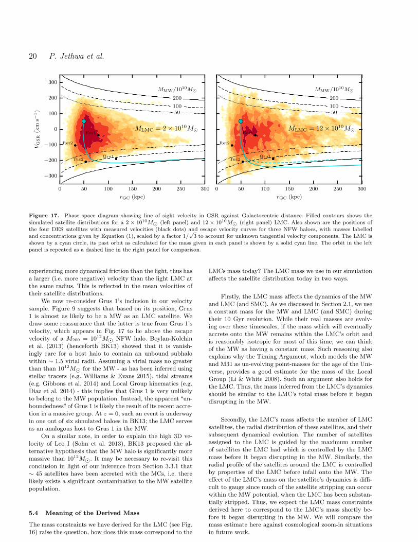
20 P. Jethwa et al.

0 50 100 150 200 250 300

rGC (kpc)

−300

−200

−100

0

100

200

300

VG

SR

(km

s−1) 50

100

200

MMW/1010M�

Hor1

Ret2

Gru1Tuc2

MLMC = 2× 1010M�

0 50 100 150 200 250 300

rGC (kpc)

50100

200

MMW/1010M�

Hor1

Ret2

Gru1Tuc2

MLMC = 12× 1010M�

Figure 17. Phase space diagram showing line of sight velocity in GSR against Galactocentric distance. Filled contours shows the

simulated satellite distributions for a 2 × 1010M� (left panel) and 12 × 1010M� (right panel) LMC. Also shown are the positions ofthe four DES satellites with measured velocities (black dots) and escape velocity curves for three NFW haloes, with masses labelled

and concentrations given by Equation (1), scaled by a factor 1/√

3 to account for unknown tangential velocity components. The LMC isshown by a cyan circle, its past orbit as calculated for the mass given in each panel is shown by a solid cyan line. The orbit in the left

panel is repeated as a dashed line in the right panel for comparison.

experiencing more dynamical friction than the light, thus hasa larger (i.e. more negative) velocity than the light LMC atthe same radius. This is reflected in the mean velocities oftheir satellite distributions.

We now re-consider Grus 1’s inclusion in our velocitysample. Figure 9 suggests that based on its position, Grus1 is almost as likely to be a MW as an LMC satellite. Wedraw some reassurance that the latter is true from Grus 1’svelocity, which appears in Fig. 17 to lie above the escapevelocity of a M200 = 1012M� NFW halo. Boylan-Kolchinet al. (2013) (henceforth BK13) showed that it is vanish-ingly rare for a host halo to contain an unbound subhalowithin ∼ 1.5 virial radii. Assuming a virial mass no greaterthan than 1012M� for the MW - as has been inferred usingstellar tracers (e.g. Williams & Evans 2015), tidal streams(e.g. Gibbons et al. 2014) and Local Group kinematics (e.g.Diaz et al. 2014) - this implies that Grus 1 is very unlikelyto belong to the MW population. Instead, the apparent “un-boundedness”of Grus 1 is likely the result of its recent accre-tion in a massive group. At z = 0, such an event is underwayin one out of six simulated haloes in BK13; the LMC servesas an analogous host to Grus 1 in the MW.

On a similar note, in order to explain the high 3D ve-locity of Leo I (Sohn et al. 2013), BK13 proposed the al-ternative hypothesis that the MW halo is significantly moremassive than 1012M�. It may be necessary to re-visit thisconclusion in light of our inference from Section 3.3.1 that∼ 45 satellites have been accreted with the MCs, i.e. therelikely exists a significant contamination to the MW satellitepopulation.

5.4 Meaning of the Derived Mass

The mass constraints we have derived for the LMC (see Fig.16) raise the question, how does this mass correspond to the

LMCs mass today? The LMC mass we use in our simulationaffects the satellite distribution today in two ways.

Firstly, the LMC mass affects the dynamics of the MWand LMC (and SMC). As we discussed in Section 2.1, we usea constant mass for the MW and LMC (and SMC) duringtheir 10 Gyr evolution. While their real masses are evolv-ing over these timescales, if the mass which will eventuallyaccrete onto the MW remains within the LMC’s orbit andis reasonably isotropic for most of this time, we can thinkof the MW as having a constant mass. Such reasoning alsoexplains why the Timing Argument, which models the MWand M31 as un-evolving point-masses for the age of the Uni-verse, provides a good estimate for the mass of the LocalGroup (Li & White 2008). Such an argument also holds forthe LMC. Thus, the mass inferred from the LMC’s dynamicsshould be similar to the LMC’s total mass before it begandisrupting in the MW.

Secondly, the LMC’s mass affects the number of LMCsatellites, the radial distribution of these satellites, and theirsubsequent dynamical evolution. The number of satellitesassigned to the LMC is guided by the maximum numberof satellites the LMC had which is controlled by the LMCmass before it began disrupting in the MW. Similarly, theradial profile of the satellites around the LMC is controlledby properties of the LMC before infall onto the MW. Theeffect of the LMC’s mass on the satellite’s dynamics is diffi-cult to gauge since much of the satellite stripping can occurwithin the MW potential, when the LMC has been substan-tially stripped. Thus, we expect the LMC mass constraintsderived here to correspond to the LMC’s mass shortly be-fore it began disrupting in the MW. We will compare themass estimate here against cosmological zoom-in situationsin future work.

c© 2015 RAS, MNRAS 000, 1–23

A Magellanic Origin of the DES Dwarfs 21

6 DISCUSSION AND CONCLUSIONS

We have built a dynamical model of the satellite populationsof the MCs based on their observed kinematics and incor-porating assumptions based on the results of cosmologicalsimulations where required. Specifically, our model includesthe response of the MW to the in-falling MCs as well asthe effects of the dynamical friction acting on the Clouds.Given that the initial intrinsic density distribution of thesatellites in each of the Clouds is unknown, we have allowedfor two distinct radial profiles. Finally, we have emulated theeffects of tidal shredding by introducing a destruction regionwithin each Cloud. Our numerical simulation suite samplesover the proper motion values allowed by the recent HST ob-servations of the MCs and runs across a range of masses foreach of the 3 galaxies (the MW, the LMC and the SMC). Wecompared this model against the satellites discovered in theDES survey. Here we summarise our results, after discussingthe limitations of our model.

6.1 Shortcomings

First and foremost, our simulations lack any treatment of themass evolution of the MW, LMC or SMC over their 11.5 Gyrtimespan. A self-consistent treatment of this effect requiresthe use of zoom-in high-resolution N-body simulations, butgiven our wish to prioritise observed MC kinematics, coupledwith the dearth of LMC analogues in simulated MW-likehaloes (Boylan-Kolchin et al. 2013), this precludes the useof such simulations here.

An alternative approach to model the MW mass evo-lution is to vary the parameters of analytic potentials (e.g.as in Yozin & Bekki 2015). We have chosen against doingthis because the majority of our parameter space has theLMC on its first passage about the MW and for these cases,the mass which the MW will accrete prior to the arrival ofthe LMC will at all times have been contained within theLMC’s orbit. Assuming, for lack of better constraints, thatthis mass is isotropically distributed about the MW we mayas well assume it has been concentrated at the MW for theentirety of the time considered. Such reasoning also explainswhy the point mass approximation provides a good estimateto the mass of the Local Group when employed in the Tim-ing Argument (Li & White 2008).

For solutions with multiple LMC pericenters, K13 findthat including MW mass growth increases the LMC’s orbitalperiod by ∼ 30% and eccentricity by ∼ 10%. From our N-body experiments described in Section 2.3, we find similardeviations arise due to the force of tidally stripped LMC ma-terial on its bound core. Though simple prescriptions existfor modelling tidal mass loss (e.g. Zentner & Bullock 2003)and the role of tidally stripped material on subsequent or-bital evolution (e.g. Fellhauer & Lin 2007), their efficacy formassive, LMC-like halos is questionable. Pending the de-velopment of more robust models at these mass scales, thetrustworthiness of our calculated orbits beyond a few Gyrremains in doubt.

Having said this, since our MC models are grounded intheir observed kinematics, revisions to their orbital historywill least affect the distribution of satellites which have beenstripped most recently from - or indeed are still bound to- the MCs. On average, these are the satellites nearest by.

Given the proximity of the DES satellites to the LMC - with9 out of 14 within 50 kpc - unless explicitly stated below, webelieve that our results should be robust to such revisions ofthe MC orbital histories.

Another limitation of our simulations is that, by repre-senting satellites as tracer particles, they do not allow forsatellite-satellite interactions. In the mass regime of ultra-faint dwarfs, ∼ 3% of dwarf satellites in MW-like halos haveundergone a major merger since z = 1 (Deason et al. 2014),which we consider this a small effect justifiably omitted fromour model. We note however, the incidence of satellite merg-ers increases for more massive satellites (Wetzel et al. 2015).

Lastly, our model assumes that the radial distributionof MW dwarfs follow the radial distribution of subhaloesin ΛCDM. This assumption is largely untested. The bot-tom left panel of Fig. 6 shows that dwarfs in SDSS-DR5(grey histogram) appears more centrally concentrated thanthe ΛCDM prediction, even when accounting for observa-tional limits (black dashed line). Although the addition ofbaryons to ΛCDM suggests a flatter, rather than more con-centrated, distribution of subhaloes (D’Onghia et al. 2010),we investigate how our conclusions change when we re-runour analysis using a more concentrated distribution of MWsatellites (Einasto with parameters α = 0.4 and r−2 = 50kpc, the result of a maximum-likelihood fit to the SDSS-DR5 dwarfs in Fig. 6). Our prediction for the probability ofan LMC origin for any of the DES satellites drops signifi-cantly: our 4 best LMC candidates have membership prob-abilities 0.3 < pL < 0.6, as opposed to 7 with pL > 0.7 inthe earlier analysis. Interestingly, however, our posterior onthe total number of Magellanic satellites retains a peak at∼70. In short, models with a Magellanic contribution arestill preferred to explain the DES satellites. To break thedegeneracy between the relative sizes of the MW and LMCcontributions will likely require simultaneous considerationof the dwarf population over the whole sky.

6.2 Principal results

Our main conclusions are summarised below (errors repre-sent 68% confidence intervals, unless stated otherwise):

(1) The MW dwarf galaxy population, if assumed to fol-low the ΛCDM radial subhalo distribution, is unable toreproduce the satellite counts observed in DES. Our 68%(95%) confidence limits on the contribution of such a Galac-tic component to the number of satellites observed in DESis fewer than 4 (8) out of the 14 considered. The posteriorprobability distribution for the MW contribution is shownin the left column of Figure 7.

(2) The MCs have been accreted onto the MW with 70+30−40

satellite galaxies (middle column of Figure 7), many of whichshould reside in the leading arm of debris stretching behindthe Galactic plane. Figure 12 shows exactly where on the skyone should search to maximize the chances of uncovering thismissing population.

(3) Based on their 3D positions, of the 14 dwarf galaxycandidates discovered in the DES survey, 12 are possible(p > 0.5) and 7 are likely (p > 0.7) members of the LMCsatellite population (see Figures 8 and 9, as well as Table 4).For the four satellites where data is available, all have veloc-ities consistent with being LMC satellites (see Figure 15).

c© 2015 RAS, MNRAS 000, 1–23

22 P. Jethwa et al.

(4) The influence of the SMC on the properties of theMagellanic satellite population is minor in our numerical ex-periment. As a result the total number of the SMC satellitesis unconstrained (see right panel of Figure 7). There is, how-ever, a weak indication that Reticulum 3 could be consideredas a possible candidate (p = 0.3) to be an SMC satellite. Ameasurement of vhel > 100 km s−1 would strengthen thiscase (see Fig. 15).

(5) The newly discovered satellites do not uniformly coverthe entire DES footprint: this strong apparent concentra-tion of dwarfs around the LMC strengthens the case (∆p =+0.26, p = 0.90) that the LMC has completed exactly onepericentric passage with the MW (see Table 5).

(6) Seven of the DES satellites considered have correlatedon-sky positions. Surprisingly, these lie in a 3 kpc thick,90 kpc wide plane passing through the LMC. If we assumethat the satellites are drawn from a population initially dis-tributed isotropically about the LMC, then evolved to todayin the potentials of the MW, LMC and SMC, the probabilitythat this is a chance occurrence is p = 0.05. The SMC liesonly 2 kpc from this plane.

(7) Assuming that the four satellites with measured ve-locities are associated with the LMC (for which pprior > 0.7in three cases and pprior = 0.6 for Grus 1) we can de-rive a constraint on the mass of the LMC halo of M200 =12+8−7 × 1010M�. The necessary assumption here is that the

satellites have evolved within the LMC halo prior to theirarrival at the MW, not that they are still bound to theLMC today. The lower bound rests on Grus 1 taking part inthe Magellanic in-fall. Furthermore, given Grus 1’s relativelylarge distance of ∼90 kpc from the LMC, this constraint isthe one most sensitive to possible revisions to the orbitalhistories of the MCs.

6.3 Discussion

To verify the Magellanic origin hypothesis, accurate 3D kine-matics of the newly detected satellites ought to be collected.As we show above, radial velocities are discerning as the de-bris follow a particular track in phase-space. However, giventhat most of the dwarfs are at distances of order 50 kpc orfurther, the information as to the exact direction in whichthey are traveling is encoded in the satellites’ proper mo-tions. It is therefore the astrometric efforts, both currentutilising the HST (see e.g. Kallivayalil et al. 2013; Sohn et al.2013; Bellini et al. 2014) as well as the forthcoming onestaking advantage of Gaia and the LSST, that are of utmostimportance. To facilitate the hypothesis testing, we list thepredicted satellites’ line-of-sight velocities and proper mo-tion values in Table 6.

While it is plausible that the LMC contributed signif-icantly to the tally of the Galactic satellites by providing∼70 low-luminosity galaxies within the MW virial radius,it is unlikely to be responsible for the overall anisotropy ofthe dwarf distribution around us. As clearly illustrated inFigures 6 and 7, the SDSS-DR5 region of the sky appearsto be overdense in satellites compared to the SDSS-DR10area increment, as well as the PS3π and DES footprints. Wecan calculate the number of the SDSS-DR5 objects fallingwithin the portion of the sky enclosing the bulk the Mag-ellanic debris in our simulations. The pole of the best fit-ting debris plane is given by (l, b) = (353◦,−12◦) (see also

Figure 12). Within ±20◦ of this plane, however, there areonly 2 faint (i.e. not classical) satellites - Leo IV and LeoV. Moreover, the direction of motion of this pair could beincompatible with that of the MCs, as recently speculatedby Torrealba et al. (2016). Accordingly, as far as the ultra-faint dwarf galaxies are concerned, their on-sky distributionappears to be much broader than the tidal tails associatedwith the LMC accretion. The asymmetric shape of the dis-tribution is perhaps more consistent with the (ubiquitousin ΛCDM) filamentary accretion rather than a recent groupin-fall scenario.

Nonetheless, the anisotropy of the Galactic satellite dis-tribution highlighted in this work could affect the estimateof the total number of the MW satellites within its virial ra-dius. For example, assuming the satellite density normaliza-tion stipulated by the number of satellite detections withinthe SDSS-DR10, in combination with the detection thresh-old given by Eq. 18 and the radial distribution given byEinasto profile as described in Section 3.2.1, results in ∼200satellites within 300 kpc (compared to ∼300 using the SDSS-DR5 density normalization, see Figure 6). Thus the ratioof the total number of dwarf satellites could be as highas NLMC/NMW ∼ 1/3 while the host mass ratio is onlyMLMC/MMW ∼ 1/10. This estimate comes with a largeuncertainty, and as such should be taken with great cau-tion. If reliably established, the scaling of the number ofsatellites with the host mass can offer a glimpse into thephysics of dwarf evolution in group environments, where theeffects of pre-processing have so far been largely neglectedand are currently poorly constrained (see Wetzel et al. 2015).For example, it is speculated that the low gas temperatureand the remote Local Volume location of the group halocould enhance the survival chances of the low-luminositydwarfs (e.g. D’Onghia & Lake 2008). Additionally, in Mag-ellanic analogs - compared to the MW analogs with masses of∼ 1012M� - tidal stripping must be suppressed, as only thevery central parts of the host contain densities high enoughto start shredding the orbiting subhaloes. This can be con-trasted with the recent detection of an extended and highlysubstructured stellar halo around the MCs by Belokurov &Koposov (2016), naively implying that ample stripping hasbeen taking place in the LMC.

Inspired by the results presented here, the prospects forthe future study are plenty. We envisage a wide imagingcampaign to pick up the remaining LMC dwarfs, comple-mented by a comprehensive spectroscopic follow-up to con-strain their orbital properties. In parallel, the effects of the(lack of) group pre-processing should be pinned down withthe help of high-resolution collisionless and hydrodynami-cal simulations. Finally, the analysis described here shouldbe extended to the remainder of the Milky Way’s satellitepopulation.

ACKNOWLEDGEMENTS

The authors wish to thank the members of the CambridgeSTREAMS club, in particular Sergey Koposov, as wellas Alex Drlica-Wagner for their insightful comments thathelped to improve this manuscript. PJ thanks the Scienceand Technology Facilities Council (STFC) for the awardof a studentship. The research leading to these results has

c© 2015 RAS, MNRAS 000, 1–23

A Magellanic Origin of the DES Dwarfs 23

received funding from the European Research Council un-der the European Union’s Seventh Framework Programme(FP/2007-2013) / ERC Grant Agreement no. 308024.

REFERENCES

Adelman-McCarthy J. K. et al., 2008, ApJS, 175, 297

Bechtol K. et al., 2015, ApJ, 807, 50

Bellini A. et al., 2014, ApJ, 797, 115Belokurov V., Koposov S. E., 2016, MNRAS, 456, 602

Belokurov V. et al., 2009, MNRAS, 397, 1748

Belokurov V. et al., 2010, ApJ, 712, L103Besla G., Kallivayalil N., Hernquist L., Robertson B., Cox T. J.,

van der Marel R. P., Alcock C., 2007, ApJ, 668, 949Besla G., Kallivayalil N., Hernquist L., van der Marel R. P., Cox

T. J., Keres D., 2012, MNRAS, 421, 2109

Binney J., Tremaine S., 2008, Galactic Dynamics. PrincetonUniversity Press, 2nd ed.

Bovy J., 2015, ApJS, 216, 29

Boylan-Kolchin M., Bullock J. S., Sohn S. T., Besla G., van derMarel R. P., 2013, ApJ, 768, 140

de Vaucouleurs G., de Vaucouleurs A., Corwin Jr. H. G., Buta

R. J., Paturel G., Fouque P., 1991, Third Reference Catalogueof Bright Galaxies. Volume I: Explanations and references. Vol-

ume II: Data for galaxies between 0h and 12h. Volume III: Data

for galaxies between 12h and 24h.Deason A., Wetzel A., Garrison-Kimmel S., 2014, ApJ, 794, 115

Deason A. J., Wetzel A. R., Garrison-Kimmel S., Belokurov V.,

2015, MNRAS, 453, 3568Dehnen W., 2001, MNRAS, 324, 273

Diaz J. D., Bekki K., 2012, ApJ, 750, 36Diaz J. D., Koposov S. E., Irwin M., Belokurov V., Evans N. W.,

2014, MNRAS, 443, 1688

D’Onghia E., Lake G., 2008, ApJ, 686, L61D’Onghia E., Springel V., Hernquist L., Keres D., 2010, ApJ,

709, 1138

Drlica-Wagner A. et al., 2015, The Astrophysical Journal, 813,109

Eddington A. S., 1916, MNRAS, 76, 572

Fellhauer M., Lin D. N. C., 2007, MNRAS, 375, 604Gao L., White S. D. M., Jenkins A., Stoehr F., Springel V., 2004,

MNRAS, 355, 819

Garrison-Kimmel S., Boylan-Kolchin M., Bullock J. S., Lee K.,2014, MNRAS, 438, 2578

Gibbons S. L. J., Belokurov V., Evans N. W., 2014, MNRAS,445, 3788

Gomez F. A., Besla G., Carpintero D. D., Villalobos A., O’SheaB. W., Bell E. F., 2015, ApJ, 802, 128

Grillmair C. J., 2009, ApJ, 693, 1118

Hammer F., Yang Y. B., Flores H., Puech M., Fouquet S., 2015,

ApJ, 813, 110Hashimoto Y., Funato Y., Makino J., 2003, ApJ, 582, 196

Ibata R. A. et al., 2013, Nature, 493, 62Kallivayalil N., van der Marel R. P., Besla G., Anderson J., Al-cock C., 2013, ApJ, 764, 161

Kazantzidis S., Magorrian J., Moore B., 2004, ApJ, 601, 37

Kim D., Jerjen H., 2015, ApJ, 808, L39Kim D., Jerjen H., Milone A. P., Mackey D., Da Costa G. S.,

2015, ApJ, 803, 63Koposov S. et al., 2008, ApJ, 686, 279

Koposov S. E., Yoo J., Rix H. W., Weinberg D. H., Maccio A. V.,

Escude J. M., 2009, ApJ, 696, 2179Koposov S. E., Belokurov V., Torrealba G., Evans N. W., 2015a,

ApJ, 805, 130

Koposov S. E. et al., 2015b, ApJ, 811, 62Kroupa P., Theis C., Boily C. M., 2005, A&A, 431, 517

Kuijken K., Dubinski J., 1994, MNRAS, 269, 13

Laevens B. P. M. et al., 2015a, ApJ, 802, L18

Laevens B. P. M. et al., 2015b, ApJ, 813, 44

Li Y. S., White S. D. M., 2008, MNRAS, 384, 1459Ludlow A. D., Navarro J. F., Springel V., Jenkins A., Frenk

C. S., Helmi A., 2009, ApJ, 692, 931

Luque E. et al., 2015, ArXiv e-printsLynden-Bell D., 1976, in R.J. Dickens, J.E. Perry, F.G. Smith,

I.R. King, eds, The Galaxy and the Local Group. Royal Green-wich Observatory Bulletins, Vol. 182, p. 235

Lynden-Bell D., 1982, The Observatory, 102, 7

Lynden-Bell D., Lynden-Bell R. M., 1995, MNRAS, 275, 429Martin N. F. et al., 2015, ApJ, 804, L5

McConnachie A. W., 2012, AJ, 144, 4

McMillan P. J., 2011, MNRAS, 414, 2446Miyamoto M., Nagai R., 1975, PASJ, 27, 533

More S., Diemer B., Kravtsov A. V., 2015, ApJ, 810, 36

Moster B. P., Naab T., White S. D. M., 2013, MNRAS, 428,3121

Navarro J. F., Frenk C. S., White S. D. M., 1997, ApJ, 490, 493

Nichols M., Colless J., Colless M., Bland-Hawthorn J., 2011,ApJ, 742, 110

Nidever D. L., Majewski S. R., Burton W. B., 2008, ApJ, 679,432

Pawlowski M. S., Pflamm-Altenburg J., Kroupa P., 2012, MN-

RAS, 423, 1109Penarrubia J., Gomez F. A., Besla G., Erkal D., Ma Y. Z., 2016,

MNRAS, 456, L54

Peebles P. J. E., 1965, ApJ, 142, 1317Plummer H. C., 1911, MNRAS, 71, 460

Press W. H., Schechter P., 1974, ApJ, 187, 425

Richardson J. C. et al., 2011, ApJ, 732, 76Sales L. V., Navarro J. F., Cooper A. P., White S. D. M., Frenk

C. S., Helmi A., 2011, MNRAS, 418, 648

Sanchez-Conde M. A., Prada F., 2014, MNRAS, 442, 2271Sawala T. et al., 2014, ArXiv e-prints

Schonrich R., Binney J., Dehnen W., 2010, MNRAS, 403, 1829

Shanks T. et al., 2015, MNRAS, 451, 4238Sohn S. T., Besla G., van der Marel R. P., Boylan-Kolchin M.,

Majewski S. R., Bullock J. S., 2013, ApJ, 768, 139Springel V., 2005, MNRAS, 364, 1105

Springel V., White S. D. M., 1999, MNRAS, 307, 162

Springel V., Yoshida N., White S. D. M., 2001, New A, 6, 79Springel V. et al., 2008, MNRAS, 391, 1685

Stanimirovic S., Staveley-Smith L., Jones P. A., 2004, ApJ, 604,

176Torrealba G., Koposov S. E., Belokurov V., Irwin M. J., 2016,MNRAS

van der Marel R. P., Kallivayalil N., 2014, ApJ, 781, 121van der Marel R. P., Alves D. R., Hardy E., Suntzeff N. B., 2002,

AJ, 124, 2639

Walker M. G. et al., 2015, ArXiv e-printsWetzel A. R., Cohn J. D., White M., 2009, MNRAS, 395, 1376Wetzel A. R., Deason A. J., Garrison-Kimmel S., 2015, ApJ,807, 49

Wheeler C., Onorbe J., Bullock J. S., Boylan-Kolchin M., Elbert

O. D., Garrison-Kimmel S., Hopkins P. F., Keres D., 2015,MNRAS, 453, 1305

White S. D. M., 1976, MNRAS, 174, 467

White S. D. M., 1983, ApJ, 274, 53Williams A. A., Evans N. W., 2015, MNRAS, 454, 698

Yozin C., Bekki K., 2015, MNRAS, 453, 2302

Zentner A. R., Bullock J. S., 2003, ApJ, 598, 49Zentner A. R., Berlind A. A., Bullock J. S., Kravtsov A. V.,

Wechsler R. H., 2005, ApJ, 624, 505

This paper has been typeset from a TEX/ LATEX file preparedby the author.

c© 2015 RAS, MNRAS 000, 1–23