A Macroeconomic Model with FinanciallyConstrained Producers and Intermediaries ∗

Vadim ElenevNYU Stern

Tim LandvoigtUT Austin

Stijn Van NieuwerburghNYU Stern, NBER, and CEPR

May 12, 2017

Abstract

We propose a model that can simultaneously capture the sharp and persistent drop inmacro-economic aggregates and the sharp change in credit spreads observed in the U.S.during the Great Recession. We use the model to evaluate the quantitative effects ofmacro-prudential policy. The model features borrower-entrepreneurs who produce outputfinanced with long-term debt issued by financial intermediaries and their own equity.Intermediaries fund these loans combining deposits and their own equity. Savers providefunding to banks and to the government. Both entrepreneurs and intermediaries makeoptimal default decisions. The government issues debt to finance budget deficits andto pay for bank bailouts. Intermediaries are subject to a regulatory capital constraint.Financial recessions, triggered by low aggregate and dispersed idiosyncratic productivityshocks result in financial crises with elevated loan defaults and occasional intermediaryinsolvencies. Output, balance sheet, and price reactions are substantially more severeand persistent than in non-financial recession. Policies that limit intermediary leverageredistribute wealth from producers to intermediaries and savers. The benefits of lowerintermediary leverage for financial and macro-economic stability are offset by the costsfrom more constrained firms who produce less output.

JEL: G12, G15, F31.Keywords: financial intermediation, macroprudential policy, credit spread, intermediary-

based asset pricing

∗First draft: February 15, 2016. We thank our discussants Aubhik Khan, Xiaoji Lin, Simon Gilchrist,Sebastian Di Tella, and Michael Reiter and seminar and conference participants at the Econometric Society2016 Summer Meeting, the New York Fed, the SED 2016 Meetings, the CEPR Gerzensee Corporate Financeconference, the Swedish Riksbank Conference on Interconnected Financial Systems, the LAEF conference atCarnegie Mellon University, the University of Chicago, the University of Houston, the American Finance As-sociation meetings in Chicago 2017, the Jackson Hole Finance Conference, Ohio State, the NYU macro lunch,Georgetown University, the FRSB Conference on Macroeconomics, the University of Minnesota, the FederalReserve Board, and UT Austin for useful comments. We thank Pierre Mabille for excellent research assistance.

1

1 Introduction

The financial crisis and Great Recession of 2007-09 underscored the importance of the finan-

cial system for the broader economy. Borrower default rates, bank insolvencies, government

bailouts, and credit spreads all spiked while real interest rates were very low. The disruptions

in financial intermediation fed back on the real economy. Consumption, investment, and output

all fell substantially and persistently.

These events have caused economists to revisit the role of the financial sector in models of

the macro economy. Building on early work that emphasized the importance of endogenous

developments in credit markets in amplifying business cycle shocks,1 a second generation of

models has added nonlinear dynamics and a richer financial sector.2 While a lot of progress has

been made in understanding how financial intermediaries affect asset prices and macroeconomic

performance, an important remaining challenge is to deliver a quantitatively successful model

that can capture the dynamics of financial intermediary capital, asset prices, and the real

economy during normal times and credit crises. Such a model requires a government, so that

possible crisis responses can be studied, and explicit and implicit government guarantees to

the financial sector can be incorporated. Indeed, Central Banks are in search of a model of

the financial sector that can be integrated into their existing quantitative macro models. Our

paper aims to make progress on this important agenda. It provides a calibrated model that

matches key features of the U.S. macroeconomy and asset prices. In addition, it makes three

methodological contributions.

First, we separate out the role of producers and banks. The existing literature, as exempli-

fied by the seminal Brunnermeier and Sannikov (2014) paper, combines the roles of financial

intermediaries and producers (“experts”). This setup assumes frictionless interaction between

banks and borrowers and focuses on the interaction between experts and saving households.

It implicitly assumes that financial intermediaries hold equity claims in productive firms. In

reality, financial intermediaries make corporate loans and hold corporate bonds which are debt

1E.g., Bernanke and Gertler (1989), Bernanke, Gertler, and Gilchrist (1996), Bernanke, Gertler, and Gilchrist(1999), Kiyotaki and Moore (1997), and Gertler and Karadi (2011).

2E.g., Brunnermeier and Sannikov (2014), He and Krishnamurthy (2012), He and Krishnamurthy (2013), Heand Krishnamurthy (2014), Garleanu and Pedersen (2011), Adrian and Boyarchenko (2012), Maggiori (2013),Moreira and Savov (2016).

1

claims.3 These debt contracts are subject to default risk of the borrowers. Our model has

three groups of agents, each with their own balance sheet: savers who lend to intermediaries,

entrepreneurs who own the production technology and borrow from intermediaries, and bankers

who intermediate between the depositors and entrepreneurs. Intermediaries perform the tradi-

tional role of maturity transformation and bear most of the credit risk in the economy. They

help to optimally allocate risk across the various agents in the economy. Costly firm bankrupt-

cies endogenously limit the debt capacity of entrepreneurs. In order to discipline banks, we

model a Basel-style regulatory capital requirement that limits banks’ liabilities at a fraction

of their risk-weighted assets. The minimum regulatory capital that banks must hold is a key

macroprudential policy parameter.

Our second contribution is to introduce the possibility of default for financial intermediaries.

The existing literature is usually cast in continuous time. As the financial sector approaches

insolvency, intermediaries reduce risk and prices adjust so that they never go bankrupt. In

discrete time, the language of quantitative macroeconomics, the possibility of default of in-

termediaries cannot be avoided. Far from a technical detail, bank insolvency is an important

reality that keeps policy makers up at night. As Reinhart and Rogoff (2009) and Jorda, Schular-

ick, and Taylor (2014) make clear, financial intermediaries frequently become insolvent. When

they do, their creditors (mostly depositors) are bailed out by the government. In our model we

assume that intermediaries have limited liability and choose to default optimally. When the

market value of their assets falls below that of liabilities, the government steps in, liquidates

the assets and makes whole their creditors. The banking sector starts afresh the next period

with zero wealth. The expectation of a bailout affects banks’ risk taking incentives (e.g., Farhi

and Tirole (2012)). By allowing for the possibility of bank insolvencies, our model can help

explain how a corporate default wave can trigger financial fragility. Vice versa, weak financial

balance sheets reduce firms’ ability to borrow, invest, and grow.

The third methodological contribution is to endogenize the risk-free interest rate on safe

debt. Most models in the intermediary-based macro and asset pricing literature keep the

interest rate on safe assets (deposits or government debt) constant, sometimes by virtue of an

assumption of risk neutrality of the savers. Once savers are risk averse, a natural assumption

3It is well understood that debt-like contracts arise in order to reduce the cost of gathering information andto mitigate principal-agent problems. See for example Dang, Gorton, and Holmstrom (2015).

2

given that they invest in guaranteed deposits, the dynamics of the model change substantially.

In a crisis, intermediaries contract the size of their balance sheet, thereby reducing the supply

of safe debt in the economy. Simultaneously, risk averse depositors with strong precautionary

savings motives increase their demand for safe assets. As a result, the equilibrium price of safe

debt increases substantially. Real interest rates fall sharply. The low cost of debt allows the

intermediaries to recapitalize quickly, dampening the effect of the crisis. Put differently, the

endogenous price response of safe debt short-circuits the amplification mechanism that arises

in a balance sheet recession in partial equilibrium models that hold the interest rate fixed.4

A partial solution lies in carefully modeling the government side of the model. With counter-

cyclical spending and procyclical tax revenues, the government deficit is counter-cyclical. This

expands the supply of safe debt in bad times, offsetting the contraction in the supply by the

intermediation sector. While rates may still fall in crises, the decline is not as large as it would

be without the government sector, and restores the amplification of the balance sheet recession

models. Importantly, because the risk averse saver must absorb more debt in bad times, she

must reduce spending in high marginal utility states. The ex-ante precautionary savings effect

this triggers reduces the unconditional mean interest rate in the economy. While automatic

stabilizers in fiscal policy may still be desirable for aggregate welfare, a new insight is that they

slow down the recapitalization of banks in a crisis through their general equilibrium effect on

the real interest rate.

What results is a rich and quantitatively relevant framework of the interaction between four

balance sheets: those of borrower-entrepreneurs, financial intermediaries, saving households,

and the government, featuring occasionally binding borrowing constraints for both borrower-

entrepreneurs and for intermediaries, and bankruptcy of both borrowers and intermediaries.

The model generates amplification whereby aggregate shocks not only directly affect produc-

tion and investment, but also affect the financial and non-financial sectors’ leverage. Tighter

financial constraints on banks reduce the availability of credit to firms which hurts investment

and output, beyond the effects familiar from standard accelerator models.

4One might argue that there are other investors in the market for safe assets whose demand for safe assetsmay not rise as much because they are less risk averse (maybe institutional investors), but their demand for safedebt would have to be negatively correlated with that of the risk averse savers to offset the effect. Foreigners’demand for U.S. safe debt also increased dramatically in the global financial crisis, further amplifying domesticdemand by savers rather than offsetting it.

3

Our model quantitatively matches the maturity, default risk, and loss-given default of cor-

porate debt. It generates a large and volatile credit spread, again matching the data. The

endogenous price of credit risk dynamics amplify the dynamics in the quantity of credit risk.

Intermediary wealth fluctuations are behind this resolution of the credit spread puzzle (e.g.,

Chen (2010)). We use the model to study the differences between regular non-financial reces-

sions and financial recessions, which are recessions that coincide with credit crisis.

Our second main exercise is to investigate the quantitative effects of macro-prudential policies

for financial stability, economic growth, economic stability, fiscal stability, and economy-wide

welfare. Our model belongs to the class of models where incomplete markets and borrowing

constraints create room for macro-prudential policy intervention.5 We find that while macro-

prudential policies improve financial stability and reduce macroeconomic volatility, they also

shrink the size of the economy. On net, a reduction in maximum bank leverage has large re-

distributional consequences shifting wealth from borrowers and savers towards intermediaries.

It has modest negative effects on aggregate welfare. Our model offers a quantitative answer to

this important policy question.

Our paper provides a state-of-the-art solution technique. The model has two exogenous

and persistent sources of aggregate risk. Standard TFP shocks hit the production function.

In addition, shocks to the cross-sectional dispersion of idiosyncratic firm productivity govern

credit risk. The model also has five endogenous aggregate state variables: the capital stock,

corporate debt stock, intermediary net worth, household wealth, and the government debt

stock. To solve this complex problem, we provide a nonlinear global solution method, called

policy time iteration, which is a variant of the parameterized expectations approach. Policy

functions, prices, and Lagrange multipliers are approximated as piecewise linear functions of the

exogenous and endogenous state variables. The algorithm solves for a set of nonlinear equations

including the Euler equations and the Kuhn-Tucker conditions expressed as equalities.6

5Other models in this class are Lorenzoni (2008), Mendoza (2010), Korinek (2012), Bianchi and Mendoza(2013), Bianchi and Mendoza (2015), and Guerrieri and Lorenzoni (2015). Farhi and Werning (2016) studymacroprudential policy in a model with demand externalities.

6One output of this research project will be a set of computer code which will be made publicly available.Discussions with the research department at three different Central Banks indicate that there is a demandfor this type of output. Our method improves on existing methods which compute two non-stochastic steadystates: one steady state when the constraint never binds and one where it always binds, and then linearizesthe solution around both of these states. In this approach, agents inside the model do not take into accountthe fact that borrowing constraints may become binding in the future due to future shock realizations. As a

4

The rest of the paper is organized as follows. Section 2 discusses the model setup. Section 3

presents the calibration. Section 4 contains the main results. Section 5 uses the model to study

various macro-prudential policies. Section 6 concludes. All model derivations and some details

on the calibration are relegated to the appendix.

2 The Model

2.1 Preferences, Technology, Timing

Preferences The model features a government and three groups of households: borrower-

entrepreneurs (denoted by superscript B), intermediaries (denoted by superscript I) and savers

(denoted by S). Savers are more patient than borrower-entrepreneurs and intermediaries, im-

plying for the discount factors that βB = βI < βS. All agents have Epstein-Zin preferences over

utility streams ujt∞t=0 with intertemporal elasticity of substitution ν and risk aversion σ.

U jt =

(1− β)

(ujt)1−1/ν

+ βj(Et

[(U j

t+1)1−σ]) 1−1/ν

1−σ

11−1/ν

, (1)

for j = B, I, S. Agents derive utility from consumption of the economy’s sole good, such that

ujt = Cjt , for j = B, I, S.

Technology Borrower-entrepreneurs own the productive capital stock of the economy and

operate its production technology of the form

Yt = ZAt (Kt)

(1−α)(ZtLt)α, (2)

where Kt is capital, Lt is labor, Zt is labor productivity, and ZAt is total factor productivity

(TFP). We assume that labor productivity Zt grows at a deterministic rate µG, and TFP

fluctuations follow an AR(1) process; ZA has mean one.

result, the approach ignores agents’ precautionary savings motives related to future switches between “regimes”with and without binding constraints. While the piecewise-linear solution may prove sufficiently accurate insome contexts, it remains an open question whether it offers an appropriate solution to models with substantialrisk and higher risk aversion, designed to match not only macroeconomic quantities but also asset prices (riskpremia). See Guerrieri and Iacoviello (2015) for a nice discussion on these issues.

5

In addition to the technology for producing consumption goods, borrower-entrepreneurs also

have access to a technology that can turn consumption into capital goods subject to adjustment

costs.

Borrower-entrepreneurs, intermediaries, and savers are endowed with LB, LI and LS units

of labor, respectively. We assume that all types of households supply their labor endowment

inelastically.

There are two more assets in the economy. One risky long-term bond that borrower-

entrepreneurs can issue to intermediaries (corporate loans), and one short-term risk free bond

that intermediaries can issue to savers (deposits).

Timing The timing of agents’ decisions at the beginning of period t is as follows:

1. Aggregate and idiosyncratic productivity shocks for borrower-entrepreneurs are realized.

Production occurs.

2. Intermediaries decide on a bankruptcy policy. In case of a bankruptcy, their financial

wealth is set to zero and they incur a utility penalty. At the time of the decision, the

magnitude of the penalty is unknown. All agents know its probability distribution, and

intermediaries maximize expected utility by specifying a binding decision rule for each

possible realization of the penalty.7

3. Borrower-entrepreneurs with low idiosyncratic productivity realizations default. Interme-

diaries assume ownership of bankrupt firms.

4. Intermediaries’ utility penalty shock is realized and they follow their bankruptcy decision

rule from step 2. In case of intermediary bankruptcy, the government picks up the shortfall

in repayments to debt holders (deposit insurance).

5. All agents solve their consumption and portfolio choice problems. Markets clear. All

agents consume.

7Introducing a random utility penalty is a technical assumption we make for tractability. It makes the valuefunction differentiable and allows us to use our numerical methods which rely on this differentiability. Thisrandomization assumption is common in labor market models (Hansen (1985)). The assumption of making abinding default decision is necessitated in the presence of Epstein-Zin preferences.

6

Figure 1: Overview of Balance Sheets of Model Agents

Capital Stock

Equity

Corporate Debt

Equity

Deposits Own Funds

Entrepreneurs

Intermediaries

Savers

Government

Gov. Debt NPV of Tax

Revenues Bailouts

Corporate Debt Deposits

Gov. Debt

Production

Households

Figure 1 illustrates the balance sheets of the model’s agents and their interactions. Each

agent’s problem depends on the wealth of others; the entire wealth distribution is a state

variable. Each agent must forecast how that state variable evolves, including the bankruptcy

decisions of borrowers and intermediaries. We now describe each of the three types of household

problems and the government problem in detail.

2.2 Borrower-Entrepreneurs’ Problem

There is a unit-mass of identical borrower-entrepreneurs indexed by i. The households form a

large collective (“family”) that provides partial insurance against idiosyncratic shocks.

Each entrepreneur has access to a technology that creates consumption goods Yi,t from

capital Ki,t and labor Li,t. At the beginning of the period, each entrepreneur receives an

idiosyncratic productivity shock ωi,t ∼ Fω,t, distributed independently over time. Output

7

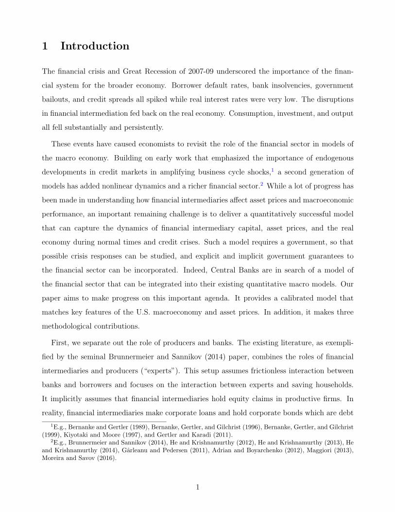
depends on aggregate productivity (ZAt , Zt) and idiosyncratic productivity ωit :

Yi,t = ωi,tZAt K

1−αi,t (ZtLi,t)

α.

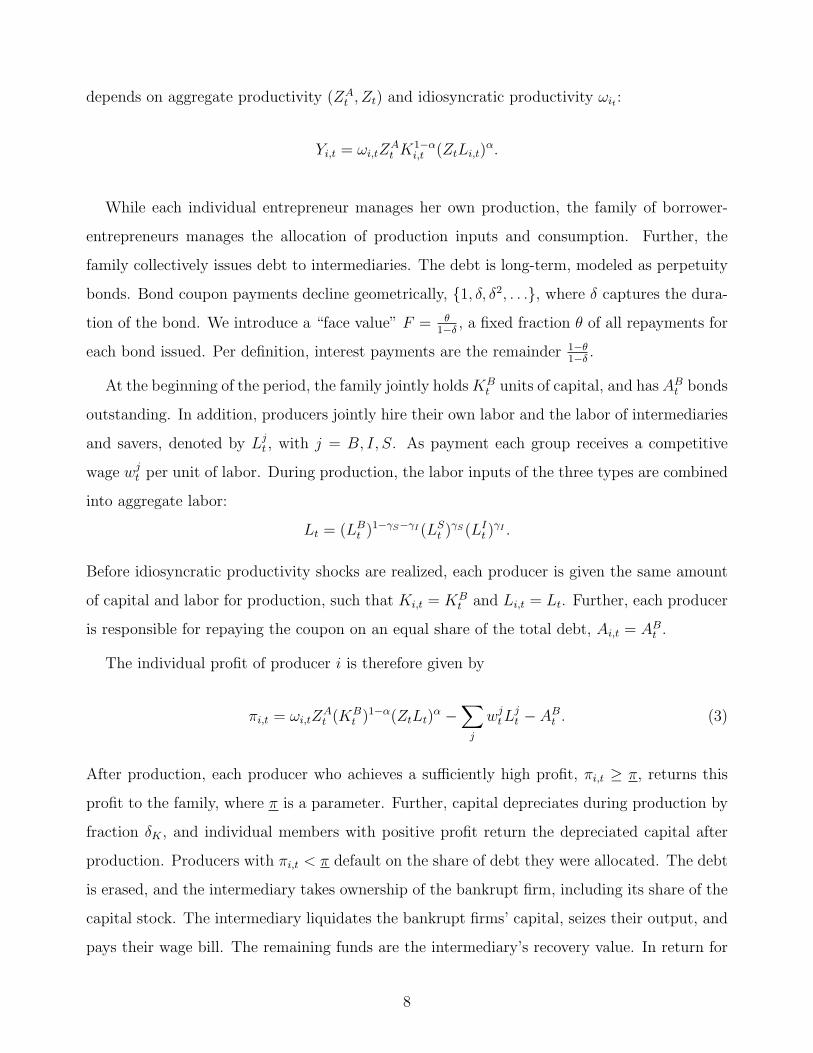
While each individual entrepreneur manages her own production, the family of borrower-

entrepreneurs manages the allocation of production inputs and consumption. Further, the

family collectively issues debt to intermediaries. The debt is long-term, modeled as perpetuity

bonds. Bond coupon payments decline geometrically, 1, δ, δ2, . . ., where δ captures the dura-

tion of the bond. We introduce a “face value” F = θ1−δ

, a fixed fraction θ of all repayments for

each bond issued. Per definition, interest payments are the remainder 1−θ1−δ

.

At the beginning of the period, the family jointly holdsKBt units of capital, and has AB

t bonds

outstanding. In addition, producers jointly hire their own labor and the labor of intermediaries

and savers, denoted by Ljt , with j = B, I, S. As payment each group receives a competitive

wage wjt per unit of labor. During production, the labor inputs of the three types are combined

into aggregate labor:

Lt = (LBt )

1−γS−γI (LSt )

γS(LIt )

γI .

Before idiosyncratic productivity shocks are realized, each producer is given the same amount

of capital and labor for production, such that Ki,t = KBt and Li,t = Lt. Further, each producer

is responsible for repaying the coupon on an equal share of the total debt, Ai,t = ABt .

The individual profit of producer i is therefore given by

πi,t = ωi,tZAt (K

Bt )

1−α(ZtLt)α −

∑j

wjtL

jt − AB

t . (3)

After production, each producer who achieves a sufficiently high profit, πi,t ≥ π, returns this

profit to the family, where π is a parameter. Further, capital depreciates during production by

fraction δK , and individual members with positive profit return the depreciated capital after

production. Producers with πi,t < π default on the share of debt they were allocated. The debt

is erased, and the intermediary takes ownership of the bankrupt firm, including its share of the

capital stock. The intermediary liquidates the bankrupt firms’ capital, seizes their output, and

pays their wage bill. The remaining funds are the intermediary’s recovery value. In return for

8

production, each family member receives the same amount of consumption goods Ci,t = CBt .

From (3), it immediately follows that there exists a cutoff productivity shock

ω∗t =

π +∑

j=B,I,S wjtL

jt + AB

t

ZAt (K

Bt )

1−α(ZtLt)α, (4)

such that all entrepreneurs receiving productivity shocks below this cutoff default on their debt.

Using the threshold level ω∗t , we define ΩA(ω

∗t ) to be the fraction of debt repaid to lenders

and ΩK(ω∗t ) to be the average productivity of the firms that do not default:

ΩA(ω∗t ) = Pr[ωi,t ≥ ω∗

t ], (5)

ΩK(ω∗t ) = Pr[ωi,t ≥ ω∗

t ] E[ωi,t |ωi,t ≥ ω∗t ]. (6)

After making a coupon payment of 1 per unit of remaining outstanding debt, the amount of

outstanding debt declines to δΩA (ω∗t )A

Bt .

The profit of the producers’ business is subject to a corporate profit tax with rate τBΠ . The

profit for tax purposes is defined as sales revenue net of labor expenses, and capital depreciation

and interest payments of non-bankrupt producers:8

ΠB,τt = ΩK(ω

∗t )Z

At (K

Bt )

1−α(ZtLt)α − ΩA(ω

∗t )

(∑j

wjtL

jt + δKptK

Bt + (1− θ)AB

t

).

The fact that interest expenditure ΩA(ω∗t )(1 − θ)AB

t and capital depreciation δKptKBt are de-

ducted from taxable profit creates a “tax shield” and hence a preference for debt funding.

In addition to producing consumption goods, producers jointly create capital goods from

consumption goods. In order to create Xt new capital units, the required input of consumption

goods is

Xt +Ψ(Xt/KBt )K

Bt , (7)

with adjustment cost function Ψ(·) which satisfies Ψ′′(·) > 0, Ψ(µG+δK) = 0, and Ψ′(µG+δK) =

0.

8Aggregate producer profit is the integral over the idiosyncratic profit (3) of non-defaulting producers, netof capital depreciation expenses and adding back principal payments θAB

t which are not tax deductible.

9

The borrower-entrepreneur family’s problem is to choose consumption CBt , capital for next

period KBt+1, new debt AB

t+1, investment Xt and labor inputs Ljt to maximize life-time utility

UBt in (1), subject to the budget constraint:

CBt +Xt +Ψ(Xt/K

Bt )K

Bt + ΩA(ω

∗t )A

Bt (1 + δqmt ) + ptK

Bt+1 + ΩA(ω

∗t )

∑j=B,I,S

wjtL

jt + τBΠΠB,τ

t

≤ ΩK(ω∗t )Z

At (K

Bt )

1−α(ZtLt)α + (1− τBt )wB

t LB + pt(Xt + ΩA(ω

∗t )(1− δK)K

Bt ) + qmt A

Bt+1 +GT,B

t +OBt ,

(8)

and a leverage constraint:

FABt+1 ≤ Φpt(1− (1− τBΠ )δK)ΩA(ω

∗t )K

Bt . (9)

The borrower household uses output, after-tax labor income, sales of old (KBt ) and newly

produced (Xt) capital units, new debt raised (qmt ABt+1), where qmt is the price of one bond

in terms of the consumption good, transfer income from the government (GT,Bt ), and transfer

income from bankruptcy proceedings (OBt ) to be defined below. These resources are used to pay

for consumption, investment including adjustment costs, debt service, new capital purchases,

wages, and corporate taxes.

The borrowing constraint in (9) caps the face value of debt at the end of the period, FABt+1,

to a fraction of the market value of the available capital units after default and depreciation,

pt(1− (1− τBΠ )δK)ΩA(ω∗t )K

Bt , where Φ is the maximum leverage ratio. With such a constraint,

declines in capital prices (in bad times) tighten borrowing constraints. The constraint (9)

imposes a hard upper bound on borrower leverage. In addition, costly defaults of individual

borrowers who received bad idiosyncratic shocks, endogenously limit the optimal leverage of

borrowers. Borrowers take into account that each marginal unit of debt issued in t increases

costly defaults in t+1. Therefore, for a high enough maximum leverage ratio Φ, constraint (9)

will never be binding.

10

2.3 Savers

Savers can invest in one-period risk free bonds (deposits and government debt). They inelasti-

cally supply their unit of labor LS. Entering with wealth W St , the saver’s problem is to choose

consumption CSt and short-term bonds BS

t to maximize life-time utility USt in (1), subject to

the budget constraint:

CSt + qft B

St ≤W S

t + (1− τSt )wSt L

S +GT,St +OS

t (10)

and a short-sale constraints on bond holdings:

BSt ≥ 0. (11)

The budget constraint (10) shows that saver uses after-tax labor income, net transfer income,

and beginning-of-period wealth to pay for consumption, and purchases of short-term bonds

2.4 Intermediaries

After aggregate and idiosyncratic productivity shocks have been realized, financial intermedi-

aries choose whether or not to declare bankruptcy. Intermediaries who declare bankruptcy have

all their assets and liabilities liquidated. They also incur a stochastic utility penalty ρt, with

ρt ∼ Fρ, i.i.d. over time and independent of all other shocks. At the time of the bankruptcy de-

cision, intermediaries do not yet know the realization of the bankruptcy penalty. Rather, they

have to commit to a bankruptcy decision rule D(ρ) : R → 0, 1, that specifies the optimal

decision for every possible realization of ρt. Intermediaries choose D(ρ) to maximize expected

utility at the beginning of the period. We conjecture and later verify that the optimal default

decision is characterized by a threshold level ρ∗t , such that intermediaries default for all realiza-

tions for which the utility cost is below the threshold. The utility penalty is a computational

device to “convexify” the intermediary value function.

After the realization of the penalty, intermediaries execute their bankruptcy choice according

to the decision rule. They then face a consumption and portfolio choice problem to be described

below. First, while intertemporal preferences are still specified by equation (1), intraperiod

11

utility ujt depends on the bankruptcy decision and penalty:

uIt =CI

t

exp (D(ρt)ρt).

Intermediaries’ portfolio choice consists of loans to borrower-entrepreneurs (AIt ) and short-term

bonds (BIt ). Loans are modeled as bonds aggregating the debt of the borrowers. The coupon

payment on performing loans in the current period is AItΩA(ω

∗t ). For borrower-entrepreneurs

that default and enter into foreclosure, the intermediaries repossess their firms, including this

period’s output, as collateral. Intermediaries must pay the wages owed by the defaulting firms,

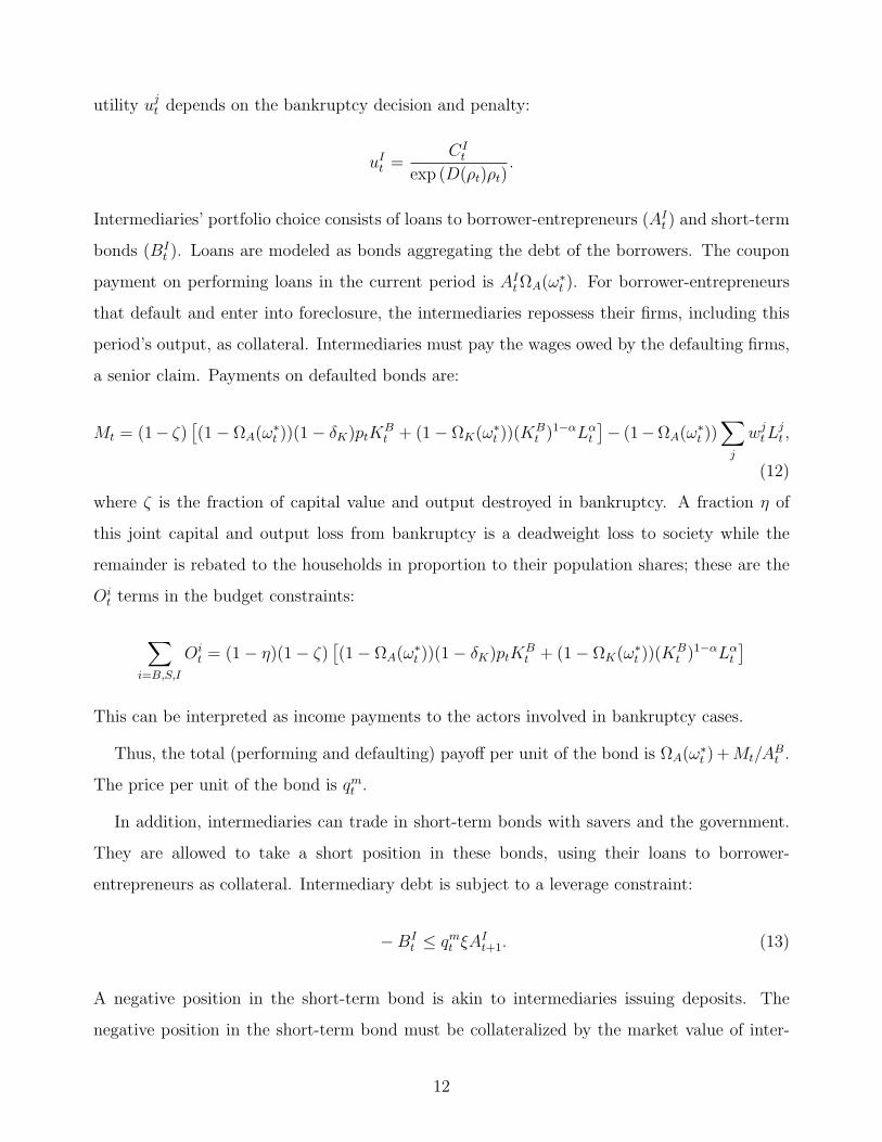
a senior claim. Payments on defaulted bonds are:

Mt = (1− ζ)[(1− ΩA(ω

∗t ))(1− δK)ptK

Bt + (1− ΩK(ω

∗t ))(K

Bt )

1−αLαt

]− (1−ΩA(ω

∗t ))∑j

wjtL

jt ,

(12)

where ζ is the fraction of capital value and output destroyed in bankruptcy. A fraction η of

this joint capital and output loss from bankruptcy is a deadweight loss to society while the

remainder is rebated to the households in proportion to their population shares; these are the

Oit terms in the budget constraints:

∑i=B,S,I

Oit = (1− η)(1− ζ)

[(1− ΩA(ω

∗t ))(1− δK)ptK

Bt + (1− ΩK(ω

∗t ))(K

Bt )

1−αLαt

]This can be interpreted as income payments to the actors involved in bankruptcy cases.

Thus, the total (performing and defaulting) payoff per unit of the bond is ΩA(ω∗t ) +Mt/A

Bt .

The price per unit of the bond is qmt .

In addition, intermediaries can trade in short-term bonds with savers and the government.

They are allowed to take a short position in these bonds, using their loans to borrower-

entrepreneurs as collateral. Intermediary debt is subject to a leverage constraint:

−BIt ≤ qmt ξA

It+1. (13)

A negative position in the short-term bond is akin to intermediaries issuing deposits. The

negative position in the short-term bond must be collateralized by the market value of inter-

12

mediaries’ holdings of long-term loan bonds. The parameter ξ determines how useful loans are

as collateral. The constraint (13) is a Basel-style regulatory capital constraint. The parameter

ξ is the key macro-prudential policy parameter in the paper.

Denote the wealth (net worth) of an intermediary that did not go into bankruptcy by:

W It = ΩA(ω

∗t )(1 + δqmt )A

It +Mt +BI

t−1 (14)

Intermediaries are subject to corporate profit taxes at rate τ IΠ. Their profit for tax purposes

is defined as the net interest income on their loan business:9

ΠIt = (1− θ)ΩA(ω

∗t )A

It + rft B

It−1.

Intermediaries’ also receive after-tax income for supplying their labor to borrower-entrepreneurs,

from government transfers, and from bankruptcy transfers. They further need to pay a deposit

insurance fee (κ) to the government that is proportional to the amount of short-term bonds

they issue. Their budget constraint is:

CIt + qmt A

It+1 + (qft + IBI

t <0κ)BIt + τ IΠΠ

It ≤ (1−D(ρt))W

It + (1− τ I)wI

t LI +GT,I

t +OIt . (15)

Note that intermediaries only receive wealth W It if they do not declare bankruptcy at the

beginning of the period; in case of bankruptcy their wealth is (reset by the government at)

zero.

2.5 Government

The actions of the government are determined via fiscal rules: taxation, spending, bailout, and

debt issuance policies. Government tax revenues, Tt, are labor income tax, corporate profit tax,

and deposit insurance fee receipts:

Tt =∑

j=B,I,S

τ jt wjtL

jt + τBΠΠB

t + τ IΠΠIt − IBI

t <0κBIt

9We define the risk free interest rate as the yield on risk free bonds, rft = 1/qft − 1.

13

Government expenditures, Gt are the sum of exogenous government spending, Got , transfer

spending GTt , and financial sector bailouts:

Gt = Got +

∑j=B,I,S

GT,jt −D(ρt)W

It

The bailout to the financial sector equals the negative of the financial wealth of intermediaries,

W It , in the event of a bankruptcy.

The government issues one-period risk-free debt. Debt repayments and government expen-

ditures are financed by new debt issuance and tax revenues, resulting in the budget constraint:

BGt−1 +Gt ≤ qft B

Gt + Tt (16)

We impose a transversality condition on government debt:

limu→∞

Et

[MS

t,t+uBGt+u

]= 0

where MS is the SDF of the saver.10 Because of its unique ability to tax, the government can

spread out the cost of default waves and financial sector rescue operations over time.

Government policy parameters are Θt =(τ it , τ

iΠ, G

ot , G

T,it , κ,Φ, ξ

). The parameters ϕ in

equation (9) and ξ in equation (13) can be thought of as macro-prudential policy tools. One

could add the parameters that govern the utility cost of bankruptcy of intermediaries to the

set of policy levers, since the government may have some ability to control the fortunes of the

financial sector in the event of a bankruptcy.

2.6 Equilibrium

Given a sequence of aggregate productivity shocks ZAt , idiosyncratic productivity shocks

ωt,ii∈B, and utility costs of default shocks ρt, and given a government policy Θt, a competitive

equilibrium is an allocation CBt , K

Bt+1, Xt, A

Bt+1, L

jt for borrower-entrepreneurs, CS

t , BSt for

10We show below that the risk averse saver is the marginal agent for short-term risk-free debt. In the numericalwork below, we keep the ratio of government debt to GDP contained between bG and bG by decreasing taxeslinearly when the debt-to-GDP threatens to fall below bG and raising taxes linearly when debt-to-GDP threatensto exceed bG.

14

savers, CIt , A

It+1, B

It for intermediaries, bankruptcy rule D(ρt), and a price vector pt, qmt , q

ft ,

such that given the prices, borrower-entrepreneurs, savers, and intermediaries maximize life-

time utility subject to their constraints, the government satisfies its budget constraint, and

markets clear.

The market clearing conditions are:

1. Risk-free bonds:

BGt = BS

t +BIt (17)

2. Loans: ABt+1 = AI

t+1

3. Capital: KBt+1 = (1− δK)K

Bt +Xt

4. Labor: Lit = Lj for all i = B, I, S

5. Consumption:

Yt =(CBt + CI

t + CSt ) +Go

t +Xt +KBt Ψ(Xt/K

Bt )︸ ︷︷ ︸

INV

+ ηζ[(1− ΩA(ω

∗t ))(1− δK)ptK

Bt + (1− ΩK(ω

∗t ))(K

Bt )

1−αLαt

]︸ ︷︷ ︸DWL

The last equation is the economy’s resource constraint. It states that total output (GDP) equals

the sum of aggregate consumption, discretionary government spending, and investment (INV),

and deadweight costs (DWL) incurred when liquidating bankrupt firms, a fraction ηζ of the

capital and output of defaulting firms.

2.7 Welfare

In order to compare economies that differ in the policy parameter vector Θt, we must take a

stance on how to weigh the different agents. We propose a utilitarian social welfare function

summing value functions of the agents

Wt(·; Θt) = V Bt + V S

t + V It ,

15

where the V j(·) functions are the value functions defined in the appendix. The value functions

already incorporate the mass of agents of each type (population shares ℓi).11

2.8 Model without Intermediation Sector

We also consider a simplified version of the model without intermediaries. We refer to this

version as the “consolidated balance sheet” (CBS) model, since it involves merging borrowers

and intermediaries into one group of agents, which for simplicity we still call borrowers. In

the CBS model, borrowers can directly issue risk-free deposits to savers.12 Instead of issuing

defaultable corporate loans to intermediaries, they now choose holdings BBt of risk-free debt

subject to the budget constraint:

CBt +Xt +Ψ(Xt/K

Bt )K

Bt + (qft + IBB

t <0κ)BBt + ptK

Bt+1 +

∑j=B,I,S

wjtL

jt + τBΠΠB,τ

t

≤ ZAt (K

Bt )

1−α(ZtLt)α + (1− τBt )wB

t LB +BB

t−1 + pt(Xt + (1− δK)KBt ) +GT,B

t +OBt ,

(18)

and are subject to the leverage constraint:

−BBt ≤ Ξpt(1− (1− τBΠ )δK)K

Bt ,

where parameter Ξ limits the amount of risk-free debt borrowers can issue. We redefine corpo-

rate profits as

ΠB,τt = ZA

t (KBt )

1−α(ZtLt)α −

(∑j

wjtL

jt + δKptK

Bt

)+ rft B

Bt−1

to reflect the different tax shield. An important difference with the benchmark is that credit

frictions associated with corporate debt, and therefore the cross-sectional productivity shocks

11Equivalently, we could first express the value functions per capita by scaling them by their populationweights, and then calculating a population-weighted average of the per capita value functions.

12Given the difference in patience, borrowers will issue debt to savers. We assume that this debt is insured bythe government in the same fashion as the intermediaries’ debt in the benchmark version of the model. However,for realistic levels of corporate leverage (< 50%), aggregate government bailouts will play no role in the CBSmodel.

16

ωi,t, are no longer relevant in the CBS model.

3 Calibration

The model is calibrated at annual frequency. The parameters of the model and their targets

are summarized in Table 1.

Aggregate Productivity Labor-augmenting productivity grows at a deterministic rate of

µG equal to 2.0% per year, in order to match observed average GDP growth of 2.0% per year.

Following the macro-economics literature, the TFP process ZAt follows an AR(1) in logs with

persistence parameter ρA and innovation volatility σA. Because TFP is persistent, it becomes

a state variable. We discretize gt into a 5-state Markov chain using the Rouwenhorst (1995)

method. The procedure chooses the productivity grid points and the transition probabili-

ties between them to match the volatility and persistence of HP-detrended GDP. The latter

is endogenously determined but heavily influenced by TFP. Consistent with the model, our

measurement of GDP excludes net exports, housing investment, changes in inventories, and

government investment. We define the GDP deflator correspondingly. Observed real per capita

HP-detrended GDP has a volatility of 2.13% and its persistence is 0.68. The model generates

a volatility of 2.24% and a persistence of 0.76.

Idiosyncratic Productivity We calibrate the firm-level productivity risk directly to the

micro evidence. We normalize the mean of idiosyncratic productivity at µω = 1. We let

the cross-sectional standard deviation of idiosyncratic productivity shocks σt,ω follow a 2-state

Markov chain. Fluctuations in σt,ω are the second source of aggregate risk. Fluctuations in σt,ω

govern aggregate corporate credit risk since high levels of σt,ω cause a larger left tail of low-

productivity firms that default. We refer to states with the high value for σt,ω as high uncertainty

periods. We set (σL,ω, σH,ω) = (0.095, 0.175). The value for σL,ω targets the unconditional mean

corporate default rate. The model-implied average default rate of 2.4% is similar to the data.13

13We look at two sources of data: corporate loans and corporate bonds. From the Flow of Funds, we obtaindelinquency and charge-off rates on Commercial and Industrial loans and Commercial Real Estate loans by U.S.Commercial Banks for the period 1991-2015. The average delinquency rate is 3.1%. The second source of datais Standard & Poors’ default rates on publicly-rated corporate bonds for 1981-2014. The average default rate

17

Table 1: Calibration

Par Description Value Target

Exogenous Shocks

µG mean growth 2.0% Mean rpc GDP gr 53-14 of 2.00%

ρA persistence TFP 0.65 AC(1) HP-detr GDP 53-14 of 0.68

σA innov. vol. TFP 1.9% Vol HP-detr GDP 53-14 of 2.13%

σω,L low uncertainty 0.095 Avg. corporate default rate

σω,H high uncertainty 0.175 Avg. IQR firm-level productivity

pωLL, pωHH transition prob 0.91, 0.80 Bloom et al. (2012)

Production, Population, Labor Income Shares

ψ marginal adjustment cost 2 Vol. investment-to-GDP ratio 53-14 of 1.23%

α labor share in prod. fct. 0.71 Labor share of output of 2/3

δK capital depreciation rate 10% Justiniano, Primiceri, and Tambalotti (2010)

ℓi pop. shares i ∈ S,B, I 69,28.3,2.7% Population shares SCF 95-13, QCEW 01-15

γi inc. shares i ∈ S,B, I 60,37.4,2.6% Labor inc. shares SCF 95-13, QCEW 01-15

Corporate loans

δ average life loan pool 0.937 Duration fcn. in App. B.1

θ principal fraction 0.582 Duration fcn. in App. B.1

ζ Losses in bankruptcy 0.5 Corporate loan and bond severities 81-15

η % bankr. loss is DWL 0.2 Bris, Welch, and Zhu (2006)

Φ maximum LTV ratio 0.45 Vol. of risk free rate 85-14

π profit default threshold 0.04 FoF non-fin sector leverage 85-14

Preferences

βB = βI time discount factor B, I 0.95 FoF fin sector leverage 85-14 of 90%

σ risk aversion B, I, S 1 Log utility

ν IES B, I, S 1 Relative volatility of aggr. cons and GDP

βS time discount factor S 0.995 Mean risk-free rate 85-14

Government Policy

Go discr. spending 17.17% BEA discr. spending to GDP 53-14 of 17.58%

GT transfer spending 2.42% BEA transfer spending to GDP 53-14 of 3.18%

τ labor income tax rate 28.0% BEA pers. tax rev. to GDP 53-14 of 17.30%

τΠ corporate tax rate 21.7% BEA corp. tax rev. to GDP 53-14 of 3.41%

bo cyclicality discr. spending -2.9 slope log discr. sp./GDP on GDP growth

bT cyclicality transfer spending -27 slope log transfer sp./GDP on GDP growth

bτ cyclicality lab. inc. tax 2.6 slope log discr. sp./GDP on GDP growth

κ deposit insurance fee 0 Deposit insurance fee 97-06

ξ max. intermediary leverage 0.95 Basel II reg. capital charge for C&I loans

σρ utility cost bankruptcy 10% Technical assumption

18

The high value, σH,ω, is chosen to match the time-series standard deviation of the cross-

sectional interquartile range of firm productivity, which is 4.9% according to Bloom, Floetotto,

Jaimovich, Saporta-Eksten, and Terry (2012) (their Table 6).

The transition probabilities from the low to the high uncertainty state of 9% and from the

high to the low state of 20% are also taken directly from Bloom et al. (2012).14 The model

spends 31% of periods in the high uncertainty regime. Like in Bloom et al., our uncertainty

process is independent of the first-moment shocks. About 10% of periods feature both high

uncertainty and low TFP realizations. We will refer to those periods as financial recessions or

financial crises. Using a long time series for the U.S., Reinhart and Rogoff (2009) find a similar

10% frequency of financial crises.

Production Adjustment costs are quadratic. We set the marginal adjustment cost parameter

ψ = 2 in order to match the observed volatility of the ratio of investment to GDP, X/Y , of

1.23%. The model generates a value of 1.19%. The adjustment costs are a tiny 0.04% of GDP

in the steady state. We set the parameter α in the Cobb-Douglas production function equal to

0.71, which yields an overall labor income share of 66.5%, the standard value in the business

cycle literature. We choose δK to match an annual depreciation of capital of 10%, a typical

value used for example in Justiniano, Primiceri, and Tambalotti (2010).

Population and Labor Income Shares To pin down the population shares of our three

different types of households we turn to the Survey of Consumer Finance (SCF). We define

savers as those households who hold a low share of their wealth in the form of risky assets. In

particular, we compute for each household in the survey the share of assets, net of all real estate,

held in stocks or private business equity, considering both direct and indirect holdings of stock.

Using this definition of the risky share, we then calculate the fraction of households whose risky

share is less than one percent.15 This amounts to 69% of SCF households. The remaining 31%

of households have a large risky asset share. We split them into 28.3% borrowers-entrepreneurs

is 1.5%; 0.1% on investment-grade bonds and 4.1% on high-yield bonds. The model is in between these twovalues.

14They estimate a two-state Markov chain for the cross-sectional standard deviation of establishment-levelproductivity using annual data for 1972-2010 from the Census of Manufactures and Annual Survey of Manufac-tures. We annualize their quarterly transition probability matrix.

15We use all survey waves from 1995 until 2013 and average across them.

19

and 2.7% financial intermediaries based on the share of employees that work in the financial

sector, defined as “Securities, Investments” and “Credit Intermediation” from the Quarterly

Census of Employment and Wages (QCEW), averaged over the longest available sample 2001-

2015.

From the same QCEW data, we obtain the wage share for the intermediaries of 2.6%. The

labor income share of savers in the SCF is 60%. The income share of the borrower-entrepreneurs

is the remaining 37.4%. The income shares determine the Cobb-Douglas parameters γI , γB,

and γS. By virtue of the calibration, the model matches basic aspects of the observed income

distribution. It also matches the size of the U.S. intermediary sector.16

Corporate Loans In the model, a corporate loan is a geometric bond. The issuer of one

bond at time t promises to pay 1 at time t + 1, δ at time t + 2, δ2 at time t + 3, and so on.

Given that the present value of all payments (1/(1 − δ)) can be thought of as the sum of a

principal (share θ) and an interest component (share 1 − θ), we define the book value of the

debt as F = θ/(1− δ). This book value of debt is used in the firm’s collateral constraint. We

set δ = 0.937 and θ = 0.582 (F = 9.238) to match the observed duration of corporate bonds.

Appendix B.1 contains the details. The model’s corporate loans have a duration of 7 years on

average.

As in standard trade-off theory, corporate debt enjoys a tax shield but incurs costs of distress.

We set the ζ = 0.5 to match the observed average severity rate of 44% on bonds rated by S&P

and Moody’s rated during 1985-2004. The model produces a similar unconditional loss-given

default of 42%. Combined with the average default rate, this LGD number implies a loss rate on

corporate loans of 1.1%. Our baseline model generates a modest quantity of corporate default

risk, consistent with the data.

A fraction η of the cost of distress to intermediaries is a deadweight loss to the economy.

The remainder 1− η is transfer income that enters in the budget constraint of the agents. We

set η = 0.2 based on evidence in Bris, Welch, and Zhu (2006). The resulting deadweight losses

16Intermediaries’ labor income is 2.6% of total labor income and 1.73% of GDP pre-tax and 1.25% after-tax.After-tax profits are an additional 2.07% of GDP. Total after-tax intermediary income is 3.32% of GDP in themodel. The market value of intermediated assets is 84.6% of GDP. Thus, intermediary income is 3.92% ofintermediated assets. Intermediary profits are 2.45% of intermediated assets. Philippon (2015) reports that thecost of financial intermediation has historically been about 2% of intermediated assets.

20

of default average to 0.54% of GDP in the benchmark model.

Borrowers can obtain a loan with principal value up to a fraction Φ of the market value of

their assets. We set the maximum LTV ratio parameter Φ = 0.45. This value is just large

enough so that the LTV constraint never binds during expansions (it rarely binds during non-

financial recessions). In the simulation of our benchmark model, the borrower’s LTV constraint

binds in 20% of financial recessions. The LTV constraint limits corporate borrowing as a

fraction of the market value of capital. We found that the presence of the capital price (Tobin’s

q) in the infrequently binding constraint is one of the main amplification mechanisms of the

model, causing sharper financial recessions when firms become constrained. The volatility of

the risk free rate is a direct indicator of the severity of these episodes in our model, since risk

free rates fall sharply during financial recessions. The model produces a risk free rate volatility

of 2.34%, in line with data estimates.17 We note that the volatility of the real interest rate is

only 1.1% in the model if we exclude the financial recessions.

We set the profit default threshold to π = 0.04 to target non-financial leverage. The higher

this threshold, the more firms will default on average for a given level of firm debt. Since defaults

are costly to the borrower family, borrower leverage is decreasing in π. The model generates a

ratio of borrower book debt-to-assets of 42%. In the Flow of Funds data, the average ratio of

loans and debt securities of the nonfinancial corporate and nonfinancial noncorporate businesses

to their non-financial assets is 37%, a slightly lower value.18

Preference Parameters Preference parameters affect many equilibrium quantities and prices

simultaneously, and are harder to pin down directly by data. In order to highlight the separate

roles of intermediaries’ and firms’ balance sheets, we purposely set the time discount factor

and the risk aversion coefficient of borrowers and intermediaries equal. We assume that all

households have log utility: σ = ν = 1. We set the EIS ν = 1 in order to approximately

match the relative volatility of aggregate consumption to that of output. The model currently

produces consumption volatility that is slightly lower than in the data. Since a higher EIS leads

17To calculate the real rate, we take the nominal one year constant maturity Treasury yield (FRED) andsubtract expected inflation over the next 12 months from the Survey of Professional Forecasters for the sample1985-2014.

18For the Flow of Funds leverage data, we use the post-1987 sample. Only in this sample is nonfinancialleverage stationary. Our model certainly misses some reasons for firms to hold more cash (negative debt) suchas international tax reasons.

21

to consumption that is more volatile relative to output, we could use a higher EIS to match

this volatility; however, for simplicity, we use log utility.

The subjective time discount factors βB = βI = 0.95 target financial sector leverage. The

average ratio of total intermediary debt-to-assets for 1985-2014 is 90.7%.19 The model generates

average intermediary debt-to-asset ratio of 91.5% (debt evaluated at book value, assets at

market value).

The time discount factor of the saver disproportionately affects the mean of the short-term

interest rate. We set βS = 0.995 to generate a low average real rate of interest of 2.65%.

Government Parameters To add quantitative realism to the model, we match both the

unconditional average and the cyclical properties of discretionary spending, transfer spending,

labor income tax revenue, and corporate income tax revenue.

Discretionary and transfer spending as a fraction of GDP are modeled as follows: Git/Yt =

Gi exp bi(gt − g) , i = o, T . The scalars Go and GT are set to match the observed average

discretionary spending to GDP of 17.58% in the 1953-2014 NIPA data, and transfer spending

to GDP of 3.18%, respectively.20 We set bo = −2.9 and bT = −27 in order to match the slope

in a regression of log spending to GDP on GDP growth and a constant. We match these slopes:

-0.81 and -7.57 in the model versus -0.75 and -7.26 in the 1953-2014 data.

Similarly, we model the labor income tax rate as τt = τ exp bτ (gt − g). We set the tax

rate τ = 28.0% in order to match observed average income tax revenue to GDP of 17.3%.21

19Krishnamurthy and Vissing-Jorgensen (2015) identify a group of financial institutions as net suppliers ofsafe, liquid assets. This group contains U.S. Chartered Commercial Banks and Savings Institutions, ForeignBanking offices in U.S., Bank Holding Companies, Banks in U.S. Affiliated Areas, Credit Unions, FinanceCompanies, Security Brokers and Dealers, Funding Corporations, Money market mutual funds, GSEs, Agency-and GSE-backed mortgage pools, Issuers of ABS, and REITs. The group of excluded financial institutions areInsurance Companies, other Mutual Funds, Closed-end funds and ETFs, and State, Local, Federal, and PrivatePension Funds.

20We divide by expbi/2σ

2g/(1− ρ2g)(bi − 1)

, a Jensen correction, ensure that average spending means match

the targets.21We define income tax revenue as current personal tax receipts (line 3) plus current taxes on production and

imports (line 4) minus the net subsidies to government sponsored enterprises (line 30 minus line 19) minus thenet government spending to the rest of the world (line 25 + line 26 + line 29 - line 6 - line 9 - line 18). Our logicfor adding the last three items to personal tax receipts is as follows. Taxes on production and export mostlyconsist of federal excise and state and local sales taxes, which are mostly paid by consumers. Net governmentspending on GSEs consists mostly of housing subsidies received by households which can be treated equivalentlyas lowering the taxes that households pay. Finally, in the data, some of the domestic GDP is sent abroad in theform of net government expenditures to the rest of the world rather than being consumed domestically. Since

22

The model generates an average of 18.3%. We set the sensitivity of the tax rate to aggregate

productivity growth bτ = 2.6 to match the observed sensitivity of log income tax revenue to

GDP to GDP growth. The regression slope of log income tax revenue to GDP on GDP growth

and a constant produces similar pro-cyclicality: 0.98 in the model and 0.70 in the data.

Fourth, we set the corporate tax rate that both financial and non-financial corporations pay

to a constant τΠ = 21.7% to match observed corporate tax revenues of 3.41% of GDP. The

model generates an average of 3.01%. The tax shield of debt and depreciation that firms and

banks enjoy in the model substantially reduces the effective tax rate they pay.

The final source of government spending is interest service on the debt, which is endogenous

since both quantity and price of government debt are determined in equilibrium. In the data, net

interest payments on government debt average to 2.98% of GDP.22 This number is close to the

observed average budget deficit of 3.04% of GDP. We do not aim to match this number since

the government cannot run a 3% deficit in perpetuity in the model, lest the debt explodes.

In our calibration, the personal and corporate tax revenue is very close to the discretionary

and transfer spending; the primary surplus averages 0.5% of GDP. Government debt to GDP

averages 55.6% of GDP in a long simulation of the benchmark model. While it fluctuates

meaningfully over prolonged periods of time (standard deviation of 46.6%), the government

debt to GDP ratio remains stationary.23

Macro-prudential Policy We can interpret the intermediary borrowing constraint param-

eters, ξ, as a regulatory capital constraint set by the government. Under Basel II and III,

corporate loans and bonds have a risk weight that depends on their credit quality. For a 40%

loss given default, the risk weight on commercial and industrial bank loans with 2.5 year ma-

the model has no foreigners, we reduce personal taxes for this amount, essentially rebating this lost consumptionback to domestic agents.

22Net interest expenses are interest payments to persons and businesses (line 28) minus income receipts onasses (line 10).

23In our numerical work, we guarantee the stationarity of the ratio of government debt to GDP by graduallydecreasing personal tax rates τt when debt-to-GDP falls below bG = 0.1 –the profligacy region– and by graduallyincreasing personal tax rates when debt-to-GDP exceed bG = 1.2 –the austerity region. Specifically, taxes aregradually and smoothly lowered with a convex function until they hit zero at debt to GDP of -0.1. Tax ratesare gradually and convexly increased until they hit 60% at a debt-to-GDP ratio of 150%. Our simulations neverreach the -10% and +150% debt/GDP states. The simulation spends 25% of the time in the profligacy and13% of the time in the austerity region. The fraction of time spent in these regions has no effect on the overallresources of the economy.

23

turity ranges from 13% for AAA, 54% for BBB-, 125% for B+, to 325% for CCC. A blended

regulatory capital requirement of 5% (8% times a blended risk weight of 62.5%) seems appro-

priate. This implies that ξ = 0.95. This is the key parameter we vary in or macro-prudential

policy experiments.

We set the deposit insurance fee parameter κ = 0 to reflect the fact that banks were not

required to pay any deposit insurance fees between 1997 and 2006.24 We will explore the

alternative value of κ = 0.25%.

Utility cost of intermediary bankruptcy The model features a random utility penalty

that intermediaries suffer when they default. Because random default is mostly a technical

assumption, it is sufficient to have a small penalty at least some of the time. We assume ρt is

normally distributed with a mean of µρ =1, i.e., a zero utility penalty on average, and a small

standard deviation of σρ = 0.10. The standard deviation of the penalty affects the correlation

between negative intermediary wealth and intermediary defaults. The frequency of government

bailouts of intermediaries depends on the frequency of credit crises and the endogenous (asset

and liability) choices of the intermediaries.

4 Results

Before discussing the main results on macro-prudential policy, we study the behavior of key

macro-economic and financial variables. They capture important features of the data and lend

credibility to the policy experiments that are to follow. Specifically, we report means and

standard deviations from a long simulation of the model (10,000 years), as well as averages

conditional on being in a good state (positive TFP growth and low uncertainty, i.e. σω,L), non-

financial recession (negative TFP growth, low uncertainty), and financial recession (negative

TFP growth and high uncertainty σω,H).

24FDIC premia were raised after the crisis. Well capitalized banks currently pay 2.5 cents per $100 insured.

24

Table 2: Unconditional Macroeconomic Quantity Moments

Data Model

stdev output corr. AC stdev output corr. AC

GDP 2.13% 1.00 0.68 2.24% 1.00 0.76CONS 1.87% 0.91 0.65 1.52% 0.9 0.73X/Y 1.23% 0.19 0.87 1.19% 0.41 0.36X/K 0.89% 0.44 0.82 0.75% 0.46 0.30

4.1 Macro Quantities

Table 2 reports the standard deviation of aggregate quantities, their correlation with GDP, and

their autocorrelation. Moments in the data are computed from HP-detrended series. Moments

in the model are deterministically detrended since all time series have a deterministic trend.

The model matches the volatility of GDP and aggregate consumption. It also matches the

autocorrelation of both series. The model matches the volatility of the investment to GDP

ratio (1.19% vs. 1.23%) by virtue of the adjustment cost parameter choice, and delivers an

investment rate volatility that approximates the data (0.75% vs. 0.89%). The investment/GDP

ratio and investment rate display modest pro-cyclicality in both data and model. Investment

rates are insufficiently persistent in the model.25 As discussed in the calibration section, the

model also matches the cyclicality of government spending.

We present impulse-response graphs to explore the behavior of macro-economic quantities

conditional on the state of the economy. We start off the model in year 0 in the average TFP

state (the middle of the five points on the TFP grid) and in the low uncertainty state (σω,L).

In period 1, the model undergoes a change to the lowest-TFP grid point. In one case (red

line), the recession is accompanied by a switch to the high uncertainty state (σω,H); a financial

recession. In the second case, the economy remains in the low uncertainty state; a non-financial

recession (blue line). From period 2 onwards, the two exogenous state variables follow their

stochastic laws of motion. For comparison, we also show a series that does not undergo any

shock in period 1 but where the exogenous states stochastically mean revert from the high-TFP

state in period 0 (black line). For each of the three scenarios, we simulate 10,000 sample paths

of 25 years and average across them. Figure 2 plots the macro-economic quantities, detrended

25As an aside, the investment level is too smooth (1.15% volatility in the model vs. 6.31% in the data) whileinvestment growth is too volatile (10.94% vs. 6.14% in the data).

25

by their long-term growth rate of 2% per year. The top left panel is for the productivity level

Z. By construction, it falls by the same amount in financial and non-financial recessions; a 2%

drop. Productivity then gradually mean reverts over the next decade. The black line shows

how productivity would have evolved absent a shock in period 1.

Figure 2: Financial vs. Non-financial Recessions: Macro Quantities

0 5 10 15 20 250.98

0.985

0.99

0.995

1

1.005TFP

0 5 10 15 20 250.965

0.97

0.975

0.98

0.985

0.99Output

0 5 10 15 20 250.55

0.56

0.57

0.58

0.59

0.6Consumption

0 5 10 15 20 250.17

0.18

0.19

0.2

0.21

0.22

0.23

0.24Investment

The graphs show the average path of the economy through a recession episode which starts at time 1. In period0, the economy is in the average TFP state. The recession is either accompanied by high uncertainty (highσω), a financial recession plotted in red, or low uncertainty (low σω), a non-financial recession) plotted in blue.From period 2 onwards, the economy evolves according to its regular probability laws. The black line plots thedynamics of the economy absent any shock in period 1. We obtain the three lines via a Monte Carlo simulationof 10,000 paths of 25 periods, and averaging across these paths. Blue line: non-financial recession, Red line:financial recession, Black line: no shocks.

The other three panels show impulse-responses for GDP, consumption, and investment. The

percentage drop in GDP is larger than that in productivity and the drop in GDP is larger

when the economy is additionally hit by an uncertainty shock (red line) than if it is not (blue

line). In financial recessions, the economy suffers from a second period of decline, despite the

26

rebound in productivity. GDP remains lower for longer in a financial recession. The added

persistence resembles the slow recovery that typically follows a financial crisis. The bottom

right panel shows a 30% drop in investment in financial recessions but only a modest drop

in non-financial recessions. The investment rate dynamics track Tobin’s q (our variable p) by

virtue of the first-order condition for firm investment. Despite the bounce back in period 2,

investment remains depressed for a prolonged period of time. Aggregate consumption offsets

the initial decline in investment in a financial recession. The low rate of return on savings

induces the saver to consume more in a financial crisis. Consumption drops subsequently and

remains below the non-financial recession level for the remaining periods.

4.2 Balance Sheet Variables

Next, we turn to the key balance sheet variables in Table 3. The first two columns report

the unconditional mean and volatility. The last three columns report conditional averages in

expansions, non-financial recessions, and financial recessions, respectively.

Firms The first panel focuses on the borrower-entrepreneurs, the non-financial corporate

sector. Rows 1 and 2 display the market value of assets (ptKBt ) and the market value of

liabilities (qmt ABt ), both scaled by GDP. Their difference is the market value of firm equity

scaled by GDP. Their ratio is the market leverage ratio (row 4). Book leverage, defined as the

book value of debt to the book value of assets in row 3, is 43%. Entrepreneurs own more than

half of their firms in the form of corporate equity (57%). Market leverage is counter-cyclical

while book leverage is pro-cyclical. Firms delever in financial recessions, hence the fall in book

leverage, but sharp drops in the market value of assets lead to an increase in market leverage.

Indeed, Tobin’s q (the variable p in row 16) falls by 3.27% on average from expansions to

financial recessions, although this average masks a substantially larger initial drop.

Individual borrowers default when their profits are too low. This is more likely when the

cross-sectional distribution of idiosyncratic productivity shocks widens, as the mass of firms with

productivity shocks below the threshold ω∗t increases. The model generates average corporate

default and loss rates of 2.85% (row 7) and 1.29% points (row 9), respectively, implying an

average loss-given-default rate of 45.4% (row 8). All these numbers are in line with the data.

27

Default and loss rates are higher in financial recessions (6.6% and 2.97%) than in non-financial

recessions and expansions (about 1.1% and 0.5% in both). The model generates the right

amount of corporate credit risk, on average, and generates the strong cyclicality in the quantity

of risk observed in the data.26

Most of the time, firms stay away from the leverage constraint because they are risk averse

and take into account the costs of bankruptcy when making their leverage choices. However,

borrowers are likely to be constrained in financial recessions (18% of the time, row 6). This

occurs because of the fall in the price of collateral. When the constraint binds, firms are forced

to cut their borrowing from the financial sector, and cannot pursue the investment projects

they would otherwise undertake. Relative to expansions, output falls by 3.8% and investment

by 28% in financial recessions, in part due to these binding constraints.

Intermediaries Intermediary market leverage is 93% on average (row 11 of Table 3), match-

ing the data. Intermediaries choose to be so highly levered for a number of reasons. Like the

corporate firms, they are impatient and enjoy a tax shield. As the only agent with access to

deposits, they alone can earn a large spread (2.03%, row 19) between the short-term deposit

rate (2.59%, row 17) and the rate on corporate loans (4.62%, row 18). They bear the interest

rate risk associated with the maturity transformation they perform, as well as the credit risk

on the loans. Given the low (but realistically calibrated) average loss rate and their relatively

low risk aversion, they choose to take up substantial leverage to reach their desired risk-return

combination.

Adrian, Boyarchenko, and Shin (2015) show that book leverage is pro-cyclical while mar-

ket leverage is counter-cyclical both for commercial banks and for broker-dealers. Our model

generates this pattern. Market leverage increases from 92.8% in expansions to 93.84% in non-

financial recessions, and to 93.19% in financial recessions. Book leverage, in contrast, falls

from 92.47% in expansions to 88.79% in financial recessions. Why does market leverage rise in

financial recessions? Intermediaries suffer losses on their credit portfolio. The realized excess

return on bank assets is -0.08% (row 20). At the same time risk is high and low prices (high

26In the 1991 recession, the delinquency rate spiked at 8.2% and the charge-off rate at 2.2%. For the 2007-09crisis, the respective numbers are 6.8% and 2.7%. These are far above the unconditional averages of 3.1% and0.7% cited in footnote 13. Similarly, during the 2001 recession, the default rate on high-yield bonds was 9.9%,far above the 1981-2014 average of 4.1%.

28

Table 3: Balance Sheet Variables and Prices

Unconditional Expansions Non-fin Rec. Fin Rec.

mean stdev mean mean mean

Borrower

1. Mkt Val of Capital / Y 1.966 0.038 1.989 1.986 1.9202. Mkt Val of Corp Debt / Y 0.828 0.035 0.848 0.824 0.7873. Book val corp debt / Y 0.843 0.021 0.851 0.848 0.8254. Market corp leverage 42.88% 0.86% 42.81% 42.68% 42.98%5. Book corp leverage 42.87% 0.72% 43.23% 42.40% 42.03%6. Fraction leverage constr binds 4.83% 21.44% 0.13% 1.81% 18.21%7. Default rate 2.85% 2.55% 1.10% 1.15% 6.69%8. Loss-given-default rate 45.42% 2.13% 46.02% 44.66% 44.19%9. Loss Rate 1.29% 1.17% 0.51% 0.51% 2.97%

Intermediary

10. Mkt fin leverage 93.19% 2.36% 92.81% 93.84% 93.19%11. Book fin leverage 91.47% 1.88% 92.47% 91.17% 88.79%12. Fraction leverage constr binds 32.21% 46.73% 0.02% 45.91% 75.52%13. Bankruptcies 0.00% 0.00% 0.00% 0.00% 0.00%

Saver

14. Deposits / Y 0.771 0.031 0.787 0.773 0.73215. Government Debt / Y 0.879 0.421 0.862 1.013 0.871

Prices

16. Tobin’s q 1.000 0.015 1.010 0.994 0.97817. Risk-free rate 2.59% 2.34% 3.42% 3.90% 0.25%18. Corporate bond rate 4.62% 0.26% 4.46% 4.73% 4.93%19. Credit spread 2.03% 2.27% 1.04% 0.83% 4.68%20. Excess return on corp. bonds 0.79% 1.78% 1.34% 0.39% -0.08%

29

yields, row 18) of corporate bonds and loans reflect the higher default risk and the higher credit

risk premium. This reduces the market value of intermediary assets. A lower value of bank as-

sets tightens their regulatory capital constraint. The intermediary leverage constraint binds in

75.5% of the financial crises compared to 32.2% unconditionally. When binding, intermediaries

must reduce liabilities to meet capital requirements in the wake of their credit losses. Given

the low cost of deposit funding in a financial crises (0.25%) and the high credit spreads they

earn in those states of the world (4.68%), intermediaries would like to raise more deposits and

increase corporate lending but their constraint prevents them from doing so.

In sharp contrast, intermediaries are only constrained in 46% of the non-financial recessions.

The risk free rate rises in such period, to 3.9%, as all agents want to borrow against future

income to smooth consumption. At the same time, demand for credit is low due to worse

investment opportunities, and the credit spread shrinks. Intermediaries are hardly ever con-

strained during expansions (.02%). In those periods, investment opportunities are good and

intermediaries expand both lending and deposits, while earning their desired rate of return.

The size of the intermediary sector, relative to GDP, shrinks in financial recessions. Both

book and market values of intermediary assets shrink about 8% relative to their levels in

expansions (rows 2 and 3). At the same time that the value of bank assets shrinks, their

liabilities shrink (row 14). Bank liabilities fall from 79% of GDP in expansions to 73% of GDP

in financial recessions (row 15). Since GDP itself falls, bank liabilities themselves fall by as

much as 12%.

Intermediary net worth, or bank equity, is an important state variable in all intermediary-

based models. Intermediary net worth is the difference between the market value of bank assets

(row 2) and the value of deposits (row 15). Intermediary equity is 5.67% of GDP unconditionally.

It shrinks to 5.4% of GDP in the average financial recession. The reduction in intermediary

net worth itself is 15.8%, relative to the unconditional level. The reduction in net worth in

financial crises makes intermediaries effectively more risk averse, leading them to charge larger

risk premia on new lending. We return to this risk premium effect below. Low net worth

hampers the intermediaries’ capacity to bear credit risk and do maturity transformation.

In the equilibrium of our model, the intermediation sector as a whole is never insolvent.

Even in the absence of systemic intermediary failures in equilibrium, deposit insurance lowers

30

the cost of funding and provides banks with a risk shifting motive vis-a-vis the government.

However, as risk averse agents, bank owners are reluctant to hit low net worth states since they

imply low consumption and high marginal utility. The balance of these two factors determines

the frequency of financial breakdowns.27.

Figure 3: Financial vs. Non-financial Recessions: Balance Sheet Variables Intermediaries

0 5 10 15 20 251.86

1.87

1.88

1.89

1.9

1.91

1.92Book value of corp assets

0 5 10 15 20 250.79

0.8

0.81

0.82

0.83

0.84Book value of corp liabilities

0 5 10 15 20 250.95

0.96

0.97

0.98

0.99

1

1.01Price of capital

0 5 10 15 20 250.98

1

1.02

1.04

1.06

1.08

1.1

1.12Market value of corp equity

0 5 10 15 20 250.005

0.01

0.015

0.02

0.025

0.03

0.035

0.04Loss rate

0 5 10 15 20 250

0.01

0.02

0.03

0.04

0.05

0.06

0.07

0.08Loan spread

0 5 10 15 20 250.71

0.72

0.73

0.74

0.75

0.76

0.77Book value of fin liabilities

0 5 10 15 20 250.055

0.06

0.065

0.07

0.075

0.08

0.085Market value of fin equity

Blue line: non-financial recession, Red line: financial recession, Black line: no shocks.

Figure 3 show the impulse-response functions for assets and liabilities of both non-financial

firms and banks. The top row reports book values of corporate assets (capital) and liabilities

(loans). Corporations shrink ob both sides of their balance sheet during financial recessions.

The market value of corporate equity, with both assets and liabilities valued at market prices,

drops sharply in financial recessions due to the sharp drop in Tobin’s q (top row, right hand

side). The book value of corporate liabilities is also the book value of financial assets. In the

27Whether or not systemic failures occur depends on both the magnitude of shocks, and the strength of therisk shifting motive. See for example Elenev, Landvoigt, and Van Nieuwerburgh (2016) for a model with afinancial intermediary that can choose to hold riskier assets.

31

third graph on the bottom row, we can see that banks’ liabilities (book value) fall by even more

than their assets during financial recession; simply put, banks delever during these periods.

Because of large losses on their loan portfolio (bottom row, first graphs), banks need to charge

large credit spreads (bottom row, second graph). This reduces the demand for loans. Even

though financial book leverage declines, market leverage increases in crises, or equivalently, the

market value of financial equity declines (bottom row, fourth graph). This is because the market

value of liabilities rises more sharply than the market value of assets. Banks slowly rebuild their

equity capital (through high spreads and low intermediary household consumption) and expand

their loans business as loss rates return to normal levels. In the simulation, this process takes

close to 20 years.

Savers Risk averse savers only hold safe debt, provided both by the intermediaries and the

government. On average, these two sources of safe assets account for 77% (row 14) and 87% of

GDP (row 15). In our model, as in the data, the government’s tax revenues are pro-cyclical and

its expenses counter-cyclical. However, the small expansion in government debt to GDP more is

not enough to offset the reduction in deposits so that the total equilibrium supply of safe short-

term assets falls in financial recessions. As a result, the equilibrium real interest rate falls 300

basis points from expansions to financial recessions. In financial recessions, intermediaries want

to delever due to their equity losses. This delevering requires savers to increase consumption

and reduce savings exactly at a time when their marginal utility of consumption is high. To

induce savers to dissave, a large drop in the real interest rate is required. The magnitude of this

drop depends on savers’ EIS, everything else equal. If savers’ EIS is high, they are more willing

to increase consumption in crises, and the interest will fall by less. This will shift the cost of

crises onto borrowers and intermediaries, who cannot profit from negative real interest rates. If

savers’ EIS is low, real interest rates become negative and help to recapitalize intermediaries.28

Prices Real interest rates on safe debt are 2.59% on average and have a volatility of 2.34%

(row 17). Both are very reasonable numbers, especially in a production-based asset pricing

28For example, when νS = 60 >> 1, the risk-free interest rate volatility approaches zero. Intermediaries nolonger benefit from low, even negative interest rates in crises. The absence of cheap funding in crises makesthem more reluctant to take on more leverage in the first case. This very high saver EIS world is akin to thecontinuous time intermediation model of Brunnermeier and Sannikov where risk-free rates are constant. Theeconomy with low EIS behaves quite differently.

32

model, and match historical averages. Financial recessions see large declines in collateral values

(row 16), negative (excess) returns on bank assets (row 20), high corporate credit spreads (row

19), and low real interest rates (row 17). All of these are important features of real-life financial

crises. In contrast, non-financial recessions see only modest reductions in risk-free rates and

modest increases in credit spreads.

One important quantitative success of the model is its ability to generate a high unconditional

credit spread while matching the observed amount of default risk. The average 2.03% spread is

close to the average 2.39% spread in the data.29 The credit spread is also highly volatile (2.27%

standard deviation) and strongly counter-cyclical (four times higher in financial recessions than

expansions). The rise in the credit spread in financial recessions to 4.68% reflects not only the

increase in the default risk but also an increase in the credit risk premium. The model generates

a high and counter-cyclical price of credit risk, which itself comes from the high and counter-

cyclical SDF of the intermediary, who is the marginal agent in the corporate loan market. The

sharp decline in intermediary wealth is responsible for the sharp increase in the SDF.

Figure 4 shows the impulse-responses in the bust experiment for the interest rates, the credit

spread, and the price of capital. In the first period of a financial recession following a boom,

the real risk-free rate turns sharply negative and the credit spread blows out to 8%. Financial

recessions are periods of high credit risk and credit risk premia, both of which enter in the

credit spread. For reasons explained above, the risk free rate plummets to -3.5%. Non-financial

recessions see a much smaller risk-free rate and credit spread effect, and a much smaller decline

in the price of capital.

29We define the credit spread as the difference between the yield on a blended portfolio of investment gradeand high yield bonds and the yield on a one-year constant maturity Treasury yield. We use the longest availablesample from Barclays U.S. corporate IG and HY bond indices from February 1987 to December 2015. Todetermine the portfolio weights on the high yield versus investment grade bonds, we use market values of theamounts outstanding, also from Barclays. The average weight on HY is 19.4%. The resulting credit spread hasa mean of 3.36% and a volatility of 1.46%. We compare this with a difference measure of the credit spread whichtakes a 19.4%-80.6% weighted average of the Moody’s Aaa and Baa yields and subtracts the one-year CMTrate. Over the same February 1987-December 2015 period, the mean credit spread is 3.05% with a volatilityof 1.39%. The second measure of the credit spread has a correlation of 86% with the first one. The advantageof this second measure is that we can compute it back to 1953. The mean spread over the 1953-2015 period is2.08% with a volatility of 1.55%. While the second credit spread is downward biased, compared to the betterfirst measure, considering a longer sample period would lead us to consider a lower mean credit spread targetthan 3.36%. For example, we could add the 31 basis point difference between our favorite Barclays measure andthe Moody’s measure over the post-1987 sample to the full-sample Moody’s mean of 2.08% to get to a targetmean credit spread for the full 1953-2015 sample of 2.39%.

33

Figure 4: Financial vs. Non-financial Recessions: Prices

0 5 10 15 20 25-0.04

-0.03

-0.02

-0.01

0

0.01

0.02

0.03

0.04Riskfree rate

0 5 10 15 20 250.044

0.045

0.046

0.047

0.048

0.049Loan rate

0 5 10 15 20 250

0.01

0.02

0.03

0.04

0.05

0.06

0.07

0.08Loan spread

0 5 10 15 20 250.95

0.96

0.97

0.98

0.99

1

1.01Capital price

Blue line: non-financial recession Red line: financial recession.

4.3 Consumption and Welfare

Table 4 reports the moments of consumption for each agent, as well as each agent’s value func-

tion, and aggregate welfare. By virtue of being the largest groups of agents, borrowers and

savers have the highest consumption shares (relative to GDP). More interesting is consumption

growth in the second panel. It reveals that the intermediary has by far the most volatile con-

sumption growth (13%), followed by the saver (3.5%), and the borrower (2.4%). We recall that

borrowers and intermediaries have the identical preferences (risk aversion, patience, and IES),

so that these differences in consumption volatility arise endogenously from the different roles

they perform in the economy (production vs. intermediation). Intermediaries end up absorbing

a disproportionate fraction of the aggregate risk in the economy. In financial recessions, all

three agents suffer drops in their consumption, but the drop is far larger for intermediaries

34

Table 4: Consumption and Welfare

Unconditional Expansions Non-fin Rec. Fin Rec.mean stdev mean mean mean

Consumption to Output

Consumption, B 0.229 0.007 0.234 0.226 0.219Consumption, I 0.018 0.003 0.020 0.017 0.014Consumption, S 0.329 0.013 0.329 0.315 0.326

Consumption growth

Consumption, B 2.00% 2.40% 2.69% 1.58% 0.42%Consumption, I 2.00% 13.08% 5.36% 0.77% -6.56%Consumption, S 2.00% 3.53% 2.16% 0.62% 1.24%

Welfare

Aggregate welfare 17.573 0.030 17.583 17.567 17.550Value function, B 0.3367 0.0034 0.3381 0.3351 0.3340Value function, I 0.0254 0.0007 0.0259 0.0253 0.0246Value function, S 17.211 0.032 17.219 17.207 17.191DWL/GDP 0.008 0.007 0.003 0.003 0.018

Marginal utility ratios

log(MU B / MU I) 0.014 0.128 0.082 0.008 -0.134log(MU B / MU S) -1.272 0.048 -1.288 -1.305 -1.238log(MU S / MU I) 1.286 0.142 1.370 1.312 1.104

(-26%) than for borrowers (-6.7%) or savers (-0.8%).

The third panel reports moments related to aggregate welfare. Overall welfare, the popula-

tion weighted average of the three agents’ value functions measured in consumption equivalent

units, is highest in expansions and lowest in financial recessions. Given the large difference in

discount factors, aggregate welfare calculations are dominated by savers. The welfare differ-

ence between expansions and financial recessions for savers and therefore aggregate welfare is

small at 0.2%. However, intermediaries have 5.5% lower welfare in financial recessions than in

expansions, while borrowers have 1.2% lower welfare.

The last panel reports ratios of marginal utilities between pairs of agents. In a complete

markets model with agents whose preference parameters differ, these ratios would differ across

pairs of agents but be constant over time. Our model is an incomplete markets model featuring

imperfect risk sharing; the marginal utility ratios display high volatility between 5% and 14%.

For example, the marginal utility of borrower and intermediary are nearly equalized on average,

but the borrower has 8% higher marginal utility than the intermediary in expansions and 13%

lower marginal utility in financial recessions.

35

4.4 Credit Spread and Risk Premium

Figure 5 shows the histogram of the intermediary wealth share plotted against three different

measures of credit risk compensation earned by intermediaries. The solid red line plots the

credit spread, the difference between the yield rmt on corporate bonds and the risk-free rate,

where we compute the bond yield as rmt = log(

1qmt

+ δ).30 Consistent with the result in He

and Krishnamurty (2013), the credit spread is high when the financial intermediary’s wealth

share is low. Since our model has defaultable debt, the increase in the credit spread reflects

both risk-neutral compensation for expected defaults and a credit risk premium.

To shed further light on the source of the high credit spread, we compute the expected excess

return (EER) on corporate loans/bonds earned by the intermediary. The EER consists both of

the credit risk premium, defined as the (negative) covariance of the intermediary’s stochastic

discount factor with the corporate bond’s excess return, and an additional component that

reflects the tightness of the intermediary’s leverage constraint. This component arises because

the marginal agent in the market for risk-free debt is the saver household, while corporate

bonds are priced by the constrained intermediary. The market risk free rate is lower than the

“shadow” risk free rate implied by intermediary consumption smoothing. To decompose the

expected excess return into the risk premium and constraint tightness components, we plot both

the complete EER on corporate bonds (the dashed red line) and the risk premium (the dotted

red line). When the intermediary wealth share is relatively high, the leverage constraint is not

binding and the EER is equal to the risk premium, which is approximately zero in this region

of the state space. Low levels of intermediary wealth result from credit losses, and the lowest

levels occur during financial crises. At these times, credit risk increases and the intermediary

becomes constrained. In the worst crisis when intermediary wealth gets close to zero, the EER

reaches 3 percent. The conventional risk premium (the covariance of intermediary SDF and

bonds return) accounts for 1 percentage points of the EER.

30This is a simple way of transforming the price of the long-term bond into a yield; however, note that thisdefinition assumes a default-free payment stream (1, δ, δ2, . . .) occurring in the future.

36

Figure 5: The Credit Spread and the Financial Intermediary Wealth Share

0.01 0.015 0.02 0.025 0.03 0.035 0.04 0.045 0.05

Intermediary wealth share

-0.01

0

0.01

0.02

0.03

0.04

0.05C

redi

t Spr

ead

and

Exp

ecte

d E

xces

s R

etur

n

0

0.05

0.1

0.15

0.2

0.25

Freq

uenc

y

Solid line: credit spread; dashed line: expected excess return; dotted line: risk premium (covariance betweenintermediary SDF and corporate bond excess return). The difference between expected excess return and riskpremium is a measure for tightness of the intermediary constraint.

4.5 Effect of Decoupling Firm and Intermediary Balance Sheets

We solve the CBS version of the model, described in section 2.8, to understand how the disag-

gregation of firm and intermediary balance sheets affects macroeconomic dynamics. We keep

all model parameters the same as in the benchmark model. All parameters of intermediation

sector and the parameters related to corporate credit frictions are no longer relevant. Since

firms directly issue risk-free debt to savers, there is no more corporate default, and the idiosyn-

cratic productivity shocks of firms wash out in the aggregate. This also means that there are

no DWL from costly liquidations in the CBS model. We set the parameter governing maximum

firm leverage, Ξ, to 0.49, such that the deposit-to-GDP ratio is equal to the benchmark model

(87%). Table 5 compares prices and quantities of the CBS model to the benchmark.

Two clear effects emerge from the comparison: the CBS economy is significantly smaller,

but also much less volatile. In the CBS model, Tobin’s q is 36.5% less volatile (row 2), and this

37

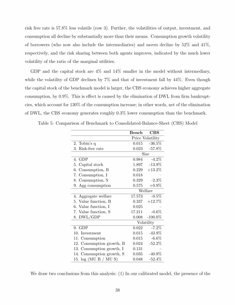
risk free rate is 57.8% less volatile (row 3). Further, the volatilities of output, investment, and

consumption all decline by substantially more than their means. Consumption growth volatility

of borrowers (who now also include the intermediaries) and savers decline by 52% and 41%,

respectively, and the risk sharing between both agents improves, indicated by the much lower

volatility of the ratio of the marginal utilities.

GDP and the capital stock are 4% and 14% smaller in the model without intermediary,

while the volatility of GDP declines by 7% and that of investment fall by 44%. Even though

the capital stock of the benchmark model is larger, the CBS economy achieves higher aggregate

consumption, by 0.9%. This is effect is caused by the elimination of DWL from firm bankrupt-

cies, which account for 130% of the consumption increase; in other words, net of the elimination

of DWL, the CBS economy generates roughly 0.3% lower consumption than the benchmark.

Table 5: Comparison of Benchmark to Consolidated-Balance-Sheet (CBS) Model

Bench CBS

Price Volatility

2. Tobin’s q 0.015 -36.5%3. Risk-free rate 0.023 -57.8%

Size

4. GDP 0.984 -4.2%5. Capital stock 1.897 -13.9%6. Consumption, B 0.229 +13.2%7. Consumption, I 0.018 –8. Consumption, S 0.329 -2.3%9. Agg consumption 0.575 +0.9%

Welfare

4. Aggregate welfare 17.573 -0.5%5. Value function, B 0.337 +12.7%6. Value function, I 0.025 –7. Value function, S 17.211 -0.6%8. DWL/GDP 0.008 -100.0%

Volatility

9. GDP 0.022 -7.2%10. Investment 0.015 -43.9%11. Consumption 0.015 -6.6%12. Consumption growth, B 0.024 -52.2%13. Consumption growth, I 0.131 –14. Consumption growth, S 0.035 -40.9%15. log (MU B / MU S) 0.048 -52.4%

We draw two conclusions from this analysis: (1) In our calibrated model, the presence of the

38

separate intermediation sector is critical for capturing the volatility of macroeconomic prices and

quantities observed in the data. The CBS model with the same fundamental productivity risk

is not able to generate large financial recessions, even though a standard financial accelerator

effect is present in firms’ leverage constraint. (2) The additional volatility and risk caused

by the intermediation sector in the benchmark model leads to greater precautionary savings

motives, and higher wealth accumulation by borrowers (capital) and savers (risk free debt). In

general equilibrium, this effect may lead to higher output and consumption.

5 Macro-prudential Policy

We use our calibrated model to investigate the effects of macro-prudential policy choices. Our

main experiment is a variation in the intermediaries’ leverage constraint. In the benchmark

model, intermediaries can borrow 95 cents against every dollar in assets (ξ = 0.95). We explore

tighter constraints (ξ = .70, ξ = 0.80, ξ = 0.90), as well as looser constraints (ξ = .975). Our

second macro-prudential policy experiment is to charge intermediaries κ = 0.025% for deposit

insurance, about the present-day level. Tables 6 and 7 show the results. Table 7 reports results

in percentage deviation from the benchmark.

Changing maximum intermediary leverage Rows 10 and 11 of Table 6 show that a

policy that constrains bank leverage is indeed successful at bringing down that leverage. Banks

reduce the size of their assets, both in book and market value terms (rows 2 and 3) and

the size of their liabilities (row 14). On net, intermediary equity increases sharply as ξ is

lowered. With intermediaries better capitalized, financial fragility falls. With tighter regulation,

intermediaries’ constraints bind more frequently (row 12). As the economy becomes less risky,

intermediaries can be less cautious and exhaust the borrowing capacity more frequently. In

sum, tighter regulation leads to a safer intermediary sector, but also to a smaller one.

This increased safety is also reflected in lower corporate default, loss-given-default, and loss

rates for non-financial firms as ξ falls (rows 7-9). Firms choose to reduce leverage (rows 4-5)

and their LTV constraints rarely bind (row 6). Firms reluctance to undertake more leverage

despite the safer environment may be understood from the higher interest rates and spreads

39

Table 6: Macroprudential Policy

Benchmark ξ = .70 ξ = .80 ξ = .90 ξ = .975 κ = 0.25%

Borrowers

1. Mkt value capital/GDP 1.966 1.924 1.950 1.958 1.970 1.9572. Mkt value corp debt/GDP 0.828 0.606 0.741 0.808 0.835 0.8063. Book val corp debt/GDP 0.843 0.649 0.785 0.835 0.846 0.8354. Market corp leverage 0.429 0.337 0.402 0.426 0.429 0.4265. Book corp leverage 0.429 0.337 0.402 0.426 0.429 0.4266. Fraction LTV constr binds 4.83% 0.00% 0.13% 3.16% 5.26% 2.91%7. Default rate 2.85% 1.89% 2.48% 2.79% 2.87% 2.79%8. Loss-given-default rate 45.42% 29.63% 40.25% 44.57% 45.66% 44.48%9. Loss Rate 1.29% 0.53% 0.98% 1.24% 1.31% 1.23%

Intermediaries

10. Mkt fin leverage 0.932 0.690 0.793 0.886 0.951 0.93611. Book fin leverage 0.915 0.644 0.749 0.857 0.938 0.90412. Fraction intermed constr binds 32.21% 90.56% 79.22% 46.71% 22.78% 37.92%

Savers

13. Deposits/GDP 0.771 0.418 0.588 0.716 0.794 0.75414. Government debt/GDP 0.879 0.631 0.731 0.836 0.883 0.655

Prices

15. Tobin’s q 1.000 1.000 1.000 1.000 1.000 1.00016. Risk-free rate 2.59% 2.60% 2.56% 2.59% 2.59% 2.58%17. Corporate bond rate 4.62% 5.16% 5.04% 4.78% 4.56% 4.79%18. Credit spread 2.03% 2.56% 2.47% 2.19% 1.97% 2.22%19. Excess return on corp. bonds 0.79% 2.11% 1.55% 1.00% 0.71% 1.03%

they face on debt (rows 18 and 19). When intermediary capacity shrinks (with lower ξ), the

reward for providing intermediation services increases. Higher financial sector profitability is

evidenced by a higher credit spread in the face of lower loss loan rates.

The smaller banking sector reduces the supply of deposits (row 14). Further, lower non-

financial and financial leverage mean that firms and banks take less advantage of their tax shield

of debt, increasing government tax revenues and reducing government debt (row 15). The overall

reduced supply of safe assets would depress equilibrium interest rates at constant demand. Why

then do rates stay roughly constant as ξ is tightened (row 17)? As the economy becomes less

volatile, so does saver consumption growth. This reduces saver demand for precautionary

savings, offsetting the drop in supply of risk free debt.

Because of the higher profit margin, the intermediary’s consumption is higher (row 30 of Ta-

ble 7). Intermediaries not only experience higher consumption, their consumption also becomes

less volatile (row 36). Naturally then, intermediary welfare increases with tighter constraints

40

(row 23). Interestingly (or ironically), it is the agent whose constraint is tightened that benefits

the most from the policy change. Intermediaries in the benchmark model could have chosen a

much lower leverage ratio. They did not since they did not internalize the positive effect that

lower sector-wide intermediary leverage would have had on credit spreads.

The savers’ welfare is adversely affected by tighter bank capital regulation (row 24). Their

wealth, which is wholly invested in risk free debt, declines substantially, while the return (the

risk free rate) stays roughly constant. Hence their consumption falls. Given their large size in

the population (69%) and the large weight they receive in aggregate welfare due to their high

discount rate, the effect on savers is important for understanding the overall negative welfare

effect form tighter macro-prudential policy.

Borrowers’ consumption rises weakly (row 29), and their consumption volatility declines

(row 36). Therefore, like intermediaries, they are better off from large declines in intermediary

leverage (row 22). Risk sharing improves substantially when financial leverage is lower, as

witnessed by the reduced volatility in the marginal utility ratios across pairs of agents (rows

39-41).

A first key effect of macro-prudential policies is that they reduce macro-economic volatility.

The last panel of Table 7 indeed shows reductions in GDP growth, investment growth, and

consumption growth volatility (rows 32, 34, 35).

A second key effect of tighter macro-prudential policy is that the economy’s output shrinks

(row 26). The capital stock shrinks sizeably (row 27). The reduction in output arises be-

cause firms choose to borrow less from a smaller intermediary sector. Debt financing becomes

significantly more expensive, eliminating a previously cheap source of financing.

The aggregate welfare effect of tighter bank capital requirements is modest (row 21). Tighter

bank capital requirements reduce the risk in the economy but they shrink the total pie. On net,

we find that tighter macro-prudential policy has modest welfare losses, on the order of 52-244

basis points consumption equivalent loss, depending on the extent of tightening. Conversely,

loosening bank leverage constraints to ξ = .975 would increase welfare by 26 basis points.

Increasing cost of deposit insurance The last column of Tables 6 and 7 show the result of

an experiment that increases the cost of deposit insurance κ from 0 to 0.25% per unit of deposit.

41

Table 7: Macroprudential Policy: Macro and Welfare

Benchmark ξ = .70 ξ = .80 ξ = .90 ξ = .975 κ = 0.25%

Welfare

21. Aggregate welfare 17.573 -2.44% -1.54% -0.52% +0.26% -0.04%22. Value function, B 0.337 +2.22% +0.55% +0.02% +0.00% +0.49%23. Value function, I 0.025 +33.81% +26.03% +8.96% -3.71% -1.07%24. Value function, S 17.211 -2.59% -1.63% -0.55% +0.27% -0.05%25. DWL/GDP 0.008 -35.00% -13.64% -2.43% +0.84% -2.48%

Size of the Economy

26. GDP 0.984 -0.88% -0.33% -0.17% +0.08% -0.2%27. Capital stock 1.897 -3.00% -1.13% -0.60% +0.28% -0.6%28. Aggr. Consumption 0.575 +0.4% +0.2% +0.0% -0.0% +0.0%29. Consumption, B 0.231 +3.0% +0.8% +0.0% +0.0% +0.5%30. Consumption, I 0.022 +31.2% +24.0% +7.7% -2.4% -1.3%31. Consumption, S 0.333 -3.0% -1.5% -0.4% +0.1% -0.2%

Volatilies

32. GDP 2.24% -4.26% -1.77% -0.59% +0.32% -1.3%33. Risk-free rate 2.34% -61.8% -47.2% -23.6% +6.9% -28.2%34. Investment 1.48% -37.6% -19.7% -7.5% +2.0% -11.1%35. Consumption 1.52% -5.7% -7.5% -3.8% +1.1% -3.0%36. Consumption, B 0.68% -5.1% -2.1% -1.5% +1.4% -5.2%37. Consumption, I 0.28% -48.9% -42.7% -21.8% +12.9% -7.5%38. Consumption, S 1.30% -21.3% -13.7% -6.4% +1.1% -5.5%39. log (MU B / MU S) 0.048 -30.3% -13.4% -7.0% +1.2% -7.8%40. log (MU S / MU I) 0.141 -71.4% -55.0% -26.7% +14.2% -3.0%41. log (MU B / MU I) 0.128 -73.8% -71.0% -35.7% +17.7% -9.7%

Column benchmark are moments from a 10,000 period simulation of the benchmark economy. Othercolumns are percentage changes of these moments relative to the benchmark level in a 10,000 periodsimulation of the economies with the parameter change indicated by the column header.

This experiment reduces welfare by 4 basis points. Borrowers gain from this experiment, while

the other two agents lose. Again, capital and GDP fall, but so does GDP and consumption

volatility. The net effect is a redistribution from intermediaries and savers, who bear the

“incidence” of the insurance fee, to borrowers.

6 Conclusion

We provide the first calibrated macro-economic model which features intermediaries who extend

long-term defaultable loans to firms producing output and raise deposits from risk averse savers,

and in which both banks and firms can default. The model incorporates a rich set of fiscal policy

rules, including deposit insurance, and endogenizes the risk-free interest rate.

42

Like in the standard accelerator model, shocks to the macro-economy affect entrepreneurial

net worth. Since firm borrowing is constrained by net worth, macro-economic shocks are

amplified by tighter borrowing constraints. Unlike the original models, ours features impatient

but risk averse and infinitely-lived entrepreneurs. A second financial accelerator arises from

explicitly modeling the financial intermediaries’ balance sheet as separate from that of the

entrepreneur-borrowers and saving households. Intermediaries are subject to regulatory capital

constraints. Macro-economic shocks that lead to binding intermediary borrowing constraints

amplify the shocks through their direct effect on intermediaries’ net worth and the indirect

effect on borrowers to whom the intermediaries lend. However, when intermediaries are well

enough capitalized to absorb the fundamental shock without constraining the firms, they can

dampen the first accelerator mechanism.

We explore the dynamics of quantities and prices in this setting and compare them to U.S.

data, with a focus on understanding differences between financial and non-financial recessions.

Our main application studies macro-prudential policy and contrasts restrictions on firm leverage

to those on bank leverage. While such policies reduce the credit risk and promote macro-

economic stability and better risk sharing among the agents, they potentially shrink the size of

the economy and may ultimately be welfare-reducing.

Extensions to this model could introduce New Keyenesian elements such as nominal rigidities,

monopolistic competition, and monetary policy. Our setting is an interesting one to evaluate the

effect of the zero lower bound (ZLB) on nominal short rates. A binding ZLB during a financial

crisis would keep the real rate elevated. The ZLB economy would prevent the intermediaries

from recapitalizing in a crisis through a negative real deposit rate. Negative real rates mitigate

the severity of financial recessions in the current model. The upshot is that a binding ZLB may

lead to a severe crisis exactly because it prevents a recapitalization of financial intermediaries.

References

Adrian, T., and N. Boyarchenko (2012): “Intermediary leverage cycles and financial

stability,” Working paper.

43

Adrian, T., N. Boyarchenko, and H. Shin (2015): “The Cyclicality of Leverage,” Federal

Reserve Bank of New York Staff Reports No. 743.

Bernanke, B. S., and M. Gertler (1989): “Agency Costs, Net Worth and Business Cycle

Flutuations,” American Economic Review, 79, 14–31.

Bernanke, B. S., M. Gertler, and S. Gilchrist (1996): “The Financial Accelerator and

the Flight to Quality,” The Review of Economics and Statistics, 78(1), 1–15.

(1999): “The financial accelerator in a quantitative business cycle framework,” in

Handbook of Macroeconomics, ed. by J. B. Taylor, and M. Woodford, vol. 1 of Handbook of

Macroeconomics, chap. 21, pp. 1341–1393. Elsevier.

Bianchi, J., and E. Mendoza (2013): “Optimal Time-consistent Macroprudential Policy,”

NBER Working paper 19704.

(2015): “Phases of Global Liquidity, Fundamentals News, and the Design of Macro-

prudential Policy,” Working paper BIS No 505.

Bloom, N., M. Floetotto, N. Jaimovich, I. Saporta-Eksten, and S. J. Terry

(2012): “Really uncertain business cycles,” NBER Working Paper No 18245.

Bris, A., I. Welch, and N. Zhu (2006): “The Costs of Bankruptcy: Chapter 7 Liquidation

versus Chapter 11 Reorganization,” The Journal of Finance, 61(3), 1253–1303.

Brunnermeier, M. K., and Y. Sannikov (2014): “A macroeconomic model with a financial

sector,” The American Economic Review, 104(2), 379–421.

Chen, H. (2010): “Macroeconomic Conditions and the Puzzles of Credit Spreads and Capital

Structure,” Journal of Finance, 65(6), 2171–2212.

Dang, T. V., G. Gorton, and B. Holmstrom (2015): “The Information Sensitivity of a

Security,” .

Elenev, V. (2017): “Mortgage Credit, Aggregate Demand, and Unconventional Monetary

Policy,” .

44

Elenev, V., T. Landvoigt, and S. Van Nieuwerburgh (2016): “Phasing out the GSEs,”

Journal of Monetary Economics, 81(C), 111–132.

Farhi, E., and J. Tirole (2012): “Collective moral hazard, maturity mismatch, and systemic

bailouts,” Americcan Economic Review, pp. 60–93.

Farhi, E., and I. Werning (2016): “A Theory of Macroprudential Policies in the Presence

of Nominal Rigidities,” Econometrica, 84(5), 1645–1704.

Garleanu, N., and L. H. Pedersen (2011): “Margin-based Asset Pricing and Deviations

from the Law of One Price,” Review of Financial Studies.

Gertler, M., and P. Karadi (2011): “A model of unconventional monetary policy,” Journal

of Monetary Economics, 58(1), 17–34.

Guerrieri, L., and M. Iacoviello (2015): “Occbin: A Toolkit to Solve Models with Oc-

casionally Binding Constraints Easily,” Journal of Monetary Economics, 70, 22–38.

Guerrieri, V., and G. Lorenzoni (2015): “Credit Crises, Precautionary Savings, and the

Liquidity Trap,” Working Paper University of Chicago and Northwestern University.

Hansen, G. D. (1985): “Indivisible Labor and the Business Cycle,” Journal of Monetary

Economics, 16, 309–327.

He, Z., and A. Krishnamurthy (2012): “A Model of Capital and Crises,” The Review of

Economic Studies, 79(2), 735–777.

He, Z., and A. Krishnamurthy (2013): “Intermediary asset pricing,” American Economic

Review, 103 (2), 732–770.

(2014): “A Macroeconomic Framework for Quantifying Systematic Risk,” Working

Paper University of Chicago and Stanford University.

Jorda, O., M. Schularick, and A. Taylor (2014): “Betting the House,” NBER Working

Paper No. 20771.

Judd, K. L. (1998): Numerical Methods in Economics, MIT Press Books. The MIT Press.

45

Judd, K. L., F. Kubler, and K. Schmedders (2002): “A solution method for incomplete

asset markets with heterogeneous agents,” Working Paper, SSRN.

Justiniano, A., G. Primiceri, and A. Tambalotti (2010): “Investment Shocks and

Business Cycles,” Journal of Monetary Economics, 57(2), 132–145.

Kiyotaki, N., and J. Moore (1997): “Credit Cycles,” Journal of Political Economy, 105(2),

211–48.

Korinek, A. (2012): “Systemic Risk-Taking: Amplification Effects, Externalities, and Regu-

latory Responses,” Working paper University of Maryland.

Krishnamurthy, A., and A. Vissing-Jorgensen (2015): “The Impact of Financial Supply

on Financial Sector Lending and Stability,” Journal of Financial Economics, 118(2), 571–600.

Kubler, F., and K. Schmedders (2003): “Stationary Equilibria in Asset-Pricing Models

with Incomplete Markets and Collateral,” Econometrica, 71(6), 1767–1793.

Lorenzoni, G. (2008): “Inefficient Credit Booms,” Review of Economic Studies, 75, 809–833.

Maggiori, M. (2013): “Financial intermediation, international risk sharing, and reserve cur-

rencies,” Working paper.

Mendoza, E. (2010): “Sudden Stops, Financial Crises, and Leverage,” American Economic

Review, 100, 1941–1966.

Moreira, A., and A. Savov (2016): “The macroeconomics of shadow banking,” The Journal

of Finance.

Philippon, T. (2015): “Has the US Finance Industry Become Less Efficient?,” American

Economic Review, 105, 1408–1438.

Reinhart, C. M., and K. Rogoff (2009): This time is different: Eight centuries of financial

folly. Princeton University Press.

Rouwenhorst, G. (1995): “Asset Pricing Implications of Equilibrium Business Cycle Mod-

els,” in Frontiers of Business Cycle Research, ed. by Cooley. Princeton University Press.

46

A Model Appendix

A.1 Borrower-entrepreneur problem

A.1.1 Technology

The exogenous laws of motion for labor-augmenting productivity Zt and the TFP level ZAt are

respectively (lower case letters denote logs):

logZt = logZt−1 + g

logZAt = (1− ρA)z

A + ρA logZAt−1 + ϵAt ϵAt ∼ iidN (0, σA)

Denote µG = eg, and µZA = ezA+

(σA)2

2(1−ρ2A

) .

Idiosyncratic productivity of borrower-entrepreneur i at date t is denoted

ωi,t ∼ iidN (µω, σ2ω,t),

and individual output isYi,t = ωi,tZ

At K

1−αt (ZtLt)

α.

Aggregate production is

Yt =

∫Ω

Yi,tdF (ωi) =

∫Ω

ωdF (ω)ZAt K

1−αt (ZtLt)

α = µωZAt K

1−αt (ZtLt)

α.

Individual producer profit is

πi,t = Yi,t −∑j

wjLj − At.

Therefore, the default cutoff at πi,t = π is

ω∗t =

π +∑

j wjtL

jt + At

Yt/µω

.

A.1.2 Preliminaries

We start by defining some preliminaries.

ΩA(ω∗t ) = 1− Fω,t(ω

∗t )

ΩK(ω∗t ) =

∫ ∞

ω∗t

ωdFω,t(ω) = (1− Fω,t(ω∗t ))µω + σω,tϕ

(ω∗t − µω

σω,t

)

47

where Fω,t(·) is the CDF of ωi,t with parameters (µω, σ2ω,t), and where ϕ() is the pdf of a standard

normal random variable.

It is useful to compute the derivatives of ΩK(·) and ΩA(·):

∂ΩK(ω∗t )

∂ω∗t

=∂

∂ω∗t

∫ ∞

ω∗t

ωfω(ω)dω = −ω∗t fω(ω

∗t ),

∂ΩA(ω∗t )

∂ω∗t

=∂

∂ω∗t

∫ ∞

ω∗t

fω(ω)dω = −fω(ω∗t ),

where fω(·) is the p.d.f. of a normal distribution with parameters (µω, σ2ω).

Capital Adjustment Cost Let

Ψ(Xt, KBt ) =

ψ

2

(Xt

KBt

− (µG + δK)

)2

KBt .

Then partial derivatives are

ΨX(Xt, KBt ) = ψ

(Xt

KBt

− (µG + δK)

)(19)

ΨK(Xt, KBt ) = − ψ

2

((Xt

KBt

)2

− (µG + δK)2

)(20)

A.1.3 Optimization Problem

We consider the producers’s problem in the current period after aggregate TFP and idiosyn-cratic productivity shocks have been realized, after the intermediary has chosen a default policy,and after the intermediary’s random utility penalty is realized. To ensure stationarity of theproducer’s problem we define the following transformed variables,

CBt , Xt, A

Bt , K

Bt , w

jt , G

T,Bt

,

where for any variable ˆvart denotes division by the current realization of (deterministic, labor-augmenting) productivity Zt:

ˆvart =vartZt

.

For the choices of capital and debt for the next period we further define

ˆKB

t+1 =KB

t+1

Zt

andˆAB

t+1 =AB

t+1

Zt

.

48

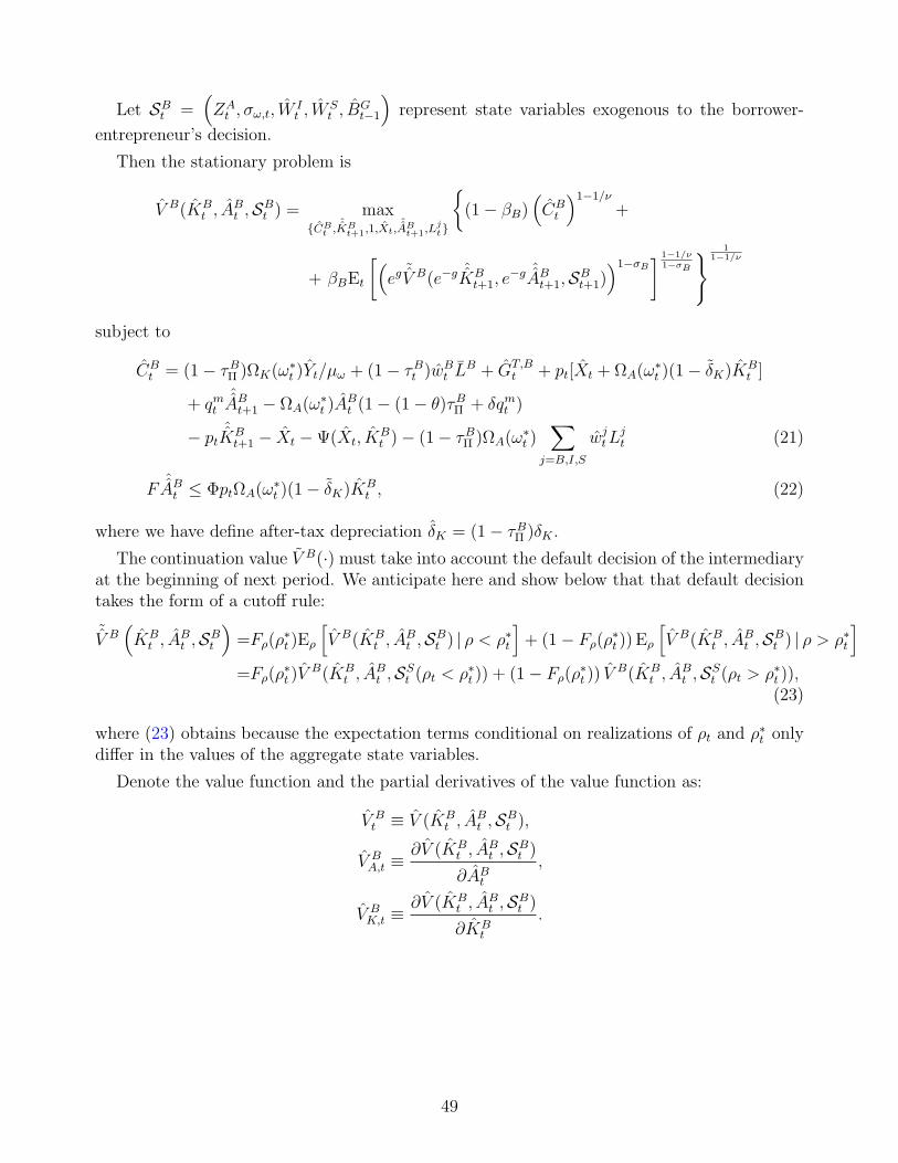
Let SBt =

(ZA

t , σω,t, WIt , W

St , B

Gt−1

)represent state variables exogenous to the borrower-

entrepreneur’s decision.

Then the stationary problem is

V B(KBt , A

Bt ,SB

t ) = maxCB

t ,ˆKB

t+1,1,Xt,ˆAB

t+1,Ljt

(1− βB)

(CB

t

)1−1/ν

+

+ βBEt

[(eg

˜V B(e−g ˆKB

t+1, e−g ˆAB

t+1,SBt+1)

)1−σB] 1−1/ν

1−σB

11−1/ν

subject to

CBt = (1− τBΠ )ΩK(ω

∗t )Yt/µω + (1− τBt )wB

t LB + GT,B

t + pt[Xt + ΩA(ω∗t )(1− δK)K

Bt ]

+ qmtˆAB

t+1 − ΩA(ω∗t )A

Bt (1− (1− θ)τBΠ + δqmt )

− ptˆKB

t+1 − Xt −Ψ(Xt, KBt )− (1− τBΠ )ΩA(ω

∗t )

∑j=B,I,S

wjtL

jt (21)

FˆAB

t ≤ ΦptΩA(ω∗t )(1− δK)K

Bt , (22)

where we have define after-tax depreciation δK = (1− τBΠ )δK .

The continuation value V B(·) must take into account the default decision of the intermediaryat the beginning of next period. We anticipate here and show below that that default decisiontakes the form of a cutoff rule:

˜V B(KB

t , ABt ,SB

t

)=Fρ(ρ

∗t )Eρ

[V B(KB

t , ABt ,SB

t ) | ρ < ρ∗t

]+ (1− Fρ(ρ

∗t )) Eρ

[V B(KB

t , ABt ,SB

t ) | ρ > ρ∗t

]=Fρ(ρ

∗t )V

B(KBt , A

Bt ,SS

t (ρt < ρ∗t )) + (1− Fρ(ρ∗t )) V

B(KBt , A

Bt ,SS

t (ρt > ρ∗t )),(23)

where (23) obtains because the expectation terms conditional on realizations of ρt and ρ∗t only

differ in the values of the aggregate state variables.

Denote the value function and the partial derivatives of the value function as:

V Bt ≡ V (KB

t , ABt ,SB

t ),

V BA,t ≡

∂V (KBt , A

Bt ,SB

t )

∂ABt

,

V BK,t ≡

∂V (KBt , A

Bt ,SB

t )

∂KBt

.

49

Therefore the marginal values of borrowing and of capital of V B(·) are:

˜V BA,t = Fρ(ρ

∗t )∂V B(KB

t , ABt ,SB

t (ρt < ρ∗t ))

∂ABt

+ (1− Fρ(ρ∗t ))

∂V B(KBt , A

Bt ,SB

t (ρt > ρ∗t ))

∂ABt

˜V BK,t = Fρ(ρ

∗t )∂V B(KB

t , ABt ,SB

t (ρt < ρ∗t ))

∂KBt

+ (1− Fρ(ρ∗t ))

∂V B(KBt , A

Bt ,SB

t (ρt > ρ∗t ))

∂KBt

Denote the certainty equivalent of future utility as:

CEBt = Et

[(eg

˜V B(KB

t+1, ABt+1,SB

t+1))1−σB

] 11−σB

.

Marginal Cost of Default Before deriving optimality conditions, it is useful to computethe marginal consumption loss due to an increased default threshold ω∗

t

∂CBt

∂ω∗t

=∂ΩK(ω

∗t )

∂ω∗t

(1− τBΠ )Yt/µω

+∂ΩA(ω

∗t )

∂ω∗t

[(1− δK)ptK

Bt − AB

t (1− (1− θ)τBΠ + δqmt )− (1− τBΠ )∑j

wjtL

jt

]

=− fω(ω∗t )

[(1− τBΠ )ω∗

t Yt/µω + (1− δK)ptKBt − AB

t (1− (1− θ)τBΠ + δqmt )− (1− τBΠ )∑j

wjtL

jt

]

=− fω(ω∗t )Ytµω

[(1− δK)ptK

Bt − AB

t (θτBΠ + δqmt )

Yt/µω

]︸ ︷︷ ︸

=Ft

=− fω(ω∗t )Ytµω

Ft.

The function Ft has an intuitive interpretation as the marginal loss, expressed in consumptionunits per unit of aggregate output, to producers from an increase in the default threshold. Thefirst term is the loss of capital due to defaulting members. The second term represents gainsdue to debt erased in foreclosure.

A.1.4 First-order conditions

Loans The FOC for loansˆAB

t+1 is:

qmt(uBt )

1−1/ν

CBt

(1− βB)(VBt )1/ν =

λBt F − βBEt[(eg ˜V B

t+1)−σB ˜

V BA,t+1](CE

Bt )

σB−1/ν(V Bt )1/ν (24)

50

where λBt is the Lagrange multiplier on the constraint in (22).

Capital Similarly, the FOC for new capitalˆKB

t+1 is:

pt(1− βB)(V

Bt )1/ν(uBt )

1−1/ν

CBt

=

βBEt[(eg ˜V B

t+1)−σB ˜

V BK,t+1](CE

Bt )

σB−1/ν(V Bt )1/ν (25)

Investment The FOC for investment Xt is:

[1 + ΨX(XBt , K

Bt )− pt]

(1− βB)(UBt )1−1/ν(V B

t )1/ν

CBt

= 0,

which simplifies to

1 + ΨX(XBt , K

Bt ) = pt.

Labor Inputs Defining γB = 1− γI − γS, aggregate labor input is

Lt =∏

j=B,I,S

(Ljt)

γj .

We further compute

∂ω∗t

∂Ljt

= µω

(wj

t

Yt− ω∗

t

MPLjt

Yt

),

defining the marginal product of labor of type j as

MPLjt = αγjµωZ

At

Lt

Ljt

(KB

t

Lt

)1−α

.

The FOC for labor input Ljt is then

(1− βB)(uBt )

1−1/ν(V Bt )1/ν

CBt

[(1− τBΠ )ΩK(ω

∗t )MPLj

t/µω − (1− τBΠ )ΩA(ω∗t )w

jt +

∂ω∗t

∂Ljt

∂CBt

∂ω∗t

]= 0,

which yields

(1− τBΠ )ΩK(ω∗t )MPLj

t/µω = (1− τBΠ )ΩA(ω∗t )w

jt + fω(ω

∗t )(wj

t − ω∗tMPLj

t

)Ft. (26)

51

A.1.5 Marginal Values of State Variables and SDF

Loans Taking the derivative of the value function with respect to ABt gives:

V BA,t =

[−(1− (1− θ)τ IΠ + δqmt

)ΩA(ω

∗t ) +

∂ω∗t

∂ABt

∂CBt

∂ω∗t

](1− βB)(u

Bt )

1−1/ν(V Bt )1/ν

CBt

= −[(1− (1− θ)τ IΠ + δqmt

)ΩA(ω

∗t ) + fω(ω

∗t )Ft

] (1− βB)(uBt )

1−1/ν(V Bt )1/ν

CBt

, (27)

where we used the fact that∂ω∗

t

∂ABt

= 1

Yt/µω.

Capital Taking the derivative of the value function with respect to KBt gives:

V BK,t =

[ptΩA(ω

∗t )(1− (1− τBΠ )δK

)+ (1− τBΠ )(1− α)ΩK(ω

∗t )Z

At

(KB

t

Lt

)−α

−ΨK(XBt , K

Bt ) +

∂CBt

∂ω∗t

∂ω∗t

∂KBt

+ λBt Φpt(1− δK)

(ΩA(ω

∗t ) + KB

t

∂ΩA(ω∗t )

∂ω∗t

∂ω∗t

∂KBt

)](1− βB)(u

Bt )

1−1/ν(V Bt )1/ν

CBt

.

Taking the derivative

∂ω∗t

∂KBt

= −µωω∗t

Yt(1− α)ZA

t

(KB

t

Lt

)−α

,

we get

V BK,t =

ptΩA(ω

∗t )(1− δK)

(1 + ΦλBt

)+ (1− τBΠ )(1− α)ΩK(ω

∗t )Z

At

(KB

t

Lt

)−α

−ΨK(XBt , K

Bt )

+(1− α)fω(ω∗t )ω

∗t

[ZA

t

(KB

t

Lt

)−α

Ft + λBt Φpt(1− δK)

](1− βB)(u

Bt )

1−1/ν(V Bt )1/ν

CBt

.

(28)

SDF We can define the stochastic discount factor (SDF) from t to t+ 1 of borrowers, condi-tional on a particular realization of ρt+1 as:

MBt,t+1(ρt+1) = βBe

−σBg

(uBt+1(ρt+1)

uBt

)1−1/ν(CB

t+1(ρt+1)

CBt

)−1(V Bt+1(ρt+1)

CEBt

)1/ν ( ˜V Bt+1

CEBt

)−σB

(29)

Conditional on information at time t, every endogenous random variable at t+1 is adaptedboth to TFP level ZA

t+1 and to the event 1[ρt+1 < ρ∗t+1]. For any such variable we define thesum

xt+1 = 1[ρt+1 < ρ∗t+1](xt+1 | ρt+1 < ρ∗t+1

)+ 1[ρt+1 ≥ ρ∗t+1]

(xt+1 | ρt+1 ≥ ρ∗t+1

).

52

Hence for any payoff xt+1 we can write the appropriately discounted payoff as

MBt,t+1xt+1.

A.1.6 Euler Equations

Loans Recall that V BA,t+1 is a linear combination of V B

A,t+1 conditional on ρt being below and

above the threshold, and with each V BA,t+1 given by equation (27). Substituting in for V B

A,t+1 in(24) and using the SDF expression, we get the recursion:

qmt = λBt F + Et

MB

t,t+1

[ΩA(ω

∗t+1)

(1− (1− θ)τΠ + δqmt+1

)+ fω(ω

∗t+1)Ft+1

]. (30)

Capital Likewise, recall that V BK,t+1 is a linear combination of V B

K,t+1 conditional on ρt beingbelow and above the threshold, and with each V B

K,t+1 given by equation (28). Substituting in

for V BK,t+1 and using the SDF expression, we get the recursion:

pt = Et

MBt,t+1

pt+1ΩA(ω∗t+1)(1− δK)

(1 + ΦλBt+1

)+ (1− τΠ)(1− α)ΩK(ω

∗t+1)Z

At+1

KB

t+1

Lt+1

−α

−ΨK(XB

t+1,KB

t+1) + (1− α)fω(ω∗t+1)ω

∗t+1

ZAt+1

KB

t+1

Lt+1

−α

Ft+1 + (1− δK)ΦλBt+1pt+1

.

(31)

A.2 Intermediaries

A.2.1 Statement of stationary problem

As for borrower-entrepreneurs, we define the following transformed variables for intermediaries:

W It , C

It , A

It+1, G

T,It , BI

t .

Denote by W It intermediary wealth at the beginning of the period, before their bankruptcy

decision. Then wealth after realization of the penalty ρt is:

˜W I

t = (1−D(ρt))WIt ,

and the effective utility penalty is:ρt = D(ρt)ρt.

Let SIt =

(ZA

t , σω,t, KBt , A

Bt , B

Gt−1, W

St

)denote all other aggregate state variables exogenous to

intermediaries.

After the default decision, intermediaries face the following optimization problem over con-

53

sumption and portfolio composition, formulated to ensure stationarity:

V I(˜W I

t , ρt,SIt ) = max

CIt ,A

It+1,B

It

(1− βI)

[CI

t

eρt

]1−1/ν

+ βIEt

[(eg

˜V I(W I

t+1,SIt+1

))1−σR] 1−1/ν

1−σR

1

1−1/ν

(32)

subject to:

(1− τ I)wIt L

I +˜W I

t + GT,It = CI

t + qmt AIt+1 + (qft + τ IΠr

ft − κIBI

t <0)BIt , (33)

W It+1 = e−g

[(Mt+1 + ΩA(ω

∗t+1)δq

mt+1

)AI

t+1 + BIt

], (34)

BIt ≥ − ξqmt A

It+1, (35)

ARt+1 ≥ 0, (36)

SIt+1 = h(SI

t ). (37)

For the evolution of intermediary wealth in (34), we have defined the total after-tax payoffper bond

Mt+1 = (1− (1− θ)τ IΠ)ΩA(ω∗t+1) + Mt+1/A

Bt+1,

where Mt+1 is the total recovery value of bankrupt borrower firms seized by intermediaries, asdefined in (12).

The continuation value˜V I(W I

t+1,SIt+1

)is the outcome of the optimization problem inter-

mediaries face at the beginning of the following period, i.e., before the decision over the optimalbankruptcy rule. This continuation value function is given by:

˜V I(W I

t ,SIt ) = max

D(ρ)Eρ

[D(ρ)V I(0, ρ,SI

t ) + (1−D(ρ))V I(W It , 0,SI

t )]

(38)

Define the certainty equivalent of future utility as:

CEIt = Et

[(eg

˜V I(W I

t+1,SIt+1

))1−σI] 1

1−σI

. (39)

A.2.2 First-order conditions

Optimal Default Decision The optimization consists of choosing a function D(ρ) : R →0, 1 that specifies for each possible realization of the penalty ρ whether or not to default.

Since the value function V I(W, ρ,SRt ) defined in (32) is increasing in wealthW and decreasing

in the penalty ρ, there will generally exist an optimal threshold penalty ρ∗ such that for a givenW I

t , intermediaries optimally default for all realizations ρ < ρ∗. Hence we can equivalently

54

write the optimization problem in (38) as

˜V I(W I

t ,SRt ) =max

ρ∗Eρ

[1[ρ < ρ∗] V I(0, ρ,SI

t ) + (1− 1[ρ < ρ∗]) V I(W It , 0,SI

t )]

=maxρ∗

Fρ(ρ∗) Eρ

[V I(0, ρ,SI

t ) | ρ < ρ∗]+ (1− Fρ(ρ

∗)) V I(W It , 0,SI

t ).

The solution ρ∗t is characterized by the first-order condition:

V I(0, ρ∗t ,SIt ) = V I(W I

t , 0,SIt ).

By defining the partial inverse F : (0,∞) → (−∞,∞) of V I(·) in its second argument as(x, y) : y = F(x) ⇔ x = V I(0, y)

,

we get thatρ∗t = F(V I(W I

t , 0,SIt )), (40)

and by substituting the solution into (38), we obtain

˜V I(W I

t ,SIt ) = Fρ(ρ

∗t )Eρ

[V I(0, ρ,SI

t ) | ρ < ρ∗t

]+ (1− Fρ(ρ

∗t )) V

I(W It , 0,SI

t ). (41)

Equations (32), (40), and (41) completely characterize the optimization problem of intermedi-aries.

To compute the optimal bankruptcy threshold ρ∗t , note that the inverse value function definedin equation (40) is given by:

F(x) =

log((1− βI)C

It )− 1

1−1/νlog(x1−1/ν − βI(CE

It )

1−1/ν)

for ν > 1

(1− βI)log(CIt ) + βI log(CE

It )− log(x)− (1− βI) if ν = 1.

Optimal Portfolio Choice The first-order condition for the short-term bond position is:

(qft + τΠrft − κIBI

t <0)(1− βI)(V

It )

1/ν

(CIt )

1/ν=

λIt + βIEt[(eg ˜V I

t+1)−σI ˜V I

W,t+1](CEIt )

σI−1/ν(V It )

1/ν (42)

where λIt is the Lagrange multiplier on the borrowing constraint (35).

The first order condition for loans is:

(qmt + τΠrmt F )

(1− βI)(VIt )

1/ν

(CIt )

1/ν= λIt ξq

mt + µI

t

+ βIEt[(eg ˜V I

t+1)−σI ˜V I

W,t+1

(Mt+1 + δΩA(ω

∗t+1)q

mt+1

)](CEI

t )σI−1/ν(V I

t )1/ν , (43)

where µIt is the Lagrange multiplier on the no-shorting constraint for guaranteed loans (36).

55

A.2.3 Marginal value of wealth and SDF

Differentiating (41) gives the marginal value of wealth

˜V IW,t = (1− Fρ(ρ

∗t ))

∂V I(W It , 0,SI

t )

∂W It

,

where∂V I(W I

t , 0,SIt )

∂W It

= (CIt )

−1/ν(1− βI)(VI(W I

t , 0,SIt ))

1/ν ,

The stochastic discount factor of intermediaries conditional on ρt+1 ≥ ρ∗t+1 is therefore

MIt,t+1 = βIe

−σIg

(V I(W I

t+1, 0,SIt+1)

CEIt

)1/ν ( ˜V I(

˜W I

t+1,SIt+1)

CEIt

)−σI (CI

t+1

CIt

)−1/ν

.

A.2.4 Euler Equations

It is then possible to show that the FOC with respect to BIt and AI

t+1, respectively, are:

qft = λIt + Et

[(1− Fρ(ρ

∗t+1))MI

t,t+1

]+ κIBI

t <0 − τΠrft , (44)

qmt (1− ξλIt ) = µIt + Et

[(1− Fρ(ρ

∗t+1))MI

t,t+1

(Mt+1 + δΩA(ω

∗t+1)q

mt+1

)]. (45)

A.3 Savers

A.3.1 Statement of stationary problem

For savers, we define the following transformed variables:

W St , C

St , B

St , G

T,St .

Let SSt =

(ZA

t , σω,t, KBt , A

Bt , W

It , B

Gt−1

)be the saver’s state vector capturing all exogenous

state variables. Scaling by (labor-augmenting) productivity, the stationary problem of the saver– after the intermediary has made default her decision and the utility cost of default is realized– is:

V S(W St ,SS

t ) = maxCS

t ,BSt

(1− βS)

[CS

t

]1−1/ν

+ βSEt

[(eg

˜V S(W S

t+1,SSt+1)

)1−σS] 1−1/ν

1−σS

11−1/ν

56

subject to

CSt = (1− τSt )w

St L

S + GT,St + W S

t − qft BSt (46)

W St+1 = e−gBS

t (47)

BSt ≥ 0 (48)

SSt+1 =h(SS

t ) (49)

As before, we will drop the arguments of the value function and denote the marginal valueof wealth as:

V St ≡ V S

t (W St ,SS

t ),

V SW,t ≡

∂V St (W S

t ,SSt )

∂W St

,

Denote the certainty equivalent of future utility as:

CESt = Et

[(eg

˜V S(W S

t ,SSt ))1−σS

].

Like borrower-entrepreneurs, savers must take into account the intermediary’s default de-cisions and the realization of the utility penalty of default. Therefore the marginal value ofwealth is:

˜V SW,t = Fρ(ρ

∗t )∂V S(W S

t ,SSt (ρt < ρ∗t ))

∂W St

+ (1− Fρ(ρ∗t ))

∂V S(W St ,SS

t (ρt > ρ∗t )

∂W St

.

A.3.2 First-order conditions

The first-order condition for the short-term bond position is:

qft (CSt )

−1/ν(1− βS)(VSt )1/ν = λSt + βSEt[(e

g ˜V St+1)

−σS ˜V SW,t+1](CE

St )

σS−1/ν(V St )1/ν (50)

where λSt is the Lagrange multiplier on the no-borrowing constraint (48).

A.3.3 Marginal Values of State Variables and SDF

Marginal value of wealth is:

V SW,t = (CS

t )−1/ν(1− βS)(V

St )1/ν , (51)

and for the continuation value function:

˜V SW,t = Fρ(ρ

∗t )∂V S(W S

t ,SSt (ρt < ρ∗t ))

∂W St

+ (1− Fρ(ρ∗t ))

∂V S(W St ,SS

t (ρt > ρ∗t )

∂W St

.

57

Defining the SDF in the same fashion as we did for borrowers, we get:

MSt,t+1(ρt+1) = βSe

−σSg

(V St+1(ρt+1)

CESt

)1/ν ( ˜V St+1

CESt

)−σS (CS

t+1(ρt+1)

CSt

)−1/ν

,

and

MSt,t+1 = 1[ρt+1 < ρ∗t+1]

(MS

t,t+1 | ρt+1 < ρ∗t+1

)+ 1[ρt+1 ≥ ρ∗t+1]

(MS

t,t+1 | ρt+1 ≥ ρ∗t+1

).

A.3.4 Euler Equations

Combining the first-order condition for short-term bonds (50) with the marginal value of wealth,and the SDF, we get the Euler equation for the short-term bond:

qft = λSt + Et

[MS

t,t+1

](52)

where λSt is the original multiplier λSt divided by the marginal value of wealth.

B Calibration Appendix

B.1 Long-term corporate Bonds

Our model’s corporate bonds are geometrically declining perpetuities, and as such have noprincipal. The issuer of one unit of the bond at time t promises to pay the holder 1 at timet+1, δ at time t+2, δ2 at time t+3, and so on. Issuers must hold enough capital to collateralizethe face value of the bond, given by F = θ

1−δ, a constant parameter that does not depend on any

state variable of the economy. Real life bonds have a finite maturity and a principal payment.They also have a vintage (year of issuance), whereas our bonds combine all vintages in onevariable. This appendix explains how to map the geometric bonds in our model into real-worldbonds by choosing values for δ and θ.

Our model’s corporate loan/bond refers to the entire pool of all outstanding corporateloans/bonds. To proxy for this pool, we use investment-grade and high-yield indices con-structed by Bank of America Merill Lynch (BofAML) and Barclays Capital (BarCap). For theBofAML indices31 we obtain a time series of monthly market values, durations (the sensitivityof prices to interest rates), weighted-average maturity (WAM), and weighted average coupons(WAC) for January 1997 until December 2015. For the BarCap indices32 we obtain a timeseries of option-adjusted spreads over the Treasury yield curve.

First, we use market values of the BofAML investment grade and high-yield portfolios tocreate an aggregate bond index and find its mean WAC c of 5.5% and WAM T of 10 years overour time period. We also add the time series of OAS to the constant maturity treasury rate

31Datastream Codes LHYIELD and LHCCORP for investment grade and high-yield corporate bonds, respec-tively

32They are named C0A0 and H0A0 for investment grade and high-yield corporate bonds, respectively.

58

corresponding to that period’s WAM to get a time series of bond yields rt. Next, we constructa plain vanilla corporate bond with a semiannual coupon and maturity equal to the WAC andWAM of the aggregate bond index, and compute the price for $1 par of this bond for eachyield:

P c(rt) =2T∑i=1

c/2

(1 + rt)i/2+

1

(1 + rt)T

We can write the steady-state price of a geometric bond with parameter δ as

PG(rt) =1

1 + rt

[1 + δPG(rt)

]Solving for PG(yt), we get

PG(rt) =1

1 + rt − δ

The calibration determines how many units X of the geometric bond with parameter δ oneneeds to sell to hedge one unit of plain vanilla bond P c against parallel shifts in interest rates,across the range of historical yields:

minδ,X

2015.12∑t=1997.1

[P c(rt)−XPG(rt; δ)

]2We estimate δ = 0.937 and X = 12.9, yielding an average pricing error of only 0.41%. This

value for δ implies a time series of durations Dt = − 1PGt

dPGt

drtwith a mean of 6.84.

To establish a notion of principal for the geometric bond, we compare it to a duration-matched zero-coupon bond i.e. borrowing some amount today (the principal) and repaying itDt years from now. The principal of this loan is just the price of the corresponding Dt maturityzero-coupon bond 1

(1+rt)Dt

We set the “principal” F of one unit of the geometric bond to be some fraction θ of theundiscounted sum of all its cash flows θ

1−δ, where

θ =1

N

2015.12∑t=1997.1

1

(1 + rt)Dt

We get θ = 0.582 and F = 9.18.

C Computational Solution

The computational solution of the model is implemented using what Judd (1998) calls “timeiteration” on the system of equations that characterizes the equilibrium of the economy. Wereduce the number of equations to the smallest feasible nonlinear system, i.e. we use linear

59

relationships between equilibrium variables to eliminate these equations, such as budget con-straints, or the relationship between the investment ratio and Tobin’s q. The remaining systemconsists of the two Euler equations for borrowers ((30) ,(31)), the three first-order conditionsfor labor demand ((26), for j = B, I, S), the two Euler equations for intermediaries ((44),(45)), the Euler equation for savers (52), no-shorting constraints for intermediaries and savers((36),(48)), the market clearing condition for risk-free debt (17), and the leverage constraintsfor intermediaries (35) and borrowers (22), respectively.

Policy functions, prices, and Lagrange multipliers are approximated as piecewise linear func-tions of the exogenous and endogenous state variables. The algorithm solves for a set of non-linear equations including the Euler equations and the Kuhn-Tucker conditions expressed asequalities. The general solution approach for heterogeneous agent models with incompletemarkets and portfolio constraints that we employ in this paper is well described by Kubler andSchmedders (2003). They show that there exist stationary equilibria in this class of modelswhen all exogenous state variables follow Markov chains, as is the case in our model as well.

The procedure consists of the following steps

1. Define approximating basis for the unknown functions. The state space consistsof

– two exogenous state variables [ZAt , σωt ], and

– five endogenous state variables [KBt , A

Bt ,W

Rt ,W

St , B

Gt ].

Denote the sets of values these state variables can take as Sx and Sn respectively. Theaggregate state space is S = Sx × Sn. There are two sets of unknown functions ofthe state variables that need to be computed. The first set of unknown functions CP :S → P ⊆ RN determines the values of endogenous objects specified in the equilibriumdefinition at every point in the state space. These are the prices, agents’ choice variables,and the Lagrange multipliers on the portfolio constraints. There is an equal number ofthese unknown functions and nonlinear functional equations. The second set of functionsCT : S × Sx → Sn determines the next-period endogenous state as a function of theendogenous state in the current period and the next-period realization of shocks. Toapproximate the unknown functions, we discretize the state space and use multivariatelinear interpolation (splines or polynomials of various orders achieved inferior resultsdue to their lack of global shape preservation). One endogenous state variable can beeliminated for computational purposes since its value is implied by the agents’ budgetconstraints, conditional on any three other state variables. As pointed out by severalprevious studies such as Kubler and Schmedders (2003), portfolio constraints lead toadditional computational challenges since portfolio policies may not be smooth functionsof state variables due to occasionally binding constraints. Hence we cluster grid points inareas of the state space where constraints transition from slack to binding, and we testthe accuracy of the approximation by computing relative Euler equation errors.

2. Iteratively solve for the unknown functions. Given an initial guess C0 = C0P , C0

T ateach point in the discretized state space compute tomorrow’s optimal policies as functionsof tomorrow’s states. Then, compute expectation terms in the equilibrium conditions

60

using quadrature methods. Next, solve the system of nonlinear equations for the current-period optimal policies. This defines the value of the next iterate C1

P at the given point.Using it, compute the next iterate of the transition approximation C1

T at the given point.Once C1 has been computed at every point on the grid, repeat until convergence in thesup norm.

The system of nonlinear equations at each point in the state space is solved using astandard nonlinear equation solver. Judd, Kubler, and Schmedders (2002) show howKuhn-Tucker conditions can be rewritten as equality constraints for this purpose. Forexample, consider the saver’s Euler Equation for risk-free bonds and constraint:

qft = λSt + Et

[MS

t,t+1

]0 ≤ BS

t

Now define an auxiliary variable xt and two functions of this variable, such that λS,+t =max0, xt3 and λS,−t = max0,−xt3. Then the two equations above can be written asequalities:

qft = λS,+t + Et

[MS

t,t+1

]0 = BS

t − λS,−t

The solution variable for the nonlinear equation solver corresponding to the constraint isxt.

The nonlinear equation solver needs to compute the Jacobian of the system at each step.Numerical central-difference (forward-difference) approximation of the Jacobian can beinaccurate and is computationally costly because it requires 2N + 1 (N + 1) evaluationsof the system, whereas analytically computed Jacobians are exact and require only oneevaluation. We follow Elenev (2017) in pre-computing expectations, which simplifies thenonlinear system such that its Jacobian can be computed analytically. This greatly speedsup calculations.

3. Simulate the model for many periods using approximated policy functions. Toobtain the quantitative results, we simulate the model for 10,000 periods after a “burn-in”phase of 500 periods. We verify that the simulated time path stays within the bounds ofthe state space for which the policy functions were computed.

In a long simulation, errors in the nonlinear equations are low. Table 8 reports the medianerror, the 95th percentile of the error distribution, the 99th, and 100th percentiles.

61

Table 8: Computational Errors

Percentile

50th 75th 95th 99th Max

(30) 0.0015 0.0043 0.0165 0.0307 0.0730

(31) 0.0004 0.0007 0.0013 0.0020 0.0056

(26) 0.0001 0.0002 0.0004 0.0005 0.0006

(26) 0.0001 0.0002 0.0004 0.0005 0.0006

(26) 0.0001 0.0002 0.0004 0.0005 0.0006

(44) 0.0251 0.0392 0.0830 0.1516 0.2119

(45) 0.0272 0.0422 0.0878 0.1597 0.2215

(52) 0.0007 0.0011 0.0020 0.0029 0.0082

(35) 0.0009 0.0028 0.0074 0.0117 0.0201

(48) 0.0033 0.0052 0.0066 0.0098 0.0129

(17) 0.0004 0.0006 0.0009 0.0010 0.0013

(36) 0.0001 0.0001 0.0004 0.0006 0.0008

(22) 0.0052 0.0170 0.0343 0.0453 0.0618

The table reports median, 75th percentile, 95th percentile,99th percentile, and maximum absolute value errors, eval-uated at state space points from a 10,000 period simula-tion of the benchmark model. The 12 equations definepolicy functions. They are a subset of the 21 equationsthat define the equilibrium.

62