Embed Size (px)
Citation preview

IMA Journal of Mathematical Control & Information (1992) 9, 275-303
A. M. Lyapunov's stability theory—100 years on*
P. C. PARKS
Royal Military College of Science (Cranfield),Shrivenham, Swindon, Wilts SN6 8LA, UK
On 12 October 1892 (by the modern calendar) Alexandr Mikhailovich Lyapunovdefended his doctoral thesis The general problem of the stability of motion at MoscowUniversity. A brief history of Lyapunov's life and tragic death is given, and followedby a section highlighting the important ideas in his thesis of 1892. Subsequentapplications of these ideas in the control field are then reviewed, from which thegreat importance of Lyapunov's thesis in present day technology may be appreciated.
AlexandrMikhailovichLyapunov,1857-1918
(Courtesy,U.S.S.R.Academy ofSciences)
| ^ |
FIG. 1.
1. A brief history of the life of A. M. Lyapunov
Aleksandr Mikhailovich Lyapunov was born on 6 June 1857f at Yaroslavl' wherehis father was director of the Demidovsk Lycee, a general high school. In 1870 hismother, who had been widowed in 1868, moved with her three sons to Nizhny-Novgorod (known for many years as Gorki), and it was here that Lyapunovreceived his secondary school education, graduating from the gymnasium in 1876with a gold medal. In the same year he became a student in mathematics at St.Petersburg University, where he was particularly influenced by the lectures of
• IMA Lyapunov Centenary Lecture given at the IMA International Conference on Control, Modelling,and Computation, UMIST, Manchester, 2-4 September 1991
t All dates in this paper accord to the modern (Gregorian) calendar.
275O Oxford Univtmty Pren 1993
at Penn S
tate University (P
aterno Lib) on August 1, 2010
http://imam
ci.oxfordjournals.orgD
ownloaded from

276 P. C. PARKS
Professor P. L. Chebyshev. Lyapunov graduated in 1880, again winning a gold medalfor an essay on hydrostatics. He stayed on at the university in the Mechanics Faculty,developing his Master's thesis On the stability of ellipsoidal forms of equilibrium ofrotating fluids which he defended in 1884 (Lyapunov 1884). This work, which wastranslated into French in 1904, established his name in Europe.
In the autumn of 1885, Lyapunov moved to Kharkov where he became a'privat-dozent' in the university's Department of Mechanics. In the winter break of1885/6 he returned to St. Petersburg to marry his first cousin, Natalia RafailovnaSechenova. In his work in Kharkov, Lyapunov first had to spend much timepreparing lectures in mechanics and notes for his students, but in 1888 he started topublish papers devoted to the stability of motion. This work led to his famousdoctoral thesis of 1892, The general problem of the stability of motion (Lyapunov1892). He defended this thesis in Moscow on 12 October 1892, one of his 'opponents'being N. E. Zhukovski (better known here as Joukowski—'the father of Russianaviation'); this thesis was republished in French in 1908 and 1949, Russian in 1935,and English (Lyapunov 1992). Lyapunov was promoted in the following year 1893to an ordinary professorship at Kharkov.
Although Lyapunov continued his work on stability problems until 1902, he alsoturned his attention to other topics, including potential theory and probability theory,particularly the central limit theorem of Laplace. He was also an active participantin activities of the Kharkov Mathematical Society, becoming its president and editorof its Communications from 1899 to 1902.
In 1902, Lyapunov moved back to St. Petersburg where he had been appointedAcademician and the successor to his former teacher P. L. Chebyshev, who had diedin 1894. He was now able to devote himself entirely to research, returning to theproblem of forms of equilibrium of bodies of uniformly rotating fluid particles undermutual Newtonian gravitational attraction. In particular, Lyapunov showed thatpear-shaped forms of rotating fluid were unstable. This result had importantconsequences in astronomy, since it disproved the then current theories of formationof satellites from bodies of rotating fluid e.g. the Earth-Moon system. G. H. Darwin(son of the famous naturalist Charles Darwin) at Cambridge had proposed such amechanism at this time which naturally required pear-shaped bodies to be stable. In1917, J. H. Jeans, in an Adams Prize Essay at Cambridge, was to confirm thatLyapunov's result was correct and that therefore Darwin's theory was incorrect.
In June 1917, Lyapunov left St. Petersburg for Odessa on doctor's orders, sincehis wife was suffering badly from tuberculosis. However, in Odessa her conditiondeteriorated, and on 31 October 1918 she died. Lyapunov himself was in poor healthand his eyesight was failing. The tragic events of the revolution, the burning of thefamily estate on the River Volga including a great library built up by his father andgrandfather, and the illness of his wife had greatly depressed Lyapunov. On the dayhis wife died, Lyapunov shot himself in the head with a pistol. He died on 3 November1918, the day of his wife's funeral. In a suicide note he asked to be buried with her.The inscription on the gravestone reads:
The creator of the theory of stability of motion, the doctrine of equilibrium figures ofrotating liquid, methods of the qualitative theory of differential equations, author of the
at Penn S
tate University (P
aterno Lib) on August 1, 2010
http://imam
ci.oxfordjournals.orgD
ownloaded from

A. M. LYAPUNOV'S STABILITY THEORY—100 YEARS ON 277
central limit theorem and other deep investigations in areas of mechanics and mathe-matical analysis.
At this time, many of the later uses of Lyapunov's work could hardly have beenforeseen. Some of these will be described in later sections of this paper.
2. Lyapunov's doctoral thesis The general problem of the stability of motion
The thesis was first published by the Kharkov Mathematical Society (Lyapunov1892). A translation into French by E. Davaux was published by the University ofToulouse in 1908; this translation was reprinted as a book by Princeton UniversityPress in 1949. In March 1992, the International Journal of Control devoted its entireissue to an English translation by A. T. Fuller of the French version (Lyapunov1992). In the same issue, J. F. Barrett provided both a translation from Russian ofa biography of Lyapunov by Academician V. I. Smirnov and a bibliography of allLyapunov's works. Lyapunov's thesis runs to 242 printed pages in this Englishversion. A number of important ideas are contained in the thesis, of which thefollowing four topics may be highlighted.
2.1 General definitions of stability of motion
Lyapunov's thesis opens with some rather general definitions of the stability ofmotion. These include various measures of stability of a point following a particulartime trajectory in an n-dimensional space. It is possible for a certain motion to bestable with respect to some measures but unstable with respect to others. HereLyapunov gives as an example a particle in a circular orbit under an inverse-squarelaw of attraction: this motion is stable with respect to the length of the radius vectorand to the speed of the particle, but is unstable with respect to the rectangularcoordinates of its position.
Stability, in the sense of points in phase-space which are initially close togethersubsequently staying close together, is lacking even in apparently well-behavedHamiltonian systems where
m dHxt = — and pi = —— (i = 1 ,..., n). (1)
dp, dxiConsequently phase-space volumes v are preserved, because
v(t) = D(0) exp trace Jdx = v(0)t
Josince
, - / d2H d2H \ ntrace / = Y = 0,i=i\dx, dp, dp,dxtj
where J is the Jacobian matrix formed from the right-hand sides of the Hamiltonianequations. This result was originally due to Liouville (1809-82). Figure 2, from
at Penn S
tate University (P
aterno Lib) on August 1, 2010
http://imam
ci.oxfordjournals.orgD
ownloaded from

278 P. C. PARKS
FIG. 2 Diffusion of trajectories.
Penrose (1990), shows how this volume preservation can nevertheless allow extensivediffusion of the trajectories in phase space (of dimension 2n).
2.2 Characteristic numbers of functions and 'Lyapunov exponents'
This second concept, also developed quite early on in Lyapunov's thesis, is called byhim the 'characteristic number' of a function of time. Given a function x(t), then onecan define Xo such that x(t) exp Xt is unbounded for X > Xo and x(t) exp Xt -* 0 ast —> oo for X < Xo. The critical (real) number Xo is the characteristic number of x(t).For example, if x(t) = t2, then Xo — 0; if x(t) = exp( — 2r), then Xo = 2; and ifx(t) = exp(t sin t), then Xo = — 1.
In recent years, the term 'characteristic exponent' or 'Lyapunov exponent' hasbeen used in the context of chaotic motion. Here one is interested in whether or nottwo points Xi(t) and x2(t) in the state space of a dynamical system which are initiallyvery close together, stay close together in the subsequent motion. Here the functionof time, x(t), being considered is given by x(t) = |x,(0 — x2(t)\, where Ix^O) — x2(0)|is 'small'. The largest characteristic or Lyapunov exponent can be defined as
l i m l n
,^t M O ) - x2(0)|A chaotic motion is characterized by a positive Lyapunov exponent, which can be
regarded as minus one times the characteristic number as originally denned byLyapunov himself, and explained in the previous paragraph. Thus, in a chaoticmotion, the two points move apart as time increases, making accurate prediction ofthe long term future impossible. More generally, for various attractors in state spacemotions in an n-dimensional space R", a set of n Lyapunov exponents may be defined,
at Penn S
tate University (P
aterno Lib) on August 1, 2010
http://imam
ci.oxfordjournals.orgD
ownloaded from

A. M. LYAPUNOV'S STABILITY THEORY—100 YEARS ON 279
Fixed point
\ /
/ \
Torus
(0.0,-)
Limit cycle
o.__}—
(0.-.-)
Strange attractor
(+.0.-)
FIG. 3. Signs of Lyapunov exponents for various attractors.
and their signs characterize the attractor. This idea is illustrated for three-dimensionalstate space in Fig. 3, taken from Ruelle (1989).
2.3 Lyapunov's first method
Lyapunov's first method provides theoretical validity for the often-used technique oflinearization. More precisely, given a set of nonlinear first-order differential equations
*t=fi(xl,...,xll) ( i=l , . . . ,n), (2)
where the /( are analytic functions such that /,(0,..., 0) = 0 (i = 1 ,...,«), so that theongin x = 0 is an equilibrium point, then a linearized set of equations
x = Jx
may be found by forming the Jacobian matrix J with the (i,j) entry
J - {i,j= 1 ,..., n),
or, equivalent^, by expanding the /, as a power series about x = 0 and dropping allterms except those linear in the x,s.
at Penn S
tate University (P
aterno Lib) on August 1, 2010
http://imam
ci.oxfordjournals.orgD
ownloaded from

280 P. C. PARKS
If the matrix / has all its eigenvalues either negative or with negative real parts,so that the linearized equation (3) is asymptotically stable, then so will be the originalnonlinear equation (2), at least for initial conditions x lying in a finite region aboutthe origin, that is to say, initial displacements x from the origin within this regionwill decay to zero as time tends to infinity.
Lyapunov has an involved proof of this result involving a solution in series of theoriginal nonlinear equation in which the /, may also be functions of time. He alsoexamines at some length various 'singular cases', that is, cases in which / haseigenvalues which are zero or have zero real parts. Here stability is determined bythe nonlinear terms in the power-series expansion of the /,. Specifically, the cases ofone zero eigenvalue and of two purely imaginary eigenvalues, ±]X, were consideredin the thesis.
2.4 Lyapunov s second method
'The fourth highlight of Lyapunov's thesis has proved subsequently to be the mostimportant—this is his so-called 'second' or 'direct' method, making use of'Lyapunovfunctions'. Once again, if we consider x = 0 to be an equilibrium point of thenonlinear differential equation (2), then it may prove possible to investigate thestability of this equilibrium point by examining a positive-definite function V = V(x),surrounding x = 0 with a nest of closed surfaces defined by V(x) = c (c > 0). The rateof change with respect to time of V following a trajectory of (2) is easily calculated as
If this is always negative (except at x = 0, where V = 0), then it follows that thetrajectories must cross the surface V = constant in an inwards directions, andconsequently tend to the point x = 0 at time t tends to infinity. A three-dimensionalexample is shown in Fig. 4. Thus asymptotic stability has been proved without anyneed to find explicit solutions of the nonlinear differential equation (2).
This powerful idea originated in Lyapunov's mind from his knowledge ofastronomical problems and the earlier work of Lagrange, Laplace, Dirichlet, andLiouville (Fuller 1992). In many astronomical problems, stability—rather thanasymptotic stability—is sought; in such cases, V is zero so that the disturbed motionspersist as oscillations on some surface V = c surrounding JC = 0. The greater interestin asymptotic stability shown in contemporary control theory did not developuntil the 20th century.
3. Applications of Lyapunov's second method in control theory—developments inRussia before 1960
3.1 Chetayev's work at Kazan (1930s)
Lyapunov's (1892) thesis contains many mathematical examples of his theory notlinked with physical stability problems (although Fuller's (1992) English translationadds an occasional control-engineering interpretation of Lyapunov's examples (e.g.
at Penn S
tate University (P
aterno Lib) on August 1, 2010
http://imam
ci.oxfordjournals.orgD
ownloaded from

A. M. LYAPUNOV'S STABILITY THEORY—100 YEARS ON 281
Trajectories
FIG. 4. Liapunov function contours and trajectories of x =f(x).
in Section 41, Examples V and VI)). Practical use of Lyapunov's stability theory inthe control field came many years later, notably in the work of N. G. Chetayev andI. G. Malkin at the Kazan Aviation Institute in the 1930s (Chetayev 1961; Malkin1952). A typical example of Chetayev's application of Lyapunov's second methodto aeronautical stability problems is provided by the classical problem of spinstabilization of a rocket or artillery shell. The (simplified) model is shown in Fig. 5.The corresponding equations of motion, obtained from the moving-axes equation
FIG. 5. Rotating rocket stability problem.
at Penn S
tate University (P
aterno Lib) on August 1, 2010
http://imam
ci.oxfordjournals.orgD
ownloaded from

282 P. C. PARKS
for angular momentum in conventional notation, are
Af! + Ad2 sin /? cos /? - Cnd cos /? = eR sin /? cos a,
Ad — 2Adfi sin fi + Cnfi = eR sin a,
where A, C, n, e, and R are constants. Now two integrals of the motion exist, identifiedas energy F, and angular momentum F2:
+ <*2 cos2 /?) + eR(cos a cos 0 - 1)
F2 = A(/J sin a — a cos ft sin ^ cos a) + Cn(cos a cos ^ — 1).
A tentative Lyapunov function is formed as V = F, — AF2, with V = 0. Expandingthe trigonometric terms in F! and F2 gives
+ (Cnl - eR)a2 -+ (CnX - eR)P2 + 2AMP]
+ higher-order terms.
[ A ±A/i ~]
. Each±Ak CnX — eRj
of these is positive definite if A > 0 and — AeR + ACnX - A2k2 > 0. A suitableconstant k can be found if Ak1 — Cnk + eR = 0 has two real roots, from which isobtained the (well known) criterion for spin stabilization:
C2n2>4AeR.
3.2 Contributions of Lufe and Letov
A nonlinear control problem discussed extensively by A. I. Lur'e (1957) and A. M.Letov (1961) and dating back to the 1940s is illustrated in Fig. 6.
If we consider the demand nD to be zero, then the stability of the feedback loopmay be investigated by examining the nonlinear differential equations
y = Ky + <* =/(a) , a = pTy - (4)
FIG. 6. The Lur'e-Letov nonlinear control problem.
at Penn S
tate University (P
aterno Lib) on August 1, 2010
http://imam
ci.oxfordjournals.orgD
ownloaded from

A. M. LYAPUNOV'S STABILITY THEORY—100 YEARS ON 283
where A" is a constant matrix, m and p are constant vectors, and r is a non-negativereal number. The equations are first transformed by the 'generalized Lur'e trans-formation'
y = Dx - Db£,
where D is any non-singular matrix such that Db = K~ 1m, to yield
x = Ax + bf{a), 6 = cTx- rf{a), (5)
where A = D~iKD. The nonlinearity f{&) is assumed to be continuous in a, with/(0) = 0, of(<r) > 0 (<x # 0), and J? f(a) da infinite. A Lyapunov function V isintroduced as
V=xTBx+ I f(<b)d<b,
with V= -xTCx + 2f(a)gTx +f(a)cTx - rf\a), where ATB + BA = - C and# = Bb. The matrix C is positive-definite, and B also, if we assume that KT (andA = D~lKD) has all its eigenvalues with negative real parts. The Lyapunov derivativeV may be made negative-definite, either (if c is given) by choosing the feedbackconstant r such that
r>{gT +kcT)C~\g + \c),
or (if r is given) by choosing the vector c as
where vTv < 1 and C = TTT, with T nonsingular.
3.3 Aizermaris conjecture
The problem considered by Lur'e and Letov led M. A. Aizerman (1949) to make afamous conjecture concerning the function f{a) appearing in equation (4) and Fig. 6.This conjecture, as applied to this problem, is as follows. 'If f{a) is replaced by alinear function ka, and if the resulting linearized form of (4) is asymptotically stablefor all constant k in the sector 0 < k < K, then the nonlinear system (4) will also beasymptotically stable.' Here K is a constant such that 0 < of {a) < Ka2 (a # 0); seeFig. 7.
Unfortunately the general Aizerman conjecture is untrue; the following counter-example was found by Krasovskii (1963), which is in a form different from equations(4) and (5). Consider
X2 = ~Xi — X2 .
If / ( x j is replaced by kxt then 0 < k < 1 ensures asymptotic stability. However, if
fx - [e - 2 / ( l +e~l)]x for |x| < 1,flx) =
U - [e~2W/(l + e- |x |)]signx for |x| ^ 1,then 0 < xf(x) < x2 (x / 0), but the trajectory starting at xl = 1 and x2 = e~l — 1has the equation
at Penn S
tate University (P
aterno Lib) on August 1, 2010
http://imam
ci.oxfordjournals.orgD
ownloaded from

284
FIG. 7. f(a) for Aizerman's conjecture.
and oo and x2 — oo as t
= e
oo.
- X l
Aizerman's conjecture stimulated later developments, in particular Popov'sstability criterion (see Section 4.4).
4. Lyapunov's second method in control theory—developments since 1960 (mainly
outside Russia)
4.1 Introduction
These developments started in the late 1950s and early 1960s and were greatlystimulated by challenging control problems associated with the so-called 'space race'between the USA and USSR, set off by the launch of the Soviet Sputnik 1 (4 October1957). Of particular significance in making Lyapunov's second method better knownoutside Russia were the 1st World Congress of the International Federation ofAutomatic Control (IFAC), held in Moscow in June 1960, and a seminal article byR. E. Kalman and J. E. Bertram in the Journal of the American Society of MechanicalEngineers, published in the same month (Kalman & Bertram 1960). A group formedby Professor Solomon Lefschetz at the Research Institute for Advanced Study atBaltimore USA (of which R. E. Kalman and J. P. La Salle were members) wasparticularly active at this time in making Russian mathematical techniques betterknown. Cover-to-cover English translations of selected Russian journals also startedin these years. A very readable book on Lyapunov's second method by Lefschetz andLa Salle appeared in 1961.
4.2 The Lyapunov Hermite-Routh-Hurwitz connection
A question raised by Kalman & Bertram (1960) was how Lyapunov's second methodcould be employed to recover classical results for linear differential equations suchas those derived by E. J. Routh (1877) and by A. Hurwitz (1895). The connection
at Penn S
tate University (P
aterno Lib) on August 1, 2010
http://imam
ci.oxfordjournals.orgD
ownloaded from
A. M. LYAPUNOV'S STABILITY THEORY—100 YEARS ON 285
was firmly established by P. C. Parks (1964b) using a special solution of the Lyapunovmatrix equation (see also Section 4.3).
If the nth-order linear differential equation with real constant coefficients isgiven by
p(D)y = (iy + fliD""1 + a2D"-2 +•••+ an)y = 0, (6)
and its phase-space form by x = Ax, where
r o i o ••• o n0 0 1 - 0
A= \ : - ••. - (7)
0 0 0 - 1
is the companion matrix of (6). Then a Lyapunov function is V = xTHx, where
! Q _ i U Q Q _ i U ' " ' " " '
0 — ^ B ^ B — 3 ~r" &w— l "•— i 0 **• '"
0 a3
— a3 + aiO2 0
0 a,
(8)
in which the (i, j ) element is
' n - l
)*+" 'a*a2.-(-j-* + i (' + ; even, i > ; ) ,
(i +j odd, i >;'),
where a0 = 1 and ar = 0 for r > n. Here /^ is Hermite's (1856) matrix, and
V = xT(HA +ATH)x= -2(alxn + a3xm.2+~)2.
Clearly, V is negative semidefinite and, provided that a} # 0 for some odd j , can beshown not be identically zero on any trajectory other than x = 0, from whicha necessary and sufficient condition for stability is that H is positive definite.
at Penn S
tate University (P
aterno Lib) on August 1, 2010
http://imam
ci.oxfordjournals.orgD
ownloaded from

286 P. C. PARKS
The principal minors of H starting from the bottom right-hand corner areAu AtA2, A2A3,..., An_xAn where the A, are the Hurwitz determinants of the equation(6). For stability, the A{ must all be positive and p(s), appearing as p(D) in (6), isthen said to be a 'Hurwitz polynomial'. The Hermite matrix was used by B. D. O.Anderson (1972) to prove the Lienard-Chipart stability criterion and by M. Mansourand Anderson (1992) to provide a Lyapunov proof of the celebrated Kharitonovtheorem (1978).
4.3 Construction of Lyapunov functions
The first applications of Lyapunov's second method used integrals of motion, suchas energy and momentum, or quadratic forms and integrals of the nonlinearity as inthe Lur'e and Letov technique. In the 1960s, considerable efforts were made to devisesystematic methods of construction of Lyapunov functions.
The Lyapunov matrix equation Given nonlinear equations of the form
x=f(x) (9)
with x € W and /(0) = 0, one can usually extract the linear part in the form of thematrix equation
x = Ax. (10)
If A has all its eigenvalues with negative real parts, then the origin x = 0 is anasymptotically stable equilibrium point of (10) and of (9) also. A suitable Lyapunovfunction for (9) may however yield other useful information such as an approximationto the region of attraction surrounding x = 0. Such a Lyapunov function can be aquadratic form xrPx, where P is found by solving the Lyapunov matrix equation
PA+ATP=-Q, (11)
in which Q is a given arbitrary symmetric positive-definite matrix. This involvessolving \n(n + 1) linear equations for the elements pu (j ^ 1) of the symmetric matrixP. (This is always possible, provided that A, + kj =£ 0 for any i and j , where the A,are the eigenvalues of A.)
S. Barnett and C. Storey (1967) introduced a new way of solving (11) in the form
where S is the unique skew-symmetric matrix satisfying
SA + ATS = i-(ArQ-QA). (12)
Solving equation (12) involves the solution of \n{n — 1) linear equations for theelements of 5: a reduction of n compared with the solution of (11). More importantly,Barnett & Storey (1968) were able to exploit this idea to investigate the sensitivityor robustness of the stability of (10).
An early application of the Lyapunov matrix equation was due to A. G. J.MacFarlane (1963). He constructed performance functionals for the stable linear
at Penn S
tate University (P
aterno Lib) on August 1, 2010
http://imam
ci.oxfordjournals.orgD
ownloaded from

A. M. LYAPUNOV'S STABILITY THEORY—100 YEARS ON 287
system (10) in the form
" trxTQxdt = (-iy+1xT(0)P r+1x(0),
where P,+ XA + ATPI+1 = P, (s = 1 ,..., r) and PXA + ATPX = Q.A typical application of the Lyapunov matrix equation to examine the effect of
bounded disturbances is the paper by P. A. Cook (1980). As an example, he consideredthe damped pendulum equation
x + 2«x + sin x = u(t)
with \u(t)\ < k for all (. A suitable quadratic Lyapunov function V is found using (11)with Q = 2el and then, from V, a sufficient condition on k to ensure that |x| J% V forall t is
k < veN/(l — e2) — Kv ~ s ' n v)-
Integration by parts An important development in the construction of Lyapunovfunctions was introduced by R. W. Brockett (1970). His result may be stated asfollows: given the linear constant-coefficient /ith-order differential equation
p(D)y = 0, (13)
where p(D) takes the form of equation (6) given earlier, then a Lyapunov functionfor (13) is
V(x) = j {q(D)yp(D)y - [r(D)y]2} dt,
where x is the phase-space vector [y, Dy,..., D"~ly']T, q(s)/p(s) is a positive-realfunction, and
with Ev(») denoting the even part of the polynomial (•) and r(s) being aHurwitz polynomial. The importance of this technique is its connection withfrequency response, since it is a property of the positive-real function q(s)/p(s) thatRe[g(ja>)/p(ja;)] ^ 0 for all real a>.
We note that some special choices of q(s) are possible: if q{s) is chosen as thepolynomial a,*""1 + a3s"~3 + a5s"~5 +••• formed from p(s) by deleting alternateterms, then V = \xTHx, using the special Hermite form H given earlier in equation (8).On the other hand, if (̂5) is chosen as (d/ds)p(s) = ns"~l + a^n — l)s"~2 H 1- a,,then it turns out that V = —xTHx; i.e. H turns up in V rather than V (Parks 1969),so that the sufficient conditions obtained from V are in fact necessary as well.
The variable-gradient method Of more general methods of constructing Lyapunovfunctions, the so-called variable-gradient method of D. G. Schultz and J. E. Gibson(1962) is prominent. Here the gradient of V, that is the vector
* = gradK= — , . . , — ,
at Penn S
tate University (P
aterno Lib) on August 1, 2010
http://imam
ci.oxfordjournals.orgD
ownloaded from

288 P. C. PARKS
is considered as g = [gx{x),..., gn(x)]T, with the gt(x) given as
that is, as quasi-linear forms in xt,..., xB. Two sets of conditions are imposed on g:first, it has to be the gradient of a scalar function (V) so that the n x n curl matrixof g is zero, i.e.
and secondly V = gTx ^ 0, so that V is negative-definite or negative-semidefinite. Vmay be found by integration along any path from the origin to the general point x(usually the path is chosen, for convenience of the integration, as parallel to each x,axis in turn).
A variant of this procedure is due to D. R. Ingwerson (1961): here the Jacobianmatrix
J{x) =
is calculated from (9) to give
x = J(x)x. (14)
The Lyapunov matrix equation JT(x)P(x) + P(x)J(x) = — Q is solved for P{x), anda new matrix Pi(x) is formed from P(x) by putting all xk = 0 in {P{x))u except x,and Xj. The procedure then follows that of the variable-gradient method, taking
9,(x)= t PVi(*,,^))udSj,J=i Jo
the curl matrix being identically zero from the construction of gt.
The Zubov Method In a series of papers culminating in a book, V. I. Zubov (1962)developed a scheme for solving the partial differential equation
where 9(x) is a positive-definite or positive-semidefinite function. In particular, if f(x)can be developed as a power series in the components x, of x, then V can also be sodeveloped. In general, there is the danger of a combinatorial explosion in doing this,but in simple examples the method works well and, in some cases, exact domains ofattraction can be found.
4.4 Popov's stability criterion
Important developments by V. M. Popov (in Romania) and R. E. Kalman (in theUSA) led to a connection between frequency response and the existence of Lyapunov
at Penn S
tate University (P
aterno Lib) on August 1, 2010
http://imam
ci.oxfordjournals.orgD
ownloaded from

A. M. LYAPUNOV'S STABILITY THEORY—100 YEARS ON
U-0
289
-*-<7(s)P(s)
FIG. 8. Feedback loop for Popov's criterion.
functions. A neat form of these results is due to Brockett (1964) for the feedback loopshown in Fig. 8, and may be stated as a theorem:
The null solution of the system shown in Fig. 8 is asymptotically stable for alladmissible f(a) if there is an a > 0 such that (1 + <xs)G(s) is a positive-realfunction.
The key property of a positive-real function Z(s) is that Re Z(jco) ^ 0 for all real a>.The theorem leads to the graphical interpretation of Fig. 9, showing the modifiedNyquist plot of G(ja)), in which to Im G(ja») is plotted against Re G(j(o). In Fig. 9, thismodified Nyquist plot must lie to the right of a straight line through the origin withslope I/a—the 'Popov line'—for asymptotic stability, as stated in the theorem. Infact, this condition ensures the existence of a Lyapunov function of the type 'quadraticform plus integral of the non-linearity', the quadratic form being found by Brockett's'integration by parts' technique.
If the non-linearity can be confined so that
0 < of (a) < ka2 (a # 0),
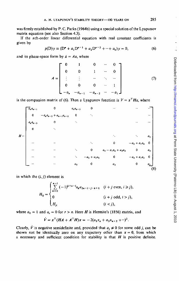
then a relaxation of the Popov condition may be made by moving the Popovline a distance l//c to the left of the origin of the modified Nyquist diagram asshown in Fig. 10. For example, if G(s) in Fig. 8 is l/(s3 + as2 + bs), with a,b > 0,
FIG. 9. Popov line.
at Penn S
tate University (P
aterno Lib) on August 1, 2010
http://imam
ci.oxfordjournals.orgD
ownloaded from
290 P. C. PARKS
FIG. 10. Displaced Popov line.
then the closed loop is asymptotically stable, provided that 0 < af{a) < aba2
for a # 0.
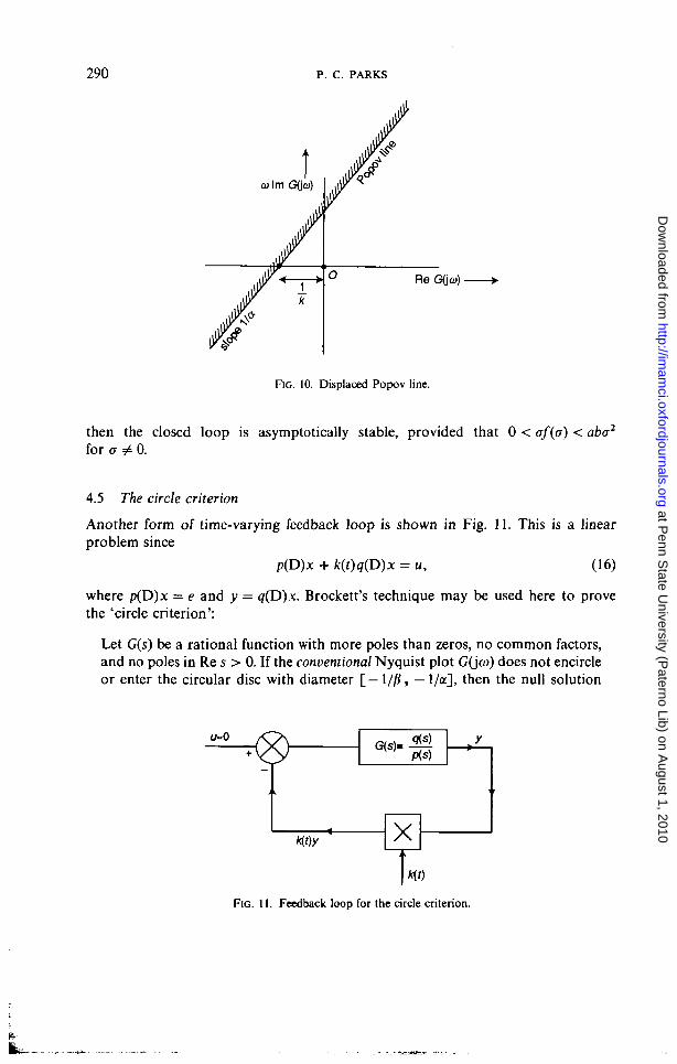
4.5 The circle criterion
Another form of time-varying feedback loop is shown in Fig. 11. This is a linearproblem since
p(D)x + k(t)q{D)x = u, (16)
where p(D)x = e and y = <j(D)x. Brockett's technique may be used here to provethe 'circle criterion':
Let G(s) be a rational function with more poles than zeros, no common factors,and no poles in Re s > 0. If the conventional Nyquist plot G(ja>) does not encircleor enter the circular disc with diameter [—1/)?, —I/a], then the null solution
X| MO
FIG. 11. Feedback loop for the circle criterion.
at Penn S
tate University (P
aterno Lib) on August 1, 2010
http://imam
ci.oxfordjournals.orgD
ownloaded from

A. M. LYAPUNOV'S STABILITY THEORY—100 YEARS ON
FIG. 12. The circle criterion.
of equation (16) (with u = 0) is uniformly asymptotically stable if
0 ^ $ + e </(t) ^ a - e < oo
for some e > 0.
This criterion is illustrated in Fig. 12, which shows the location of the circular discin the complex plane.
4.6 Sampled-data or discrete-time systems
Lyapunov functions may be constructed also for discrete-time systems. If the discretetime is taken as . . . , t — 1, t, t + 1, t + 2,..., then the 'derivative' of the Lyapunovfunction V, is taken as the difference V, — V,_x. Again quadratic forms may often beused; so, for example, the stable linear discrete-time system
has a Lyapunov function xJPx,, where P satisfies the discrete-time Lyapunov matrixequation
ATPA - P= -Q, (18)
in which Q is positive-definite or positive-semidefinite. By a suitable choice of Q, thenecessary and sufficient stability condition that P is positive-definite can be identifiedas the classical Shur-Cohn stability criterion for the eigenvalues of A to lie withinthe unit circle of the complex plane (Parks 1964a; Jury 1974).
4.7 Special Lyapunov functions
Occasionally, special types of Lyapunov function may be employed. A good exampleis the Lyapunov function
V=t\*i\ O9)
at Penn S
tate University (P
aterno Lib) on August 1, 2010
http://imam
ci.oxfordjournals.orgD
ownloaded from

292 P. C. PARKS
devised by H. H. Rosenbrock (1963). If this is applied to the linear system
x = Ax, (20)
then it is sufficient to check that the trajectories of (20) are directed inwards at allthe vertices of the hypercubes defined by V = constant surrounding x = 0. This willbe so if
<*jj + t K\ < ~EJ < 0 0 = 1 >•••> «)• (21)
An alternative Lyapunov function of a simple type is
V = max |x,|,i
when the condition corresponding to (21) is
au+ t K K - e , < 0 (i = 1 ,..., ii). (22)
Inequalities (21) and (22) will be recognized as Gershgorin's (1931) sufficientconditions for the stability of (20).
4.8 Lyapunov functions for partial differential equations
Many important physical processes are described by partial differential equations asopposed to ordinary differential equations considered so far. In control-engineeringlanguage, these are 'distributed-parameter systems', as opposed to 'lumped-parametersystems'. A. A. Movchan (1959) was among the first to extend Lyapunov's secondmethod to distributed-parameter systems. The precise definitions of stability have tobe extended to normed metric spaces in which the Euclidean distance y/(x2 H 1- x2)used hitherto is replaced by norms such as
tfHS'W-A simple example will illustrate these ideas.
Consider the damped vibrating string of Fig. 13 with equation of motion
—- = m—r + c —, (23)
ox at dtwhere y\x, t) is the lateral displacement of the string, m its (constant) line density,c (>0) is a viscous damping constant, and T the constant tension in the string;the boundary conditions are y(0, t) = y(l, 0 = 0 (t e R). Consider the Lyapunovfunctional
x, (24)
at Penn S
tate University (P
aterno Lib) on August 1, 2010
http://imam
ci.oxfordjournals.orgD
ownloaded from

A. M. LYAPUNOV'S STABILITY THEORY—100 YEARS ON 293
FIG. 13. Vibrating string.
which will be recognized as the total potential and kinetic energy in the string. Then
x. (25)
Substituting for m d2y/dt2 from the differential equation (23), integrating by partswith respect to x, and using the boundary conditions, V becomes
dx
Now, if a metric-space norm p is considered, where
J»-o \3t(26)
(27)
it can be shown that V -* 0 as t -> oo and, since V bounds Xp2 from above, whereX = min{^7t2r//2, \m\ then p2 -> 0 also.
The Lyapunov functional technique may also be employed to determine thestability of distributed-parameter control systems, as controls located at theboundary, or at fixed points in space, or distributed in space will enter into theexpression for V. Conditions on the controls can ensure that V < 0. Examples of thistechnique will be found in Parks & Pritchard (1969).
A useful technique for constructing Lyapunov functionals for distributed-parameter systems will also be found in Parks & Pritchard (1969) with furtherexamples in Parks & Pritchard (1972). If the partial differential equation is writtenin an operator form Lu = 0, then a second operator M is formed by 'differentiating'L partially with respect to the symbol 'd/dt\ A Lyapunov functional is found byintegration by parts applied to the integral j , Jx (Lu)(Mu) dx dt to obtain two groupsof sign-definite terms, viz.
qdx+ \ Qdxdt.
V is now taken as V = \qdx, and its time derivative is V = — jQdx, becauseJ, \x (Lu)(Mu) dx dt = 0 (since Lu = 0).
at Penn S
tate University (P
aterno Lib) on August 1, 2010
http://imam
ci.oxfordjournals.orgD
ownloaded from

294 P. C. PARKS
4.9 Recent Applications of Lyapunov's second method to control problems
Here adaptive control, robotics, and neural networks will be particularly emphasized.
4.10 Adaptive control systems
The history of adaptive control can be traced back to the 1950s, and an earlymilestone was the flight adaptive control symposium held at Wright Field, Dayton,Ohio in 1959 (Gregory 1959). An important idea at this symposium was themodel-reference adaptive control (MRAC) system of Whitaker (Osburn et al. 1961).Here an error signal is formed by subtracting the output of the real plant from theoutput of an ideal model. This error is then used to adjust gains within the plant sothat it follows the model (Fig. 14).
The system is essentially nonlinear. Whitaker devised an algorithm for adaption(the 'M.I.T. rule') based on what today would be called 'sensitivity' arguments—these, however, are heuristic rather than exact, and can lead to instability of theadaptive loop. Parks (1966) was one of the first to recast the design of MRAC systemsusing Lyapunov functions. This work also introduced a role for positive-real functionsin MRAC design. The procedure was improved by R. V. Monopoli (1974) and byY. D. Landau (1979), who introduced Popov's (1973) hyperstability theory as analternative to the Lyapunov design procedure.
The Lyapunov design procedure This early work neglected some aspects of theproblem such as parameter convergence, and later work has emphasized the conceptsof'persistence' of the input signals required to drive the adaptive loops, and of systemrobustness. This followed a lively discussion initiated by Rohrs et al. (1985). Todaythe subject has achieved a certain maturity and is the topic of several new books byGoodwin & Sin (1984), Anderson et al. (1986), Narendra & Annaswamy (1989),Astrom & Wittenmark (1989), and Sastry & Bodson (1989). Lyapunov-functiontechniques are used extensively, but are combined with various results from functionalanalysis and the use of 'averaging' techniques for solving time-varying differentialequations.
Error e
FIG. 14. Model-reference adaptive control.
at Penn S
tate University (P
aterno Lib) on August 1, 2010
http://imam
ci.oxfordjournals.orgD
ownloaded from

A. M. LYAPUNOV'S STABILITY THEORY—100 YEARS ON 295
Input
r(t)
1—**~ K
.
/* ci
— > — (sl-A)'^b
*Model
11jr +
A .A e
(sl-A)^b0
X
' Gain Plant v
adjustment
1+yss
Adaptivealgorithm
B'
m~B'eTPbr
Input
' Pbr{t)
FIG. 15. Lyapunov design of gain adaption loop.
As a simple example of the Lyapunov-function technique, consider the gainadaption loop shown in Fig. 15. The Lyapunov function
V = eTPe + A(x •
where PA + ATP = — Q, x = K — Kc, m = B'eTPbr, X and y are positive constants,and B' = l/X, has
V = -eTQe-21ym2,
using the stable adjustment law for Kc:
Kc = m + yrh. (28)
If y = 0, the original problem considered by Parks (1966) is obtained. Here a matrixdifferential equation may be written in terms of e = 0m — 0p, that is,
(29)U J l-B'bTPr oJLxJ-This is a linear equation, but with time-varying coefficients on account of r(t), thesystem input. In Anderson et al. (1986), a more general equation of this type isconsidered, i.e.
o(30)
or, recognizing cT(sI —A) 'A as a scalar transfer function H(s) and eliminating e, thevector differential equation
6(t) = -e<t>(t)H(s){<f>TO}
is obtained, where H(s){<f>rO} denotes that <f>T0, a scalar, is filtered by the transferfunction H(s). In this description of the adaptive system, 9(t) is described as the'parameter error vector', <f>(t) as a 'regressor vector' generated by the adaptive systemand its input, and e is the 'adaptive gain'.
at Penn S
tate University (P
aterno Lib) on August 1, 2010
http://imam
ci.oxfordjournals.orgD
ownloaded from

296 p. c. PARKS
Now a tentative Lyapunov function for (30) is
(31)
for which V = -eTQe if X = 1/e, while P satisfies the following Lyapunov matrixequation with constraint:
PA + ATP=-Q, Pb = c. (32)
The existence of a solution to the two equations (32) is assured by the celebrated'MKY' or Meyer-Kalman-Yakubovich lemma (Kalman 1963), which requires thetransfer function H(s) = cr(sl - A)'1 b to be a positive-real function. In addition, forconvergence of the parameter error vector to zero, it is necessary that <j>(t) is'persistently exciting', or that there is a suitable input continually driving the systemand providing signals to operate the adaption mechanism.
4.11 Robotics
Typical robotic systems consist of a number of mechanical linkages which are rapidlymoving relative to one another, and thus changing their moments and products ofinertia as measured about the axes about which controlling torques are applied.Adaptive controls using Lyapunov functions to assure stability seem attractive inthis situation. A pioneer in this use of the Lyapunov-function technique has beenJ. J. E. Slotine (Slotine & Li 1987; Slotine 1988). A simple two-link example of sucha robot is shown in Fig. 16, taken from R. Johansson (1990). Typically the equations
<h
FIG. 16. Two-link manipulator, from Johansson (1990).
at Penn S
tate University (P
aterno Lib) on August 1, 2010
http://imam
ci.oxfordjournals.orgD
ownloaded from
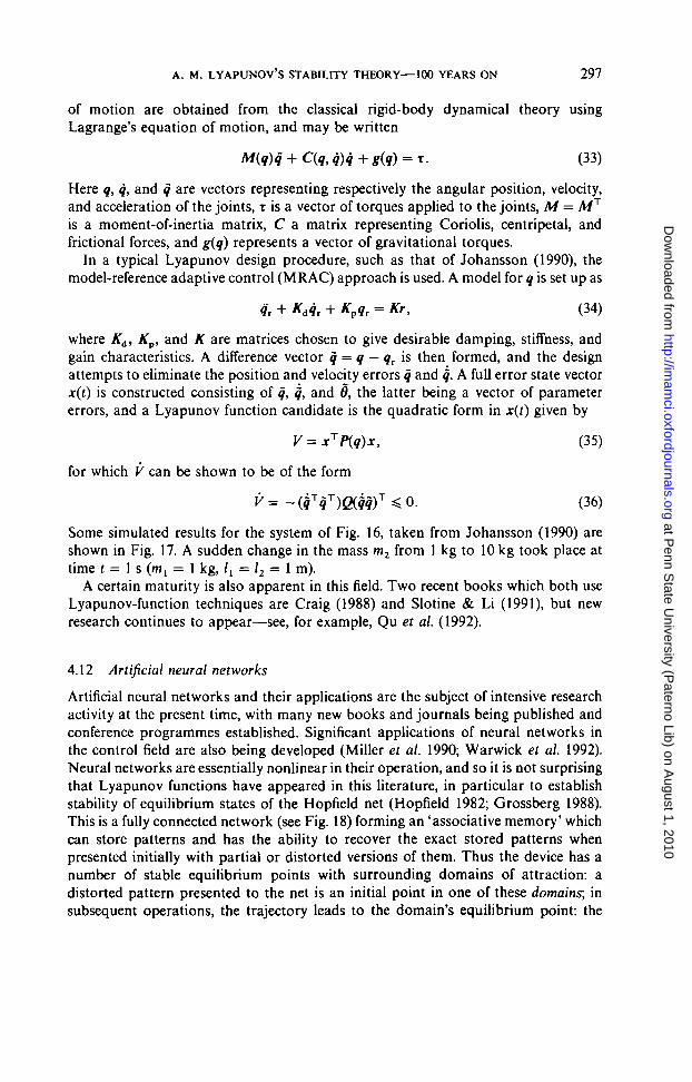
A. M. LYAPUNOV'S STABILITY THEORY—100 YEARS ON 297
of motion are obtained from the classical rigid-body dynamical theory usingLagrange's equation of motion, and may be written
M(q)q + C(q,q)q+g{q) = x. (33)
Here q, q, and q are vectors representing respectively the angular position, velocity,and acceleration of the joints, x is a vector of torques applied to the joints, M = MT
is a moment-of-inertia matrix, C a matrix representing Coriolis, centripetal, andfrictional forces, and g(q) represents a vector of gravitational torques.
In a typical Lyapunov design procedure, such as that of Johansson (1990), themodel-reference adaptive control (MRAC) approach is used. A model for q is set up as
q\ + Kdq, + Kpqr = Kr, (34)
where Kd, Kp, and K are matrices chosen to give desirable damping, stiffness, andgain characteristics. A difference vector q = q — qt is then formed, and the designattempts to eliminate the position and velocity errors q and q. A full error state vectorx(t) is constructed consisting of q, q, and S, the latter being a vector of parametererrors, and a Lyapunov function candidate is the quadratic form in x(t) given by
V=xTP{q)x, (35)
for which V can be shown to be of the form
i T <o. (36)
Some simulated results for the system of Fig. 16, taken from Johansson (1990) areshown in Fig. 17. A sudden change in the mass m2 from 1 kg to 10 kg took place attime t = 1 s (ml = 1 kg, /t = /2 = 1 m).
A certain maturity is also apparent in this field. Two recent books which both useLyapunov-function techniques are Craig (1988) and Slotine & Li (1991), but newresearch continues to appear—see, for example, Qu et al. (1992).
4.12 Artificial neural networks
Artificial neural networks and their applications are the subject of intensive researchactivity at the present time, with many new books and journals being published andconference programmes established. Significant applications of neural networks inthe control field are also being developed (Miller et al. 1990; Warwick et al. 1992).Neural networks are essentially nonlinear in their operation, and so it is not surprisingthat Lyapunov functions have appeared in this literature, in particular to establishstability of equilibrium states of the Hopfield net (Hopfield 1982; Grossberg 1988).This is a fully connected network (see Fig. 18) forming an 'associative memory' whichcan store patterns and has the ability to recover the exact stored patterns whenpresented initially with partial or distorted versions of them. Thus the device has anumber of stable equilibrium points with surrounding domains of attraction: adistorted pattern presented to the net is an initial point in one of these domains; insubsequent operations, the trajectory leads to the domain's equilibrium point: the
at Penn S
tate University (P
aterno Lib) on August 1, 2010
http://imam
ci.oxfordjournals.orgD
ownloaded from

298 P. C. PARKS
1-
-1
500-
-500-
10 20
L0 10
Estimated m^
20
10 20
400
L0 10
Lyapunov function
20
20
10-
0 —(—10
— I —
20
FIG. 17. Simulated results for the robot of Fig. 16.
fy-interconnection weights
FIG. 18. Hopfield net
exact stored pattern. The number of patterns that can be stored in this way appearsto be given approximately by O.\AN where N is the number of neurons in the network.
The input to node or neuron is Y,j li]xj + A. where tfJ are the 'weights' orinteractions between nodes, with ttj = tjt and tit = O, here xs are the outputs of thenodes and /, are the external inputs. The output xt from node i is given as x, = y, ifthe input is less than or equal to u(, and x, = v, if the input exceeds uh where v, > y,
at Penn S
tate University (P
aterno Lib) on August 1, 2010
http://imam
ci.oxfordjournals.orgD
ownloaded from

A. M. LYAPUNOV'S STABILITY THEORY—100 YEARS ON 299
and u, is the 'threshold' of neuron i. A Lyapunov-like function is given by
T Z (37)
where Tis the matrix with entries ttJ. Now the change in Kdue to a change AJC, in x, is
; (38)
here Ax, may be 0 or ±(u( — v,), where the sign is plus if Yj tuxj + /j — u( > 0 andminus if Yj hjxj + /( — "( < 0. Thus V can only decrease, and stability of the givenequilibrium point can be established.
The stability theory of control systems employing artificial neural networks hasyet to be developed. K. S. Narendra (Miller et al, 1990: p. 126) states that 'ourknowledge of the stability of dynamical adaptive systems using artificial neuralnetworks is quite rudimentary at the present time and considerable work remains tobe done . . . new concepts and methods based on stability theory will have to beexplored'. So far, only partial results are available, such as the proof of convergenceof the associative memory for the cerebellar model articulation controller (CMAC)of J. S. Albus (1975). This is given by Parks and Militzer (1989), where a rather trivialLyapunov function V = JCTX is employed. V is reduced as (discrete) time proceedsby an orthogonal projection algorithm for adjusting the 'weights' in the memory.The algorithm was originally invented by S. Kaczmarz (1937) for solving sets of linearalgebraic equations by iteration, and rediscovered by Albus.
Lyapunov-function arguments appear in a more decisive role in a recent paper byR. M. Sanner and J. J. E. Slotine (1991) which uses Gaussian radial basis functionsto compensate for plant nonlinearities and to develop a convergence weight-adjustment algorithm.
4.13 Other new concepts
A limited number of pages restricts discussion of many other current applications ofLyapunov's stability theory. One may note, however, the concept of'stability radius'developed in a series of papers on robustness of linear systems by D. Hinrichsen andA. J. Pritchard (1992) involving 'Lyapunov functions of maximum robustness'. Theauthors remark that they 'believe that this procedure (of going from matrices topolynomials) is both theoretically more productive and numerically more secure thanthe converse method, which tackles robustness problems for matrices by applyingpolynomial techniques (e.g. Kharitonov's theorem) to their characteristic poly-nomials'.
Another current application of Lyapunov stability theory is the proof of stabilityof so called 'receding-horizon control' of nonlinear systems developed by H.Michalska and D. Q. Mayne (1990, 1991) as the solution of a constrained optimalcontrol problem.
Finally, Lyapunov-like arguments are used by Brockett (1991a)—see also Brockett(1991b)—with the intriguing title 'Dynamical systems that sort lists, diagonalize
at Penn S
tate University (P
aterno Lib) on August 1, 2010
http://imam
ci.oxfordjournals.orgD
ownloaded from
300 P. C. PARKS
matrices, and solve linear programming problems'. This concerns equilibrium statesof the n x n matrix differential equation
H=H2N- 2HNH + NH2, (39)
where H is a real symmetric and N a real diagonal matrix. One remarkable propertyof the solution H(t) of (39) is that, if N is a diagonal matrix with differing elementsNn »•••> N*n> then H(co) is a diagonal matrix consisting of the eigenvalues of //(0)ordered according to the relative magnitudes of Nu ,..., NM.
5. Acknowledgements
The present author thanks the many correspondents, listed as follows, who sent himcopies of their papers and also useful comments on current and past applications ofLyapunov's stability theory: B. D. O. Anderson, S. Barnett, J. F. Barrett, C. C. Bissell,R. W. Brockett, P. A. Cook, A. T. Fuller, C. C. Hang, R. Johansson, P. V. Kokotovic,T. H. Lee, A. G. J. MacFarlane, I. M. Y. Mareels, D. Q. Mayne, H. Michalska,D. H. Owens, A. J. Pritchard, H. H. Rosenbrock, P. S. Shcherbakov, J. J. E. Slotine,T. Soderstrom, and C. Storey. Limitations of space have enabled only a small partof this material to be reported here. The historical account in Section 1 is based onmaterial prepared by J. F. Barrett (1992) and P. S. Shcherbakov (1992). It is a tributeto the memory of A. M. Lyapunov that today, 100 years after the publication hisdoctoral thesis of 1892, the ideas contained in it are in such widespread use in somany vital areas of modern technology.
REFERENCES
AIZERMAN, M. A. 1949 On a problem relating to the global stability of dynamic systems.Uspehi, Mat. Nauk. 4.
ALBUS, J. S. 1975 A new approach to manipulator control: the articulation controller (CMAC)ASME Trans. Ser. G (J. of Dynamics Systems, Measurement & Control) 97, 220-7.
ANDERSON, B. D. O. 1972 The reduced Hermite criterion with application to the proof of theLienard-Chipart criterion. IEEE Trans. AC 17, 669-72.
ANDERSON, B. D. O., BITMEAD, R. R., JOHNSON JR, C. R., KOKOTOVIC, P. V., KOSUT, R. L.,
MAREELS, I. M. Y., PRALY, L., & RIEDLE, B. D. 1986 Stability of adaptive systems: passivityand averaging analysis. M.l.T. Press, Cambridge, Mass.
ASTR6M, K. J., & WITTENMARK, B. 1989 Adaptive control. Addison-Wesley, Reading, Mass.BARNETT, S., & STOREY, C. 1967 Analysis and synthesis of stability matrices. J. Diffl. Eqns. 3,
414-22.BARNETT, S., & STOREY, C. 1988 Some results on the sensitivity and synthesis of asymptotically
stable linear and non-linear systems. Automatica 4, 187-94.BARRETT, J. F. (translator) 1992 Biography of A. M. Lyapunov by V. I. Smirnov. Int. J.
Control 55, 775-84.BROCKETT, R. W. 1964 On the stability of non-linear feedback systems. IEEE Trans. Applies
& Industry 83, 443-9.BROCKETT, R. W. 1970 Finite dimensional linear systems. Wiley, New York.BROCKETT, R. W. 1991a Dynamical systems that sort lists, diagonalise matrices and solve
programming problems. Linear algebra and its applications 146. Pp. 79-91.BROCKETT, R. W. 1991b An estimation theoretic basis for the design of sorting and
classification networks: theory and applications. In: Neural networks, theory and appli-cations (Mammone, R. J., & Zeevi, Y. Y., Eds). Academic Press, Boston. Pp. 23-41.
at Penn S
tate University (P
aterno Lib) on August 1, 2010
http://imam
ci.oxfordjournals.orgD
ownloaded from

A. M. LYAPUNOV'S STABILITY THEORY—100 YEARS ON 301
CHETAYEV, N. G. 1961 The stability of motion. Pergamon Press, Oxford.COOK, P. A. 1980 On the behaviour of dynamical systems subject to bounded disturbances.
Int. J. Systems Sci. 11, 159-70.CRAIG, J. J. 1988 Adaptive control of mechanical manipulators. Addison-Wesley, Reading, Mass.FULLER, A. T. 1992 Lyapunov Centenary Issue—Guest Editorial. Int. J. Control 55, 521-7.GERSHGORIN, S. 1931 Uber die Abgrenzung der Eigenwerte einer Matrix. Izv. Akad. Nauk SSSR
7, 749-54.GOODWIN, G. C , & SIN, K. S. 1984 Adaptive filtering, prediction and control. Prentice Hall,
Englewood Cliffs, NJ.GREGORY, P. C. (Ed.) 1959 Proceedings of the self-adaptive flight control systems symposium,
Wright Air Development Center, 1959.GROSSBERG, S. 1988 Non-linear neural networks: principles, mechanisms and architectures.
Neural Networks 1, 17-61.HERMITE, C. 1856 On the number of roots of an algebraic equation contained between given
limits. (English translation by P. C. Parks 1977). Int. J. Control 26, 183-95.HINRICHSEN, D., & PRITCHARD, A. J. 1992 Robustness measures for linear systems with
application to stability radii of Hurwitz and Schur polynomials. Int. J. Control 55,809-44.HOPFIELD, J. J. 1982 Neural networks and physical systems with emergent collective
computational abilities. Proc. Nat. Acad. Sci. 74, 2554-8.HURWITZ, A. 1895 Uber die Bedingungen unter welchen eine Gleichung nur Wurzeln mit
negativen reellen Teilen besitz. Math. Ann. 46, 273-84.INGWERSON, D. R. 1961 A modified Lyapunov method for non-linear stability analysis. IRE
Trans. AC 6, 199-210.JOHANSSON, R. 1990 Adaptive control of robot manipulator motion. IEEE Trans. AC 6,483-90.JURY, E. I. 1974 Inners and stability of dynamic systems. Wiley, New York.KACZMARZ, S. 1937 Angenaherte Auflosung von Systemen linearer Gleichungen. Bull. Int.
Polon. Acad. Sci. Cl. Math. Ser A, 355-7.KALMAN, R. E., & BERTRAM, J. E. 1960 Control system analysis and design via the second
method of Lyapunov. ASME Trans. D 82, 371-400.KALMAN, R. E. 1963. Lyapunov functions for the problem of Lur'e in automatic control. Proc.
Nat. Acad. Sci. 49, 201-5.KHARITONOV, V. L. 1978 Asymptotic stability of an equilibrium position of a family of systems
of linear differential equations. Differencial'nye Uravneniya 14, 2086-8.KRASOVSKII, N. N. 1963 Stability of motion. Stanford University Press.LANDAU, Y. D. 1979 Adaptive control—the model reference approach. Marcel Dekker, New
York.LEFSCHETZ, S., & LA SALLE, J. P. 1961 Stability of Lyapunov s direct method, with applications.
Academic Press, New York.LETOV, A. M. 1961 Stability in non-linear control systems (English translation). Princeton
University Press.LUR'E, A. I. 1957 Some non-linear problems in the theory of automatic control (English
translation). H.M.S.O., London.LYAPUNOV, A. M. 1884 On the stability of ellipsoidal forms of equilibrium of rotating fluids (in
Russian). Master's dissertation, University of St. Petersburg 1884. Republished in French,University of Toulouse, 1904.
LYAPUNOV, A. M. 1892 The general problem of the stability of motion (in Russian). KharkovMathematical Society (250 pp.), Collected Works II, 7. Republished by the University ofToulouse 1908 and Princeton University Press 1949 (in French), republished in Englishby Int. J. Control 1992—see the following reference.
LYAPUNOV, A. M. 1992 The general problem of the stability of motion (translated into Englishby A. T. Fuller). Int. J. Control 55, 531-773. Also published as a book by Taylor &Francis, London.
MACFARLANE, A. G. J. 1963 The calculation of functionals of the time and frequency responseof a linear constant coefficient dynamical system. Quart. J. Mech. & Appl. Math. 16,259-71.
at Penn S
tate University (P
aterno Lib) on August 1, 2010
http://imam
ci.oxfordjournals.orgD
ownloaded from

302 P. C. PARKS
MALKIN, I. G. 1952 Theory of the stability of motion. Gostckhizdat, Moscow.MANSOUR, M., & ANDERSON, B. D. O. 1992 Kharitonov's theorem and the second method of
Lyapunov. Proceedings of the Workshop on Robust Control and Stability, Ascona,Switzerland, April 1992.
MICHALSKA, H., & MAYNE, D. Q. 1990 Receding horizon control of non-linear systems. IEEETrans. AC 35, 814-24.
MICHALSKA, H., & MAYNE, D. Q. 1991 Receding horizon control of non-linear systems withoutdifferentiability of the optimal value function. Systems & Control Lett. 16, 123-30.
MILLER, W. T., SUTTON, R. S., & WERBOS, P. J. (Eds). 1990 Neural networks for control. M.I.T.Press, Cambridge, Mass. (2nd printing 1991).
MONOPOLI, R. V. 1974 Model reference adaptive control with an augmented error signal.IEEE Trans AC 19, 474-84.
MOVCHAN, A. A. 1959 On Lyapunov's direct method in problems of stability of elastic systems.Prik. Math, i Mekh. 23, 483-93.
NARENDRA, K. S., & ANNASWAMY, A. M. 1989 Stable adaptive systems. Prentice-Hall,Englewood Cliffs, NJ.
OSBURN, P. V., WHITAKER, H. P., & KEZER, A. 1961 New developments in the design ofadaptive control systems. Inst. Aeronautical Sciences Paper 61-39.
PARKS, P. C. 1964a Lyapunov and the Schur-Cohn stability criterion. IEEE Trans. AC 9,121.
PARKS, P. C. 1964b A new look at the Routh-Hurwitz problem using Lyapunov's secondmethod. Bull, de VAcad. Polon. des Sciences, Ser. des sciences techniques 12(6), 19-21.
PARKS, P. C. 1966 Lyapunov redesign of model reference adaptive control systems. IEEETrans. AC 11, 362-7.
PARKS, P. C. 1969 A Lyapunov function having the stability matrix of Hermite in its timederivative. Electron. Lett. 5, 608-9.
PARKS, P. C , & MILITZER, J. 1989 Convergence properties of associative memory storagefor learning control systems (English translation). Automation & Remote Control 50,254-86.
PARKS, P. C , & PRJTCHARD, A. J. 1969 On the construction and use of Lyapunov functionals.Proc. 4th World Congress of IFAC, Warsaw, Paper 20.5.
PARKS, P. C , & PRITCHARD, A. J. 1972 Stability analysis in structural dynamics usingLyapunov functionals. J. Sound & Vibration 25, 609-21.
PENROSE, R. 1989 The emperor's new mind. Oxford University Press 1989, Vintage Books 1990.Fig. 5.14.
POPOV, V. M. 1973 Hyperstability of control systems. Springer-Verlag, New York.Qu, Z., DAWSON, D. M., & DORSEY, J. F. 1992 Exponential stable trajectory following of
robotic manipulators under a class of adaptive controls. Automatica 28, 579-86.ROHRS, C. E., VALAVANI, L. S., ATHANS, M., & STEIN, G. 1985 Robustness of continuous time
adaptive control algorithms in the presence of unmodelled dynamics. IEEE Trans AC 30,881-9.
ROSENBROCK, H. H. 1963 A method of investigating stability. Proceedings of the 2nd WorldCongress of IFAC, Basle, 1963. Butterworths, London. Vol. 1, 590-2.
ROUTH, E. J. 1877 A treatise on the stability of a given state of motion, particularly steadymotion (Adams Prize Essay, University of Cambridge). Macmillan, London.
RUELLE, D. 1989 Chaotic evolution and strange attractors. Cambridge University Press. Fig.18 (after R. S. Shaw).
SANNER, R. M., & SLOTINE, J. J. E. 1991 Gaussian networks for direct adaptive control. Proc.1991 American Auto. Control Conference. Pp. 2153-9. (Also in IEEE Trans, on NeuralNetworks, 3, 837-63, 1992.)
SASTRY, S., & BODSON, M. 1989 Adaptive control: stability, convergence, robustness. Prentice-Hall, Englewood Cliffs, NJ.
SCHULTZ, D. G., & GIBSON, J. E. 1962 The variable gradient method for generating Lyapunovfunctions. Trans. AlEE Applies & Industry 81, 203-10.
SHCHERBAKOV, P. S. 1992 Alexander Mikhailovitch Lyapunov. Automatica 28, 865-71.
at Penn S
tate University (P
aterno Lib) on August 1, 2010
http://imam
ci.oxfordjournals.orgD
ownloaded from

A. M. LYAPUNOV'S STABILITY THEORY—100 YEARS ON 303
SLOTINE, J. J. E. 1988 Putting physics in control—the example of robotics. IEEE ControlSystems Mag. 8 (6), 12-18.
SLOTINE, J. J. E., & Li, W. 1987 On the adaptive control of robot manipulators. Int. J.Robotics Res. 6, 49-59.
SLOTINE, J. J. E., & Li, W. 1991 Applied non-linear control. Prentice-Hall, Englewood Cliffs, NJ.WARWICK, K., IRWIN, G. W., & HUNT, K. J. (Eds) 1992 Neural networks for control and
systems. Peter Peregrinus, London.ZUBOV, V. I. 1962 Mathematical methods for the study of automatic control systems. Pergamon
Press, Oxford.
at Penn S
tate University (P
aterno Lib) on August 1, 2010
http://imam
ci.oxfordjournals.orgD
ownloaded from