Embed Size (px)
Citation preview

A Local Convergence Analysis of
Bilevel Decomposition Algorithms
Victor DeMiguel Walter Murray
Decision Sciences Management Science and Engineering
London Business School Stanford University
[email protected] [email protected]
18th April 2004
Multidisciplinary design optimization (MDO) problems are engineering design problems that require the consid-
eration of the interaction between several design disciplines. Due to the organizational aspects of MDO problems,
decomposition algorithms are often the only feasible solution approach. Decomposition algorithms reformulate
the MDO problem as a set of independent subproblems, one per discipline, and a coordinating master problem.
A popular approach to MDO problems is bilevel decomposition algorithms. These algorithms use nonlinear opti-
mization techniques to solve both the master problem and the subproblems. In this paper, we propose two new
bilevel decomposition algorithms and analyze their properties. In particular, we show that the proposed problem
formulations are mathematically equivalent to the original problem and that the proposed algorithms converge lo-
cally at a superlinear rate. Our computational experiments illustrate the numerical performance of the algorithms.
Key words. Decomposition algorithms, bilevel programming, nonlinear programming, multidisciplinary design
optimization (MDO).
1 Introduction
Quoting Sobieszczanski-Sobieski and Haftka [19], Multidisciplinary Design Optimization (MDO) problems
may be defined as problems that
... involve the design of systems where the interaction between several disciplines must be
considered, and where the designer is free to significantly affect the system performance in
more than one discipline.
1

The interdisciplinary nature of MDO problems makes them challenging from both a computational and
an organizational perspective. From a computational perspective MDO problems integrate several dis-
ciplinary analysis, which usually require solving large-scale nonlinear problems. From an organizational
perspective, MDO problems usually require the participation of several persons within one or more orga-
nizations. Moreover, often different computer codes are used to perform each of the disciplinary analysis.
These are sophisticated codes that have been under development for many years and that are subject to
constant modification. As a result, it is often impractical to integrate all of the disciplinary codes into a
single hardware platform.
In this context, decomposition algorithms may be the only feasible alternative to finding the optimal
design. Decomposition algorithms exploit the structure of MDO problems by reformulating them as a
set of independent subproblems, one per discipline. Then, a so-called master problem is used to coordi-
nate the subproblem solutions and find an overall problem minimizer. For a detailed discussion of the
computational and organizational aspects of MDO problems see the monograph [1], the reviews [7, 19],
and the research articles [31, 28, 27, 26, 20].
A popular decomposition approach to MDO problems is bilevel decomposition algorithms. Once
decomposed into a master problem and a set of subproblems, the MDO is a particular type of bilevel
program [21, 29, 13]. Bilevel decomposition algorithms apply nonlinear optimization techniques to solve
both the master problem and the subproblems. At each iteration of the algorithm solving the master
problem, each of the subproblems is solved, and their minimizers used to compute the master problem
derivatives and their associated Newton direction.
Braun [4] proposed a bilevel decomposition algorithm known as Collaborative Optimization (CO). The
algorithm uses an inexact (quadratic) penalty function to decompose the MDO problem. Unfortunately,
it is easy to show that both the CO master problem and subproblems are degenerate [9]. Nondegeneracy is
a common assumption when proving convergence for most optimization algorithms. Not surprisingly, CO
fails to converge on some simple test problems even when the starting point is very close to the minimizer
[3]. Moreover, some convergence difficulties have been observed in the application of the algorithm to
some simplified real-world problems [5, 30, 22].
In this paper, we propose two bilevel decomposition algorithms closely related to CO that overcome
some of the difficulties associated with CO. The first algorithm is termed Inexact Penalty Decomposition
(IPD) and uses an inexact penalty function. The second algorithm is termed Exact Penalty Decomposition
(EPD) and employs an exact penalty function in conjunction with a barrier term. We analyze the local
convergence properties of the proposed algorithms. The relevance of our analysis is twofold. Firstly, we
show that the proposed problem formulations are mathematically equivalent to the original MDO problem.
That is, under mild assumptions, KKT points of the MDO problem are KKT points of the decomposed
problem and vice versa. Secondly, we show that the proposed master problem and subproblems are
2

nondegenerate. Consequently, we can show that standard nonlinear programming algorithms converge
locally at a fast rate when applied to solve the proposed mater problem and subproblems.
The remainder of this paper is organized as follows. In Section 2, we give the mathematical statement
of the MDO problem. In Section 3, we describe collaborative optimization and point out its difficulties.
In Section 4, we introduce IPD and analyze its local convergence properties. Section 5 is devoted to EPD.
Finally, we show the results of our computational experiments in Section 6.
2 Problem Statement
To simplify our analysis, herein we consider a special type of MDO problem termed quasi-separable MDO
problem [20]. The term quasi-separable refers to the fact that the objective function terms and constraints
of each of the different systems are only coupled through a few of the variables, which we term global
variables. This problem is general enough to cover many engineering design problems, yet simple enough
to allow for rigorous analysis. The quasi-separable MDO problem may be stated as follows:
minx,y1,...,yN
F1(x, y1) + F2(x, y2) + . . .+ FN (x, yN )
s.t. c1(x, y1) ≥ 0
c2(x, y2) ≥ 0...
cN (x, yN ) ≥ 0,
(1)
where x ∈ Rn are the global variables, yi ∈ Rni are the ith system local variables, ci : Rn ×Rni → Rmi
are the ith system constraints, and Fi : Rn ×Rni → R is the objective function term corresponding to
the ith system. Note that while global variables appear in all of the constraints and objective function
terms, local variables only appear in the objective function term and constraints corresponding to one of
the systems. Herein, we refer to problem (1) as the MDO problem.
3 Decomposition Algorithms
The structure of the MDO problem suggests it may be advantageously broken into N independent
subproblems, one per system. In this section, we explain how a CO-like bilevel decomposition algorithm
may be applied to problem (1).
3

3.1 Bilevel Decomposition Algorithms
A bilevel decomposition algorithm divides the job of finding a minimizer to problem (1) into two different
tasks: (i) finding an optimal value of the local variables (y∗1(x), y∗2(x), . . . , y∗N (x)) for a given value of the
global variables x, and (ii) finding an overall optimal value of the global variables x∗. The first task is
performed by solving N subproblems. Then the subproblem solutions are used to define a master problem
whose solution accomplishes the second task.
There are several types of bilevel decomposition algorithms. For expositional purposes, we consider a
bilevel decomposition algorithm that is a close relative of collaborative optimization. The algorithm may
be described as follows. Solve the following master problem:
minx
F ∗
1 (x) + F ∗
2 (x) + · · · + F ∗
N (x),
where F ∗
i (x) = Fi(x, y∗
i (x)) for i = 1 : N are the subproblem optimal value functions
F ∗
1 (x) = miny1
F1(x, y1)
s.t. c1(x, y1) ≥ 0· · ·
F ∗
N (x) = minyN
FN (x, yN )
s.t. cN (x, yN ) ≥ 0.
Note that the global variables are just a parameter within each of the subproblems defined above.
Consequently, the subproblems are independent from each other and may be solved in parallel. Moreover,
the master problem only depends on the global variables. Thus, the above formulation allows the different
disciplines to be dealt with almost independently, and only a limited amount of information regarding
the global variables is exchanged between the master problem and the subproblems.
Roughly speaking, a bilevel decomposition algorithm applies a nonlinear optimization method to solve
the master problem. At each iteration, a new estimate of the global variables xk is generated and each of
the subproblems is solved using xk as a parameter. Then, sensitivity analysis formulae [15] are used to
compute the master problem objective and its derivatives from the subproblem minimizers. Using this
information, a new estimate of the global variables xk+1 is computed. This procedure is repeated until a
master problem minimizer is found.
Tammer [32] shows that the general bilevel programming approach stated above converges locally at
a superlinear rate assuming that the MDO minimizer satisfies the so-called strong linear independence
constraint qualification; that is, assuming that at the minimizer (x, y1, . . . , yN ), the vectors ∇yici(x, yi)
corresponding to the active constraints are linearly independent. Roughly speaking, the SLICQ implies
that for any value of the global variables in a neighborhood of x, there exist values of the local variables
for which all of the constraints are satisfied. As the name implies this is a restrictive assumption and
is in a sense equivalent to assuming (at least locally) that the problem is an unconstrained one in the
4

global variables only. DeMiguel and Nogales [12] propose a bilevel decomposition algorithm based on
interior-point techniques that also converges superlinearly under the SLICQ.
But in this paper we focus on the case where only the weaker (and more realistic) linear indepen-
dence constraint qualification (LICQ) holds; that is, the case where the gradients ∇x,y1,...,yNci(x, yi)
corresponding to the active constraints are linearly independent. In this case, a major difficulty in the
general bilevel programming approach stated above is that the algorithm breaks down whenever one of
the subproblems is infeasible at one of the master problem iterates. In particular, the algorithm will fail
if for a given master problem iterate xk and for at least one of the systems j ∈ {1, 2, . . . , N}, there does
not exist yj such that cj(xk, yj) ≥ 0. Unlike when SLICQ holds, when only LICQ holds this difficulty
may arise even when the iterates are in the vicinity of the minimizer.
3.2 Collaborative Optimization (CO)
To overcome this difficulty, Braun [4] proposed a bilevel decomposition algorithm for which the subprob-
lems are always feasible, provided the original MDO problem is feasible. To do so, Braun allows the
global variables to take a different value xi within each of the subproblems. Then, the global variables for
all systems (xi for i = 1 : N) are forced to converge to the same value (given by the target variable vector
z) by using quadratic penalty functions. Several CO formulations have been considered in the literature
[4, 5, 2]. To simplify the exposition we consider the following CO formulation. Solve the following master
problem
minz
∑N
i=1 Fi(z, yi)
s.t. p∗i (z) = 0, i = 1:N,
where p∗i (z) for i = 1 : N are the ith subproblem optimal-value functions:
p∗1(z) = minx1,y1
‖x1 − z‖22
s.t. c1(x1, y1) ≥ 0.· · ·
p∗N (z) = minxN ,yN
‖xN − z‖22
s.t. cN (xN , yN ) ≥ 0,
where yi and ci and Fi are as defined in (1), the global variables x1, x2, . . . , xN ∈ Rn, and the target
variables z ∈ Rn. Note that, at a solution z∗ to the master problem, p∗i (z∗) = 0 and therefore x∗i = z∗
for i = 1:N .
The main advantage of CO is that, provided problem (1) is feasible, the subproblems are feasible.
Unfortunately, it is easy to show that its master problem and the subproblems are degenerate; that is, their
minimizer does not satisfy the linear independence constraint qualification, the strict complementarity
slackness conditions, and the second order sufficient conditions (see Appendix A for a definition of these
nondegeneracy conditions). The degeneracy of the subproblems is easily deduced from the form of the
5

subproblem objective gradient:
∇xi,yi‖xi − z‖2
2 =
2(xi − z)
0
.
At the solution, x∗i = z∗ and therefore the subproblem objective gradient is zero. Given that the
original problem (1) satisfies the linear independence constraint qualification, this in turn implies that the
subproblem Lagrange multipliers are zero and therefore the strict complementarity slackness conditions
do not hold at the subproblem minimizer. Thus, the subproblems are degenerate at the solution.
Moreover, the degeneracy of the subproblems implies that the optimal-value functions p∗i (z) are not
smooth in general [15, Theorem 12] and thus the master problem is a nonsmooth optimization problem.
Nondegeneracy and smoothness are common assumptions when proving local convergence for most opti-
mization algorithms [23]. In fact, Alexandrov and Lewis [3] give a linear and a quadratic programming
problem on which CO failed to converge to a minimizer even from starting points close to a minimizer.
4 Inexact Penalty Decomposition
In this section, we propose a decomposition algorithm closely related to collaborative optimization. Like
CO, our algorithm makes use of an inexact (quadratic) penalty function. Our formulation, however, over-
comes the principle difficulties associated with CO. We term the algorithm Inexact Penalty Decomposition
(IPD).
This section is organized as follows. In Section 4.1, we state the proposed master problem and
subproblems. In Section 4.2, we describe the optimization algorithms used to solve the master problem
and the subproblems. In Section 4.3, we analyze the properties of IPD. The relevance of our analysis
is twofold. Firstly, we show that under mild conditions the MDO problem and the IPD formulation
are mathematically equivalent. That is, KKT points of the MDO problem are KKT points of the IPD
formulation and vice versa. Secondly, we show that under standard nondegeneracy assumptions on
the MDO minimizer, the IPD master problem and subproblems are also nondegenerate. Using these
nondegeneracy results, we show in Section 4.4 that the optimization algorithms used to solve the master
problem and the subproblems converge locally at a superlinear rate for each value of the penalty parameter.
4.1 Problem Formulation
Our formulation shares two features with collaborative optimization: (i) it allows the global variables
to take a different value within each of the subproblems, and (ii) it uses quadratic penalty functions to
force the global variables to asymptotically converge to the target variables. However, unlike CO, our
formulation explicitly includes a penalty parameter γ that allows control over the speed at which the
6

global variables converge to the target variables. In particular, we propose solving the following master
problem for a sequence of penalty parameters {γk} such that γk → ∞:
minz
N∑
i=1
F ∗
i (γk, z), (2)
where F ∗
i (γk, z) is the ith subproblem optimal-value function,
F ∗
i (γk, z) = minxi,yi
Fi(xi, yi) + γk‖xi − z‖22
s.t. ci(xi, yi) ≥ 0,(3)
Fi, ci, and yi are as in problem (1), xi ∈ Rn are the ith system global variables, and z ∈ Rn are the
target variables. Note that, because quadratic penalty functions are inexact for any finite value of γk, we
have to solve the above master problem for a sequence of penalty parameters {γk} such that γk → ∞ in
order to recover the exact solution x∗i = z∗. Finally, to simplify notation, herein we omit the dependence
of the subproblem optimal value function on the penalty parameter; thus we refer to F ∗
i (γk, z) as F ∗
i (z).
Note that, unlike CO, IPD uses the subproblem optimal-value functions F ∗
i (z) as penalty terms within
the objective function of an unconstrained master problem. In CO, constraints are included in the master
problem setting the penalty functions to zero. In essence, this is equivalent to an IPD approach in which
the penalty parameter is set to a very large value from the very beginning. In contrast, IPD allows the
user to drive the penalty parameter to infinity gradually. This is essential to the development of a suitable
convergence theory.
4.2 Algorithm Statement
In the previous section, we proposed solving the sequence of master problems corresponding to a sequence
of increasing penalty parameters {γk}. To illustrate the behavior of the algorithm, we need to specify how
to solve the master problem and subproblems. In practice a variety of methods could be used to solve
these problems. However, here we use a BFGS quasi-Newton method [18, 16] to solve the master problem.
These methods use the objective function gradient to progressively build a better approximation of the
Hessian matrix. At each iteration, the quasi-Newton method generates a new estimate of the target
variables zk. Then, all of the subproblems are solved with z = zk and the master problem objective
and its gradient are computed from the subproblem minimizers. Using this information, the master
problem Hessian is updated and a new estimate of the target variables zk+1 is generated. This procedure
is repeated until a master problem minimizer is found. To solve the subproblems we use the sequential
quadratic programming (SQP) algorithm NPSOL [17].
The master problem objective and its gradient can e computed from the subproblem from the subprob-
7

lem minimizers. In particular, the master problem objective F ∗(z) can be evaluated at the subproblem
solution (xi(z), yi(z)) as
F ∗(z) =N∑
i=1
F ∗
i (z) =N∑
i=1
[Fi(xi(z), yi(z)) + γ‖xi(z) − z‖22]. (4)
Moreover, in Section 4.3 we will show that, provided z is close to the master problem minimizer z∗,
the subproblem minimizers satisfy the nondegeneracy conditions A.1-A.3. This implies [15, Theorem
6] that the master problem objective is differentiable. Furthermore, it is easy to compute the master
problem gradient ∇zF∗(z) from the subproblem minimizer. To see this, note that by the complementarity
conditions we have that
F ∗
i (z) = Fi(xi(z), yi(z)) + γ‖xi(z) − z‖22 = Li(xi(z), yi(z), λi(z), z),
where Li is the ith subproblem Lagrangian function, (xi(z), yi(z)) is the minimizer to the ith subproblem
as a function of z, and λi(z) are the corresponding Lagrange multipliers. Then applying the chain rule
we have that
dLi(xi(z), yi(z), λi(z), z)
dz= ∇xi
Li(xi(z), yi(z), λi(z), z) x′
i(z) (5)
+ ∇yiLi(xi(z), yi(z), λi(z), z) y
′
i(z) (6)
+ ∇λiLi(xi(z), yi(z), λi(z), z) λ
′
i(z), (7)
+ ∇zLi(xi(z), yi(z), λi(z), z), (8)
where x′i(z), y′
i(z), λ′
i(z) denote the Jacobian matrices of xi(z), yi(z), λi(z) evaluated at z. Note that
(5) and (6) are zero because of the optimality of (xi(z), yi(z)), (7) is zero by the feasibility and strict
complementarity slackness of (xi(z), yi(z)), and ∇zLi(xi(z), yi(z), λi(z), z) = −2γ(xi(z) − z). Thus, we
can write the master problem objective gradient as
∇F ∗(zk) =
N∑
i=1
∇F ∗
i (zk) = −2γ
N∑
i=1
(xik − zk). (9)
The resulting decomposition algorithm is outlined in Figure 1.
Note that the penalty parameter is increased in Step 1 until the global variables are close enough to
the target variables; that is, until∑N
i=1 ‖xik − zk‖22/(1 + ‖zk‖) < ǫ, where ǫ is the optimality tolerance.
Note also that, for each value of the penalty parameter, the master problem is solved using a BFGS
quasi-Newton method (Step 2). Finally, in order to compute the master problem objective function with
the precision necessary to ensure fast local convergence, a tight optimality tolerance must be used to
8

Initialization: Initialize γ and set the iteration counter k := 0. Choose astarting point z0. For i = 1 : N , call NPSOL to find the subproblem minimizers(xi0, yi0). Set the initial Hessian approximation B0 equal to the identity. Chooseσ ∈ (0, 1).
while (PN
i=1‖xik − zk‖
22/(1 + ‖zk‖) > ǫ)
1. Penalty parameter update: increase γ.
2. Solve master problem with current γ:repeat
(a) Function evaluation: for i = 1 : N call NPSOL with γ and computeF ∗(zk) and ∇F ∗(zk) from (4) and (9).
(b) Search direction: Solve Bk∆z = −∇F ∗(zk).
(c) Backtracking line search:α := 1.while (F ∗(zk + α∆z) − F ∗(zk) > σ∇F ∗(zk)T ∆z)
α := α/2. Call NPSOL to evaluate F ∗(zk + α∆z).endwhiles := α∆z, y := ∇F ∗(zk + s) −∇F ∗(zk).zk+1 := zk + s.
(d) BFGS Hessian update: Bk+1 := Bk − BkssT Bk
sT Bks+ yyT
yT s
(e) k = k+1.
until (‖∇F ∗(zk)‖/|1 + F ∗(zk)| < ǫ)
endwhile
Figure 1: Inexact penalty decomposition
solve the subproblems with NPSOL. In our implementation, we use a subproblem optimality tolerance
of ǫ2, where ǫ is the optimality tolerance used to solve the master problem.
4.3 Mathematical Equivalence and Nondegeneracy
In this section we analyze the theoretical properties of IPD. In particular, we show that, given a nonde-
generate MDO minimizer (that is, given an MDO minimizer satisfying the linear independence constraint
qualification, the strict complementarity slackness conditions, and the second order sufficient conditions;
see Appendix A), there exists an equivalent trajectory of minimizers to the IPD master problem and
subproblems that are also nondegenerate. Conversely, we show that, under mild conditions, an accumu-
lation point of IPD nondegenerate local minimizers, is a KKT point for the MDO problem. The result is
summarized in Theorems 4.10 and 4.11.
The importance of this result is twofold. Firstly, our analysis implies that under mild conditions the
MDO problem and the proposed IPD formulation are mathematically equivalent. That is, nondegenerate
KKT points of the MDO problem are nondegenerate KKT points of the IPD formulation and vice versa.
Secondly, the nondegeneracy of the equivalent IPD minimizers implies that Newton-like algorithms will
9

converge locally at a fast rate when applied to solve the IPD formulation.
To prove the result, it is essential to realize that the proposed master problem and subproblems can
be derived from the MDO problem through a sequence of three manipulations: (i) introduction of the
target variables, (ii) introduction of an inexact penalty function, and (iii) decomposition. The result can
be shown by realizing that mathematical equivalence and nondegeneracy are preserved by each of these
transformations.
The remainder of this section is organized as follows. In Section 4.3.1 we discuss the assumptions
and some useful notation. In Sections 4.3.2, 4.3.3, and 4.3.4 we establish that mathematical equivalence
and nondegeneracy of a local minimizer is preserved by each of the three transformations listed above.
Finally, in Section 4.3.5, we give two theorems summarizing the result.
In Section 4.4, we use the nondegeneracy results to prove that the algorithms proposed to solve the
master problem and the subproblems converge superlinearly for each value of the penalty parameter.
4.3.1 Notation and assumptions
To simplify notation and without loss of generality, herein we consider the MDO problem composed of
only two systems. The interested reader is referred to [8, 11] for an exposition with N systems. The
MDO problem with two systems is:
minx,y1,y2
F1(x, y1) + F2(x, y2)
s.t. c1(x, y1) ≥ 0,
c2(x, y2) ≥ 0,
(10)
where all functions and variables are as defined in (1).
We assume there exists a minimizer (x∗, y∗1 , y∗
2) and an associated Lagrange multiplier vector (λ∗1, λ∗
2)
satisfying the KKT conditions for problem (10). In addition, we assume that the functions in problem
(10) are three times continuously-differentiable in an open convex set containing w∗. Moreover, we assume
that the KKT point w∗ = (x∗, y∗1 , y∗
2 , λ∗
1, λ∗
2) is nondegenerate; that is, the linear independence constraint
qualification A.1, the strict complementarity slackness conditions A.2, and the second order sufficient
conditions A.3 hold at w∗; see Appendix A for a definition of the nondegeneracy conditions A.1-A.3.
Note that unlike the analysis in [32, 12] we only assume the LICQ and not the SLICQ holds at the MDO
minimizer.
10

4.3.2 Introducing target variables
The first manipulation applied to the MDO problem on our way to the proposed master problem is the
introduction of the target variable vector z ∈ Rn. The result is the following problem:
minx1,x2,y1,y2,z
2∑
i=1
Fi(xi, yi)
s.t. ci(xi, yi) ≥ 0, i = 1 : 2,
xi − z = 0, i = 1 : 2.
(11)
The following theorem shows that, given a nondegenerate MDO minimizer, there is an equivalent
minimizer to problem (11) that is also nondegenerate and vice versa.
Herein we denote the Jacobian matrix of the system constraints ci(x, yi) as the matrix ∇ci(x, yi) ∈Rmi×(n+ni) whose mi rows contain the gradients of the individual constraints cij(x, yi) for j = 1 : mi.
Theorem 4.1 A point (x, y1, y2) is a minimizer to problem (10) satisfying the nondegeneracy conditions
A.1-A.3 with the Lagrange multiplier vector (λ1, λ2) iff the point (x1, x2, y1, y2, z) with x1, x2, and z equal
to x is a minimizer to problem (11) satisfying the nondegeneracy conditions A.1-A.3 with the Lagrange
multiplier vector
λ1
λ2
∇xF1(x, y1) − (∇xc1(x, y1))Tλ1
∇xF2(x, y2) − (∇xc2(x, y2))Tλ2
. (12)
Proof: First we prove that the linear independence constraint qualification A.1 holds at a point (x, y1, y2)
for problem (10) iff it holds at (x1, x2, y1, y2, z) with x1, x2, and z equal to x for problem (11). To see
this, suppose that condition A.1 does not hold for problem (10). Thus, there exists (ψ1, ψ2) 6= 0 such
that
(∇xc1(x, y1))T (∇xc2(x, y2))
T
(∇y1c1(x, y1))
T
(∇y2c2(x, y2))
T
(
ψ1
ψ2
)
= 0, (13)
where c are the constraints active at (x, y1, y2). Then it is easy to see that
(∇xc1(x, y1))T I
(∇xc2(x, y2))T I
(∇y1c1(x, y1))
T
(∇y2c2(x, y2))
T
−I −I
ψ1
ψ2
ψ3
ψ4
= 0, (14)
11

with ψ3 = −(∇xc1(x, y1))Tψ1 and ψ4 = −(∇xc2(x, y2))
Tψ2. Thus, condition A.1 does not hold for
problem (11). Conversely, assume there exists (ψ1, ψ2, ψ3, ψ4) 6= 0 such that equation (14) holds. Then,
by the first and second rows in (14) we know that ψ3 = −(∇xc1(x, y1))Tψ1 and ψ4 = −(∇xc2(x, y2))
Tψ2.
Then by the third, fourth, and fifth rows in (14) it follows that equation (13) holds for (ψ1, ψ2).
Now we turn to proving that (x, y1, y2) satisfies the KKT conditions with the Lagrange multiplier
vector (λ1, λ2) for problem (10) iff (x1, x2, y1, y2, z) with x1, x2, and z equal to x satisfies the KKT
conditions with the Lagrange multiplier vector given by (12) for problem (11). First, note that obviously
the feasibility conditions (47)–(48) are satisfied at (x, y1, y2) for problem (10) iff they are satisfied at
(x1, x2, y1, y2, z) with x1, x2, and z equal to x for problem (11). Moreover, assume there exists (λ1, λ2) ≥ 0
satisfying the complementarity condition (49) at (x, y1, y2) such that
∑2i=1 ∇xFi(x, yi)
∇y1F1(x, y1)
∇y2F2(x, y2)
=
(∇xc1(x, y1))T (∇xc2(x, y2))
T
(∇y1c1(x, y1))
T
(∇y2c2(x, y2))
T
(
λ1
λ2
)
. (15)
Then we obviously have that
∇xF1(x, y1)
∇xF2(x, y2)
∇y1F1(x, y1)
∇y2F2(x, y2)
0
=
(∇xc1(x, y1))T I
(∇xc2(x, y2))T I
(∇y1c1(x, y1))
T
(∇y2c2(x, y2))
T
−I −I
λ, (16)
with λ as given by (12). Conversely, if there exists (λ1, λ2, λ3, λ4) satisfying equation (16), then by the
first and second rows in (16) we know that λ3 = ∇xF1(x, y1)− (∇xc1(x, y1))Tλ1 and λ4 = ∇xF2(x, y2)−
(∇xc2(x, y2))Tλ2. Then, by the third, fourth, and fifth rows in (16) we know that equation (15) is satisfied
at (x, y1, y2) with Lagrange multipliers (λ1, λ2). Furthermore, it is clear that the complementarity and
nonnegativity conditions (49) and (50) hold at (x, y1, y2) for problem (10) with (λ1, λ2) iff they hold at
(x1, x2, y1, y2, z) with x1, x2, and z equal to x for problem (11) with the Lagrange multiplier given by
(12).
To see that the strict complementarity slackness conditions A.2 hold at (x, y1, y2) for problem (10)
with (λ1, λ2) iff they hold at (x1, x2, y1, y2, z) with x1, x2, and z equal to x for problem (11) with
the Lagrange multiplier given by (12), simply note that the Lagrange multipliers associated with the
inequality constraints are the same for both problems (λ1, λ2).
It only remains to show that the second order sufficient conditions for optimality A.3 hold at (x, y1, y2)
for problem (10) with (λ1, λ2) iff they hold at (x1, x2, y1, y2, z) with x1, x2, and z equal to x for problem
(11) with the Lagrange multiplier given by (12). To prove this, we first note that there is a one-to-one
correspondence between the vectors tangent to the inequality constraints active at (x, y1, y2) for problem
(10) and the vectors tangent to the equality and inequality constraints active at (x1, x2, y1, y2, z) with
12

x1, x2, and z equal to x for problem (11). In particular, given τ1 = (τx, τy1, τy2
) such that
(
∇xc1(x, y1) ∇y1c1(x, y1)
∇xc2(x, y2) ∇y2c2(x, y2)
)
τ1 = 0, (17)
where c are the inequalities active at (x, y1, y2), we know that τ2 = (τx1, τx2
, τy1, τy2
, τz) with τx1, τx2
,
and τz equal to τx satisfies
∇xc1(x, y1) ∇y1c1(x, y1)
∇xc2(x, y2) ∇y2c2(x, y2)
I −I
I −I
τ2 = 0. (18)
Conversely, if τ2 = (τx1, τx2
, τy1, τy2
, τz) satisfies (18), then we know that τx1and τx2
are equal
to τz and that τ1 = (τx, τy1, τy2
) with τx = τz satisfies (17). Finally, given τ1 = (τx, τy1, τy2
) and
τ2 = (τx1, τx2
, τy1, τy2
, τz) with τx1, τx2
, and τz equal to τx, it is easy to see from the form of problems
(10) and (11) that τT1 ∇2L1τ1 = τT
2 ∇2L2τ2, where ∇2L1 is the Hessian of the Lagrangian for problem
(10) evaluated at (x, y1, y2, λ1, λ2), and ∇2L2 is the Hessian of the Lagrangian for problem (11) evaluated
at (x1, x2, y1, y2, z, λ) with λ as given by (12) and x1, x2 and z equal to x. �
4.3.3 Introducing an inexact penalty function
The second transformation operated on problem (10) in order to obtain the desired master problem is the
introduction of an inexact penalty function. We use a quadratic penalty function to remove the equality
constraints in problem (11) to derive the following problem:
minx1,x2,y1,y2,z
2∑
i=1
[Fi(xi, yi) + γ‖xi − z‖22]
s.t. ci(xi, yi) ≥ 0 i = 1 : 2.
(19)
The quadratic penalty functions has been extensively analyzed in the nonlinear optimization literature.
The following two theorems follow from standard results (see [15, 24]) and establish the mathematical
equivalence of problems (11) and (19). The first theorem follows from Theorems 14 and 17 in [15] and
shows that, given a nondegenerate minimizer to problem (11), there exists a trajectory of nondegenerate
minimizers to (19) that converge to it.
Theorem 4.2 If (x1, x2, y1, y2, z) is a minimizer satisfying the nondegeneracy conditions A.1-A.3 for
problem (11), then for γ sufficiently large, there exists a locally unique once continuously-differentiable
trajectory of points (x1(γ), x2(γ), y1(γ), y2(γ), z(γ)) satisfying the nondegeneracy conditions A.1-A.3 for
problem (19) such that limγ→∞(x1(γ), x2(γ), y1(γ), y2(γ), z(γ)) = (x1, x2, y1, y2, z).
The second theorem follows from Theorem 17.2 in [15] and shows that, under mild assumptions, any
13

accumulation point of nondegenerate local minimizers to problem (19) is a KKT point of problem (11).
To state the theorem we need to introduce some notation. We denote by ci(x∗
i , y∗
i ) the constraints that
are active at (x∗i , y∗
i ). That is, ci(x∗
i , y∗
i ) is the subset of the constraints ci(xi, yi) for which ci(x∗
i , y∗
i ) = 0.
Theorem 4.3 Let {(x1, x2, y1, y2, z)}k be a sequence of KKT points for problem (19) at which condition
A.1 holds and corresponding to a sequence of penalty parameters {γ}k with limk→∞ γk = ∞. Then, any
limit point (x∗1, x∗
2, y∗
1 , y∗
2 , z∗) of the sequence {(x1, x2, y1, y2, z)}k at which the gradients of the equality
constraints x∗1 = z∗, x∗2 = z∗ and the gradients of the active inequality constraints c1(x∗
1, y∗
1), c2(x∗
2, y∗
1)
are linearly independent is a KKT point of problem (11) at which condition A.1 holds.
4.3.4 Decomposition
We now consider the third transformation operated on the MDO problem. Note that problem (19) can
be decomposed into N independent subproblems by simply setting the target variables to a fixed value.
The subproblem optimal-value functions can then be used to define a master problem. The result is the
IPD formulation. Namely, solve the following master problem
minz
2∑
i=1
F ∗
i (z), (20)
where F ∗
i (z) is the ith subproblem optimal-value function
F ∗
i (z) = minxi,yi
Fi(xi, yi) + γ‖xi − z‖22
s.t. ci(xi, yi) ≥ 0.(21)
In this section, we show that problems (19) and (20)-(21) are mathematically equivalent. First, we
introduce some useful definitions.
Definition 4.4 A vector (x∗1, x∗
2, y∗
1 , y∗
2 , z∗) is a semi-local minimizer to problem (20) if for i = 1, 2 the
vector (x∗i , y∗
i ) is a local minimizer for the ith subproblem (21) with z = z∗.
Definition 4.5 A vector (x∗1, x∗
2, y∗
1 , y∗
2 , z∗) is a strict local minimizer to problem (20) if: (i) (x∗1, x
∗
2, y∗
1 , y∗
2 , z∗)
is a semi-local minimizer to problem (20), and (ii) there exists a neighborhood Nǫ(x∗
1, x∗
2, y∗
1 , y∗
2 , z∗) such
that if (x1, x2, y1, y2, z) lying in Nǫ is a semi-local minimizer then∑2
i=1[Fi(x∗
i , y∗
i ) + γ‖x∗i − z∗‖22] <
∑2i=1[Fi(xi, yi) + γ‖xi − z‖2
2].
The following lemma shows that a nondegenerate minimizer to problem (19) is also a strict local
minimizer to problem (20).
14
Lemma 4.6 If (x∗1, x∗
2, y∗
1 , y∗
2 , z∗) is a minimizer to problem (19) satisfying the second order sufficient
conditions A.3, then (x∗1, x∗
2, y∗
1 , y∗
2 , z∗) is also a strict local minimizer to problem (20).
Proof: We need to show that conditions (i) and (ii) in Definition 4.5 hold at (x∗1, x∗
2, y∗
1 , y∗
2 , z∗). Assume
(x∗1, x∗
2, y∗
1 , y∗
2 , z∗) is a minimizer to problem (19) satisfying condition A.3. Then, there exists a neighbor-
hood Nǫ(x∗
1, x∗
2, y∗
1 , y∗
2 , z∗) such that for all points (x1, x2, y1, y2, z) feasible with respect to problem (19)
and lying in Nǫ(x∗
1, x∗
2, y∗
1 , y∗
2 , z∗) we have that,
2∑
i=1
[Fi(x∗
i , y∗
i ) + γ‖x∗i − z∗‖22] <
2∑
i=1
[Fi(xi, yi) + γ‖xi − z‖22]. (22)
In particular, for all (x1, y1) such that ‖(x∗1, y∗
1)− (x1, y1)‖2 < ǫ we know by (22) that F1(x∗
1, y∗
1)+γ‖x∗1 −
z∗‖22 ≤ F1(x1, y1)+γ‖x1−z
∗‖22. Likewise, for all (x2, y2) such that ‖(x∗2, y
∗
2)−(x2, y2)‖2 < ǫ we know that
F2(x∗
2, y∗
2) + γ‖x∗2 − z∗‖22 ≤ F2(x2, y2) + γ‖x2 − z∗‖2
2. Thus, (x∗1, x∗
2, y∗
1 , y∗
2 , z∗) is a semi-local minimizer
to problem (20); i.e., condition (i) in Definition 4.5 holds. Also, every semi-local minimizer is feasible
with respect to problem (19). Therefore, by (22), we know that (x∗1, x∗
2, y∗
1 , y∗
2 , z∗) satisfies condition (ii)
in Definition 4.5. �
Moreover, in the following two theorems we show that the proposed subproblems and master problem
are nondegenerate.
Theorem 4.7 If (x∗1, x∗
2, y∗
1 , y∗
2 , z∗) is a minimizer satisfying the nondegeneracy conditions A.1-A.3 for
problem (19), then (x∗i , y∗
i ) is a minimizer satisfying the nondegeneracy conditions A.1-A.3 for the ith
subproblem (21) with z = z∗.
Proof: Note that the constraints in the ith subproblem (21) are a subset of those in problem (19).
Moreover, none of these constraints depends on z. Therefore, if the the linear independence constraint
qualification A.1 holds at (x∗1, x∗
2, y∗
1 , y∗
2 , z∗) for problem (19) then it also holds at (x∗i , y
∗
i ) for the ith
subproblem (21) with z = z∗.
Let (λ1, λ2) be the unique Lagrange multiplier vector for problem (19) at (x∗1, x∗
2, y∗
1 , y∗
2 , z∗). By the
KKT conditions we have
∇x1F1(x
∗
1, y∗
1) + 2γ(x∗1 − z∗)
∇x2F2(x
∗
2, y∗
2) + 2γ(x∗2 − z∗)
∇y1F1(x
∗
1, y∗
1)
∇y2F2(x
∗
2, y∗
2)
−2∑2
i=1 γ(x∗
i − z∗)
=
(∇x1c1(x
∗
1, y∗
1))T 0
0 (∇x2c2(x
∗
2, y∗
2))T
(∇y1c1(x
∗
1, y∗
1))T 0
0 (∇y2c2(x
∗
2, y∗
2))T
0 0
λ, (23)
where λ = (λ1, λ2). The first four rows in (23) show that the KKT conditions hold for the ith subprob-
15

lem (21) at (x∗i , y∗
i ) with the Lagrange multiplier λi. Moreover, if the strict complementarity slackness
conditions A.2 hold at (x∗1, x∗
2, y∗
1 , y∗
2 , z∗) with (λ1, λ2), then they obviously also hold at (x∗i , y
∗
i ) with λi
for the ith subproblem (21).
It only remains to show that the second order sufficient conditions for optimality A.3 hold at (x∗i , y∗
i )
with λi for the ith subproblem (21). Let (τx1, τy1
) be tangent to the inequality constraints active at
(x∗1, y∗
1) for the first subproblem (21). Then we have that, because the constraints in the first subproblem
(21) are a subset of the constraints in problem (19), the vector (τx1, τx2
, τy1, τy2
, τz) with τx2, τy2
, and
τz equal to zero is tangent to the inequality constraints active at (x∗1, x∗
2, y∗
1 , y∗
2 , z∗) for problem (19).
Moreover, note that
(τTx1
τTy1
) ∇2L1
τx1
τy1
= (τTx1τTx2τTy1τTy2τTz ) ∇2L2
τx1
τx2
τy1
τy2
τz
,
where τx2, τy2
, and τz are equal to zero, ∇2L1 is the Hessian of the Lagrangian for the first subproblem
(21) evaluated at (x∗1, y∗
1) with λ1, and ∇2L2 is the Hessian of the Lagrangian for problem (19) evaluated at
(x∗1, x∗
2, y∗
1 , y∗
2 , z∗) with (λ1, λ2). Thus the second order sufficient conditions hold for the first subproblem.
The same argument can be used to show that the second order sufficient conditions hold for the second
subproblem. �
Theorem 4.8 If the functions Fi and ci are three times continuously differentiable and (x∗1, x∗
2, y∗
1 , y∗
2 , z∗)
is a minimizer to problem (19) satisfying the nondegeneracy conditions A.1-A.3 with Lagrange multipliers
(λ∗1, λ∗
2), then:
1. the objective function of the master problem (20) can be defined locally as a twice continuously-
differentiable function F ∗(z) =∑2
i=1 F∗
i (z) in a neighborhood Nǫ(z∗),
2. z∗ is a minimizer to F ∗(z) satisfying the second order sufficient conditions.
Proof: To see Part 1 note that from Theorem 4.7, we know that the vector (x∗i , y∗
i ) is a minimizer
satisfying the nondegeneracy conditions A.1-A.3 for the ith subproblem (21) with z = z∗. Therefore,
by the implicit function theorem and Theorem 6 in [15], we know that if Fi and ci are three times
continuously-differentiable, then there exists a locally unique twice continuously-differentiable trajectory
(xi(z), yi(z)) of minimizers to the ith subproblem (21) defined for z in a neighborhood Nǫ(z∗) and
such that (x∗i (z∗), y∗i (z∗)) = (x∗i , y
∗
i ). These trajectories define in turn a unique twice continuously-
differentiable function F ∗(z) on Nǫ(z∗).
16

To prove Part 2, first we show that z∗ is a minimizer to F ∗(z) and then we prove that it satisfies
the second order sufficient conditions. From Part 1, we know that there exists a twice continuously-
differentiable trajectory of minimizers to the ith subproblem (xi(z), yi(z)) defined in a neighborhood
Nǫ1(z∗). Then, by the differentiability of these trajectories, we know that for all ǫ2 > 0 there exists
ǫ3 > 0 such that ǫ3 < ǫ1 and for all z ∈ Nǫ3(z∗),
(x1(z), x2(z), y1(z), y2(z), z) ∈ Nǫ2(x∗
1, x∗
2, y∗
1 , y∗
2 , z∗). (24)
Moreover, by Lemma 4.6 (x∗1, x∗
2, y∗
1 , y∗
2 , z∗) is a strict local minimizer to problem (20), and therefore (24)
implies that there exists ǫ3 > 0 such that ǫ3 < ǫ1 and F ∗(z) > F ∗(z∗) for all z ∈ Nǫ3(z∗). Thus z∗ is a
strict minimizer to F ∗(z).
It only remains to show that the second order sufficient conditions hold at z∗ for the master problem.
It suffices to show that for all nonzero v ∈ Rn,
d2F ∗(z∗ + rv)
dr2
∣
∣
∣
∣
r=0
> 0.
But note that
F ∗(z∗ + rv) =
2∑
i=1
[Fi(xi(z∗ + rv), yi(z
∗ + rv)) + γ‖xi(z∗ + rv) − (z∗ + rv))‖2
2].
Moreover, because (x∗1, x∗
2, y∗
1 , y∗
2 , z∗) with λ∗ = (λ∗1, λ
∗
2) satisfies the strict complementarity slackness
conditions A.2 for problem (19), and the implicit function theorem guarantees that the active set remains
fixed for small r we know that
F ∗(z∗ + rv) = L(X(r), λ∗),
where L is the Lagrangian function for problem (19) and X(r) = (x1(z∗ + rv), x2(z
∗ + rv), y1(z∗ +
rv), y2(z∗ + rv), z∗ + rv). Thus we have,
d2F ∗(z∗ + rv)
dr2=d2L(X(r), λ∗)
dr2.
The first derivative of the Lagrangian function with respect to r is
dL(X(r), λ∗)
dr= ∇XL(X(r), λ∗)
dX(r)
dr,
17

and the second derivative is
d2L(X(r), λ∗)
dr2=dX(r)
dr
T
∇2XXL(X(r), λ∗)
dX(r)
dr
+ ∇xL(X(r), λ∗)d2X(r)
dr2.
(25)
Because X(0) satisfies the KKT conditions for problem (19), (25) at r = 0 gives
d2F ∗(z∗ + rv)
dr2
∣
∣
∣
∣
r=0
=dX(0)
dr
T
∇2XXL(X(0), λ∗)
dX(0)
dr.
The differentiability and feasibility with respect to problem (19) ofX(r) for r small, together with the fact
that the linear independence constraint qualification holds at X∗ for problem (19), imply that dX(0)/dr
is tangent to the inequality constraints active at (x∗1, x∗
2, y∗
1 , y∗
2 , z∗) for problem (19). This, together with
the fact that the second order sufficient conditions hold at (x∗1, x∗
2, y∗
1 , y∗
2 , z∗, λ∗) for problem (19), implies
thatd2F ∗(z∗ + rv)
dr2
∣
∣
∣
∣
r=0
=dX(0)
dr
T
∇2XXL(X(0), λ∗)
dX(0)
dr> 0.
�
Finally, we show that a local minimizer of problem (20)-(21) at which the LICQ, SCS, and SOSC
hold for the subproblems (21) is a KKT point for problem (19).
Theorem 4.9 Let (x1, x2, y1, y2, z) be a local minimizer of (20)-(21) satisfying conditions A.1-A.3 for
the subproblems (21), then (x1, x2, y1, y2, z) is a KKT point for problem (19) at which condition A.1
holds.
Proof: Note that, if conditions A.1-A.3 hold at (x1, x2, y1, y2, z) for the subproblems, then, by the same ar-
guments used in the proof of Theorem 4.8, we have that the master problem objective function∑2
i=1 F∗
i (z)
is twice continuously differentiable. Moreover, if (x1, x2, y1, y2, z) is a local minimizer to (20)-(21), the
gradient of the master problem objective must be zero. Because ∇∑2
i=1 F∗
i (z) = 2γ(x1−z)+2γ(x2−z),
this in turn implies that
2γ(x1 − z) + 2γ(x2 − z) = 0. (26)
Moreover, because A.1 holds at the subproblems, there exist unique Lagrange multipliers for which the
KKT conditions hold for the subproblems (21) at (x1, x2, y1, y2, z). The subproblem KKT conditions
together with (26) imply that the KKT conditions hold at (x1, x2, y1, y2, z) for problem (19) with the
same Lagrange multipliers that satisfy the subproblem KKT conditions.
Moreover, it is easy to see that if A.1 holds for the subproblems, it must also hold for problem (19),
because the constraints of problem (19) are simply the aggregation of the constraints of both subproblems,
18

and the constraints of each subproblem depend on mutually exclusive sets of variables. Thus, the A.1
and the KKT conditions hold at (x1, x2, y1, y2, z) for problem (19). �
4.3.5 Summary
The following two theorems summarize the mathematical equivalence and nondegeneracy results for IPD.
The first theorem shows that for any nondegenerate minimizer to problem (10) there exists an equivalent
trajectory of nondegenerate minimizers to problem (20)-(21).
Theorem 4.10 Let (x, y1, y2) be a minimizer to problem (10) satisfying the nondegeneracy conditions
A.1-A.3, then for γ sufficiently large, there exists a locally unique once continuously-differentiable trajec-
tory of local minimizers to problem (20)-(21) (x1(γ), x2(γ), y1(γ), y2(γ), z(γ)) satisfying the nondegeneracy
conditions A.1-A.3 for the subproblems (21) and condition A.3 for problem (20) and such that
limγ→∞
(x1(γ), x2(γ), y1(γ), y2(γ), z(γ)) = (x, x, y1, y2, x).
Proof: The result follows from Theorems 4.1, 4.2, 4.6, 4.7, and 4.8. �
The second theorem shows that any limit point of a sequence of nondegenerate minimizers to problem
(20)-(21) converges to a minimizer to problem (10) provided that at the limit point the gradients of the
active constraints are linearly independent.
Theorem 4.11 Let {(x1, x2, y1, y2, z)}k be a sequence of local minimizers of problem (20)-(21) corre-
sponding to a sequence of penalty parameters {γ}k with limk→∞ γk = ∞ and such that the nondegeneracy
conditions A.1-A.3 are satisfied for the subproblems (21) at {(x1, x2, y1, y2, z)}k. Then, any limit point
(x∗1, x∗
2, y∗
1 , y∗
2 , z∗) of the sequence {(x1, x2, y1, y2, z)}k at which the gradients of the equality constraints
x∗1 = z∗, x∗2 = z∗ and the gradients of the active inequality constraints c1(x∗
1, y∗
1), c2(x∗
2, y∗
1) are linearly
independent is a KKT point of problem (10) at which condition A.1 holds.
Proof: The result follows from Theorems 4.1, 4.3, and 4.9. �
4.4 Local Convergence
In this section we use the nondegeneracy results of the previous section to analyze the local convergence
properties of the proposed decomposition algorithm. In particular, we show in the following theorem
that, for each value of the penalty parameter, the BFGS quasi-Newton method proposed to solve the
master problem (Step 2 in Figure 1) converges locally at a superlinear rate. Moreover, we show that a
sequential quadratic programming (SQP) algorithm converges locally at a superlinear rate when applied
to the subproblem (21).
19

Theorem 4.12 Let (x∗, y∗1 , y∗
2) be a minimizer to problem (10) satisfying the nondegeneracy conditions
A.1-A.3. Then:
1. There exists a locally unique twice continuously-differentiable trajectory z∗(γ) of minimizers to
F ∗(z) defined for γ ∈ (1/ǫ1,∞) for some ǫ1 > 0, such that limγ→∞ z∗(γ) = x∗. Moreover, for each
γ ∈ (1/ǫ1,∞) the minimizer z∗(γ) satisfies the second order sufficient conditions A.3.
2. For each γ ∈ (1/ǫ1,∞), there exists ǫ2 > 0 such that if ‖z0 − z∗(γ)‖ < ǫ2, then the iterates zk
generated by the BFGS quasi-Newton method (Step 2 in Figure 1) converge locally and superlinearly
to z∗(γ).
3. For each γ ∈ (1/ǫ1,∞) there exists ǫ2 > 0 such that there exists a locally unique trajectory
(xi(zk), yi(zk)) of minimizers to the ith subproblem (21) satisfying the nondegeneracy conditions
A.1-A.3 defined for ‖zk − z∗(γ)‖ < ǫ2.
4. For each γ ∈ (1/ǫ1,∞), there exists ǫ2 > 0 such that if ‖zk − z∗(γ)‖ < ǫ2, the iterates generated
by the SQP algorithm converge locally and superlinearly to (xi(zk), yi(zk)) when applied to the ith
subproblem (21) with z = zk.
Proof: Part 1 follows from Theorems 4.1, 4.2, and 4.8. To prove Part 2, note that from Theorem 4.8 we
know that F ∗(z) may be defined locally as a twice continuously-differentiable function and its Hessian
matrix is positive definite at z∗(γ). The local and superlinear convergence of the iterates generated by
the master problem algorithm follows from standard theory for quasi-Newton unconstrained optimization
algorithms [16].
From Theorems 4.1, 4.2, and 4.7 we know that there exists a minimizer to the ith subproblem
(xi(z∗(γ)), yi(z
∗(γ))) for z = z∗(γ) satisfying the nondegeneracy conditions A.1-A.3. Then, Part 3
follows from the nondegeneracy of (xi(z∗(γ), yi(z
∗(γ)) and the implicit function theorem [14]. Finally,
the local and superlinear convergence of the SQP algorithm (Part 4) when applied to the subproblem
(21) follows from the nondegeneracy of the subproblem minimizer (xi(zk), yi(zk)) given by Part 3 and
standard convergence theory for sequential quadratic programming algorithms [23]. �
5 Exact Penalty Decomposition
In the previous section, we proposed a decomposition algorithm based on the use of an inexact penalty
function. In this section, we propose a decomposition algorithm based on an exact penalty function.
The advantage is that, with an exact penalty function, the exact solution (xi = z) is computed for
finite values of the penalty parameter and thus we avoid the ill-conditioning introduced by large penalty
parameters [24, Chapter 17]. The difficulty is that exact penalty functions are nonsmooth. We show
20

that this difficulty can be overcome by employing barrier terms in conjunction with the exact penalty
function. We term the algorithm Exact Penalty Decomposition (EPD).
Despite the obvious differences between the IPD and EPD formulations, the convergence analysis and
results for both algorithms are strikingly similar. For the sake of brevity, we will not include those proofs
that can be easily inferred from their counterparts for IPD. The interested reader is referred to [8] for a
detailed exposition.
The rest of this section is organized as follows. In Section 5.1, we formulate the proposed master
problem and subproblems. In Section 5.2, we describe the optimization algorithms used to solve the
master problem and the subproblems. In Section 5.3, we analyze the properties of EPD. The importance
of our analysis is twofold. Firstly, we show that under mild conditions the MDO problem and the
EPD formulation are mathematically equivalent. Secondly, we show that under standard nondegeneracy
assumptions on the MDO minimizer, the IPD master problem and subproblems are also nondegenerate.
Using these nondegeneracy results, we show in Section 5.4 that the optimization algorithms used to solve
the master problem and the subproblems will converge locally at a superlinear rate.
5.1 Formulation
As in CO and IPD, in EPD we allow the global variables to take a different value xi within each of
the subproblems. However, instead of using a quadratic penalty function, we use the l1 exact penalty
function ‖xi − z‖1 =∑n
j=1 |xij − zj | to force the global variables xi to converge to the target variables z.
But in order to avoid the nonsmoothness of the absolute value function, rather than using the l1 exact
penalty function explicitly, we introduce the elastic variables si and ti. The result of introducing the
elastic variables is the following master problem:
minz
n∑
i=1
F ∗
i (z),
where F ∗
i (z) is the ith subproblem optimal-value function,
F ∗
i (z) = minxi,yi,si,ti
Fi(xi, yi) + γeT (si + ti)
s.t. ci(xi, yi) ≥ 0
xi + si − ti = z
si, ti ≥ 0.
(27)
It is obvious that, at a minimizer to subproblem (27), ‖xi − z‖1 = eT (si + ti). Moreover, when using the
exact penalty function, we have xi = z for i = 1 : N provided that γ is sufficiently large. Unfortunately,
it is easy to show that, even if the linear independence constraint qualification holds at a minimizer to
21

problem (10), the gradients of the active constraints at the minimizer to subproblem (27) are not linearly
independent in general. This, by standard sensitivity theory [15], implies that the optimal-value function
F ∗
i (z) in the above master problem is not smooth in general.
Fortunately, as we will show in the rest of this section, this difficulty can be circumvented by intro-
ducing barrier terms to remove the nonnegativity constraints from the subproblems. The result is the
EPD algorithm: solve the following master problem for a decreasing sequence of barrier parameters {µk}
such that µk → 0:
minz
N∑
i=1
F ∗
i (z), (28)
where F ∗
i (z) 1 is the optimal-value function of the i-th subproblem
minxi,yi,si,ti
Fi(xi, yi) + γeT (si + ti) − µ∑n
j=1(log sij + log tij)
s.t. ci(xi, yi) ≥ 0,
xi + si − ti = z.
(29)
5.2 Algorithm Statement
To solve the EPD master problem (28), we use the same BFGS quasi-Newton method we proposed for the
IPD master problem. However, we use a primal-dual interior-point method [33] to solve the subproblems
(29). These methods are especially designed to deal with problems that include barrier functions. We
coded the method in the MATLAB file PDSOL.
The master problem objective F ∗(zk) can be computed from the subproblem minimizers (xik, yik, sik, tik)
as
F ∗(zk) =
N∑
i=1
Fi(xik, yik) + γeT (sik + tik) − µ
n∑
j=1
(log(sik)j + log(tik)j). (30)
Moreover, as we show in Section 5.3, the computed subproblem minimizers are nondegenerate provided
zk is close to the master problem minimizer z∗. Thus, standard sensitivity results [15] can be used to
compute the master problem objective gradient as:
∇F ∗(zk) =N∑
i=1
∇F ∗
i (zk) = −N∑
i=1
λzi, (31)
where λzi are the Lagrange multipliers corresponding to the equality constraints xi + si − ti = z.
The proposed decomposition algorithm is outlined in Figure 2.
Note that, assuming we choose the initial penalty parameter sufficiently large, there is no need to
update it. On the other hand, we need to progressively drive the barrier parameter to zero by decreasing
1Although the subproblem optimal-value functions F ∗
i (z) depend on γ and µ, we do not include this dependence explicitlyto simplify notation.
22

Initialization: Initialize µ and choose γ sufficiently large. Set k := 0. Choose astarting point z0. For i = 1 : N , call PDSOL to find the subproblem minimizers(xi0, yi0, si0, ti0). Set the initial Hessian approximation B0 equal to the identity.Choose σ ∈ (0, 1).
while (µ > ǫ)
1. Barrier parameter update: decrease µ.
2. Solve master problem with current µ:repeat
(a) Function evaluation: for i = 1 : N call PDSOL with µ and computeF ∗(zk) and ∇F ∗(zk) from (30) and (31).
(b) Search direction: Solve Bk∆z = −∇F ∗(zk).
(c) Backtracking line search: α := 1.while (F ∗(zk + α∆z) − F ∗(zk) > σ∇F ∗(zk)T ∆z)
α := α/2. Call PDSOL to evaluate F ∗(zk + α∆z).endwhiles := α∆z, y := ∇F ∗(zk + s) −∇F ∗(zk).zk+1 := zk + s.
(d) BFGS Hessian update: Bk+1 := Bk − BkssT Bk
sT Bks+ yyT
yT s
(e) k = k+1.
until (‖∇F ∗(zk)‖/|1 + F ∗(zk)| < ǫ)
endwhile
Figure 2: Exact penalty decomposition
it in Step 1. The only other difference with the IPD algorithm stated in Figure 1 is that we use PDSOL
and not NPSOL to solve the subproblems.
5.3 Mathematical Equivalence and Nondegeneracy
In this section, we analyze the properties of EPD. Firstly, we show that under mild conditions the MDO
problem and the proposed EPD formulation are mathematically equivalent. Secondly, we show that under
standard nondegeneracy assumptions on the MDO minimizer, the EPD master problem and subproblems
are also nondegenerate.
In particular, we show that, given a nondegenerate MDO minimizer, there exists an equivalent trajec-
tory of minimizers to the EPD master problem and subproblems that are also nondegenerate. Conversely,
we show that, under mild conditions, an accumulation point of EPD nondegenerate local minimizers, is
a KKT point for the MDO problem. The result is summarized in Theorems 5.9 and 5.10.
To prove the result, it is essential to note that the EPD master problem (28) can be derived from the
MDO problem through a sequence of three manipulations: (i) introduction of target and elastic variables,
(ii) introduction of barrier terms, and (iii) decomposition. We shall show that mathematical equivalence
23

and nondegeneracy are preserved by each of these transformations. The analysis in this section parallels
that in Section 4.3. For the sake of brevity, we will not include those proofs that can be easily inferred
from their counterparts for IPD.
5.3.1 Notation and assumptions
As in IPD, to facilitate the exposition and without loss of generality, herein we consider the MDO problem
composed of two systems (10). The interested reader is referred to [8] for an exposition with more than
one system. As in IPD, we assume there exists a KKT point w∗ = (x∗, y∗1 , y∗
2 , λ∗
1, λ∗
2) for problem (10)
satisfying the nondegeneracy conditions A.1-A.3. We also assume that the functions in problem (10) are
three times continuously-differentiable in an open convex set containing w∗.
5.3.2 Introducing target and elastic variables
The first manipulation applied to the MDO problem on our way to the proposed master problem is the
introduction of the elastic variable vectors si, ti ∈ Rn and the target variable vector z ∈ Rn. The result
is the following problem:
minxi,yi,si,ti,z
2∑
i=1
Fi(xi, yi) + γeT (si + ti)
s.t. ci(xi, yi) ≥ 0, i = 1, 2,
xi + si − ti = z, i = 1, 2,
si, ti ≥ 0, i = 1, 2,
(32)
where γ is the penalty parameter and e ∈ Rn is the vector of ones.
The following theorem shows that, given a nondegenerate MDO minimizer, there exists an equivalent
minimizer to problem (32) that is nondegenerate and vice versa.
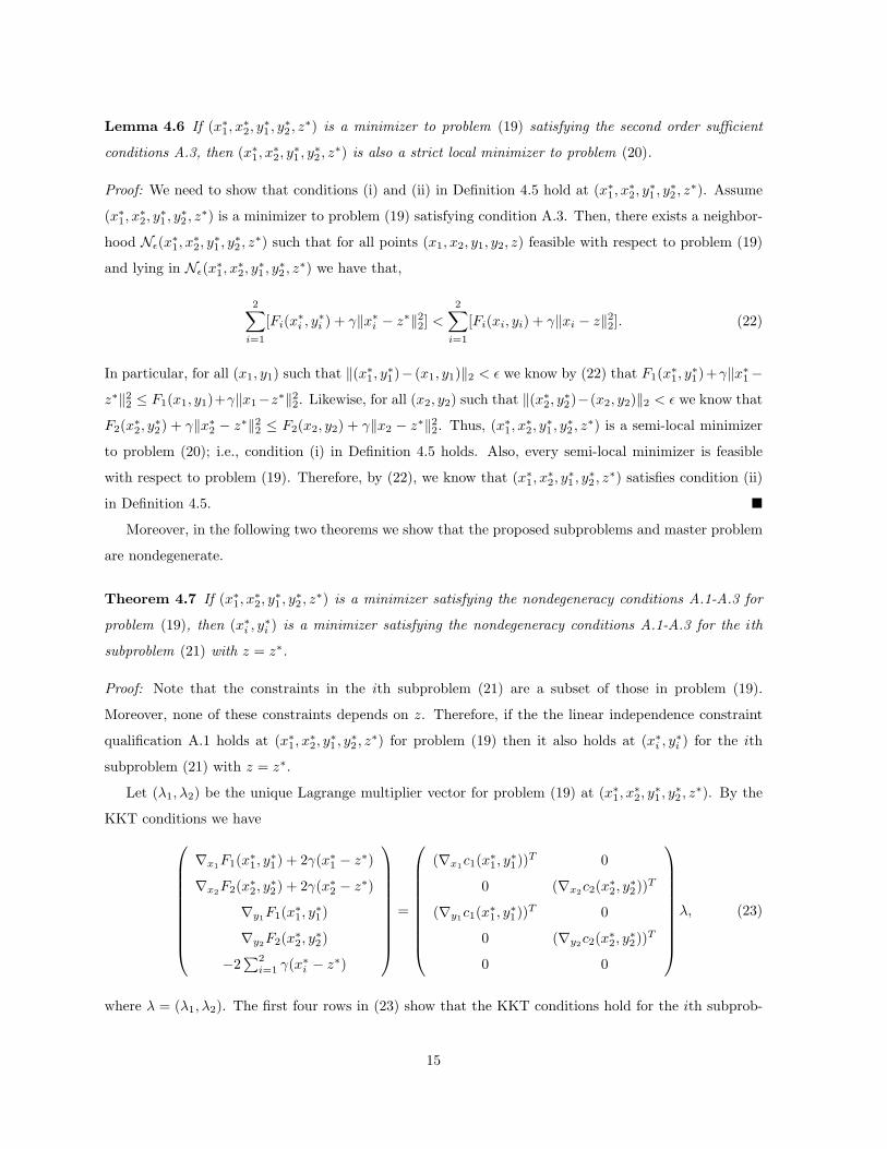
Theorem 5.1 Provided
γ >
∣
∣
∣
∣
∣
∣
∣
∣
∣
∣
∣
∣
∇xF1(x, y1) − (∇xc1(x, y1))Tλ1
∇xF2(x, y2) − (∇xc2(x, y2))Tλ2
∣
∣
∣
∣
∣
∣
∣
∣
∣
∣
∣
∣
∞
, (33)
a point (x, y1, y2) is a minimizer to problem (10) satisfying the nondegeneracy conditions A.1-A.3 with
Lagrange multipliers (λ1, λ2) if and only if the point (x1, x2, y1, y2, s1, s2, t1, t2, z) with s1, s2, t1, t2 = 0
and x1, x2, z = x is a minimizer to problem (32) satisfying the nondegeneracy conditions A.1-A.3 with
Lagrange multipliers
24
λ1
λ2
∇xF1(x, y1) − (∇xc1(x, y1))Tλ1
∇xF2(x, y2) − (∇xc2(x, y2))Tλ2
γe−∇xF1(x, y1) + (∇xc1(x, y1))Tλ1
γe−∇xF2(x, y2) + (∇xc2(x, y2))Tλ2
γe+ ∇xF1(x, y1) − (∇xc1(x, y1))Tλ1
γe+ ∇xF2(x, y2) − (∇xc2(x, y2))Tλ2
. (34)
Proof: First, we introduce some notation. Let
JT1 =
(∇xc1(x, y1))T (∇xc2(x, y2))
T
(∇y1c1(x, y1))
T
(∇y2c2(x, y2))
T
be the transposed Jacobian matrix for problem (10) and let JT1 be the submatrix of JT
1 composed only
by the gradients of those inequality constraints c1 and c2 that are active at (x, y1, y2). Likewise, let the
transposed Jacobian matrix for problem (32) be
JT2 =
(∇xc1(x, y1))T I
(∇xc2(x, y2))T I
(∇y1c1(x, y1))
T
(∇y2c2(x, y2))
T
I I
I I
−I I
−I I
−I −I
,
where I is the identity matrix of dimension n. Let JT2 be the submatrix of JT
2 composed only by the
gradients of the constraints active at the point (x1, x2, y1, y2, s1, s2, t1, t2, z) with s1, s2, t1, t2 = 0 and
x1, x2, z = x for problem (32).
Now we prove that the linear independence constraint qualification A.1 holds at (x, y1, y2) for problem
(10) iff it holds at (x1, x2, y1, y2, s1, s2, t1, t2, z) with s1, s2, t1, t2 = 0 and x1, x2, z = x for problem (32).
To see this, suppose that condition A.1 does not hold for problem (10). Thus, suppose there exists
(ψ1, ψ2) 6= 0 such that
JT1
ψ1
ψ2
= 0. (35)
Then it is easy to see that
JT2 ψ = 0, (36)
25

where ψ = (ψ1, ψ2, . . . , ψ8) with ψ3 = −ψ5 = ψ7 = −(∇xc1(x, y1))Tψ1, and ψ4 = −ψ6 = ψ8 =
−(∇xc2(x, y2))Tψ2. Thus, condition A.1 does not hold for problem (32). Conversely, it is easy to
show by similar arguments that if there exists ψ1, . . . , ψ8 6= 0 such that equation (36) holds, then (35)
holds for (ψ1, ψ2) 6= 0.
Now we turn to the KKT conditions. First, it is obvious that the feasibility conditions (47)–(48)
are satisfied at (x, y1, y2) for problem (10) iff they are satisfied at (x1, x2, y1, y2, s1, s2, t1, t2, z) with
s1, s2, t1, t2 = 0 and x1, x2, z = x for problem (32). Moreover, assume there exists (λ1, λ2) ≥ 0 satisfying
the complementarity condition (49) at (x, y1, y2) such that
∑2i=1 ∇xFi(x, yi)
∇y1F1(x, y1)
∇y2F2(x, y2)
= JT1
λ1
λ2
. (37)
Then we obviously have that
∇xF1(x, y1)
∇xF2(x, y2)
∇y1F1(x, y1)
∇y2F2(x, y2)
γe
γe
γe
γe
0
= JT2 λ, (38)
with λ as given by (34). Conversely, if there exists (λ1, λ2, . . . , λ8) satisfying equation (38), then
(λ1, λ2, . . . , λ8) must be as given in (34) and (37) is satisfied at (x, y1, y2) for problem (10) with (λ1, λ2).
Furthermore, it is clear that, provided condition (33) holds, the complementarity, nonnegativity, and
strict complementarity conditions [(49), (50), and A.2] hold at (x, y1, y2) for problem (10) with (λ1, λ2)
iff they hold at (x1, x2, y1, y2, s1, s2, t1, t2, z) with s1, s2, t1, t2 = 0 and x1, x2, z = x for problem (32) with
the Lagrange multiplier given by (34).
Finally, we turn to the second order sufficient conditions for optimality A.3. First, note that there
is a one-to-one correspondence between the vectors tangent to the inequality constraints active at
(x, y1, y2) for problem (10) and the vectors tangent to the equality and inequality constraints active at
(x1, x2, y1, y2, s1, s2, t1, t2, z) with with s1, s2, t1, t2 = 0 and x1, x2, z = x for problem (32). In particular,
given τ1 = (τx, τy1, τy2
) such that
J1τ1 = 0, (39)
we know that τ2 = (τx1, τx2
, τy1, τy2
, τs1, τs2
, τt1 , τt2 , τz) with τx1, τx2
, τz = τx and τs1, τs2
, τt1 , τt2 = 0
26

satisfies
J2τ2 = 0. (40)
Conversely, if τ2 satisfies (40), then we know that τx1, τx2
= τz, and that τs1, τs2
, τt1 , τt2 = 0 and
(τz, τy1, τy2
) satisfies (39). Finally, given τ1 and τ2 with τx1, τx2
, τz = τx and τs1, τs2
, τt1 , τt2 = 0, it
is easy to see from the form of problems (10) and (32) that τT1 ∇2L1 τ1 = τT
2 ∇2L2 τ2, where ∇2L1 is the
Hessian of the Lagrangian for problem (10) and ∇2L2 is the Hessian of the Lagrangian for problem (32).
�
The following theorem shows that for γ large enough, and assuming the gradients of the equality
constraints x1 = z, x2 = z, and the active inequalities c1(x1, y1) ≥ 0 and c2(x2, y2) ≥ 0 are linearly
independent, a local minimizer of problem (32) must be feasible with respect to problem (10).
Theorem 5.2 Assume there exists M such that X = (x1, x2, y1, y2, s1, s2, t1, t2, z) is a local minimizer
to problem (32) for all γ > M and such that the nondegeneracy conditions A.1-A.3 are satisfied at X
and the gradients of the equality constraints x1 = z, x2 = z, and the active inequalities c1(x1, y1) ≥ 0
and c2(x2, y2) ≥ 0 are linearly independent at X. Then, we must have that s1 = s2 = t1 = t2 = 0,
x1 = x2 = z, and the point (x, y1, y2) is a local minimizer to problem (10) satisfying the nondegeneracy
conditions A.1-A.3.
Proof: Assume there exists M such that for all γ > M , X is a nondegenerate minimizer of (32) at which
the gradients of the equality constraints x1 = z, x2 = z, and the active inequalities c1(x1, y1) ≥ 0 and
c2(x2, y2) ≥ 0 are linearly independent. Then, for any γ > M and ∆γ > 0, we must have that X is a
local minimizer of (32) for both γ and γ = γ + ∆γ. Therefore, the KKT conditions must hold for both
γ and γ at X. Subtracting these two sets of KKT conditions we get the following equation
0
0
0
0
∆γe
∆γe
∆γe
∆γe
0
= JT2 ∆λ, (41)
where J2 is the Jacobian matrix of the equality and active inequality constraints at X. The proof
continues by contradiction. Assume that some of the nonnegativity bounds si ≥ 0, ti ≥ 0 were not
active at X (that is, assume the gradients of some of the nonnegativity bounds were not in JT2 ). Then,
because the left-hand side of (41) is a linear combination of the gradients of the nonnegativity bounds
and J2 does not contain the gradients of all these nonnegativity bounds, we have that (41) would imply
27

that the gradients of the equality constraints xi + si − ti = z, the nonnegativity bounds si, ti ≥ 0 for
i = 1, 2, and the active inequalities ci(xi, yi) ≥ 0 for i = 1, 2 are linearly dependent. But note that this
contradicts the assumption that the gradients of the equality constraints x1 = z, x2 = z, and the active
inequalities c1(x1, y1) ≥ 0 and c2(x2, y2) ≥ 0 are linearly independent at X, because it is easy to see that
the gradients of the equality constraints x1 = z, x2 = z are linearly independent at X if and only if the
gradients of the equality constraints x1 + s1 − t1 = z, x2 + s2 − t2 = z, and the gradients of all (active
and inactive) nonnegativity bounds si ≥ 0, ti ≥ 0 are linearly independent. Thus, we must have that
s1 = s2 = t1 = t2 = 0 and thus x1 = x2 = z. Then, the result then follows from Theorem 5.1. �
5.3.3 Introducing barrier terms
The second transformation operated on problem (10) in order to obtain the desired master problem is the
introduction of barrier terms to remove the nonnegativity bounds. The result is the following problem:
minxi,yi,si,ti,z
2∑
i=1
[Fi(xi, yi) + γeT (si + ti) − µn∑
j=1
(log sij + log tij)]
s.t. ci(xi, yi) ≥ 0, i = 1, 2,
xi + si − ti = z, i = 1, 2,
(42)
where µ is the barrier parameter.
Barrier functions have been extensively analyzed in the nonlinear optimization literature. The follow-
ing two theorems establish the mathematical equivalence of problems (32) and (42). The first theorem
follows from Theorems 14 and 17 in [15] and shows that, given a nondegenerate minimizer of problem
(32), there exists a trajectory of nondegenerate minimizers to problem (42) that converge to it.
Theorem 5.3 If X = (x1, x2, y1, y2, s1, s2, t1, t2, z) is a minimizer satisfying the nondegeneracy condi-
tions A.1-A.3 for problem (32), then there exists ǫ > 0 such that for µ ∈ (0, ǫ) there exists a unique once
continuously differentiable trajectory of minimizers to problem (42) X(µ) satisfying the the nondegeneracy
conditions A.1-A.3 such that limµ→0X(µ) = X.
The second theorem follows from Theorem A.4 in the Appendix and shows that any accumulation
point of nondegenerate local minimizers to problem (42) is a KKT point of problem (32).
Theorem 5.4 Let {(x1, x2, y1, y2, s1, s2, t1, t2, z)}k be a sequence of KKT points for problem (42) at which
condition A.1 holds and corresponding to a sequence of positive barrier parameters {µ}k with limk→∞ µk =
0. Then, any limit point (x∗1, x∗
2, y∗
1 , y∗
2 , s∗
1, s∗
2, t∗
1, t∗
2, z∗) of the sequence {(x1, x2, y1, y2, s1, s2, t1, t2, z)}k
at which the gradients of the active constraints of problem (32) are linearly independent is a KKT point
of problem (32) at which condition A.1 holds.
28

5.3.4 Decomposition
We now consider the last transformation operated on the MDO problem. Note that problem (42) can be
decomposed into N independent subproblems by simply setting the target variables to a fixed value. The
subproblem optimal-value functions can then be used to define a master problem. The result is the EPD
master problem
minz
2∑
i=1
F ∗
i (z), (43)
where F ∗
i (z) is the ith subproblem optimal-value function,
minxi,yi,si,ti
Fi(xi, yi) + γeT (si + ti) − µ∑n
j=1(log sij + log tij)
s.t. ci(xi, yi) ≥ 0,
xi + si − ti = z.
(44)
In this section, we show that problems (42) and (43)-(44) are mathematically equivalent. The proof
to the following lemma parallels that of Lemma 4.6.
Lemma 5.5 If (x1, x2, y1, y2, s1, s2, t1, t2, z) is a minimizer to problem (42) satisfying the second order
sufficient conditions A.3, then it is also a strict local minimizer to problem (43).
In the following two theorems we show that the proposed subproblem and master problem are non-
degenerate.
Theorem 5.6 If (x1, x2, y1, y2, s1, s2, t1, t2, z) is a minimizer satisfying the nondegeneracy conditions
A.1-A.3 for problem (42), then (xi, yi, si, ti) is a minimizer satisfying the nondegeneracy conditions A.1-
A.3 for the ith subproblem (44) with z.
Proof: Note that, because of the elastic variables, the gradients of the equality constraints in the ith
subproblem (44) are always linearly independent from the gradients of the active inequality constraints.
Moreover, if the linear independence constraint qualification holds for problem (42) then the gradients of
the inequality constraints ci(xi, yi) active at (xi, yi, si, ti) must be linearly independent. Therefore, the
linear independence constraint qualification A.1 holds for the ith subproblem.
Now we turn to proving that the KKT conditions hold for the ith subproblem. Let (λ1, λ2, λ3, λ4)
be the unique Lagrange multiplier vector for problem (42) at (x1, x2, y1, y2, s1, s2, t1, t2, z). By the KKT
conditions we have
29

∇x1F1(x1, y1)
∇x2F2(x2, y2)
∇y1F1(x1, y1)
∇y2F2(x2, y2)
γe+ µS−11 e
γe+ µS−12 e
γe+ µT−11 e
γe+ µT−12 e
0
=
(∇x1c1(x
∗
1, y∗
1))T 0 I 0
0 (∇x2c2(x
∗
2, y∗
2))T 0 I
(∇y1c1(x
∗
1, y∗
1))T 0 0 0
0 (∇y2c2(x
∗
2, y∗
2))T 0 0
0 0 I 0
0 0 0 I
0 0 −I 0
0 0 0 −I
0 0 −I −I
λ, (45)
where Si and Ti are the diagonal matrices whose diagonal are the vectors si, ti, and λ = (λ1, λ2, λ3, λ4).
Notice that by the first, third, fifth, and seventh rows in (45) imply the KKT conditions hold for the
first subproblem. Likewise, the second, fourth, sixth, and eighth rows imply that the KKT conditions
hold for the second subproblem. Moreover, if the strict complementarity slackness conditions A.2 hold
for problem (42) with (λ1, λ2, λ3, λ4), then they obviously also hold for the first subproblem (44) with
(λ1, λ3) and for the second subproblem with (λ2, λ4).
It only remains to show that the second order sufficient conditions for optimality A.3 hold for the ith
subproblem (44). Let τ1 = (τx1, τy1
, τs1, τt1) be tangent to the equality and active inequality constraints
at (x1, y1, s1, t1) for the first subproblem (44). Then the vector τ2 = (τx1, τx2
, τy1, τy2
, τs1, τs2
, τt1 , τt2 , τz)
with τx2, τy2
, τs2, τt2 , τz = 0 is tangent to the equality and active inequality constraints for problem (42).
Moreover, it is easy to see that τT1 L1τ1 = τT
2 ∇2L2τ2, where ∇2L1 is the Hessian of the Lagrangian for the
first subproblem (44), and ∇2L2 is the Hessian of the Lagrangian for problem (42). The same argument
can be applied for the second subproblem. �
The proof to the following theorem parallels that of Theorem 4.8
Theorem 5.7 If Fi and ci are three times continuously-differentiable and the point (x1, x2, y1, y2, s1, s2, t1, t2, z)
is a minimizer to problem (42) satisfying the nondegeneracy conditions A.1-A.3, then:
1. the objective function of the master problem (43) can be defined locally as a twice continuously-
differentiable function F ∗(z) in a neighborhood Nǫ(z),
2. z is a minimizer to F ∗(z) satisfying the second order sufficient conditions.
Finally, the proof of the following Theorem parallels that of Theorem 4.11.
Theorem 5.8 Let (x1, x2, y1, y2, s1, s2, t1, t2, z) be a local minimizer of (43)-(44) satisfying conditions
A.1-A.3 for the subproblems (44), then (x1, x2, y1, y2, s1, s2, t1, t2, z) is a KKT point for problem (42) at
which condition A.1 holds.
30

5.3.5 Summary
The following two theorems summarize the mathematical equivalence and nondegeneracy results for EPD.
Note that the assumptions are equivalent to those made in the analysis of IPD.
Theorem 5.9 Let (x, y1, y2) be a minimizer to problem (10) satisfying the nondegeneracy conditions
A.1-A.3, then there exists M such that for γ > M and for µ sufficiently small, there exists a locally
unique once continuously-differentiable trajectory of local minimizers to problem (43)-(44) satisfying the
nondegeneracy conditions A.1-A.3 for the subproblems (44) and condition A.3 for problem (43) and such
that
limµ→0
(x1(µ), x2(µ), y1(µ), y2(µ), s1(µ), s2(µ), t1(µ), t2(µ), z(µ)) = (x, x, y1, y2, 0, 0, 0, 0, x).
Proof: The result follows from Theorems 5.1, 5.3, 5.5, 5.6, and 5.7, with the existence of a finite M is
guaranteed by Theorem 5.1. �
Theorem 5.10 Let {X}k = {(x1, x2, y1, y2, s1, s2, t1, t2, z)}k be a sequence of local minimizers of problem
(43)-(44) corresponding to a sequence of barrier parameters {µ}k with limk→∞ µk = 0 and such that the
nondegeneracy conditions A.1-A.3 are satisfied for the subproblems (44) at {X}k. Moreover, let X∗ be a
limit point of the sequence {X}k at which the gradients of the equality constraints x∗1 = z∗, x∗2 = z∗, and
the active inequality constraints c1(x∗
1, y∗
1) and c2(x∗
2, y∗
2) are linearly independent. Then, there exists M
such that if γ > M , X∗ is a KKT point of problem (10) at which condition A.1 holds.
Proof: The result follows from Theorems 5.1, 5.2, 5.4, and 5.8, with the existence of a finite M guaranteed
by Theorem 5.1. �
5.4 Local Convergence
In the following theorem we show that, for each value of the barrier parameter, the BFGS quasi-Newton
method proposed to solve the master problem (Step 2 in Figure 2) converges locally at a superlinear rate.
Moreover, we show that the primal-dual interior-point method PDSOL converges locally at a superlinear
rate when applied to the subproblem (44).
Theorem 5.11 Let (x∗, y∗1 , y∗
2) be a minimizer to problem (10) satisfying the nondegeneracy conditions
A.1-A.3. Then:
1. There exists a locally unique twice continuously-differentiable trajectory z∗(µ) of minimizers to
F ∗(z) defined for µ ∈ (0, ǫ1) for some ǫ1 > 0, such that limµ→0 z∗(µ) = x∗. Moreover, for each
µ ∈ (0, ǫ1) the minimizer z∗(µ) satisfies the second order sufficient conditions A.3.
31

2. For each µ ∈ (0, ǫ1), there exists ǫ2 > 0 such that if ‖z0−z∗(µ)‖ < ǫ2, then the iterates zk generated
by the BFGS quasi-Newton method (Step 2 in Figure 2) converge locally and superlinearly to z∗(µ).
3. For each µ ∈ (0, ǫ1), there exists ǫ2 > 0 such that there exists a locally unique trajectory
(xi(zk), yi(zk), si(zk), ti(sk)) of minimizers to the ith subproblem (44) satisfying the nondegeneracy
conditions A.1-A.3 defined for ‖zk − z∗(µ)‖ < ǫ2.
4. For each µ ∈ (0, ǫ1), there exists ǫ2 > 0 such that if ‖zk − z∗(µ)‖ < ǫ2, the iterates generated
by PDSOL converge locally and superlinearly to (xi(zk), yi(zk), si(zk), ti(sk)) when applied to the
subproblem (44) with z = zk.
Proof: Part 1 follows from Theorems 5.1, 5.3, and 5.7. To prove Part 2, note that from Theorem 5.7 we
know that F ∗(z) may be defined locally as a twice continuously-differentiable function and its Hessian
matrix is positive definite at z∗(µ). The local and superlinear convergence of the iterates generated by
the master problem algorithm follows from standard theory for quasi-Newton unconstrained optimization
algorithms [16].
From Theorems 5.1, 5.3, and 5.6 we know that there exists a minimizer to the ith subproblem
(44) (xi(z∗(µ)), yi(z
∗(µ)), si(z∗(µ)), ti(z
∗(µ))) for z = z∗(µ) satisfying the nondegeneracy conditions
A.1-A.3. Then, Part 3 follows from the nondegeneracy of (xi(z∗(µ)), yi(z
∗(µ)), si(z∗(µ)), ti(z
∗(µ))) and
the implicit function theorem [14]. Finally, the local and superlinear convergence of PDSOL (Part 4)
when applied to the subproblem (44) follows from the nondegeneracy of the ith subproblem minimizer
(xi(zk), yi(zk), si(zk), ti(zk)) given by Part 3 and standard convergence theory for primal-dual interior-
point methods [34]. �
6 Numerical Results
In the previous sections, we have proved that IPD and EPD converge locally at a superlinear rate for each
value of the penalty and barrier parameter. The question remains, however, whether the ill-conditioning
usually associated with large values of the penalty parameter or small values of the barrier parameter
will hinder the numerical performance of IPD and EPD.
To address this question, in this section we give a preliminary analysis the numerical performance of
IPD and EPD. A thorough computational test is out of the scope of this paper and will be done elsewhere.
Our preliminary results show that the numerical performance of our algorithms is not seriously impacted
by the ill-conditioning of the penalty and barrier functions.
We test the algorithms on the nonlinear test problem set of DeMiguel and Murray [10], which is a
modification of the bilevel programming test problems by Calamai and Vicente [6]. The nature of these
test problems is such that the user can choose the test-problem size, convexity, and the type of constraint
32

qualification satisfied at the minimizer. Moreover, all local and global minimizers of the test problems
are known a priori.
We compare our algorithms with the Progressive Hedging Algorithm (PHA) [25]. The PHA uses an
augmented Lagrangian function to break the MDO problem into a set of subproblems. We ran IPD,
EPD, and PHA on 30 test problems from [10]. For PHA, we use three different values of the penalty
parameter γ = 0.01, 1, 100. All results were obtained using MATLAB 5.3 on a Dell laptop with an 800
MHz Pentium III, 256MB RAM and running under WINDOWS 2000. The total time needed to solve
the 30 test problems was less than two hours.
The results are given in Table 1. The first four columns give information about the test problem.
The first column indicates whether the test problem is a quadratic program (Q) or a nonlinear program
(N). The second column indicates whether the test problem is convex (C) or nonconvex (N). The third
column indicates whether the test problem satisfies the linear independence constraint qualification (L)
or the strong linear independence constraint qualification (S); the strong linear independence constraint
qualification holds if for i = 1 : N the matrix ∇yici(x, yi) has full row rank. Finally, the fourth column
is the number of variables of the test problem.
The numerical performance of each decomposition algorithm is described by two columns. The first
column gives the number of subproblems that had to be solved in order to find the overall minimizer. This
quantity measures the amount of communication required between the master problem and the subprob-
lems. In situations were this communication is expensive, such as in the context of the multidisciplinary
design optimization problem, this is the main measure of the effectiveness of a decomposition algorithm.
We interrupted the execution of the decomposition algorithms when a maximum of 400 subproblems were
solved; that is, a 400 means the decomposition algorithm failed to find a stationary point after solving
400 subproblems. The second column is the average number of function evaluations needed to solve each
subproblem. Finally, note that IPD could not be applied to solve nonlinear test problems because the
subproblem solver PDSOL is capable of solving only quadratic programs.
The main insight from the numerical results is that whereas IPD and EPD found stationary points for
all test problems, PHA reached the maximum number of subproblems (400) without finding a stationary
point for most of the test problems and for all three values of the penalty parameter. The reason is that
while IPD and EPD converge at a superlinear rate for each value of the penalty and barrier parameters,
the PHA achieves only a linear convergence rate and, for the test problems tried, with a convergence
constant very close to one. Table 2 illustrates the typical convergence rate of the three algorithms.
Note that the number of subproblems that had to be solved in order to find the overall minimizer
is quite similar for IPD and EPD. However, the average number of function evaluations needed to solve
each subproblem is substantially larger for IPD. The reason for this is that the IPD subproblem solver
(NPSOL) makes use only of first derivatives, whereas the EPD subproblem solver (PDSOL) uses also
33

Test ProblemIPD EPD PHA
γ : 0.01PHA
γ : 1PHA
γ : 102
sub fun sub fun sub fun sub fun sub fun
Q C S 42 12 47 13 9 400 39 103 29 400 31Q C S 84 27 80 24 11 400 77 400 72 400 62Q C S 126 33 109 23 12 400 90 400 80 400 92Q C S 168 34 149 41 12 400 113 400 81 400 158Q C S 210 66 165 111 12 400 141 400 159 400 126Q C L 42 68 24 57 7 400 21 39 17 159 37Q C L 84 133 49 91 8 400 35 193 42 400 63Q C L 126 170 47 248 8 400 15 342 23 400 69Q C L 168 220 73 299 10 400 26 400 54 400 107Q C L 210 348 75 351 10 400 24 400 133 400 104Q N S 42 10 47 11 7 36 12 173 18 400 43Q N S 84 20 79 23 10 400 26 400 71 400 67Q N S 126 17 119 33 12 211 25 400 90 400 113Q N S 168 17 154 30 25 145 27 400 105 400 149Q N S 210 33 186 99 14 400 127 400 170 400 162Q N L 42 83 28 103 7 400 23 39 15 122 35Q N L 84 147 54 221 8 400 41 108 56 400 62Q N L 126 224 62 297 9 400 54 119 44 400 63Q N L 168 281 86 307 10 400 73 293 47 400 110Q N L 210 331 109 397 11 400 86 400 146 400 121N N S 42 9 52 - - 400 13 120 38 400 44N N S 84 18 89 - - 400 52 400 73 400 69N N S 126 17 134 - - 400 36 400 123 400 109N N S 168 16 174 - - 186 69 400 140 400 153N N S 210 28 210 - - 400 182 400 152 400 153N N L 42 142 31 - - 400 24 46 33 400 45N N L 84 285 58 - - 400 70 400 77 400 61N N L 126 272 84 - - 400 87 386 83 400 100N N L 168 279 120 - - 400 98 140 98 400 149N N L 210 356 141 - - 400 123 400 148 400 155
Table 1: Numerical results: the first four columns describe the test problem. In the first column,Q means quadratic program and N means nonlinear program. In the second column, C means convex,N means nonconvex. In the third column, S means strong linear independence constraint qualificationand L means linear independence constraint qualification. The fourth column is the number of variables.For each algorithm we give the number of subproblems solved (sub) and the average number of functionevaluations per subproblem (fun). We interrupt the execution of an algorithm when it reaches 400subproblems. EPD can not solve nonlinear programs because the subproblem solver PDSOL is a quadraticprogramming solver.
34

Table 2: Typical convergence rate for IPD, EPD, and PHA.
IPD EPD PHA
1.71e-002 3.93e-002 1.57e-0051.95e-003 1.74e-003 1.54e-0051.09e-004 3.29e-004 1.50e-0056.57e-006 4.54e-006 1.46e-005
second derivatives. Notice also that the computational effort required to solve test problems satisfying
only the linear independence constraint qualification (LICQ) is an order of magnitude larger than that
required to solve test problems satisfying the strong linear independence constraint qualification (SLICQ).
This confirms that the distinction between LICQ and SLICQ is also important in practice.
To analyze the effect that the number of global variables has on the computational effort, we solved a
number of test problems with the same number of global variables but with an increasing number of local
variables. The number of subproblems needed to find a stationary point remained roughly constant for
all test problems. This seems to imply that the computational effort will depend mostly on the number
of global variables.
Finally, IPD and EPD successfully solved the two sample test problems proposed in [3] on which CO
failed.
7 Conclusion
We propose two bilevel decomposition algorithms and analyze their properties. Firstly, we show that they
are mathematically equivalent to MDO under mild assumptions. Secondly, we show that under standard
nondegeneracy assumptions on the MDO minimizer, the proposed master problem and subproblems are
nondegenerate as well. As a consequence, we show that they converge locally at a superlinear rate for
each value of the penalty and barrier parameters. Our preliminary computational experiments show that
the performance of our algorithms is not seriously impacted by the ill-conditioning associated with the
penalty and barrier functions. In fact, our algorithms perform better on the test problems tried than the
progressive hedging algorithm [25]. We believe IPD and EPD will be especially efficient when applied to
problems having only a few global variables and a large number of local variables.
Acknowledgements. We thank the Associate Editors and three referees for their detailed comments and sugges-
35

tions. We are grateful to R.W. Cottle, M.P. Friedlander, M.A. Saunders, S. Scholtes for many helpful comments.
We would also like to acknowledge comments from seminar participants at Stanford University, London Business
School, Cambridge University, Universidad Carlos III de Madrid, INFORMS International Conference (Hawaii,
2001), Argonne National Laboratory, and Nortwestern University. Financial support for this research was pro-
vided by the La Caixa Fellowship Program, the National Science Foundation Grant CCR-9988205, the Department
of Naval Research Grant 00014-96-1-0274, and General Motors under the GM/Stanford Collaborative Research
Laboratory in Work Systems.
A Optimality Conditions
Consider a general nonlinear optimization problem of the form
minx
F (x)
s.t. c(x) ≥ 0,
d(x) = 0,
(46)
where x ∈ Rn, c : Rn → Rm, and d : Rn → Rp.
Definition A.1 The linear independence constraint qualification holds at a feasible point x if the gradi-
ents of all active inequality constraints (∇ci(x), all i such that ci(x) = 0) and the gradients of all equality
constraints (∇di(x), i = 1 : p) are linearly independent.
Theorem [KKT conditions] Provided F , c and d are differentiable at x∗ and the linear independence
constraint qualification holds at x∗, if x∗ is a local minimizer then there exist vectors λ∗ and ν∗ such that
c(x∗) ≥ 0, (47)
d(x∗) = 0, (48)
c(x∗)Tλ∗ = 0, (49)
λ∗ ≥ 0, (50)
∇L(x∗, λ∗, ν∗) = 0, (51)
where the Lagrangian function L(x, λ, ν)L(x, λ, ν) = F (x) − c(x)Tλ+ d(x)T ν.
The triple (x, λ, ν) is a KKT point if it satisfies conditions (47)–(51).
Definition A.2 The strict complementarity slackness conditions hold at a first-order KKT point (x∗, λ∗, ν∗)
if exactly one of λ∗i and ci(x∗) is zero for each i = 1 : m.
36

Theorem A.3 Second order sufficient conditions that a point x∗ be an isolated local minimizer when F ,
c and d are twice differentiable at x∗, are that there exist vectors λ∗ and ν∗ satisfying conditions (47)–(51)
and for every τ satisfying
τT∇ci(x∗) = 0, ∀i ∈ D ≡ {i : λ∗i > 0},
τT∇ci(x∗) ≥ 0, ∀i ∈ B −D,
τT∇di(x∗) = 0, ∀i = 1:p.
we have that τT∇2L(x∗, λ∗, ν∗)τ > 0.
Theorem A.4 Let {x}k be a sequence of KKT points of the barrier problem
minx
F (x) − µ log(c(x))
s.t. d(x) = 0,(52)
corresponding to a sequence of positive barrier parameters {µ}k such that limk→∞ µk = 0. Then, any limit
point of {x}k at which the gradients of the equality constraints d(x) and the active inequality constraints
c(x) are linearly independent is a KKT point of problem (46).
Proof: Because {x}k is a sequence of KKT points of problem (52), we must have that for all k there exist
νk such that
∇F (xk) − (∇c(xk))TµkC(xk)−1e+ (∇d(xk))T νk = 0, (53)
where C(xk) is the diagonal matrix whose main diagonal is c(xk) and e is the vector of ones. Let x be a
limit point of {x}k. By taking limits as k → ∞ we obtain
∇F (x) − (∇c(x))T limk→∞
µkC(xk)−1e+ (∇d(x))T limk→∞
νk = 0. (54)
Note that for the inactive inequality constraints (ci(x) such that ci(x∗) > 0), we have that limk→∞ µk/ci(xk) =
0 because limk→∞ µk = 0 and ci(x∗) > 0. This together with (54) imply that
∇F (x) − (∇c(x))T limk→∞
µkC(xk)−1e+ (∇d(x))T limk→∞
νk = 0, (55)
where C(x) is the diagonal matrix whose main diagonal is the vector of active inequality constraints c(x).
Moreover, the linear independence of the gradients of c(x) and d(x) at the limit point x implies that there
exist unique and finite λ and ν such that λ = limk→∞ µkC(xk)−1e and ν = limk→∞ νk. Consequently,
condition (51) holds at x for problem (46) with the multipliers of the inactive inequality constraints equal
to zero, the multipliers of c(x) equal to λ, and the multipliers of d(x) equal to ν.
37

Also, note that if {x}k is a sequence of KKT points of (52), then limk→∞ d(xk) = d(x) = 0. Moreover,
because µk > 0 and, by the properties of the barrier function, c(xk) > 0, we must have that λ =
limk→∞ µkC(xk)−1e ≥ 0. Finally, by the definition of λ and the fact that limk→∞ µk = 0, we know that
the complementarity condition (49) must hold. �
References
[1] N.M. Alexandrov and M.Y. Hussaini (eds.), Multidisciplinary optimization: State of the art, Philadel-
phia, SIAM, 1997.
[2] N.M. Alexandrov and R.M. Lewis, Comparative properties of collaborative optimization and other
approaches to MDO, Proc., First ASMO UK/ISSMO conference on Engineering Design Optimization,
MCB Press, Jul 1999.
[3] , Analytical and computational aspects of collaborative optimization, Tech. Report TM-2000-
210104, NASA, 2000.
[4] R.D. Braun, Collaborative optimization: An architecture for large-scale distributed design., Ph.D.
thesis, Stanford University, 1996.
[5] R.D. Braun and I.M. Kroo, Development and application of the collaborative optimization architecture
in a multidisciplinary design environment, Multidisciplinary Design Optimization: State of the Art
(N.M. Alexandrov and M.Y. Hussaini, eds.), 1997.
[6] P.H. Calamai and L.N. Vicente, Generating quadratic bilevel programming test problems, ACM Trans-
actions on Mathematical Software 20 (1994), no. 1, 103–119.
[7] E.J. Cramer, J.E. Dennis, P.D. Frank, R.M. Lewis, and G.R. Shubin, Problem formulation for
multidisciplinary optimization, SIAM J. Optimization 4 (1994), no. 4, 754–776.
[8] A.V. DeMiguel, Two decomposition algorithms for nonconvex optimization problems with global vari-
ables, Ph.D. thesis, Stanford University, 2001.
[9] A.V. DeMiguel and W. Murray, An analysis of collaborative optimization methods, Eight
AIAA/USAF/NASA/ISSMO Symposium on Multidisciplinary Analysis and Optimization, 2000,
AIAA Paper 00-4720.
[10] , Generating optimization problems with global variables, Tech. Report SOL 01-3, Dept. of
Management Science and Engineering, Stanford University, 2001.
38

[11] , Two decomposition algorithms for nonconvex optimization problems with global variables,
Tech. Report SOL 01-1, Dept. of Management Science and Engineering, Stanford University, 2001.
[12] A.V. DeMiguel and F.J. Nogales, A superlinearly convergent interior-point decomposition algorithm
using low-cost subproblem solutions, Working paper, London Business School, 2002.
[13] S. Dempe, Foundations of bilevel programming, Kluwer Academic Publishers, Boston, 2002.
[14] A.V. Fiacco, Introduction to sensitivity and stability analysis in nonlinear programming, Academic
Press, New York, 1983.
[15] A.V. Fiacco and G.P. McCormick, Nonlinear programming: Sequential unconstrained minimization
techniques, John Wiley & Sons, New York, 1968.
[16] R. Fletcher, Practical methods of optimization, Wiley, New York, 1987.
[17] P.E. Gill, W. Murray, M.A. Saunders, and M.H. Wright, User’s guide for NPSOL (version 4.0),
Tech. Report SOL 86-2, Dept. of Operations Research, Stanford University, 1986.
[18] P.E. Gill, W. Murray, and M.H. Wright, Practical optimization, Academic Press, New York, 1981.
[19] R.T. Haftka and J. Sobieszczanski-Sobieski, Multidisciplinary aerospace design optimization: Survey
of recent developments, Structural Optimization 14 (1997), 1–23.
[20] R.T. Haftka and L.T. Watson, Multidisciplinary design optimization with quasiseparable subsystems,
Tech. Report TR-02-09, Computer Science, Virginia Polytechnic Institute and State University, 2002.
[21] Z.-Q. Luo, J.-S. Pang, and D. Ralph, Mathematical programs with equilibrium constraints, Cambridge
University Press, Cambridge, 1996.
[22] V.M. Manning, Large-scale design of supersonic aircraft via collaborative optimization., Ph.D. thesis,
Stanford University, 2000.
[23] W. Murray and F.J. Prieto, A sequential quadratic programming algorithm using an incomplete
solution of the subproblem, SIAM J. Optimization 5 (1995), no. 3, 590–640.
[24] J. Nocedal and S.J. Wright, Numerical optimization, Springer-Verlag, New York, 1999.
[25] R.T. Rockafellar and R.J-B. Wets, Scenarios and policy aggregation in optimization under uncer-
tainty, Mathematics of Operations Research 16 (1991), 119–147.
[26] J.F. Rodriguez, J.E. Renaud, and L.T. Watson, Convergence of trust region augmented lagrangian
methods using variable fidelity approximation data, Structural Optim. 15 (1998), 141–156.
39

[27] , Trust region augmented lagrangian methods for sequential response surface approximation
and optimization, ASME M. Mech. Design 120 (1998), 58–66.
[28] J. Shankar, C.J. Ribbens, R.T. Haftka, and L.T. Watson, Computational study of a nonhierarchical
decomposition algorithm, Comput. Optim. Appl. 2 (1993), 273–293.
[29] K. Shimizu, Y. Ishizuka, and J.F. Bard, Nondifferentiable and two-level mathematical programming,
Kluwer Academic Publishers, Boston, 1997.
[30] I.P. Sobieski, Multidisciplinary design using collaborative optimization., Ph.D. thesis, Stanford Uni-
versity, 1998.
[31] J. Sobieszczanski-Sobieski, Optimization by decomposition: a step from hierarchic to nonhierarchic
systems, Second NASA/Air Force Symp. on Recent Advances in Multidisciplinary Analysis and
Optimization, 1988.
[32] K. Tammer, The application of parametric optimization and imbedding for the foundation and real-
ization of a generalized primal decomposition approach, Parametric Optimization and Related Top-
ics (J. Guddat, H. Jongen, B. Kummer, and F. Nozicka, eds.), Mathematical Research, vol. 35,
Akademie-Verlag, Berlin, 1987.
[33] S.J. Wright, Primal-Dual Interior-Point Methods, SIAM, Philadelphia, 1997.
[34] H. Yamashita and H. Yabe, Superlinear and quadratic convergence of some primal–dual interior
point methods for constrained optimization, Mathematical Programming 75 (1996), :377–397.
40
![Convergence analysis of domain decomposition based … · Convergence analysis of domain decomposition based time integrators for degenerate parabolic equations ... [9, Chapter 1]](https://img.dokumen.tips/doc/110x75/5b30b9aa7f8b9ae16e8e78ce/convergence-analysis-of-domain-decomposition-based-convergence-analysis-of-domain.jpg)

![Deep Bilevel Learning - openaccess.thecvf.comopenaccess.thecvf.com/content_ECCV_2018/papers/Simon_Jenni_… · Deep Bilevel Learning Simon Jenni[0000−0002−9472−0425] and Paolo](https://img.dokumen.tips/doc/110x75/607b5cfda6b7d57d103f56ca/deep-bilevel-learning-deep-bilevel-learning-simon-jenni0000a0002a9472a0425.jpg)