A lexically scoped distributedpi-calculus

Antonio RavaraAna G. Matos

Vasco T. VasconcelosLuıs Lopes

DI–FCUL TR–02–4

April 2002

Departamento de InformaticaFaculdade de Ciencias da Universidade de Lisboa

Campo Grande, 1749–016 LisboaPortugal

Technical reports are available at http://www.di.fc.ul.pt/tech-reports. Thefiles are stored in PDF, with the report number as filename. Alternatively, reportsare available by post from the above address.

A lexically scoped distributed pi-calculus

Antonio Ravara∗ Ana G. Matos† Vasco T. Vasconcelos‡ Luıs Lopes†

April 2002

Abstract

We define the syntax, the operational semantics, and a type system for lsdπ,an asynchronous and distributed π-calculus with local communication and processmigration. The calculus follows a simple model of distribution for mobile calculi,with a lexical scoping mechanism that provides both for remote communication andfor process migration, making explicit migration primitives superfluous.

1 Introduction

Current hardware developments in network technology, namely high-bandwidth, low-laten-cy networks and wireless communication, has opened new prospects for mobile computa-tion, while at the same time introducing new problems that need to be addressed at thesoftware level. The fundamental problem stems from the lack of a formal background onwhich to assert the correctness of a given system specification. Thus, adequate theoreticalmodeling of distributed mobile systems is required to produce provably correct softwarespecifications and to reason about distributed computations.

We propose a natural framework to specify such systems, based on the π-calculus [10,11], with explicit distribution and process migration. Technically, the paper describes anasynchronous and distributed π-calculus, where each free channel belongs to a specificsite, fixed throughout the computation, further developing the work in reference [14]. Weadhere to the lexical scoping in a distributed context of Obliq [5], meaning that, in orderto determine where an a certain free channel belongs to, we just have to inspect the codefor the process where the channel occurs. The rule is simple: located channels a@s belongto the site where they are (explicitly) located, s; simple channels a are (implicitly) locatedat the current site, the site where the process they occur at is located.

To motivate the importance of lexical scoping in programming languages in general,consider the following function written in (a variant of) Pascal.

∗Department of Mathematics, Instituto Superior Tecnico. Lisbon, Portugal.†Department of Computer Science, Faculty of Sciences, University of Porto, Portugal.‡Department of Informatics, Faculty of Sciences, University of Lisbon, Portugal.

1

function f (): Integer;var x: Integer := 1;function g () : Integer;

begin g := x end;begin f := x + g () end;

A programmer writes the body of function g knowing that x is global to g, and developsfunction f keeping in mind that x is local to f, and that the x of g and that of f denote thesame variable. This is the kind of reasoning that programmers have been doing for decades,both in imperative (Algol, Pascal) and in functional (ML, Haskell) languages. It is intuitive,and accumulated experience has shown the concept to be right. Also, an unoptimizingcompiler assigns to variable x a memory, together with the remaining information relevantfor function f. In order to evaluate the expressions in the body of each function, the codegenerated must read the value of x: in f it performs a local operation (reading from thedata for the current activation), for g it first finds where the f’s activation is. The goodnews is that we do not need to abandon these ideas, when moving into distributed (andcode migrating) computing.

Consider a network where we declare a channel x within some site f, ask for the processx?()P to migrate to another site g, and, in parallel launch a receptor x?()Q located at x.Here is the network (in receptive distributed π [2]), and the one obtained after one reductionstep.

f [new x new x@fgo g. x?()P | g [x?()P] ‖x?()Q] f [x?()Q]

From the preceding discussion, the pertinent questions are: “where does channel x belongto?”, and “where is x to be stored?”. Analyzing the new x@f part, it would seem thatchannel x belongs to site f, but looking at the subnetworks for g and for f we cannot reallyconclude that. More importantly, we have no clue on where to place the queue for x, for wehave receptors for x at both sites g and f. Amadio et al. [2] filter out the above networks, byimposing a unique receiver property (as in π1 [1]), together with other restrictions (localityand receptiveness). Although this is done using a simple type system, it is an extra elementthat looks to us counter-intuitive and heavy.We address the above questions by imposing a lexical scope discipline to networks. In lsdπ,the above left network would reduce to:

new x@fg [x@f?()P’] ‖f [x?()Q]

where it is clear (in each of the three lines) that channel x belongs to site f, and thatthe queue for x should be at f. Process P’ (obtained from P by the application of anappropriate substitution) reflects the fact that P has migrated from f to g: free simplechannels (implicitly located at f) become attached to their site (channel y becomes y@f);free channels located at the target site g (say z@g) become simple (by dropping the @gpart), reflecting their new local status, ready for communication; all the remaining channelsremain unchanged. In lsdπ, programmers may refer to a channel a belonging to a site s

2

by its local name a or by its remote name a@s, reflecting two distinct views of a channel:the local view and the network (global) view. Allowing the two views greatly simplifiesthe programming task and allows a standard definition for reduction when combined withmigration. From an implementation point of view, this explicit notation provides a compilerwith precious information to generate code to access channels.

Explicitly located input/output processes (receptors x@f?(y)P and messages x@f!〈v〉,absent in every proposal to date) obviate the need for the go primitive, written spawn(s,P)in [1], go s.P in [2], or s::P in [8]. It suffices to attach to such processes the behavior of “mi-grating toward the site where they belong”: a message targeted at x@f must first migrateto f (thus becoming targeted at x) prior to engaging in some communication; a receptorwaiting on x@f must first migrate to f (thus waiting now on x) prior to engaging in anycommunication. In lsdπ, reduction is local, avoiding remote communication between sitesin such a ubiquitous operation. This pattern of interaction between clients and servers isan alternative paradigm of growing interest in programming distributed-systems. Clientsdo not interact remotely with a server. Rather, they move to the site of the server andinteract locally until the session ends. Then, they return to their site of origin. Local com-munication minimizes network traffic and improves scalability. Migration and reductionare intimately related. An input/output process either reduces locally or migrates over thenetwork depending on the prefix. This is highly convenient from an implementation pointof view since possible migration operations are clearly marked in the program. Moreover,since the migration units are either input or output processes, their implementation is fareasier than it would be for a generic process.

Lexical scope together with compound names introduce subtleties in the definition offree names. Consider the network r[(ν a) a@s!〈〉]. It is not clear whether channel a belongsto r or to s, as it is not obvious whether a@s should be free or bound. Now considerthe network r[b?(x)x?()(ν a) a@s!〈〉] interacting with another network r[b!〈c@t〉], yieldingt[c?()(ν a) a@s!〈〉]. We see that a belongs to whatever site x belongs to, possibly neither rnor s (t in this case). We address this problem by imposing syntactic restrictions onprocesses otherwise defined by a context-free grammar (rejecting, among others, the aboveprocesses), and we make sure that these restrictions carry through, all the way from alpha-congruence to reduction.

Our values are simple channels a and located channels a@s; parameters are simplechannels only. This means that we cannot rely on the usual substitution of the π-calculus,where one substitutes channels by channels. To make sure we got the concept right, westart with a general notion of substitution: a total function on names (sites, channels,located channels), defined along the lines of the substitution for the λ-calculus, by Hindleyand Seldin [9]. This function is then used to define name replacement (used in alpha-congruence), name instantiation (the substitution that arises from communication, as ina!〈v〉 | a?(x)P ), and name translation (the substitution that happens during migration, asin a@s!〈v〉 or a@s?(x)P ).

For the type system, we take a simplified form of that of Amadio et al. [2], which weadapt to deal with the lexical scope of channels. Types for channels are the usual typesin the simply typed π-calculus, Ch(γ1, . . . , γn), describing a channel capable of carrying a

3

series of channels of types γ1, . . . , γn [13]. For sites, we only capture the types of the (free)channels at the site: if a1 to an of types γ1 to γn contain the free channels of site s, thenwe assign to site s the type {a1:γ1, . . . , an:γn}. The type system is simple and intuitive—astraightforward extension of that for simply typed π-calculus [13]; it assumes types forsites only (types for channels are taken from that of the site the channel belongs to), andenjoys subject-reduction.

Distinctive features of lsdπ include: separate syntactic categories for processes and net-works (in the line of Dπ [8], but unlike dπr

1 [2], nomadic-pict [12], the join-calculus [7], andmobile ambients [6]), a syntactically flat structure of the network and local communication(like Dπ, dπr

1, but unlike the join-calculus and ambients).Specifically, the contributions of this work are:

1. a distributed π-calculus that provides for local communication, remote invocation,weak mobility in a lexical scope regime;

2. a rigorous treatment of channels, allowing for the substitution of a channel by acompound channel, ensuring that each channel belongs to a unique, lexically defined,site;

3. a type system revealing the site of each channel, while ensuring subject-reduction.

The rest of the report is organized as follows: the next section presents the syntaxof the calculus; the operational semantics is dealt in section 3; section 4 describes typesand type assignment; and section 5 compares lsdπ with related work and points to futuredevelopments. Detailed proofs for all the results can be found in the appendix.

2 The calculus

This section presents the (context-free) grammar of the calculus, followed by the syntacticrestrictions.

2.1 Syntax

Consider a countable set C of simple channels a, b, c, x, y, z, and a countable set S ofsites s, r, t, such that the two sets are disjoint. Compound channels—pairs channel-site,like a@s—form located channels, designating a channel a at site s, belonging to the set

C@S def= {a@s | a ∈ C ∧ s ∈ S}. Let u, v, . . . stand for both simple and located channels,

henceforth collectively called channels. Take x as a variable ranging over simple channels,x as a sequence of pairwise distinct variables, let |x| denote the length of the sequence x,and let {x} denote the set of the channels in the sequence x; moreover, let v stand for asequence of channels. Furthermore, let n, m stand for both sites and channels, henceforth

collectively called names, and belonging to the set N def= C ∪S ∪C@S. Finally, let g, h stand

for both sites and located channels, henceforth collectively called global names.

4

Simple channels, a, b, c, x, y, z ∈ CSites, r, s, t ∈ S

Channels, u, v ::= a | a@s

Globals, g, h ::= a@s | s

Names, n, m ::= a | a@s | s

Processes, P, Q ::= 0 | (P |Q) | (ν n) P | u!〈v〉 | u?(x)P

Networks, N, M ::= 0 | (N ‖M) | (ν g) N | s[P ]

Figure 1: Syntax.

Definition 2.1 (Names, processes and networks). The grammars in figure 1 definethe languages of processes and of networks.

Receptors, of the form u?(x)P , and messages, of the form u!〈v〉, are the basic processesin the calculus. A receptor is an input-guarded process. A message has a name u fortarget and carries a sequence of channels v (note that we do not allow to pass sites). Theremaining constructors are fairly standard in name-passing process calculi: process (P |Q)denotes the parallel composition of processes; process (ν n) P denotes the restriction of thescope of the name n to the process P (often seen as the creation of a new name or site,visible only within P ; moreover, if n∈S, no channel explicitly located at that site is visibleoutside P ); and inaction 0, denotes the terminated process. For the sake of simplicity, werestrict this work to finite processes.

Networks are: processes running at a given site, s[P ], where we assume that free simplechannels in P are implicitly located at s (while located channels are considered to beexplicitly located); the parallel composition of networks, (N ‖M), which is simply a mergeof networks; the restriction of the scope of a global to a network, (ν g) N; and inaction 0,which denotes the empty network.

As usual in polyadic mobile calculi, we abbreviate (ν n1) · · · (ν nm) P to (ν n) P . Letthe operator ‘ν’ extend as far to the right as possible. In (P |Q), we omit the parentheseswhen the meaning is clear.

2.2 Free and bound names

We envisage a “natural” definition for the free names of a process or of a network, accordingto the classical definitions for the λ-calculus [3, 9], and meeting the intuitions of any π-calculist.

Notation 2.2 (Useful sets). Let A, B ⊆N .

5

N fn(N) bn(N)0 {} {}(N ‖M) fn(N) ∪ fn(M) bn(N) ∪ bn(M)(ν s) N fn(N) \ ({s} ∪ fn(N)@s) bn(N) ∪ {s} ∪ bn(N)@s(ν a@s) N fn(N) \ {a@s} ∪ {s} bn(N) ∪ {a@s}s[P ] locate(fn(P ), s) ∪ {s} locate(bn(P ), s)

Figure 2: Free and bound names in networks.

P fn(P ) bn(P )0 {} {}(P |Q) fn(P ) ∪ fn(Q) bn(P ) ∪ bn(Q)(ν s) P fn(P ) \ ({s} ∪ fn(P )@s) bn(P ) ∪ {s} ∪ bn(P )@s(ν a@s) P fn(P ) \ {a@s} ∪ {s} bn(P ) ∪ {a@s}(ν a) P fn(P ) \ {a} bn(P ) ∪ {a}u!〈v〉 names(u, v) {}u?(x)P fn(P ) \ {x} ∪ names(u) bn(P ) ∪ {x}

Figure 3: Free and bound names in processes.

1. A@sdef= {a@s | a ∈ A ∨ a@s ∈ A};

2. a@Bdef= {a@s | s ∈B};

3. names(n1 . . . nm)def= names(n1) ∪ . . . ∪ names(nm),

where names(s)def= {s}, names(a@s)

def= {a@s, s}, and names(a)

def= {a};

4. locate(A, s)def= A \ C ∪ A@s;

5. sites(A)def= {s | s ∈ A ∨ a@s ∈ A}.

Moreover, we say that s ∈ n when n ∈ C@s ∪ {s}, and a ∈ n when n ∈ a@S ∪ {a}.

Definition 2.3 (Free and bound names). The rules in Figures 2 and 3 inductivelydefine the sets of free and bound names in networks, fn(N) and bn(N), and in processes,fn(P ) and bn(P ).

A channel is local to a site if it occurs as a simple channel in that site, or if it occursexplicitly located at that site anywhere in the network. Amongst the binders of the calculus,two cases deserve a special mention: (ν s) N makes all free channels local to s invisibleoutside N ; and (ν a@s) N creates a new free site s. The free names of a network s[P ]are the free names of P where the simple channels are made explicitly located at s, viaoperator locate.

6

2.3 Syntactic restrictions

In lsdπ it is crucial to distinguish local from remote channels. However, the binders maycause undesirable side effects, leading to confusions like those described in the introduction.Therefore, we do not accept all terms resulting from the grammar in Definition 2.1 asprocesses: we impose syntactic restrictions. To rigorously define them, we use the auxiliarynotions of subnetworks and of subprocesses, which result from Definition 2.1.

Remark 2.4 (Subnetworks and subprocesses). One easily defines the set SN (N) ofthe subnetworks of the network N , and the set SP(P ) of the subprocesses of the process P .

We impose two conditions to accept a term as a process:

1. when a located channel has its scope restricted to some process, it cannot be used inthat process as a simple channel; and

2. similarly, when a simple channel has its scope restricted to some process, it can notbe used in that process as a located channel.

Since these are syntactic conditions, relying on the notions of free and bound names,one can easily state (decidable) properties that capture them. The following definitionrigorously states what terms we accept as processes.

Definition 2.5 (Syntactic restrictions).

1. A process P satisfies the syntactic restrictions, and we write P ok, if for all Q∈SP(P ),we have Q ok, and:

(a) if Q = (ν a@s) R, then a 6∈ fn(R); and

(b) if Q = (ν a) R, then a@S ∩ fn(R) = ∅; and

(c) if Q = u?(x)R, then⋃

x∈{x} x@S ∩ fn(Q) = ∅.

2. A network N satisfies the syntactic restrictions, and we write N ok, if all its subnet-works and all its subprocesses are ok.

In order to understand the need for these syntactic restrictions we have to take intoconsideration the fundamental ideas of lsdπ. As in [14], we embody a rule taken fromHennessy and Riely [8] which considers the network (ν a@s) s[P ] as indistinguishable fromthe network s[(ν a) P ] (forthcoming structural congruence rule SN-SCOS3). Also, we fixthat fn((ν a@s) N)= fn(N)\{a@s}, because we want the binder to capture only the channela local to site s (and this is a distinctive feature from Dπ, where all free occurrences of ain N are bound). If a process of the form (ν a) P , where a@s ∈ fn(P ), was to be accepted,one would have to decide whether a@s is free in such a process.

Therefore, to define the free variables of networks and processes, one should considerthree reasonable possibilities:

7

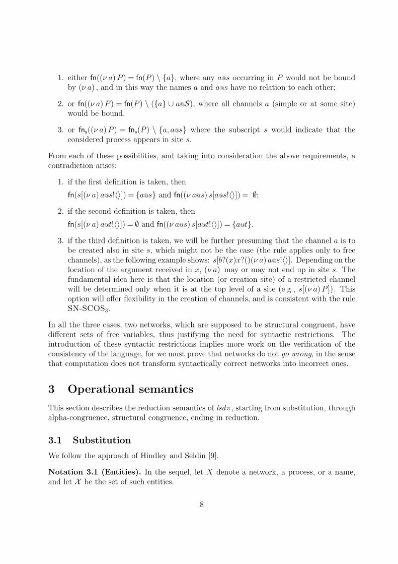
1. either fn((ν a) P ) = fn(P ) \ {a}, where any a@s occurring in P would not be boundby (ν a) , and in this way the names a and a@s have no relation to each other;

2. or fn((ν a) P ) = fn(P ) \ ({a} ∪ a@S), where all channels a (simple or at some site)would be bound.

3. or fns((ν a) P ) = fns(P ) \ {a, a@s} where the subscript s would indicate that theconsidered process appears in site s.

From each of these possibilities, and taking into consideration the above requirements, acontradiction arises:

1. if the first definition is taken, then

fn(s[(ν a) a@s!〈〉]) = {a@s} and fn((ν a@s) s[a@s!〈〉]) = ∅;

2. if the second definition is taken, then

fn(s[(ν a) a@t!〈〉]) = ∅ and fn((ν a@s) s[a@t!〈〉]) = {a@t}.

3. if the third definition is taken, we will be further presuming that the channel a is tobe created also in site s, which might not be the case (the rule applies only to freechannels), as the following example shows: s[b?(x)x?()(ν a) a@s!〈〉]. Depending on thelocation of the argument received in x, (ν a) may or may not end up in site s. Thefundamental idea here is that the location (or creation site) of a restricted channelwill be determined only when it is at the top level of a site (e.g., s[(ν a) P ]). Thisoption will offer flexibility in the creation of channels, and is consistent with the ruleSN-SCOS3.

In all the three cases, two networks, which are supposed to be structural congruent, havedifferent sets of free variables, thus justifying the need for syntactic restrictions. Theintroduction of these syntactic restrictions implies more work on the verification of theconsistency of the language, for we must prove that networks do not go wrong, in the sensethat computation does not transform syntactically correct networks into incorrect ones.

3 Operational semantics

This section describes the reduction semantics of lsdπ, starting from substitution, throughalpha-congruence, structural congruence, ending in reduction.

3.1 Substitution

We follow the approach of Hindley and Seldin [9].

Notation 3.1 (Entities). In the sequel, let X denote a network, a process, or a name,and let X be the set of such entities.

8

0[ ]def= 0

(N ‖M)[n/m]def= N [n/m] ‖M [n/m]

((ν s) N)[n/m]def= (ν s) N if s ∈ m

((ν s) N)[n/m]def= (ν s) N [n/m] if s /∈ m and (1)

((ν s) N)[n/m]def= (ν t) N [t/s][n/m] if s /∈ m and ¬(1), with t fresh

((ν a@s) N)[n/a@s]def= (ν a@s) N

((ν a@s) N)[n/s]def= (ν a@n) N [n/s]

((ν a@s) N)[n/m]def= (ν a@s) N [n/m] if m /∈ {s, a@s} and (2)

((ν a@s) N)[n/m]def= (ν b@s) N [b@s/a@s][n/m] if m /∈ {s, a@s} and ¬(2), with b fresh

(s[P ])[b@s/a@s]def= s[P [b/a][b@s/a@s]]

(s[P ])[n/s]def= n[P [n/s]]

(s[P ])[n/m]def= s[P [n/m]] if s /∈ m

(1) s /∈ n or m /∈ fn(N) ; (2) n /∈ {a, a@s} or m /∈ fn(N).

Figure 4: Substitution on networks.

Definition 3.2 (Substitution). A substitution on names in an entity is a total functionX [N /N ] 7→ X , inductively defined by the rules in the Figures 4, 5, and 6.

The substitution function gives rise to three different operations on names: change ofbound names ; communication; and migration. The first will be used to define the alpha-congruence relation and the others to define the reduction relation. To avoid confusion,the application of the substitution function in each of these operations will be referred toas, respectively, name replacement, name instantiation and name translation.

Definition 3.3 (Name replacement/instantiation/translation). Take the finite se-quence of substitutions [n1/m1] · · · [nk/mk]. Then, ∀i ∈ {1, . . . , k}, this sequence is a:

1. name replacement, if mi ∈ A ⇒ ni ∈ A, for A = C,S, C@s, for some s.

2. name instantiation, if mi ∈ C and ni ∈ C ∪ C@S.

3. name translation, if mi = a ⇒ ni ∈ a@S or mi ∈ a@S ⇒ ni = a.

Substitution presents two properties, which follow from the reasonable requirement ofthe names involved in such operations being of the “same nature”, as defined above: itcommutes with the free names and preserves the syntactic restrictions. In order to establishthe first result, it is usefull to extend the notion of substitution.

9

0[ ]def= as in the Networks case

(P |Q)[n/m]def= as in the Networks case

((ν s) P )[n/m]def= as in the Networks case

((ν a@s) P )[n/m]def= as in the Networks case

((ν a) P )[n/a]def= (ν a) P

((ν a) P )[n/m]def= (ν a) P [n/m] if (1) and (2)

((ν a) P )[n/m]def= (ν b) P [b/a][n/m] if (1) and ¬(2), with b fresh

(u!〈v1 . . . vn〉)[n/m]def= u[n/m]!〈v1[n/m] . . . vn[n/m]〉

(u?(x)P )[n/xi]def= u[n/xi]?(x)P if xi ∈ {x}

(u?(x)P )[n/m]def= u[n/m]?(x)P [n/m] if (3) and (4)

(u?(x)P )[n/m]def= u[n/m]?(x1..y..xn)P [y/xi][n/m] if (3) and ¬(4), with y fresh

(1) m 6= a (2) a /∈ n or m /∈ fn(P ) (3) m /∈ {x} (4) ∀i: xi /∈ n or m /∈ fn(P )

Figure 5: Substitution on processes.

The substitution function [n/m] is expected to transform networks and processes bychanging all free occurrences of m by n, but still preserving their structure. One way ofobserving the changes induced by such substitution is to examine the set of free namesbefore and after the substitution is applied. It is natural to ask whether one can predictthose changes just by considering the initial free name set and the pair of names (n, m).The next definition will serve as a tool to prove this result.

Definition 3.4 (Substitution on sets of names). A substitution of names in a setA⊆N is a total function A[N /N ] 7→ 2N , defined by the rule

A[n/m]def= {m1[n/m] | m1 ∈ A} ∪ sites({m1[n/m] | m1 ∈ A}) .

Keep in mind that the Definition 3.4 should be coherent with that of free names. Inparticular, care should be taken in respect to the two components of located names , for

names(a@s)def= {a@s, s} (try comparing fn(a!〈〉[a@s/a]) with fn(a!〈〉)[a@s/a]).

Finally, our first result allows us to deal directly with the free names of networks andprocesses by observing the effects substitution has on them, while abstracting away fromthe recursive nature of the definition of substitution.

Proposition 3.5 (Substitution commutes with the free names). Let Υ be a finitesequence of substitutions.

1. If X ok and Υ is a name replacement, then fn(XΥ) = fn(X)Υ.

10

(s)[n/s]def= n (a@s)[n/a@s]

def= n

(s)[n/m]def= s if m 6= s (a@s)[n/s]

def= a@n

(a)[n/a]def= n (a@s)[n/m]

def= a@s if m /∈ {s, a@s}

(a)[n/m]def= a if m 6= a

Figure 6: Substitution on names.

2. If P ok and Υ is a name instantiation, then fn(PΥ) = fn(P )Υ.

3. If P ok and Υ is a name translation, then fn(PΥ) ⊆ fn(P )Υ.

Proof. In each case, the proof consists in a structural induction over the entities, togetherwith a mathematical induction over the length of the sequence of substitutions. Thefollowing results are useful auxiliary lemmas.

1. For A1, . . . ,Ak ⊆N , (A1 ∪ . . . ∪ Ak)[n/m] =A1[n/m] ∪ . . . ∪ Ak[n/m].

2. For X ok, if a@t ∈ fn(X) then t ∈ fn(X). Consequently, sites(fn(X)) ⊆ fn(X).

3. For A⊆N , if [n/m] is a name replacement then A[n/m] = {m1[n/m] | m1 ∈ A}.A detailed proof can be found in page 27.

Due to the context in which the substitution operations occur, the below results apply toboth networks and processes for the name replacement, and to processes only for the nameinstantiation and translation. The reason for the weaker proposition in the translation caseis a consequence of the definition of the names in a compound name, and the fact that the

translation of a compound name might be a simple name: fn(a@t!〈〉[a/a@t])def= fn(a!〈〉)def

={a},but fn(a@t!〈〉)[a/a@t]

def= {a@t, t}[a/a@t]

def= {a, t}.

Proposition 3.6 (Substitution preserves the syntactic restrictions). Let Υ be afinite sequence of substitutions.

1. If X ok and Υ is a name replacement, then XΥ ok.

2. If P ok and Υ is a name instantiation, then PΥ ok.

3. If P ok and Υ is a name translation, then PΥ ok.

Proof. Again, in each case the proof consists in a structural induction over the entities,interleaved with mathematical induction over the length of the sequence of substitutions.Proposition 3.5 is invoked in the cases where syntactic restriction requirements must beverified, i.e. (ν a@s) X, (ν a) X, and u?(x)P . A detailed proof is in page 43.

11

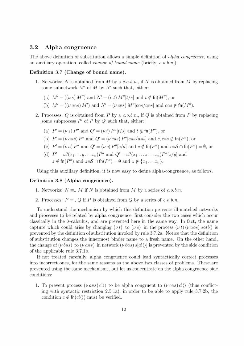
3.2 Alpha congruence

The above definition of substitution allows a simple definition of alpha congruence, usingan auxiliary operation, called change of bound name (briefly, c.o.b.n.).

Definition 3.7 (Change of bound name).

1. Networks: N is obtained from M by a c.o.b.n., if N is obtained from M by replacingsome subnetwork M ′ of M by N ′ such that, either:

(a) M ′ = ((ν s) M ′′) and N ′ = (ν t) M ′′[t/s] and t /∈ fn(M ′′), or

(b) M ′ = ((ν a@s) M ′) and N ′ = (ν c@s) M ′′[c@s/a@s] and c@s /∈ fn(M ′′).

2. Processes: Q is obtained from P by a c.o.b.n., if Q is obtained from P by replacingsome subprocess P ′ of P by Q′ such that, either:

(a) P ′ = (ν s) P ′′ and Q′ = (ν t) P ′′[t/s] and t /∈ fn(P ′′), or

(b) P ′ = (ν a@s) P ′′ and Q′ = (ν c@s) P ′′[c@s/a@s] and c, c@s /∈ fn(P ′′), or

(c) P ′ = (ν a) P ′′ and Q′ = (ν c) P ′′[c/a] and c /∈ fn(P ′′) and c@S ∩ fn(P ′′) = ∅, or

(d) P ′ = u?(x1 . . . y . . . xn)P ′′ and Q′ = u?(x1 . . . z . . . xn)P ′′[z/y] and

z /∈ fn(P ′′) and z@S ∩ fn(P ′′) = ∅ and z /∈ {x1 . . . xn}.

Using this auxiliary definition, it is now easy to define alpha-congruence, as follows.

Definition 3.8 (Alpha congruence).

1. Networks: N ≡α M if N is obtained from M by a series of c.o.b.n.

2. Processes: P ≡α Q if P is obtained from Q by a series of c.o.b.n.

To understand the mechanism by which this definition prevents ill-matched networksand processes to be related by alpha congruence, first consider the two cases which occurclassically in the λ-calculus, and are prevented here in the same way. In fact, the namecapture which could arise by changing (ν t) to (ν s) in the process (ν t) (ν a@s) a@t!〈〉 isprevented by the definition of substitution invoked by rule 3.7.2a. Notice that the definitionof substitution changes the innermost binder name to a fresh name. On the other hand,the change of (ν b@s) to (ν a@s) in network (ν b@s) s[a!〈〉] is prevented by the side conditionof the applicable rule 3.7.1b.

If not treated carefully, alpha congruence could lead syntactically correct processesinto incorrect ones, for the same reasons as the above two classes of problems. These areprevented using the same mechanisms, but let us concentrate on the alpha congruence sideconditions:

1. To prevent process (ν a@s) c!〈〉 to be alpha congruent to (ν c@s) c!〈〉 (thus conflict-ing with syntactic restriction 2.5.1a), in order to be able to apply rule 3.7.2b, thecondition c /∈ fn(c!〈〉) must be verified.

12

[SN-ALPHA] N ≡ M if N ≡α M

[SN-ASSO] ((N ‖M) ‖M ′) ≡ (M ‖ (N ‖M ′))[SN-COMM] (M ‖N) ≡ (N ‖M)[SN-NEUT] (N ‖ 0) ≡ N

[SN-SCOP] ((ν g) N) ‖M ≡ (ν g) (N ‖M) if g /∈ fn(M)[SN-RESO] (ν g) (ν h) N ≡ (ν h) (ν g) N if g /∈ names(h) and h /∈ names(g)[SN-RESZ] (ν g)0 ≡ 0

[SN-SCOS1] (ν r) s[P ] ≡ s[(ν r) P ] if r 6= s[SN-SCOS2] (ν a@r) s[P ] ≡ s[(ν a@r) P ] if a /∈ fn(P )[SN-SCOS3] (ν a@s) s[P ] ≡ s[(ν a) P ] if a@S ∩ fn(P ) = ∅[SN-ROUT] (s[P ] ‖ s[Q]) ≡ s[P |Q]

[SN-INAC] s[0] ≡ 0

[SN-MIGO] s[a@s!〈v〉] ≡ s[a!〈v〉][SN-MIGI] s[a@s?(x)P ] ≡ s[a?(x)P ]

Figure 7: Structural congruence on networks.

2. Similarly, to prevent process (ν a) c@s!〈〉 to be alpha congruent to (ν c) c@s!〈〉 (violat-ing syntactic restriction 2.5.1b), in order to be able to apply rule 3.7.2c, the conditionc@S ∩ fn(c@s!〈〉) = ∅ must be verified.

The following result ensures that the alpha-congruence relation is free of such problems.

Proposition 3.9 (Alpha congruence preserves the free names and the syntacticrestrictions). Let X and Y be both either networks or processes.

1. If X ok and X ≡α Y , then fn(X) = fn(Y ).

2. If X ok and X ≡α Y , then Y ok.

Proof. Both proofs use the name replacement version of Proposition 3.5 for a verifica-tion on each case of c.o.b.n.. Note that all the substitutions involved in the definition ofc.o.b.n. are name replacements. Furthermore, the second proof uses the name replacementversion of Proposition 3.6. Check the details in page 55.

3.3 Structural congruence

As usual in process calculi, we define the operational semantics of lsdπ following a “chemicalstyle” [4], i.e., via two binary relations on entities: a static one—structural congruence—and a dynamic one—reduction.

13

[SP-ALPHA] P ≡ Q if P ≡α Q

[SP-ASSO] ((P |Q) |R) ≡ (P | (Q |R))

[SP-COMM] (P |Q) ≡ (Q | P )

[SP-NEUT] (P | 0) ≡ P

[SP-SCOP1] ((ν s) P ) |Q ≡ (ν s) (P |Q) if s /∈ fn(Q)[SP-SCOP2] ((ν a@s) P ) |Q ≡ (ν a@s) (P |Q) if a, a@s /∈ fn(Q)[SP-SCOP3] ((ν a) P ) |Q ≡ (ν a) (P |Q) if ({a} ∪ a@S) ∩ fn(Q) = ∅[SP-RESO1] (ν g) (ν h) P ≡ (ν h) (ν g) P if g /∈ names(h) and h /∈ names(g)[SP-RESO2] (ν a) (ν s) P ≡ (ν s) (ν a) P if a@s /∈ fn(P )[SP-RESO3] (ν a) (ν u) P ≡ (ν u) (ν a) P if u /∈ a@S[SP-RESZ] (ν n)0 ≡ 0

Figure 8: Structural congruence on processes.

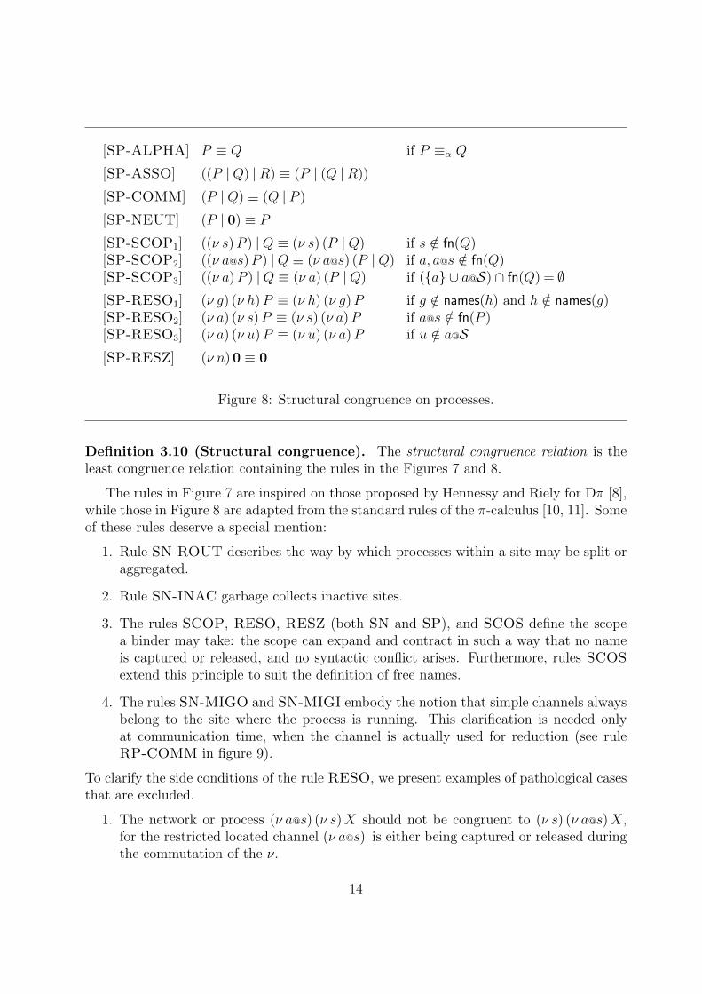
Definition 3.10 (Structural congruence). The structural congruence relation is theleast congruence relation containing the rules in the Figures 7 and 8.

The rules in Figure 7 are inspired on those proposed by Hennessy and Riely for Dπ [8],while those in Figure 8 are adapted from the standard rules of the π-calculus [10, 11]. Someof these rules deserve a special mention:

1. Rule SN-ROUT describes the way by which processes within a site may be split oraggregated.

2. Rule SN-INAC garbage collects inactive sites.

3. The rules SCOP, RESO, RESZ (both SN and SP), and SCOS define the scopea binder may take: the scope can expand and contract in such a way that no nameis captured or released, and no syntactic conflict arises. Furthermore, rules SCOSextend this principle to suit the definition of free names.

4. The rules SN-MIGO and SN-MIGI embody the notion that simple channels alwaysbelong to the site where the process is running. This clarification is needed onlyat communication time, when the channel is actually used for reduction (see ruleRP-COMM in figure 9).

To clarify the side conditions of the rule RESO, we present examples of pathological casesthat are excluded.

1. The network or process (ν a@s) (ν s) X should not be congruent to (ν s) (ν a@s) X,for the restricted located channel (ν a@s) is either being captured or released duringthe commutation of the ν.

14

2. The process (ν a) (ν s) a@s!〈〉 obviously should not be congruent to (ν s) (ν a) a@s!〈〉,since the latter process is not ok.

3. The process (ν a) (ν a@s) a@s!〈〉 should not be congruent to (ν a@s) (ν a) a@s!〈〉, andsimilarly, (ν a@s) (ν a) a!〈〉 should not be congruent to (ν a) (ν a@s) a!〈〉, since in bothcases the resulting processes are not ok.

Proposition 3.11 (Structural congruence preserves the free names and the syn-tactic restrictions). Let X and Y both be either networks or processes.

1. If X ok and X ≡ Y , then fn(X) = fn(Y ).

2. If X ok and X ≡ Y , then Y ok.

Proof. Both proofs perform a verification on each rule of structural congruence. In theprocess of proving this proposition, the side conditions of the mentioned rules may be un-derstood. The cases of the ALPHA rules follow from Proposition 3.9. Check the detailsin page 60.

3.4 Simultaneous substitutions and name translation

Since the calculus is polyadic, it is necessary to substitute several names at a time.

Definition 3.12 (Simultaneous substitutions). Consider two subsets {u1, . . . , un} and{v1, . . . , vn} of C, such that u1, . . . , un are pairwise distinct. Then {v1/u1, . . . , vn/un} is aset of simultaneous substitutions. The result of applying this set of substitutions to P is

P{v1/u1, . . . , vn/un}def=

{P [v1/u1] · · · [vn/un] if {u} ∩ {v}= ∅ ,P [w1/u1] · · · [wn/un][v1/w1] · · · [vn/wn] otherwise,

where w1, . . . , wn are fresh.

Notation 3.13 (Set of simultaneous substitutions). Let {v/x} abv= {v1/x1, . . . , vn/xn}

denote a set of simultaneous substitutions.

One can easily show that the order in which the substitutions in these sets are writtenis irrelevant to the result.

Proposition 3.14 (Commutativity in a set of simultaneous substitutions).P{v1/u1, . . . , vn/un} = P{v′1/u′1, . . . v′n/u′n} modulo c.o.b.n., where {v′1/u′1, . . . v′n/u′n} is apermutation of {v1/u1, . . . , vn/un}.

Proof. By a simple induction on the cardinality of the set.

Both the communication and the migration primitives that we present below, are defined

15

using the above notion of set of simultaneous substitutions. Notice that, in order to avoidname capture and release, as well as the emergence of syntactic errors, renaming of boundnames may occur. This may be seen as an “automatic alpha-conversion” that enablessubstitution to be a total function.

To keep channels “local by default”, when migrating process P from site r to site s, thefree channels of P must be renamed accordingly: thus simple channels become explicitlylocated at r; channels located at s become simple (dropping the @s part); all other channelsremain unchanged.

Definition 3.15 (Name translation). Let A ⊆ N , A ∩ C = {a1, . . . , an} and A ∩ C@s ={b1@s, . . . , bm@s}. Then,

σ(A, r, s)def= {a1@r/a1, . . . , an@r/an, b1/b1@s, . . . , bm/bm@s} .

Notation 3.16 (Application of name translation to a process). Let Pσrs abbreviatethe result of applying name translation σ(fn(P ), r, s) to process P .

3.5 Reduction

We are finally in a position to define the reduction relation. Reduction contexts simplifythe presentation of the reduction relation.

Definition 3.17 (Reduction contexts).

E ::= [] | (E | P ) | (ν n) EF ::= [] | (F ‖N) | (ν g) F

Definition 3.18 (Reduction). The rules in the Figure 9 inductively define the reductionrelation on processes and networks.

Axiom RP-COMM is standard in the π-calculus [10, 11], the axioms RN-MIGO andRN-MIGI were proposed by Vasconcelos et al. for DiTyCO [14], and the remaining rulesin the Figure 9 were proposed by Amadio et al. for Dπ [2].

So far we have defined two main relations (structural congruence and reduction) thatallow us to rewrite programs and simulate their computation. The two main results of thissection guarantee that, during reduction, on the one hand the set of free names does notincrease, and on the other hand, syntactic correctness is preserved.

Proposition 3.19 (Reduction preserves the free names and the syntactic restric-tions). Let X and Y both be either networks or processes.

1. If X ok and X → Y , then fn(X) ⊇ fn(Y ).

2. If X ok and X → Y , then Y ok.

16

[RP-COMM] a?(x)P | a!〈v〉 → P{v/x}[RN-MIGO] r[a@s!〈v〉] → s[(a@s!〈v〉)σrs] r 6= s

[RN-MIGI] r[a@s?(x)P ] → s[(a@s?(x)P )σrs] r 6= s

[RP-CONT]P → Q

E[P ] → E[Q]

[RP-STR]P ≡ P ′ P ′ → Q′ Q′ ≡ Q

P → Q

[RN-SITE]P → Q

s[P ] → s[Q]

[RN-CONT]N → M

F [N ] → F [M ]

[RN-STR]N ≡ N ′ N ′ → M ′ M ′ ≡ M

N → M

Figure 9: Reduction rules.

Proof. Both proofs consist in an induction on the derivation of the reduction step. Thedelicate cases are the axioms of reduction RP-COMM, RN-MIGO and RN-MIGI. Anauxiliary lemma is useful: If A⊆N and Υ is a finite sequence of substitutions, then

AΥ = {mΥ | m ∈ A} ∪ sites({mΥ | m ∈ A}) .

Use Proposition 3.5 and the lemma to prove the first clause, and Proposition 3.6 to provethe second. The induction steps concerning rules STR use Proposition 3.11. In the casesof CONT a second induction on the structure of the contexts should be used. Check thedetails in page 72.

3.6 Examples

We proceed by presenting some examples of the use of the language. We omit the appli-cation of some rules, like SN-COMM and SP-COMM, and underline redexes.

1. As an academic example, consider a site s running two processes, P and Q, in parallel.Process P =(ν a) (b@t?(x)x?()0 |a?()0) is expecting a message at a channel b locatedat site t. Furthermore, site t is running a process ready to send a message on a local

17

channel with the same channel b.

s[(ν a) (b@t?(x)x?()0 | a?()0) |Q] ‖ t[b!〈a〉 | a@s!〈〉 | a!〈〉]

The sphere of action of P is restricted to the scope of the enfolding (ν a) , which isinternal to site s, but using SN-SCOS, we may extrude it to the network level.

≡ (ν a@s) (s[b@t?(x)(x?()0 | a?()0) |Q]) ‖ t[b!〈a〉 | a@s!〈〉 | a!〈〉]

In order for P to migrate to site t, where it can perform the communication, it mustbe isolated, so, using SN-ROUT, we separate the site s into two parts.

≡ (ν a@s) (s[b@t?(x)(x?()0 | a?()0)] ‖ s[Q]) ‖ t[b!〈a〉 | a@s!〈〉 | a!〈〉]

Process P is now ready to migrate (using RN-MIGI).

→ (ν a@s) (t[b?(x)(x?()0 | a@s?()0)] ‖ s[Q]) ‖ t[b!〈a〉 | a@s!〈〉 | a!〈〉]

Within the current scope of (ν a@s) , no communication can occur at channel b, eventhough the two process are located at site t. We wish to extrude the scope of (ν a@s)even further, to encompass all the fragments of site t. Since a∈fn(b!〈a〉), this will onlybe possible if we rename the bound a@s to a fresh name, say c@s, using SN-ALPHA.In this way, there will be no confusion between the channel currently named “a”, andother uses of the same name.

≡α (ν c@s) (t[b?(x)(x?()0 | c@s?()0)] ‖ s[Q][c@s/a@s]) ‖ t[b!〈a〉 | a@s!〈〉 | a!〈〉]

Now we are free to expand the scope of (ν c@s) (using SN-SCOP),

≡ (ν c@s) t[b?(x)(x?()0 | c@s?()0)] ‖ s[Q][c@s/a@s] ‖ t[b!〈a〉 | a@s!〈〉 | a!〈〉]

and with SN-ROUT, we merge the two fragments of site t.

≡ (ν c@s) t[b?(x)(x?()0 | c@s?()0) | b!〈a〉 | a@s!〈〉 | a!〈〉] ‖ s[Q][c@s/a@s]

Communication may now proceed.

→ (ν c@s) t[a?()0 | c@s?()0 | a@s!〈〉 | a!〈〉] ‖ s[Q][c@s/a@s]

Now observe which processes are entitled to communicate. Only one process reduc-tion is possible.

→ (ν c@s) t[c@s?()0 | a@s!〈〉] ‖ s[Q][c@s/a@s]

18

2. A remote procedure call as in reference [14]. The client at site s uses the channel pto invoke a procedure Q at site r with a local argument v (assume that a does notoccur free in Q), waits for the reply and continues with P . The reply carries a localname u, which is sent by procedure Q at the end of its computation.

s[(ν a) (p@r!〈v a〉 | a?(y)P )] ‖ r[p?(x r)Q] ≡ [(1)]

(ν a@s) s[p@r!〈v a〉] ‖ s[a?(y)P ] ‖ r[p?(x r)Q] → [RN-MIGO]

(ν a@s) r[p!〈v@s a@s〉] ‖ s[a?(y)P ] ‖ r[p?(x r)Q] ≡ [SN-ROUT]

(ν a@s) s[a?(y)P ] ‖ r[p?(x r)Q | p!〈v@s a@s〉] → [RP-COMM]

(ν a@s) s[a?(y)P ] ‖ r[Q{v@s a@s/x r}] . . . [Q reduces]

(ν a@s) s[a?(y)P ] ‖ r[a@s!〈u〉] → [RN-MIGO]

(ν a@s) s[a?(y)P ] ‖ s[a!〈u@r〉] ≡ [SN-ROUT]

(ν a@s) s[a?(y)P | a!〈u@r〉] → [RP-COMM]

(ν a@s) s[P{u@r/y}] ≡ [SN-SCOS]

s[(ν a) P{u@r/y}]

(1) SN-SCOS, SN-ROUT, and SN-SCOP.

3. A primitive for the migration of arbitrary processes, under the lexical scope regime.To send a process P from site r to site s, one creates a remote channel a@s (not freein P ), prefix P with a receptor on a@s and put in parallel an message to a@s.

go s.Pabv= r[(ν a@s) a@s?()P | a@s!〈〉] ≡ [SN-SCOP,SN-ROUT]

(ν a@s) r[a@s?()P ] ‖ r[a@s!〈〉] →2 [SN-MIGO,SN-MIGI]

(ν a@s) s[a?()Pσrs] ‖ s[a!〈〉] ≡ [SN-ROUT,SN-SCOP]

s[(ν a) a?()Pσrs | a!〈〉] → [SN-COMM]

s[Pσrs]

Notice that the process that ends up in site s is not P but P with names translatedby σ. Contrast with go s.P → s[P ] in Amadio et al. [2].

4. The creation of “subsites”. One may create a (logical) subsite and restrict its accessto authorized processes. Since the name of this subsite is private to the master site,external processes must be given its identity to migrate there. In the example below,site s creates a subsite r and a channel c@r, communicates this name to site t thatuses it to download process Q (where x /∈ fn(Q)) from the t to r.

s[(ν r) (ν c@r) a@t!〈c@r〉 | P ] ‖ t[a?(x)x?()Q |R] →(ν r) (ν c@r) s[P ] ‖ t[a!〈c@r〉 | a?(x)x?()Q |R] →

(ν r) (ν c@r) s[P ] ‖ t[c@r?()Q |R] →(ν r) (ν c@r) (r[c?()Qσtr] ‖ s[P ]) ‖ t[R]

19

5. The creation of channels “anywhere” in the network. Consider a server with address aat site s that provides some application, which requires some resources (say a privatename b). Both local and remote clients may download it, since process

s[a?(x)x?()((ν b) P ) | (a!〈c〉 | c!〈〉) | (a!〈c@r〉 | c@r!〈〉)]

reduces either to s[(ν b) P ] or to r[(ν b) P ] (consider that x does not occur free in P ).Therefore, the site where (ν b) P will end up in is determined only at run-time.

This example illustrates an advantage of maintaining both simple and located formsof channels. If we were not able to specify the creation of simple channels (like b),then, since we don’t allow the passing of site names, all the locations of restrictedchannels would be determined statically. At first it might seem as an entanglement,but we believe that, in result of this decision, we can do without the passing of sites.

6. The creation of remote channels might be an undesirable operation. A possibilityis to disallow the (ν a@s) P constructor. Then we would only be able to migrateprocesses onto sites on which we know a friend that lends new channels (this is theapproach of reference [14]). Below, site r knows friend@s, asks for a new channel c(at s), and prefixes the process to migrate P at the new channel c@s.

(ν friend@s) r[(ν a) a?(x)x?()P | friend@s!〈a〉] ‖ s[friend?(x)((ν c) x!〈c〉 | c!〈〉)] →

(ν friend@s, a@r) r[a?(x)x?()P ] ‖ s[friend!〈a@r〉 | friend?(x)((ν c) x!〈c〉 | c!〈〉)] →

(ν a@r) r[a?(x)x?()P ] ‖ s[(ν c) a@r!〈c〉 | c!〈〉] →

(ν c@s) r[(ν a) a?(x)x?()P | a!〈c@s〉] ‖ s[c!〈〉)] →(ν c@s) r[c@s?()P ] ‖ s[c!〈〉)]

At this point c@s?()P may migrate to the friend’s site s, where a trigger c!〈〉 awaits.

(ν c@s) r[c@s?()P ] ‖ s[c!〈〉)] →

s[(ν c) c?()Pσrs | c!〈〉)] →

s[Pσrs]

The six reduction steps may be classified as three remote operations, each composedof migration followed by local reduction.

Some of the features described above should be carefully used. Type systems may beused to control and discipline the behavior of programs. The following section presents afirst system, a very basic one still not addressing security issues, but already ensuring theabsence of run-time errors.

20

4 The type system

This section presents the syntax of types, and a type checking system for lsdπ. Thesystem is a straightforward extension of that for the simply typed π-calculus [13], butalso borrowing ideas from that of Amadio et al.’s dπr

1 [2]; it assumes types for sites only(types for channels are taken from that of the site the channel belongs to), and enjoyssubject-reduction.

An essential ingredient of dπr1, a receptive and asynchronous version of Dπ, is the

type system, a simplified version of that of Hennessy and Riely [8], although it types lessprocesses (but a simple extension of the notion of type would probably lead to equivalentsystems). Types of lsdπ are a subset of those of dπr

1: simply remove the located type γ@,as a located channel may substitute a simple channel. The typing rules were adapted totake into consideration the lexical scope of channels.

Definition 4.1 (Types). Let n ≥ 0 and let a1, . . . , an and also s1, . . . , sn be pairwisedistinct.

Channel types, γ ::= Ch(γ1, . . . , γn)

Site types, ϕ ::= {a1:γ1, . . . , an:γn}Typings, Γ ::= {s1:ϕ1, . . . , sn:ϕn}

We have channel types (those of simple and located channels), and site types (those ofsites). A site type is a partial function from channels into channel types. A typing is apartial function from sites into site types.

Notation 4.2. 1. Let F, G be maps. The domain of F is written dom(F ); the mapobtained from F by removing x from its domain is denoted by F \ x. The disjointunion of F and G is denoted by F ]G.

2. Consider the union of typing assumptions Γ+∆ defined pointwise as, for all s∈dom(Γ)and for all a ∈ Γ(s) ∩∆(s):

(Γ + ∆)(s)def=

Γ(s), if s ∈ Γ \ dom(∆) or Γ(s) = ∆(s),Γ(s) ∪∆(s), if s ∈ dom(Γ) ∩ dom(∆) and Γ(s)(a) = ∆(s)(a),∆(s), if s ∈ dom(∆) \ dom(Γ).

Notice that this operation is not defined if Γ(s)(a) 6= ∆(s)(a).

The type system uses three kinds of judgments:

1. Γ`s v:τ , that types names, locations variables, and process variables v at site s, withtypes τ , according to the typing assumption Γ;

2. Γ`s P , saying that process P at site s conforms to the typing assumption Γ;

3. Γ`N , saying that network N conforms to typing assumption Γ.

21

TS-LCh Γ`r a@s:Γ(s)(a) TS-SCh Γ`s a:Γ(s)(a)

TS-UniΓ`s n1:γ1 ∆`s n2:γ2

Γ + ∆`s ˜n1n2:γ1γ1

Figure 10: Typing channels and sites.

TP-OutlΓ`r v:γ

Γ + {s:{a:Ch(γ)}} `r a@s!〈v〉TP-Outs

Γ`s a@s!〈v〉Γ`s a!〈v〉

TP-InplΓ ] {r:{x:γ}} `r P

Γ + {s:{a:Ch(γ)}} `r a@s?(x)PTP-Inps

Γ`s a@s?(x)P

Γ`s a?(x)P

TP-ParΓ`s P Γ`s Q

Γ`s (P |Q)TP-Resn

Γ ] {s:ϕ} `s P

Γ`s (ν s) P

TP-ReslΓ ] {s:{a:γ} ] ϕ} `r P

Γ ] {s:ϕ} `r (ν a@s) PTP-Ress

Γ`s (ν a@s) P

Γ`s (ν a) P

TP-WeakΓ`s P

Γ + ∆`s PTP-Nil ∅ `s 0

Figure 11: Typing processes.

Definition 4.3 (lsdπ type system). The rules in Figures 10, 11, and 12 inductivelydefine the type system of lsdπ.

The main result is the preservation of network typability under reduction, a propertyusually know as subject reduction. The following results break the ground for it.

Definition 4.4 (Substitution on typings). 1. A substitution of channels in a typingis a function defined, when x ∈ dom(Γ(s)), by the following rule:

Γ[a@r/x@s]def=

{{s:Γ(s) \ x} ∪ {r:{a:Γ(s)(x)}+ Γ(r)} ∪ Γ \ s \ r if r 6= s ;{s:Γ(s) \ x}+ {s:{a:Γ(s)(x)}} ∪ Γ \ s otherwise .

2. A substitution of sites in a typing is a function defined, when r ∈ dom(Γ), by rule:

Γ[s/r]def= Γ \ r + {s:Γ(r)}.

22

TN-NetΓ`s P

Γ` s[P ]TN-Nil ∅ `0 TN-Resn

Γ ] {s:ϕ} `N

Γ` (ν s) N

TN-ReslΓ ] {s:{a:γ} ] ϕ} `N

Γ ] {s:ϕ} ` (ν a@s) NTN-Par

Γ`N Γ`M

Γ` (N ‖M)

Figure 12: Typing networks.

Since this definition uses the union of typings, Γ[a@r/x@s] is not defined if a∈dom(Γ(r))and Γ(r)(a) 6=Γ(s)(x), and Γ[s/r] is not defined if s∈dom(Γ) and Γ(r) 6=Γ(s). The followingresult assures that the definition of substitution of channels in a typing is correct.

Proposition 4.5 (Substitution on typings). Consider ∆def= Γ[a@r/x@s] defined. Then:

1. x 6∈ dom(∆(s)) and ∆ \ s \ r = Γ \ s \ r;

2. if r 6= s then ∆(s) = Γ(s) \ x, otherwise ∆(s) \ a = Γ(s) \ x;

3. a ∈ dom(∆(r)) and ∆(r)(a) = Γ(s)(x), and if a ∈ dom(Γ(r)) then Γ(r)(a) = Γ(s)(x).

Proof. Follows easily from the definitions of substitution on and union of typings.

Since our calculus is polyadic, we are interested in simultaneous substitutions.

Notation 4.6. Let v@s be a@s if v = a, and v otherwise. Consider the simultaneous sub-stitution on typings Γ{v@s/x@s} defined similarly to the respective definition on processes(cf. Definition 3.12).

Lemma 4.7 (Simultaneous substitution). Let Γ`s P , and consider that x∈ fn(P ) butx@S ∩ fn(P ) = ∅. Then, Γ{v@s/x@s} `s P{v/x}.

Proof. Notice that Γ{v@s/x@s} is only defined when Γ(s)(v)=Γ(s)(x). The proof consistsin an induction on the length of v, using the following auxiliary result, which is proved byinduction on the derivation of the judgment Γ[a@r/x@s]`s P [a@r/x]:

Let Γ`s P , and consider that x ∈ fn(P ) but x@S ∩ fn(P ) = ∅. Then,

1. Γ[a@r/x@s]`s P [a@r/x], for all r, s; and

2. Γ[a@s/x@s]`s P [a/x], when r = s.

A detailed proof can be found in page 83.

The main result of this section states that reduction preserves the typability of a pro-cess. The lemma above is necessary when reduction results from communication. Whenreduction results from migration, apply the following lemma.

23

Lemma 4.8 (Channel translation). If Γ ] {s:{a:Ch(γ)}} ] {r:{x:γ}} `r P , thenΓ + {s:{a:Ch(γ), x:γ}} `s Pσ(fn(a@s?(x)P ), r, s).

Proof. The proof follows on by induction on the derivation of the judgment.

We are finally in a position to ensure the preservation of typability by reduction.

Theorem 4.9 (Subject reduction).

1. If Γ`s P and P → Q, then ∆`s Q, for some ∆.

2. If Γ`N and N → M , then ∆`M , for some ∆.

Proof. The proof consists of inductions on the derivations of P → Q and of N → M . Asusual, we use a lemma stating that structural congruence also preserves typability. Thebase case in the derivation of P → Q is when the last rule is RP-COMM. Use Lemma 4.7.There are two base cases to consider in the derivation of N → M :

1. Case the last rule is RN-MIGO—apply the Definition 3.15 and the typing rulesTP-Outl and TP-Outs subsequently.

2. Case the last rule is RN-MIGI—use then the Lemma 4.8.

The cases of the induction steps are straightforward.

5 Comparisons and Further work

The closest calculus to lsdπ is Dπ. The main differences are:

1. the latter has a general migration primitive that sends arbitrary processes to remotesites, while the former only migrates messages and receptors;

2. in the latter channels are global (do not belong to a specific site), while in the formerchannels are local (each belong to some site, and if s and r both have a channel a,the a of s is different from the a of r);

3. in the latter sites are first-class citizens, being passed around, while in the formerthey are not.

We expect that the choices made in lsdπ do not result in loss of expressiveness, whilegaining simplicity. Possible differences of expressive power in the semantics of these twocalculi are under investigation. Different models of distribution provide for an explicitmigration primitive; it is unclear at the time of this writing whether explicit migrationmay be simulated by our primitives.

24

We envisage to allow messages to carry sites; substitution, as defined in section 2, isready for that. Different models of distribution provide for an explicit migration primitive;it is unclear at the time of this writing whether explicit migration may be simulated byour primitives. Finally, we would like to control unrestricted migration (cf. [8]), possiblyvia type systems.

Acknowledgments

This work started during a six months visit of Antonio Ravara to the Project MIMOSA atINRIA Sophia Antipolis, France, partially supported by a post-doctoral grant of the FrenchRNRT project MARVEL. The Portuguese PRAXIS XXI project DiCoMo was anothersource for financial support of the work. Thanks to Gerard Boudol, Ilaria Castellani,Matthew Hennessy, and Francisco Martins for several fruitful discussions. Thanks to AnaMatos for suggesting lsd (π).

References

[1] Roberto M. Amadio. On modelling mobility. Theoretical Computer Science, 240:147–176, 2000.

[2] Roberto M. Amadio, Gerard Boudol, and Cedric Lhoussaine. The receptive distributedπ-calculus. Rapport de Recherche 4080, INRIA Sophia-Antipolis, 2000. A preliminaryversion in FST/TCS’99, LNCS 1738.

[3] Henk Barendregt. The Lambda Calculus - Its Syntax and Semantics. North-Holland,1981 (1st ed.), revised 1984.

[4] Gerard Berry and Gerard Boudol. The chemical abstract machine. Theoretical Com-puter Science, 96:217–248, 1992.

[5] Luca Cardelli. A language with distributed scope. In ACM, editor, POPL’95: 22ndAnnual ACM Symposium on Principles of Programming Languages (San Francisco,CA, U.S.A.), pages 286–297. ACM Press, 1995.

[6] Luca Cardelli and Andrew D. Gordon. Mobile ambients. In Maurice Nivat, editor,Proceedings of FoSSaCS ’98, volume 1378 of Lecture Notes in Computer Science, pages140–155. Springer-Verlag, 1998.

[7] Cedric Fournet, Georges Gonthier, Jean-Jacques Levy, Luc Maranget, and DidierRemy. A calculus of mobile agents. In CONCUR’96, volume 1119 of Lecture Notes inComputer Science, pages 406–421. Springer-Verlag, 1996.

25

[8] Matthew Hennessy and James Riely. Resource access control in systems of mobileagents. In HLCL’98, volume 16 (3) of Electronic Notes in Theoretical Computer Sci-ence. Elsevier Science Publishers, 1998. Full version as CogSci Report 2/98, Universityof Sussex, Brighton, U. K., 1998.

[9] J. Roger Hindley and Jonathan P. Seldin. Introduction to Combinators and λ-Calculus.Cambridge University Press, 1986.

[10] Robin Milner. The polyadic π-calculus: A tutorial. In Logic and Algebra of Specifi-cation, volume 94 of Series F. Springer-Verlag, 1993. Available as Technical ReportECS-LFCS-91-180, University of Edinburgh, U. K., 1991.

[11] Robin Milner, Joachim Parrow, and David Walker. A calculus of mobile processes,part I/II. Journal of Information and Computation, 100:1–77, 1992. Available asTechnical Reports ECS-LFCS-89-85 and ECS-LFCS-89-86, University of Edinburgh,U. K., 1989.

[12] Peter Sewell, Pawel Wojciechowski, and Benjamin C. Pierce. Location independencefor mobile agents. In Internet Programming Languages, volume 1686 of Lecture Notesin Computer Science. Springer-Verlag, 1999.

[13] Vasco T. Vasconcelos and Kohei Honda. Principal typing schemes in a polyadic π-calculus. In Eike Best, editor, Proceedings of CONCUR ’93, volume 715 of LectureNotes in Computer Science, pages 524–538. Springer-Verlag, 1993.

[14] Vasco T. Vasconcelos, Luıs Lopes, and Fernando Silva. Distribution and mobility withlexical scoping in process calculi. In HLCL’98, volume 16 (3) of Electronic Notes inTheoretical Computer Science. Elsevier Science Publishers, 1998.

26

A Proofs

A.1 Results on the operational semantics

Notation A.1 (Useful sets). In this section, the following abbreviations are used withrespect to the notation defined in Notation 2.2. Here, the use of channels of the form @sis to be interpreted as “any channel located at the site s”. If used inside “{}”, as in { @s},the resulting set is an abbreviation for C@s. If used as an element of a set, as in @s, itrepresents an arbitrary element of C@s. Furthermore, A@s is not used as in Notation 2.2,but is used, instead, in place of locate(A, s).

Lemma A.2 (Easy auxiliary results).

1. For A1, . . . ,Ak ⊆N , (A1 ∪ . . . ∪ Ak)[n/m] = A1[n/m] ∪ . . . ∪ Ak[n/m].

2. For X ok, if a@t ∈ fn(X) then t ∈ fn(X). Consequently, sites(fn(X)) ⊆ fn(X).

3. For X ok and [n/m] a replacement, fn(X)[n/m] = {m1[n/m] | m1 ∈ fn(X)}.

4. If A⊆N , and Υ is a finite sequence of substitutions, thenAΥ = {m1Υ | m1 ∈ A} ∪ sites({m1Υ | m1 ∈ A}) .

Proof of Lemma. These proofs are omitted, since they consist in straightforward appli-cations of the definitions.

Proposition A.3 (Substitution commutes with the free names). Let Υ be a finitesequence of substitutions.

1. If Υ is a name replacement, then fn(XΥ) = fn(X)Υ.

2. If Υ is a name instantiation, then fn(PΥ) = fn(P )Υ.

3. If Υ is a name translation, then fn(PΥ) ⊆ fn(P )Υ.

Proof of Proposition A.3.1 and A.3.2. The proof consists of an induction over thestructure of the entities. At the Process level, we provide both Propositions A.3.1 and A.3.2at the same time. No confusion should arise from this choice, since it is clear from thecontext whether we are verifying a name replacement or a name instantiation. Obviously,at the Network level, it suffices to consider A.3.1.

For each case, it is necessary to perform a mathematical induction over the length ofthe sequence of substitutions. Therefore we will be looking at nested induction proof.We use the following abbreviations to refer to the invocation of induction base (i.b.) andhypothesis (i.h.) and distinguish between the two levels of induction.

- i.h.1, i.b.1abv= i.h. and i.b. of the basic structural induction of this proof.

27

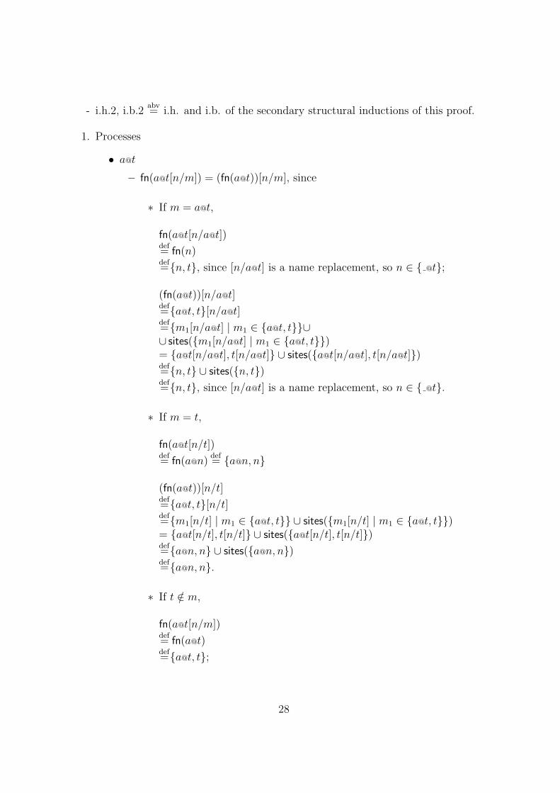
- i.h.2, i.b.2abv= i.h. and i.b. of the secondary structural inductions of this proof.

1. Processes

• a@t

– fn(a@t[n/m]) = (fn(a@t))[n/m], since

∗ If m = a@t,

fn(a@t[n/a@t])def= fn(n)def={n, t}, since [n/a@t] is a name replacement, so n ∈ { @t};

(fn(a@t))[n/a@t]def={a@t, t}[n/a@t]def={m1[n/a@t] | m1 ∈ {a@t, t}}∪∪ sites({m1[n/a@t] | m1 ∈ {a@t, t}})= {a@t[n/a@t], t[n/a@t]} ∪ sites({a@t[n/a@t], t[n/a@t]})def={n, t} ∪ sites({n, t})def={n, t}, since [n/a@t] is a name replacement, so n ∈ { @t}.

∗ If m = t,

fn(a@t[n/t])def= fn(a@n)

def= {a@n, n}

(fn(a@t))[n/t]def={a@t, t}[n/t]def={m1[n/t] | m1 ∈ {a@t, t}} ∪ sites({m1[n/t] | m1 ∈ {a@t, t}})= {a@t[n/t], t[n/t]} ∪ sites({a@t[n/t], t[n/t]})def={a@n, n} ∪ sites({a@n, n})def={a@n, n}.

∗ If t /∈ m,

fn(a@t[n/m])def= fn(a@t)def={a@t, t};

28

(fn(a@t))[n/m]def={a@t, t}[n/m]def={m1[n/m] | m1 ∈ {a@t, t}} ∪ sites({m1[n/m] | m1 ∈ {a@t, t}})= {a@t[n/m], t[n/m]} ∪ sites({a@t[n/m], t[n/m]})def={a@t, t} ∪ sites({a@t, t})def={a@t, t}.

– fn(a@t[n1/m1] . . . [nf/mf ])By definition, a@t[n1/m1] ∈ C@S,= (i.h.2) fn(a@t[n1/m1])[n2/m2] . . . [nf/mf ]= (i.b.2) (fn(a@t))[n1/m1] . . . [nf/mf ]

• a

– fn(a[n/m]) = (fn(a))[n/m], for

∗ If m = a,

fn(a[n/a])def= fn(n)def={n} ∪ sites({n});

(fn(a))[n/a]def={m1[n/a] | m1 ∈ fn(a)} ∪ sites({m1[n/a] | m1 ∈ fn(a)})def={a[n/a]} ∪ sites({a[n/a]})def={n} ∪ sites({n}).

∗ If m 6= a,

fn(a[n/m])def= fn(a)def={a};

(fn(a))[n/m]def={m1[n/m] | m1 ∈ fn(a)} ∪ sites({m1[n/m] | m1 ∈ fn(a)})def={a[n/m]} ∪ sites({a[n/m]})def={a}.

– fn(a[n1/m1] . . . [nf/mf ])By definition, a[n1/m1] ∈ Chans. If a[n1/m1] ∈ C use i.h.2, and if a[n1/m1] ∈

29

C@S use the previous case.

= fn(a[n1/m1])[n2/m2] . . . [nf/mf ]= (i.b.2) (fn(a))[n1/m1] . . . [nf/mf ].

• s

– fn(s[n/m]) = (fn(s))[n/m], for

∗ If m = s,

fn(s[n/s])def= fn(n)def={n}, since [n/s] is a name replacement, then n ∈ S;

(fn(s))[n/s]def={m1[n/s] | m1 ∈ fn(s)} ∪ sites({m1[n/s] | m1 ∈ fn(s)})def={s[n/s]} ∪ sites({s[n/s]})def={n} ∪ sites({n})def={n}, since [n/s] is a name replacement, then n ∈ S.

∗ If m 6= s,

fn(s[n/m])def= fn(s)def={s};

(fn(s))[n/m]def={m1[n/m] | m1 ∈ fn(s)} ∪ sites({m1[n/m] | m1 ∈ fn(s)})def={s[n/m]} ∪ sites({s[n/m]})def={s}.

– fn(s[n1/m1] . . . [nf/mf ]).By definition s[n1/m1] ∈ S,= (i.h.2) fn(s[n1/m1])[n2/m2] . . . [nf/mf ]= (i.b.2) (fn(s))[n1/m1] . . . [nf/mf ].

• 0

30

– fn(0[n/m]) = (fn(0))[n/m], for

fn(0[n/m])def= fn(0)def=∅;

(fn(0))[n/m]def=∅[n/m]= ∅.

– fn(0[n1/m1] . . . [nf/mf ])def= fn(0[n2/m2] . . . [nf/mf ])= (i.h.2) fn(0)[n2/m2] . . . [nf/mf ]= (i.b.2) fn(0)[n1/m1] . . . [nf/mf ]

• u!〈n〉

– fn(u!〈n〉[n/m]) = (fn(u!〈n〉))[n/m], for

fn((u!〈n〉)[n/m])def= fn(u[n/m]!〈n1[n/m] . . . nf [n/m]〉)def= fn(u[n/m]) ∪ fn(n1[n/m]) ∪ . . . ∪ fn(nf [n/m])= (i.h.1) fn(u)[n/m] ∪ fn(n1[n/m]) ∪ . . . ∪ fn(nf )[n/m];

(fn(u!〈n〉))[n/m]def=(fn(u) ∪ fn(n1) ∪ . . . ∪ fn(nf ))[n/m]= (Lemma A.2.1) fn(u)[n/m] ∪ fn(n1)[n/m] ∪ . . . ∪ fn(nf )[n/m].

– fn(u!〈n〉[n1/m1] . . . [nf/mf ]).Since by definition u!〈n〉[n1/m1] is of the form u′!〈n′n′〉,= (i.h.2) fn(u!〈n〉[n1/m1])[n2/m2] . . . [nf/mf ]= (i.b.2) (fn(u!〈n〉))[n1/m1] . . . [nf/mf ].

• P |Q

– fn((P |Q)[n/m]) = (fn(P |Q))[n/m], for

fn((P |Q)[n/m])def= fn((P )[n/m] | (Q)[n/m])

31

def= fn((P )[n/m]) ∪ fn((Q)[n/m])= (i.h.1) fn(P )[n/m] ∪ fn(Q)[n/m].

(fn(P |Q))[n/m]def=(fn(P ) ∪ fn(Q))[n/m]= (Lemma A.2.1) fn(P )[n/m] ∪ fn(Q)[n/m].

– fn((P |Q)[n1/m1] . . . [nf/mf ]).Since by definition (P |Q)[n1/m1] is of the form P ′ |Q′,= (i.h.2) fn(P [n1/m1] |Q[n1/m1])[n2/m2] . . . [nf/mf ]= (i.b.2) (fn(P |Q))[n1/m1] . . . [nf/mf ].

• (ν t) Q

– fn((ν t) Q[n/m]) = (fn((ν t) Q))[n/m], for

∗ If t ∈ m,

fn(((ν t) Q)[n/m])def= fn((ν t) Q)def= fn(Q) \ { @t, t}

(fn((ν t) Q))[n/m]def=(fn(Q) \ { @t, t})[n/m]def={m1[n/m] | m1 ∈ fn(Q) \ { @t, t}}∪∪ sites({m1[n/m] | m1 ∈ fn(Q) \ { @t, t}})def= fn(Q) \ { @t, t} ∪ sites(fn(Q) \ { @t, t}),because t /∈ m1 but t ∈ m= (Lemma A.2.2) fn(Q) \ { @t, t}

∗ If t /∈ m, and t /∈ n or m /∈ fn(Q)

fn(((ν t) Q)[n/m])def= fn((ν t) Q[n/m])def= fn(Q[n/m]) \ { @t, t}

(fn((ν t) Q))[n/m]def=(fn(Q) \ { @t, t})[n/m]def={m1[n/m] | m1 ∈ fn(Q) \ { @t, t}}∪∪ sites({m1[n/m] | m1 ∈ fn(Q) \ { @t, t}})

32

By hypothesis,

= {m1[n/m] | m1 ∈ fn(Q)} \ { @t, t}∪∪ sites({m1[n/m] | m1 ∈ fn(Q)}) \ { @t, t}def=(fn(Q)[n/m]) \ { @t, t}= (i.h.1) fn(Q[n/m]) \ { @t, t}

∗ If t /∈ m, and t ∈ n and m ∈ fn(Q), where s is fresh.

fn(((ν t) Q)[n/m])def= fn((ν s) Q[s/t][n/m])def= fn(Q[s/t][n/m]) \ { @s, s}

(fn((ν t) Q))[n/m]def=(fn(Q) \ { @t, t})[n/m]def={m1[n/m] | m1 ∈ fn(Q) \ { @t, t}}∪∪ sites({m1[n/m] | m1 ∈ fn(Q) \ { @t, t}})= (*) {m1[n/m] | m1 ∈ (fn(Q)[s/t]) \ { @s, s}}∪∪ sites({m1[n/m] | m1 ∈ (fn(Q)[s/t]) \ { @s, s}})

Since s is fresh, s /∈ n, m, thus= {m1[n/m] | m1 ∈ fn(Q)[s/t]} \ { @s, s}∪∪ sites({m1[n/m] | m1 ∈ fn(Q)[s/t]}) \ { @s, s}def=(fn(Q)[s/t][n/m]) \ { @s, s}= (i.h.1) fn(Q[s/t][n/m]) \ { @s, s} (i.h.1. may be used since [s/t] is aname replacement)

(*) ((fn(Q)[s/t]) \ { @s, s}def={m1[s/t] | m1 ∈ fn(Q)} \ { @s, s} ∪ sites({m1[s/t] | m1 ∈ fn(Q)}) \{ @s, s}def={m1 | m1 ∈ fn(Q)} \ { @t, t} ∪ sites({m1 | m1 ∈ fn(Q)}) \ { @t, t}= fn(Q) \ { @t, t}

– fn(((ν t) Q)[n1/m1] . . . [nf/mf ])

By definition ((ν t) Q)[n1/m1] is of the form (ν t′) Q′

= (i.h.2) fn(((ν t) Q)[n1/m1])[n2/m2] . . . [nf/mf ]= (i.b.2) (fn((ν t) Q))[n1/m1] . . . [nf/mf ]

33

• (ν a) Q

– fn((ν a) Q[n/m]) = (fn((ν a) Q))[n/m], since

∗ If m = a,

fn(((ν a) Q)[n/a])def= fn((ν a) Q)def= fn(Q) \ {a}

(fn((ν a) Q))[n/a]def=(fn(Q) \ {a})[n/a]def={m1[n/a] | m1 ∈ fn(Q) \ {a}} ∪ sites({m1[n/a] | m1 ∈ fn(Q) \ {a}})def= fn(Q) \ {a} ∪ sites(fn(Q) \ {a}), since m1 6= a= (Lemma A.2.2) fn(Q) \ {a}

∗ If m 6= a, and a /∈ n or m /∈ fn(Q)

fn(((ν a) Q)[n/m])def= fn((ν a) Q[n/m])def= fn(Q[n/m]) \ {a}

(fn((ν a) Q))[n/m]def=(fn(Q) \ {a})[n/m]def={m1[n/m] | m1 ∈ fn(Q) \ {a}} ∪ sites({m1[n/m] | m1 ∈ fn(Q) \ {a}})

By hypothesis,

def={m1[n/m] | m1 ∈ fn(Q)} \ {a} ∪ sites({m1[n/m] | m1 ∈ fn(Q)} \ {a})def=(fn(Q)[n/m]) \ {a}= (i.h.1) fn(Q[n/m]) \ {a}

∗ If m 6= a, and a ∈ n and m ∈ fn(Q), where b is fresh,

fn(((ν a) Q)[n/m])def= fn((ν b) Q[b/a][n/m])def= fn(Q[b/a][n/m]) \ {b}

(fn((ν a) Q))[n/m]

34

def=(fn(Q) \ {a})[n/m]def={m1[n/m] | m1 ∈ fn(Q) \ {a}}∪∪ sites({m1[n/m] | m1 ∈ fn(Q) \ {a}})= (*) {m1[n/m] | m1 ∈ fn(Q)[b/a]{b}}∪∪ sites({m1[n/m] | m1 ∈ fn(Q)[b/a]{b}})

Since b is fresh, b /∈ n, m, so= {m1[n/m] | m1 ∈ fn(Q)[b/a]} \ {b}∪∪ sites({m1[n/m] | m1 ∈ fn(Q)[b/a]}) \ {b}

def=(fn(Q)[b/a][n/m]) \ {b}= (i.h.1) fn(Q[b/a][n/m]) \ {b} (i.h.1. may be applied because [b/a] isreplacement.)

(*) ((fn(Q)[b/a]) \ {b}def={m1[b/a] | m1 ∈ fn(Q)} \ {b} ∪ sites({m1[b/a] | m1 ∈ fn(Q)}) \ {b}def={m1 | m1 ∈ fn(Q)} \ {a} ∪ sites({m1 | m1 ∈ fn(Q)}) \ {a}= fn(Q) \ {a}

– fn(((ν a) Q)[n1/m1] . . . [nf/mf ])

Since by definition ((ν a) Q)[n1/m1] is of the form (ν a′) Q′

= (i.h.2) fn(((ν a) Q)[n1/m1])[n2/m2] . . . [nf/mf ]= (i.b.2) (fn((ν a) Q))[n1/m1] . . . [nf/mf ]

• (ν a@t) Q

– fn((ν a@t) Q[n/m]) = (fn((ν a@t) Q))[n/m], for

∗ If m = a@t,

fn(((ν a@t) Q)[n/a@t])def= fn((ν a@t) Q)def= fn(Q) \ {a@t} ∪ {t}

(fn((ν a@t) Q))[n/a@t]def=(fn(Q) \ {a@t} ∪ {t})[n/a@t]def={m1[n/a@t] | m1 ∈ (fn(Q) \ {a@t} ∪ {t})}∪∪ sites({m1[n/a@t] | m1 ∈ (fn(Q) \ {a@t} ∪ {t})})

35

def= fn(Q) \ {a@t} ∪ {t} ∪ sites(fn(Q) \ {a@t} ∪ {t}), since m1 6= a@t butm = a@t= (Lemma A.2.2) fn(Q) \ {a@t} ∪ {t}

∗ If m = t,

fn(((ν a@t) Q)[n/t])def= fn((ν a@n) Q[n/t])def= fn(Q[n/t]) \ {a@n} ∪ {n}

(fn((ν a@t) Q))[n/t]def=(fn(Q) \ {a@t} ∪ {t})[n/t]def={m1[n/t] | m1 ∈ (fn(Q) \ {a@t} ∪ {t})}∪∪ sites({m1[n/t] | m1 ∈ (fn(Q) \ {a@t} ∪ {t})})def={m1[n/t] | m1 ∈ fn(Q) \ {a@t}} ∪ {n}∪∪ sites({m1[n/t] | m1 ∈ fn(Q) \ {a@t}} ∪ {n})def={m1 | m1 ∈ fn(Q)}\{a@n}∪{n}∪sites({m1 | m1 ∈ fn(Q)} \ {a@t} ∪ {n})= (fn(Q)[n/t]) \ {a@n} ∪ {n} ∪ sites((fn(Q)[n/t]) \ {a@n} ∪ {n})= (i.h.1) fn(Q[n/t]) \ {a@n} ∪ {n} ∪ sites(fn(Q[n/t]) \ {a@n})= (Lemma A.2.2) fn(Q[n/t]) \ {a@n} ∪ {n}

∗ If m 6= a@t, t, and n 6= a,a@t or m /∈ fn(M)

fn(((ν a@t) Q)[n/m])def= fn((ν a@t) Q[n/m])def= fn(Q[n/m]) \ {a@t} ∪ {t}

(fn((ν a@t) Q))[n/m]def=(fn(Q) \ {a@t} ∪ {t})[n/m]def={m1[n/m] | m1 ∈ (fn(Q) \ {a@t} ∪ {t})}∪∪ sites({m1[n/m] | m1 ∈ (fn(Q) \ {a@t} ∪ {t})})

By hypothesis,

def={m1[n/m] | m1 ∈ fn(Q)} \ {a@t} ∪ {t}∪∪ sites({m1[n/m] | m1 ∈ fn(Q)} \ {a@t} ∪ {t})= (fn(Q)[n/m]) \ {a@t} ∪ {t}= (i.h.1) fn(Q[n/m]) \ {a@t} ∪ {t}

∗ If m 6= a@t and m 6= t, and n ∈ {a, a@t} and m ∈ fn(M), where b is fresh

36

fn(((ν a@t) Q)[n/m])def= fn((ν b@t) M [b@t/a@t][n/m])def= fn(M [b@t/a@t][n/m]) \ {b@t} ∪ {t}

(fn((ν a@t) Q))[n/m]def=(fn(Q) \ {a@t} ∪ {t})[n/m]def={m1[n/m] | m1 ∈ (fn(Q) \ {a@t} ∪ {t})}∪∪ sites({m1[n/m] | m1 ∈ (fn(Q) \ {a@t} ∪ {t})})= (*) {m1[n/m] | m1 ∈ (fn(Q)[b@t/a@t]) \ {b@t}∪ ∪{t}}∪∪ sites({m1[n/m] | m1 ∈ (fn(Q)[b@t/a@t]) \ {b@t} ∪ {t}})

Since b is fresh, b /∈ n, m, and since m 6= t

= {m1[n/m] | m1 ∈ fn(Q)[b@t/a@t]} \ {b@t} ∪ {t}∪∪ sites({m1[n/m] | m1 ∈ fn(Q)[b@t/a@t]} \ {b@t} ∪ {t})def=(fn(Q)[b@t/a@t][n/m]) \ {b@t} ∪ {t}= (i.h.1) fn(Q[b@t/a@t][n/m]) \ {b@t}∪{t} (i.h.1. may be used because[b@t/a@t] is a name replacement)

(*) ((fn(Q)[b@t/a@t]) \ {b@t} ∪ {t}def={m1[b@t/a@t] | m1 ∈ fn(Q)} \ {b@t} ∪ {t}∪ ∪ts{m1[b@t/a@t] | m1 ∈ fn(Q)} \ {b@t} ∪ {t}

Since b is fresh, b@t /∈ fn(Q),

def={m1 | m1 ∈ fn(Q)}\{a@t}∪{t}∪sites({m1 | m1 ∈ fn(Q)})\{a@t}∪{t}= fn(Q) \ {a@t} ∪ {t}

– fn(((ν a@t) Q)[n1/m1] . . . [nf/mf ])

Since by definition ((ν a@t) Q)[n1/m1] is of the form (ν a′@t) Q′

= (i.h.2) fn(((ν a@t) Q)[n1/m1])[n2/m2] . . . [nf/mf ]= (i.b.2) (fn((ν a@t) Q))[n1/m1] . . . [nf/mf ]

• u?(a)Q

– fn(u?(a)Q[n/m]) = (fn(u?(a)Q))[n/m], for

∗ If m = ai and ai ∈ {a},

37

fn((u?(a)Q)[n/ai])def= fn(u[n/ai]?(a)Q)def= fn(Q) \ {a} ∪ {u} ∪ fn(u)

(fn(u?(a)Q))[n/ai]def=(fn(u) ∪ fn(Q) \ {a})[n/ai]= (Lemma A.2.1) fn(u)[n/m] ∪ (fn(Q) \ {a})[n/ai]def= fn(u)[n/ai] ∪ {m1[n/ai] | m1 ∈ fn(Q) \ {a}}∪∪ sites({m1[n/ai] | m1 ∈ fn(Q) \ {a}})def= fn(u)[n/m] ∪ fn(Q) \ {a} ∪ sites(fn(Q) \ {a}) since m1 /∈ {a}= (Lemma A.2.2) fn(u)[n/m] ∪ fn(Q) \ {a}= (i.h.1) fn(u[n/m]) ∪ fn(Q) \ {a}

∗ If m /∈ {a}, and ∀ai : ai /∈ n or m /∈ fn(Q)

fn((u?(a)Q)[n/m])def= fn(u[n/m]?(a)Q[n/m])def= fn(u[n/m]) ∪ fn(Q[n/m]) \ {a}

fn((u?(a)Q))[n/m]def=(fn(u) ∪ fn(Q) \ {a})[n/m]= (Lemma A.2.1) fn(u)[n/m] ∪ (fn(Q) \ {a})[n/m]def= fn(u)[n/m] ∪ {m1[n/m] | m1 ∈ fn(Q) \ {a}}∪∪ sites({m1[n/m] | m1 ∈ fn(Q) \ {a}})

By hypothesis,

def= fn(u)[n/m] ∪ {m1[n/m] | m1 ∈ fn(Q)} \ {a}∪∪ sites({m1[n/m] | m1 ∈ fn(Q)} \ {a}})def= fn(u)[n/m] ∪ (fn(Q)[n/m]) \ {a}= (i.h.1) fn(u[n/m]) ∪ fn(Q[n/m]) \ {a}

∗ If m /∈ {a}, and for some i : ai ∈ n and m ∈ fn(Q)

fn((u?(a)Q)[n/m])def= fn(u[n/m]?(a1 . . . b . . . an)Q[b/ai][n/m])def= fn(u[n/m]) ∪ fn(Q[b/ai][n/m]) \ {a1 . . . b . . . an}

fn((u?(a)Q))[n/m]

38

def=(fn(u) ∪ fn(Q) \ {a})[n/m]= (Lemma A.2.1) fn(u)[n/m] ∪ (fn(Q) \ {a})[n/m]def= fn(u)[n/m] ∪ {m1[n/m] | m1 ∈ fn(Q) \ {a}}∪∪ sites({m1[n/m] | m1 ∈ fn(Q) \ {a}})= (*) fn(u)[n/m] ∪ {m1[n/m] | m1 ∈ (fn(Q)[b/ai]) \ {a1 . . . b . . . an}}∪∪ sites({m1[n/m] | m1 ∈ (fn(Q)[b/ai]) \ {a1 . . . b . . . an}})

Since b is fresh, b /∈ n, m, so= fn(u)[n/m] ∪ {m1[n/m] | m1 ∈ (fn(Q)[b/ai])} \ {a1 . . . b . . . an}∪∪ sites({m1[n/m] | m1 ∈ (fn(Q)[b/ai])} \ {a1 . . . b . . . an})

def= fn(u)[n/m] ∪ (fn(Q)[b/ai][n/m]) \ {a1 . . . b . . . an}= (i.h.1) fn(u)[n/m]∪ fn(Q[b/ai][n/m]) \ {a1 . . . b . . . an} (i.h.1. may beused because [b/ai] is a name replacement)

(*) ((fn(Q)[b/ai]) \ {a1 . . . b . . . an}def={m1[b/ai] | m1 ∈ fn(Q)} \ {a1 . . . b . . . an}∪∪ sites({m1[b/ai] | m1 ∈ fn(Q)}) \ {a1 . . . b . . . an}def={m1 | m1 ∈ fn(Q)} \ {a}∪∪ sites({m1 | m1 ∈ fn(Q)}) \ {a}= (Lemma A.2.2) fn(Q) \ {a}

– fn((u?(a)Q)[n1/m1] . . . [nf/mf ])

Since by definition (u?(a)Q)[n1/m1] is of the form u′?(a′)Q′,

= (i.h.2) fn((u?(a)Q)[n1/m1])[n2/m2] . . . [nf/mf ]= (i.b.2) (fn(u?(a)Q))[n1/m1] . . . [nf/mf ]

• Networks

Note that, as mentioned in the beginning of the proof, from now on we considername replacement alone.

• s[Q]

– fn(s[Q][n/m]) = (fn(s[Q]))[n/m], for

∗ If m = a@s,

fn((s[Q])[b@s/a@s])

39

def= fn(s[(Q[b/a])[b@s/a@s]])def= fn((Q[b/a])[b@s/a@s])@s ∪ {s}

fn(s[Q])[b@s/a@s]def=(fn(Q)@s ∪ {s})[b@s/a@s]def=(Lemma A.2.3) {m1[b@s/a@s] | m1 ∈ (fn(Q)@s ∪ {s})}= {m1[b/a][b@s/a@s] | m1 ∈ fn(Q)}@s ∪ {s} (the substitution doesn’tchange s)def=(fn(Q)[b/a][b@s/a@s])@s ∪ {s}= (i.h.1) fn(Q[b/a][b@s/a@s])@s ∪ {s} (i.h.1. may be used because [b/a]and [b@s/a@s] are name replacements)

∗ If m = s,

fn((s[Q])[n/s])def= fn(n[Q[n/s]])def= fn(Q[n/s])@n ∪ {n}

fn(s[Q])[n/s]def=(fn(Q)@s ∪ {s})[n/s]def=(Lemma A.2.3) {m1[n/s] | m1 ∈ (fn(Q)@s ∪ {s})}= {m1[n/s] | m1 ∈ fn(Q)}@n ∪ {n}def= fn(Q)[n/s]@n ∪ {n}= (i.h.1) fn(Q[n/s])@n ∪ {n}

∗ If s /∈ m,

fn((s[Q])[n/m])def= fn(s[P [n/m]])def= fn(P [n/m])@s ∪ {s}

fn(s[Q])[n/m]def=(fn(Q)@s ∪ {s})[n/m]def=(Lemma A.2.3) {m1[n/m] | m1 ∈ (fn(Q)@s ∪ {s})}= {m1[n/m] | m1 ∈ fn(Q)}@s ∪ {s}def=(fn(Q)[n/m])@s ∪ {s}= (i.h.1) fn(Q[n/m])@s ∪ {s}

– fn((s[Q])[n1/m1] . . . [nf/mf ])

40

Since by definition (s[Q])[n1/m1] is of the form s′[Q′] then

= (i.h.2) fn((s[Q])[n1/m1])[n2/m2] . . . [nf/mf ]= (i.b.2) (fn(s[Q]))[n1/m1] . . . [nf/mf ]

• 0, M1 ‖M2, (ν a@t) M

As in the case for processes.

Proof of Proposition A.3.3. This proof is analogous to the previous one. Note that, bydefinition of X ok, the i.h. may be applied to all subterms of X.

1. Processes

• a

– fn(a[u/v]) = (fn(a))[u/v], for

∗ If v = a,

fn(a[u/a])def= fn(u)def={u} ∪ sites({u})

(fn(a))[u/a]def={m1[u/a] | m1 ∈ fn(a)} ∪ sites({m1[u/a] | m1 ∈ fn(a)})def={a[u/a]} ∪ sites({a[u/a]})def={u} ∪ sites({u})

∗ If v 6= a,

fn(a[u/v])def= fn(a)def={a}

(fn(a))[u/v]def={m1[u/v] | m1 ∈ fn(a)} ∪ sites({m1[u/v] | m1 ∈ fn(a)})

41

def={a[u/v]} ∪ sites({a[u/v]}) since v 6= adef={a}

∗ fn(a[u1/v1] . . . [uf/vf ])= (i.h.2) fn(a[u1/v1])[u2/v2] . . . [uf/vf ]= (i.b.2) (fn(a))[u1/v1] . . . [uf/vf ]

• s

– fn(s[u/v]) = (fn(s))[u/v], for

∗ Of course that v 6= s,

fn(s[u/v])def= fn(s)def={s}

(fn(s))[u/v]def={m1[u/v] | m1 ∈ fn(s)} ∪ sites({m1[u/v] | m1 ∈ fn(s)})def={s[u/v]} ∪ sites({s[u/v]})def={s}

– fn(s[u1/v1] . . . [uf/vf ])= (i.h.2) fn(s[u1/v1])[u2/v2] . . . [uf/vf ]= (i.b.2) (fn(s))[u1/v1] . . . [uf/vf ]

• a@t

– fn(a@t[u/v]) = (fn(a@t))[u/v], for

∗ If v = a@t, then u = a, since [u/v] is a name translation

fn(a@t[a/a@t])def= fn(a)def={a}

(fn(a@t))[a/a@t]def={a@t, t}[a/a@t]def={m1[a/a@t] | m1 ∈ {a@t, t}} ∪ sites({m1[a/a@t] | m1 ∈ {a@t, t}})= {a@t[a/a@t], t[a/a@t]} ∪ sites({a@t[a/a@t], t[a/a@t]})

42

def={a, t} ∪ sites({a, t})def={a, t}

∗ If t /∈ v,

fn(a@t[u/v])def= fn(a@t)def={a@t, t}

(fn(a@t))[u/v]def={a@t, t}[u/v]def={m1[u/v] | m1 ∈ {a@t, t}} ∪ sites({m1[u/v] | m1 ∈ {a@t, t}})= {a@t[u/v], t[u/v]} ∪ sites({a@t[u/m], t[u/v]})def={a@t, t} ∪ sites({a@t, t}) since t /∈ v,def={a@t, t}

– fn(a@t[u1/v1] . . . [uf/vf ])= (i.h.2) fn(a@t[u1/v1])[u2/v2] . . . [uf/vf ]= (i.b.2) (fn(a@t))[u1/v1] . . . [uf/vf ]

2. Networks

Note that the rest is analogous to Proof A.3.1, but u,v is used instead of m,n, andin place of the equality invoked by i.h.1, the ⊆ relation is used.

Proposition A.4 (Substitution preserves the syntactic restrictions). Let Υ be afinite sequence of substitutions.

1. If X ok and Υ is a name replacement, then XΥ ok.

2. If P ok and Υ is a name instantiation, then PΥ ok.

3. If P ok and Υ is a name translation, then PΥ ok.

Proof of Proposition A.4.1 and A.4.2. The proof consists of an induction over thestructure of the entities, supporting mathematical inductions over the length of the se-quence of substitutions. Again, proofs for Propositions A.4.1 and A.4.2 are presentedtogether. Moreover, Proposition A.3.1 is invoked in the cases where syntactic restrictionrequirements must be verified (i.e. (ν a@s) X, (ν a) X and u?(x)P ). Note that by definitionof X ok, the i.h. may be applied to all the subterms of X.

43

1. Processes

• 0

– 0 ok ⇒ 0[n/m] ok

(0)[n/m]def= 0

– 0 ok ⇒ (0)[n1/m1] . . . [nf/mf ] ok, for

((0)[n1/m1] . . . [nf−1/mf−1])[nf/mf ]= (i.h.2) 0[nf/mf ]def=0

It is clear that (0)[n1/m1] . . . [nf/mf ] belongs to the language. In (0)[n1/m1] . . .. . . [nf/mf ] there are no syntactic restrictions to satisfy.

• u!〈n〉

– u!〈n〉 ok ⇒ (u!〈n〉)[n/m] ok,since (u!〈n〉)[n/m]def=[n/m](u)!〈[n/m](n)〉

By hypothesis {un} ⊂ (C ∪ C@S), and [n/m] is either a name replacement,or a name instantiation. Therefore, {[n/m](u)} ∪ {[n/m](n)} ⊂ (C ∪ C@S),which is sufficient to verify that (u!〈n〉)[n/m] belongs to the language. In[n/m](u)!〈[n/m](n)〉 there are no syntactic restrictions to satisfy.

– u!〈n〉 ok ⇒ (u!〈n〉)[n1/m1] . . . [nf/mf ] ok, since

By the i.b.2, (u!〈n〉)[n1/m1] ok. By definition (u!〈n〉)[n1/m1] is of the formu′!〈n′n′〉, therefore by i.h.2, (u!〈n〉)[n1/m1][n2/m2] . . . [nf/mf ] ok.

• Q1 |Q2

– Q1 |Q2 ok ⇒ (Q1 |Q2)[n/m] ok, since

(Q1 |Q2)[n/m]def=(Q1)[n/m] | (Q2)[n/m]

By i.h.1 we have that (Q1)[n/m] ok and (Q2)[n/m] ok. Therefore ((Q1)[n/m]|(Q2)[n/m]) ok.

44

– Q1 |Q2 ok ⇒ (Q1 |Q2)[n1/m1] . . . [nf/mf ] ok, since

By i.b.2, (Q1 |Q2)[n1/m1] ok. Since by definition (Q1 |Q2)[n1/m1] is of theform Q′

1 |Q′2, then by i.h.2, (Q1 |Q2)[n1/m1][n2/m2] . . . [nf/mf ] ok.

• (ν t) Q

– (ν t) Q ok ⇒ ((ν t) Q)[n/m] ok, for

∗ If t ∈ m,

((ν t) Q)[n/m]def= (ν t) Q

∗ If t /∈ m, and t /∈ n or m /∈ fn(Q)

((ν t) Q)[n/m]def= (ν t) Q[n/m]

By i.h.1 we have that (Q)[n/m] ok. Therefore (ν t) (Q)[n/m] ok.

∗ If t /∈ m, and t ∈ n and m ∈ fn(M), where s is fresh

((ν t) Q)[n/m]def=(ν s) Q[s/t][n/m]

By i.h.1 we have that (Q)[s/t][n/m] ok. Therefore (ν t) (Q)[s/t][n/m]ok.

– (ν t) Q ok ⇒ ((ν t) Q)[n1/m1] . . . [nf/mf ] ok, since

By i.b.2, ((ν t) Q)[n1/m1] ok. Since by definition ((ν t) Q)[n1/m1] is of theform (ν t′) Q′, then by i.h.2, ((ν t) Q)[n1/m1][n2/m2] . . . [nf/mf ] ok.

• (ν a) Q

– (ν a) Q ok ⇒ ((ν a) Q)[n/m] ok, for

∗ If m = a,

((ν a) Q)[n/a]def= (ν a) Q

∗ If m 6= a, and a /∈ n or m /∈ fn(Q),

45

((ν a) Q)[n/m]def=(ν a) Q[n/m]

We must verify that if m 6= a, and (a /∈ n or m /∈ fn(Q)) then(ν a) Q[n/m] ok. By i.h. we have that (Q)[n/m] ok.Therefore (ν a) (Q)[n/m] ok iff it satisfies the syntactic restriction(2.5.1b), i.e.:∀t : a@t /∈ fn((Q)[n/m])

fn((Q)[n/m])= (Proposition A.3.1, A.3.2) fn(Q)[n/m], because [n/m] is either aname replacement or a name instantiationdef={m1[n/m] | m1 ∈ fn(Q)} ∪ sites({m1[n/m] | m1 ∈ fn(Q)})

Since P ok, a@t /∈ fn(Q),∀t. Now it suffices to note that: ∀t : (n 6= a@t‖‖m /∈ fn(Q)) and a@t /∈ fn(Q) ⇒ a@t /∈ {m1[n/m] | m1 ∈ fn(Q)}

∗ If m 6= a, and a ∈ n and m ∈ fn(Q) where b is fresh,

((ν a) Q)[n/m]def= (ν b) Q[b/a][n/m]

We must verify that if m 6= a, and (a /∈ n or m /∈ fn(Q)) then(ν a) Q[n/m] ok. By i.h.1 we have that (Q)[b/a][n/m] ok. There-fore(ν a) (Q)[b/a][n/m] ok iff it satisfies the syntactic restriction (2.5.1b),i.e.:∀t : a@t /∈ fn((Q)[b/a][n/m]) ∩ (C ∪ C@S)

fn((Q)[b/a][n/m]) ∩ (C ∪ C@S)= (Proposition A.3.1, A.3.2) fn(Q)[b/a][n/m] ∩ (C ∪ C@S), since [n/m]is either a name replacement or name instantiation and [b/a] is a namereplacementdef={m1[b/a] | m1 ∈ fn(Q)[n/m] ∩ (C ∪ C@S)}def={m1[n/m] | m1 ∈ {m1[b/a] | m1 ∈ fn(Q)}}= {m1[b/a][n/m] | m1 ∈ fn(Q)}

Since P ok, a@t /∈ fn(Q),∀t. Now it suffices to note that: ∀t : (n 6=a@t‖m /∈ fn(Q)) and a@t /∈ fn(Q) ⇒ a@t /∈ {m1[b/a][n/m] | m1 ∈ fn(Q)}

– (ν a) Q ok ⇒ ((ν a) Q)[n1/m1] . . . [nf/mf ] ok, for

By i.b.2, ((ν a) Q)[n1/m1] ok. Since by definition ((ν a) Q)[n1/m1] is of theform (ν a′) Q′, then by i.h.2 ((ν a) Q)[n1/m1][n2/m2] . . . [nf/mf ] ok.

46

• (ν a@t) Q

– (ν a@t) Q ok ⇒ ((ν a@t) Q)[n/m] ok, for

∗ If m = a@t,

((ν a@t) Q)[n/a@t]def= (ν a@t) Q

∗ If m = t,

((ν a@t) Q)[n/t]def= (ν a@n) Q[n/t]

We must verify that if (n ∈ S) then (ν a@n) Q[n/m] ok. By i.h.1we have that (Q)[n/m] ok. Therefore, (ν a@n) (Q)[n/m] ok iff it sat-isfies syntactic restriction (2.5.1a), that is: a /∈ fn((Q)[n/m])∩(C∪C@S)

fn((Q)[n/m]) ∩ (C ∪ C@S)= (Proposition A.3.1, A.3.2) fn(Q)[n/m] ∩ (C ∪ C@S) since [n/m] is ei-ther a name replacement or a name instantiationdef={m1[n/m] | m1 ∈ fn(Q)}

We know that P ok, a@t /∈ fn(Q),∀t. It suffices to note that: n ∈ Sand a /∈ fn(Q) ⇒ a /∈ {m1[n/m] | m1 ∈ fn(Q)}

∗ Ifm 6= a@t and m 6= t, and n /∈ {a, a@t} or m /∈ fn(Q)

((ν a@t) Q)[n/m]def= (ν a@t) Q[n/m]

We must verify that, if m 6= a@t and m 6= t, and a /∈ n or m /∈ fn(Q)then (ν a@t) Q[n/m] ok. By i.h. we have that (Q)[n/m] ok. Thus,(ν a@t) (Q)[n/m] ok iff it satisfies the syntactic restriction (2.5.1a), thatis: a /∈ fn((Q)[n/m]) ∩ (C ∪ C@S)

fn((Q)[n/m]) ∩ (C ∪ C@S)= (Proposition A.3.1, A.3.2) fn(Q)[n/m] ∩ (C ∪ C@S) since [n/m] is ei-ther a name replacement or a name instantiationdef={m1[n/m] | m1 ∈ fn(Q)}

We know that P ok, a@t /∈ fn(Q),∀t. It suffices now to note that:(n 6= a or m /∈ fn(Q)) and a /∈ fn(Q) ⇒ a /∈ {m1[n/m] | m1 ∈ fn(Q)}

∗ If m 6= a@t and m 6= t, and n ∈ {a, a@t} and m ∈ fn(M) where b is fresh,

47

((ν a@t) M)[n/m]def= (ν b@t) M [b@t/a@t][n/m]

We must check that, if m 6= a@t and m 6= t, and a /∈ n or m /∈ fn(Q)then (ν a@t) Q[b@t/a@t][n/m] ok. By i.h. we have (Q)[b@t/a@t][n/m]ok. Thus (ν a@t) (Q)[b@t/a@t][n/m] ok iff it satisfies the syntactic re-striction (2.5.1a), that is: a /∈ fn((Q)[b@t/a@t][n/m]) ∩ (C ∪ C@S)

fn((Q)[b@t/a@t][n/m]) ∩ (C ∪ C@S)= (Proposition A.3.1, A.3.2) fn(Q)[b@t/a@t][n/m] ∩ (C ∪ C@S), since[n/m] is either a name replacement or a name instantiation and [b@t/a@t]is a name replacementdef={m1[b@t/a@t] | m1 ∈ fn(Q)}[n/m] ∩ (C ∪ C@S)def={m1[n/m] | m1 ∈ {m1[b@t/a@t] | m1 ∈ fn(Q)}}

We know that P ok, a@t /∈ fn(Q),∀t. It suffices to note that: (n 6= aor m /∈ fn(Q)) and a /∈ fn(Q) ⇒ a /∈ {m1[b@t/a@t][n/m] | m1 ∈ fn(Q)}

– (ν a@t) Q ok ⇒ ((ν a@t) Q)[n1/m1] . . . [nf/mf ] ok, since

By i.b.2 ((ν a@t) Q)[n1/m1] ok. Since, by definition ((ν a@t) Q)[n1/m1] is ofthe form (ν a′@t) Q′ then, by i.h.2 ((ν a@t) Q)[n1/m1][n2/m2] . . . [nf/mf ] ok.

• u?(a)Q

– u?(a)Q ok ⇒ (u?(a)Q)[n/m] ok, since

∗ If ai ∈ {a},

(u?(a)Q)[n/ai]def= u[n/ai]?(a)Q

∗ If m /∈ {a}, and ∀i : ai /∈ n or m /∈ fn(Q)

(u?(a)Q)[n/m]def= u[n/m]?(a)Q[n/m]

We must check that, if n /∈ {a} and ∀i : ai /∈ nor m /∈ fn(Q) then u[n/m]?(a)Q[n/m] ok. By i.h. we have that(Q)[n/m] ok. Thus u[n/m]?(a)Q[n/m] ok iff it satisfies the syntacticrestriction (2.5.1c), that is: ∀t∀a ∈ {a} : a@t /∈ fn((Q)[n/m])∩(C∪C@S)

fn((Q)[n/m]) ∩ (C ∪ C@S)

48

= (Proposition A.3.1, A.3.2) fn(Q)[n/m] ∩ (C ∪ C@S) since [n/m] is ei-ther a name replacement or a name instantiationdef={m1[n/m] | m1 ∈ fn(Q)}

We know that P ok, a@t /∈ fn(Q),∀t. It now suffices to note that:∀t∀ai ∈ {a} : (n 6= ai@t or (m /∈ fn(Q)) and (ai@t /∈ fn(Q) ⇒ ai@t /∈{m1[n/m] | m1 ∈ fn(Q)}

∗ If m /∈ {a}, and for some i : ai ∈ n and m ∈ fn(Q) where b is fresh

(u?(a)Q)[n/m]def= u[n/m]?(a1 . . . b . . . an)Q[b/ai][n/m]

We must verify that, if n /∈ {a} and ∀i : ai /∈ n or m /∈ fn(Q) thenu[n/m]?(a)Q[b/ai][n/m] ok. By i.h. we have (Q)[b/ai][n/m] ok.Thus u[n/m]?(a)Q[b/ai][n/m] ok iff it satisfies the syntactic restric-tion (2.5.1c), that is: ∀t∀a ∈ {a} : a@t /∈ fn((Q)[n/m]) ∩ (C ∪ C@S)

fn((Q)[n/m]) ∩ (C ∪ C@S)= (Proposition A.3.1, A.3.2) fn(Q)[b/ai][n/m]∩(C∪C@S) since [n/m] iseither a name replacement or a name instantiation and [b/ai] is a namereplacementdef={m1[b/ai] | m1 ∈ fn(Q)}[n/m]def={m1[n/m] | m1 ∈ {m1[b/ai] | m1 ∈ fn(Q)}}

Since P ok, a@t /∈ fn(Q),∀t. It suffices to note that: ∀t∀ai ∈ {a} : (n 6=ai@t or (m /∈ fn(Q)) and ai@t /∈ fn(Q) ⇒ ai@t /∈ {m1[b/ai][n/m] | m1 ∈fn(Q)}

– u?(a)Q ok ⇒ (u?(a)Q)[n1/m1] . . . [nf/mf ] ok, since

By i.b.2 (u?(a)Q)[n1/m1] ok. Since, by definition (u?(a)Q)[n1/m1]is of the form u′?(a′)Q′ then, by i.h.2 (u?(a)Q)[n1/m1][n2/m2] . . . [nf/mf ] ok.

2. Networks

• 0, M1 |M2, (ν t) M , (ν a@t) M

This is similar to the case for the processes.

• s[P ]

49

– s[P ] ok ⇒ (s[P ])[n/m] ok, since

∗ If m = a@s,

(s[P ])[b@s/a@s]def= s[P [b/a][b@s/a@s]]

By i.h.1 we have (P )[b/a][n/m] ok. Thus, s[P [b/a][n/m]] ok.

∗ If m = s,

(s[P ])[n/s]def= n[P [n/m]]

By i.h.1 we have (P )[n/m] ok. Thus n[P [n/m]] ok.

∗ If s /∈ m,

(s[P ])[n/m]def= s[P [n/m]], if s /∈ m

By i.h.1 we have (P )[n/m] ok. Thus s[P [n/m]] ok.

– s[P ] ok ⇒ s[P ] ok, since

By i.b.2 (s[P ])[n1/m1] ok. Since, by definition (s[P ])[n1/m1] is of the forms′[P ′] then, by i.h.2 (s[P ])[n1/m1][n2/m2] . . . [nf/mf ] ok.

Proof of Proposition A.4.3. This proof is analogous to the previous one. It differsfrom that of Proposition A.4.1 only in the invocation of Proposition A.3.1 (in this caseProposition A.3.3). Note that by definition of X ok, the i.h. may be applied to all thesubterms of X.

1. Processes

• (ν a) Q

– (ν a) Q ok ⇒ ((ν a) Q)[n/m] ok, for

∗ If m = a,

((ν a) Q)[n/a]def= (ν a) Q

50

∗ If m 6= a, and a /∈ n or m /∈ fn(Q)

((ν a) Q)[n/m]def= (ν a) Q[n/m]

We must verify that if m 6= a, and a /∈ n or m /∈ fn(Q) then (ν a) Q[n/m]ok. By i.h. we have that (Q)[n/m] ok. Therefore (ν a) (Q)[n/m] ok iffit satisfies the syntactic restriction (2.5.1b), i.e.: ∀t : a@t /∈ fn((Q)[n/m])

fn((Q)[n/m]) ⊆ (Proposition A.3.3) fn(Q)[n/m], for m is translatableby n,def={m1[n/m] | m1 ∈ fn(Q)} ∪ sites({m1[n/m] | m1 ∈ fn(Q)})

Since P ok, a@t /∈ fn(Q),∀t. It suffices to note that:∀t : (n 6= a@t ‖m /∈ fn(Q)) and a@t /∈ fn(Q)⇒ a@t /∈ {m1[n/m] | m1 ∈ fn(Q)}⇒ a@t /∈ fn((Q)[n/m])

∗ If m 6= a, and a ∈ n and m ∈ fn(Q) where b is fresh.

((ν a) Q)[n/m]def= (ν b) Q[b/a][n/m]

We must verify that if m 6= a, and a /∈ n or m /∈ fn(Q) then (ν a) Q[n/m]ok. By i.h.1 we have that (Q)[b/a][n/m] ok. Therefore (ν a) (Q)[b/a][n/m]ok iff it satisfies the syntactic restriction (2.5.1b), i.e.:∀t : a@t /∈ fn((Q)[b/a][n/m]) ∩ (C ∪ C@S)

fn((Q)[b/a][n/m])∩ (C ∪ C@S) ⊆ (Proposition A.3.3) fn(Q)[b/a][n/m]∩∩(C ∪ C@S), because [n/m] is a name translation, and [b/a] is a namereplacement.def={m1[b/a] | m1 ∈ fn(Q)}[n/m] ∩ (C ∪ C@S)def={m1[n/m] | m1 ∈ {m1[b/a] | m1 ∈ fn(Q)}}= {m1[b/a][n/m] | m1 ∈ fn(Q)}

Since P ok, a@t /∈ fn(Q),∀t. It suffices to note that:∀t : (n 6= a@t ‖m /∈ fn(Q)) and a@t /∈ fn(Q)⇒ a@t /∈ {m1[b/a][n/m] | m1 ∈ fn(Q)}⇒ a@t /∈ fn((Q)[b/a][n/m])

– (ν a) Q ok ⇒ ((ν a) Q)[n1/m1] . . . [nf/mf ] ok, for

By i.b.2, ((ν a) Q)[n1/m1] ok. Since by definition ((ν a) Q)[n1/m1] is of thesame form as (ν a′) Q′, then by i.h.2 ((ν a) Q)[n1/m1][n2/m2] . . . [nf/mf ] ok.

51

• (ν a@t) Q

– (ν a@t) Q ok ⇒ ((ν a@t) Q)[n/m] ok, for

∗ If m = a@t,

((ν a@t) Q)[n/a@t]def= (ν a@t) Q

∗ If m = t,

((ν a@t) Q)[n/t]def= (ν a@n) Q[n/t]

We must verify that if n ∈ S then (ν a@n) Q[n/m] ok. By i.h.1 we havethat (Q)[n/m] ok. Therefore (ν a@n) (Q)[n/m] ok iff it satisfies thesyntactic restriction (2.5.1a), i.e.: a /∈ fn((Q)[n/m]) ∩ (C ∪ C@S)

fn((Q)[n/m])∩(C∪C@S) ⊆ (Proposition A.3.3) fn(Q)[n/m]∩(C∪C@S),because m is translatable by ndef={m1[n/m] | m1 ∈ fn(Q)}

Since P ok, a@t /∈ fn(Q),∀t. It suffices to note that:n ∈ S and a /∈ fn(Q)⇒ a /∈ {m1[n/m] | m1 ∈ fn(Q)}⇒ a /∈ fn((Q)[n/m])

∗ If m 6= a@t and m 6= t, and n /∈ {a, a@t} or m /∈ fn(Q)

((ν a@t) Q)[n/m]def= (ν a@t) Q[n/m]

We must verify that if m 6= a@t and m 6= t, and a /∈ n or m /∈ fn(Q)then (ν a@t) Q[n/m] ok. By i.h. we have that (Q)[n/m] ok. Therefore(ν a@t) (Q)[n/m] ok iff it satisfies the syntactic restriction (2.5.1a), i.e.:a /∈ fn((Q)[n/m]) ∩ (C ∪ C@S)

fn((Q)[n/m]) ∩ (C ∪ C@S)⊆ (Proposition A.3.3) fn(Q)[n/m] ∩ (C ∪ C@S), because m is translat-able by ndef={m1[n/m] | m1 ∈ fn(Q)}

Since P ok, a@t /∈ fn(Q),∀t. It suffices to note that:

52

(n 6= a or m /∈ fn(Q)) and a /∈ fn(Q)⇒ a /∈ {m1[n/m] | m1 ∈ fn(Q)} ⇒ a /∈ fn((Q)[n/m])

∗ If m 6= a@t and m 6= t, and n and m ∈ fn(M) where b is fresh.

((ν a@t) M)[n/m]def= (ν b@t) M [b@t/a@t][n/m]

We must verify that if m 6= a@t and m 6= t, and a /∈ n or m /∈ fn(Q) then(ν a@t) Q[b@t/a@t][n/m] ok. By i.h. we have that (Q)[b@t/a@t][n/m]ok. Therefore (ν a@t) (Q)[b@t/a@t][n/m] ok iff it satisfies the syntacticrestriction (2.5.1a), i.e.: a /∈ fn((Q)[b@t/a@t][n/m]) ∩ (C ∪ C@S)

fn((Q)[b@t/a@t][n/m]) ∩ (C ∪ C@S)⊆ (Proposition A.3.3) fn(Q)[b@t/a@t][n/m]∩ (C ∪ C@S), because [n/m]is a name translation, and [b@t/a@t] is a name replacementdef={m1[b@t/a@t] | m1 ∈ fn(Q)}[n/m] ∩ (C ∪ C@S)def={m1[n/m] | m1 ∈ {m1[b@t/a@t] | m1 ∈ fn(Q)}}

Since P ok, a@t /∈ fn(Q),∀t. It suffices to note that:(n 6= a or m /∈ fn(Q)) and a /∈ fn(Q)⇒ a /∈ {m1[b@t/a@t][n/m] | m1 ∈ fn(Q)}⇒ a /∈ fn((Q)[b@t/a@t][n/m])

– (ν a@t) Q ok ⇒ ((ν a@t) Q)[n1/m1] . . . [nf/mf ] ok, for

By i.b.2 ((ν a@t) Q)[n1/m1] ok. Since, by definition, ((ν a@t) Q)[n1/m1]is of the same form as (ν a′@t) Q′, then by i.h.2 ((ν a@t) Q)[n1/m1][n2/m2] . . .. . . [nf/mf ] ok.

• u?(a)Q

– u?(a)Q ok ⇒ (u?(a)Q)[n/m] ok, for

∗ If ai ∈ {a},

(u?(a)Q)[n/ai]def= u[n/ai]?(a)Q

∗ If m /∈ {a}, and ∀i : ai /∈ n or m /∈ fn(Q)

(u?(a)Q)[n/m]def= u[n/m]?(a)Q[n/m]

We must verify that if n /∈ {a} and ∀i : ai /∈ n or m /∈ fn(Q) thenu[n/m]?(a)Q[n/m] ok. By i.h. we have that (Q)[n/m] ok. Therefore

53

u[n/m]?(a)Q[n/m] ok iff it satisfies the syntactic restriction (2.5.1c),i.e.: ∀t∀a ∈ {a} : a@t /∈ fn((Q)[n/m]) ∩ (C ∪ C@S)

fn((Q)[n/m]) ∩ (C ∪ C@S)⊆ (Proposition A.3.3) fn(Q)[n/m] ∩ (C ∪ C@S), because m is translat-able by ndef={m1[n/m] | m1 ∈ fn(Q)}

Since P ok, a@t /∈ fn(Q),∀t. It suffices to note that:∀t∀ai ∈ {a} : (n 6= ai@t ‖m /∈ fn(Q)) and ai@t /∈ fn(Q)⇒ ai@t /∈ {m1[n/m] | m1 ∈ fn(Q)}⇒ ai@t /∈ fn((Q)[n/m])

∗ If m /∈ {a}, and ∃i : ai ∈ n and m ∈ fn(Q) where b is fresh.

(u?(a)Q)[n/m]def= u[n/m]?(a1 . . . b . . . an)Q[b/ai][n/m]

We must verify that if n /∈ {a} and ∀i : ai /∈ n or m /∈ fn(Q) thenu[n/m]?(a)Q[b/ai][n/m] ok. By i.h. we have that (Q)[b/ai][n/m] ok.Therefore u[n/m]?(a)Q[b/ai][n/m] ok iff it satisfies the syntactic re-striction (2.5.1c), i.e.: ∀t∀a ∈ {a} : a@t /∈ fn((Q)[n/m]) ∩ (C ∪ C@S)

fn((Q)[n/m]) ∩ (C ∪ C@S)⊆ (Proposition A.3.3) fn(Q)[b/ai][n/m]∩(C∪C@S), because m is trans-latable by n and ai is replaceable by bdef={m1[b/ai] | m1 ∈ fn(Q)}[n/m]def={m1[n/m] | m1 ∈ {m1[b/ai] | m1 ∈ fn(Q)}}

Since P ok, a@t /∈ fn(Q),∀t. It suffices to note that:∀t∀ai ∈ {a} : (n 6= ai@t ‖m /∈ fn(Q)) and ai@t /∈ fn(Q)⇒ ai@t /∈ {m1[b/ai][n/m] | m1 ∈ fn(Q)}⇒ ai@t /∈ fn((Q)[n/m])

– u?(a)Q ok ⇒ (u?(a)Q)[n1/m1] . . . [nf/mf ] ok, for

By i.b.2 (u?(a)Q)[n1/m1] ok. Since by definition (u?(a)Q)[n1/m1] is of thesame form as u′?(a′)Q′, then by i.h.2 (u?(a)Q)[n1/m1][n2/m2] . . . [nf/mf ]ok.

2. Networks

• (ν a@t) M

54

Analogous to the respective Process case.

• s[P ]

– s[P ] ok ⇒ (s[P ])[n/m] ok, for

∗ If m = a@s,

(s[P ])[b@s/a@s]def= s[P [b/a][b@s/a@s]]

By i.h.1 we have that (P )[b/a][n/m] ok. Therefore s[P [b/a][n/m]] ok.

∗ If m = s,

(s[P ])[n/s]def= n[P [n/m]]

By i.h.1 we have that (P )[n/m] ok. Therefore n[P [n/m]] ok.

∗ If s /∈ m,

(s[P ])[n/m]def= s[P [n/m]]

By i.h.1 we have that (P )[n/m] ok. Therefore s[P [n/m]] ok.

– s[P ] ok ⇒ s[P ] ok, for

By i.b.2 (s[P ])[n1/m1] ok. Since by definition (s[P ])[n1/m1] is of the sameform as s′[P ′], then by i.h.2 (s[P ])[n1/m1][n2/m2] . . . [nf/mf ] ok.

Proposition A.5 (Alpha congruence preserves the free names and the syntacticrestrictions). Let X and Y be both either networks or processes.

1. If X ok and X ≡α Y , then fn(X) = fn(Y ).

2. If X ok and X ≡α Y , then Y ok.

Proof of Proposition A.5.1. This proof uses the name replacement version of Proposi-tion A.3.1 for a verification on each case of c.o.b.n.Note that all the substitutions involvedin the definition of c.o.b.n. are name replacements.

55

1. Processes

If P ≡α Q, then by definition Q is obtained from P by a sequence of c.o.b.n.It isthus enough to prove that if Q is obtained from P by a c.o.b.n., then fn(P ) = fn(Q).Suppose that P1 and Q1 are the sub-terms of P and Q, respectively, that are alteredby the c.o.b.n.P1 and Q1 share the same context and therefore, if fn(P1) = fn(Q1),then fn(P ) = fn(Q). P1 and Q1 may have the following forms:

• P1 = (ν b) R and Q1 = (ν c) R[c/b] with b(and c) ∈ C ) and c, c@ /∈ fn(R).

– fn((ν b) R)def= fn(R) \ {b}

– fn((ν c) R[c/b])def= fn(R[c/b]) \ {c}= (Proposition A.3.1) (fn(R)[c/b]) \ {c} (because P ok ⇒ R ok, [c/b] is aname replacementdef=(Lemma A.2.3) {m1[c/b] | m1 ∈ fn(R)} \ {c}

Since b ∈ C,

def=

{(fn(R) \ {b} ∪ {c}) \ {c} if b ∈ fn(R)fn(R) \ {c} otherwise

By hypothesis, c /∈ fn(R), and therefore

def=

{fn(R) \ {b} if b ∈ fn(R)fn(R) otherwise

= fn(R) \ {b}

• P1 = (ν r1) R and Q1 = (ν t1) R[t1/r1] with r1, t1 ∈ S and t1 /∈ fn(R).

– fn((ν r1) R)def= fn(R) \ { @r1, r1}

– fn((ν t1) R[t1/r1])def= fn(R[t1/r1]) \ { @t1, t1}= (Proposition A.3.1) (fn(R)[t1/r1]) \ { @t1, t1} (since P ok ⇒ R ok, [t1/r1]is a name replacement)def=(Lemma A.2.3) {m1[t1/r1] | m1 ∈ fn(R)} \ { @t1, t1}

Since r1 ∈ S,

56

= {m1 | m1 ∈ fn(R) and m1 ∈ C@S} \ { @t1, t1}∪∪{m1[t1/r1] | m1 ∈ fn(R) and m1 = a@r1} \ { @t1, t1}∪∪{m1 | m1 ∈ fn(R) and m1 = a@t, t 6= r1} \ { @t1, t1}∪∪{m1[t1/r1] | m1 ∈ fn(R) and m1 = r1} \ { @t1, t1}∪∪{m1 | m1 ∈ fn(R) and m1 = t, t 6= r1} \ { @t1, t1}

Since r1 ∈ S,

= {m1 | m1 ∈ fn(R) and m1 ∈ C}∪∪{a@t1 | m1 ∈ fn(R) and m1 = a@r1} \ { @t1, t1}∪∪{m1 | m1 ∈ fn(R) and m1 = a@t, t 6= r1}∪∪{t1 | m1 ∈ fn(R) and m1 = r1} \ { @t1, t1}∪∪{m1 | m1 ∈ fn(R) and m1 = t, t 6= r1}

Since r1 ∈ S and r1 /∈ fn(R) and using Lemma A.2.3

= {m1 | m1 ∈ fn(R) and m1 ∈ C@S} \ { @r1, r1}∪∪{m1 | m1 ∈ fn(R) and m1 = a@r1} \ { @r1, r1}∪∪{m1 | m1 ∈ fn(R) and m1 = a@t, t 6= r1} \ { @r1, r1}∪∪{t1 | m1 ∈ fn(R) and m1 = r1} \ { @r1, r1}∪∪{m1 | m1 ∈ fn(R) and m1 = t, t 6= r1} \ { @r1, r1}∪= fn(R) \ { @r1, r1}

• P1 = (ν b@r) R and Q1 = (ν c@r) R[c@r/b@r] and c, c@r /∈ fn(R).

– fn((ν b@r) R)def= fn(R) \ {b@r} ∪ {r}

– fn((ν c@r) R[c@r/b@r])def= fn(R[c@r/b@r]) \ {c@r} ∪ {r}= (Proposition A.3.1) (fn(R)[c@r/b@r])\{c@r}∪{r} (because P ok ⇒ R ok,and [c@r/b@r] is a name replacement)def=(Lemma A.2.3) {m1[c@r/b@r] | m1 ∈ fn(R)} \ {c@r} ∪ {r}

Since b@r ∈ C@S,

def=

{(fn(R) \ {b@r} ∪ {c@r}) \ {c@r} ∪ {r} if b@r ∈ fn(R)fn(R) \ {c@r} ∪ {r} otherwise

By hypothesis, c@r /∈ fn(R), then

def=

{fn(R) \ {b@r} ∪ {r} if b@r ∈ fn(R)fn(R) ∪ {r} otherwise

57

= fn(R) \ {b@r} ∪ {r}

• P1 = (u?(b1 . . . b . . . bn)R) and Q1 = (u?(b1 . . . c . . . bn)R[c/b])c, c@ /∈ fn(R)c /∈ {b1 . . . bn}.

– fn(u?(b1 . . . b . . . bn)R)def= {u} ∪ fn(R) \ {b1 . . . b . . . bn}

– fn(u?(b1 . . . c . . . bn)R{c/b})def={u} ∪ fn(R[c/b]) \ {b1 . . . c . . . bn}= (Proposition A.3.1) {u}∪(fn(R)[c/b])\{b1 . . . c . . . bn} (since P ok ⇒ R ok,and [c/b] is a name replacement)def={u} ∪ {m1[c/b] | m1 ∈ fn(R)} \ {b1 . . . c . . . bn}

Since b ∈ C, and P ok and {b1 . . . c . . . bn} pairwise distinct,

def=

{(fn(R) \ {b} ∪ {c}) \ {b1 . . . c . . . bn} if b ∈ fn(R)fn(R) \ {b1 . . . c . . . bn} otherwise

by hypothesis, c /∈ fn(R), thus

def=

{fn(R) \ {b1 . . . b . . . bn} if b ∈ fn(R)fn(R) \ {b1 . . . bn} otherwise

= fn(R) \ {b1 . . . b . . . bn}

2. Networks

If M ≡α N , then by definition N is obtained from M by a sequence of c.o.b.n.It isenough to show that, if N is obtained from M by a c.o.b.n., then fn(M) = fn(N).Assume that M1 and N1 are the sub-terms of M and N , respectively, that are alteredby the c.o.b.n.. M1 and N1 share the same context, thus fn(M1) = fn(N1), thenfn(M) = fn(N). M1 and N1 may have the following form:

• M1 = (ν g) R and N1 = (ν h) R[h/g], [h/g] is a name replacement and h /∈ fn(R).

The proof is similar to the second and third cases for processes.

Proof of Proposition A.5.2. Analogously to the previous one, this proof uses the namereplacement version of Proposition A.3.1 for a verification on each case of c.o.b.n.Furthermore,it uses the name replacement version of Proposition A.4.2.

58

1. Processes

If P ≡α Q, then by definition Q is obtained from P by a sequence of c.o.b.n.It is thenenough to show that if Q is obtained from P by a c.o.b.n., and P ok, then Q ok.Assume that P1 and Q1 are the sub-terms of P and Q, respectively, that are alteredby the c.o.b.n.P1 and Q1 share the same context and thus we have P1 ok ⇒ Q1 ok,and P ok ⇒ Q ok. P1 and Q1 may have the following form:

• P1 = (ν b) R and Q1 = (ν c) R[c/b] with b(andc) ∈ C@S), and c,c@ /∈ fn(R).

By hypothesis P ok, then R ok. Using Proposition A.4.1, if R ok then R[c/b]ok. It is enough to check that Q1 satisfies the restriction (2.5.1b), that is,∀t : c@t /∈ fn(R[c/b]).

fn(R[c/b])= (Proposition A.3.1) (fn(R)[c/b])def=(Lemma A.2.3) {m1[c/b] | m1 ∈ fn(R)}

Since b ∈ C,def=

{fn(R) \ {b} ∪ {c} if b ∈ fn(R)fn(R) otherwise

By hypothesis, ∀t : c@t /∈ fn(R), then ∀t : c@t /∈ fn(R) \ {b} ∪ {c}.

• P1 = (ν r) R and Q1 = (ν t) R{t/r} with r, t ∈ S and t /∈ fn(R).

By hypothesis P ok, then R ok. Using Proposition A.4.1, if R ok then R[t/r]ok. There are no more conditions to satisfy.

• P1 = (ν b@r) R and Q1 = (ν c@r) R[c@r/b@r] and c, c@r /∈ fn(R).

By hypothesis P ok, then R ok. Using Proposition A.4.1, if R ok thenR[c@r/b@r] ok. It is enough to check that Q1 satisfies restriction (2.5.1a), thatis, that c /∈ fn(R[c/b]).

fn(R[c@r/b@r])= (Proposition A.3.1) fn(R)[c@r/b@r]def={m1[c@r/b@r] | m1 ∈ fn(R)}

Since b@r ∈ C@Sdef=

{fn(R) \ {b@r} ∪ {c@r} if b@r ∈ fn(R)fn(R) otherwise

59

By hypothesis, c /∈ fn(R), then c /∈ fn(R) \ {b@r} ∪ {c@r}.

• P1 = (u?(b1 . . . b . . . bn)R) and Q1 = (u?(b1 . . . c . . . bn)R[c/b])and c, c@ /∈ fn(R) and c /∈ {b1 . . . bn}.

By hypothesis P ok, then R ok. Using Proposition A.4.1, if R ok then R[c/b]ok. It is enough to check that Q1 satisfies restrictions (2.5.1c), that is, thatc /∈ {b1 . . . bn} (true by hypothesis) and that ∀t : c@t /∈ fn(R[c/b]).

fn(R[c/b])= (Proposition A.3.1)(fn(R)[c/b])def={m1[c/b] | m1 ∈ fn(R)}

Since b ∈ Cdef=

{fn(R) \ {b} ∪ {c} if b ∈ fn(R)fn(R) otherwise

By hypothesis, ∀t : c@t /∈ fn(R), since ∀t : c@t /∈ fn(R) \ {b} ∪ {c}.

2. Networks

If M ≡α N , then by definition N is obtained from M by a sequence of c.o.b.n.Itis enough to show that if N is obtained from M by a c.o.b.n., and M ok, then Nok. Assume that M1 and N1 are the sub-terms of M and N , respectively, that arealtered by the c.o.b.n.M1 and N1 share the same context and thus M1 ok ⇒ N1 ok,then M ok ⇒ N ok. M1 and N1 may have the following form:

• M1 = (ν r) L and N1 = (ν t) L[t/r] and t /∈ fn(L).

By hypothesis M ok, then L ok. Using Proposition A.4.1, if L ok then L[t/r]ok. There are no more conditions to satisfy.

• M1 = (ν b@r) L and N1 = (ν c@r) L[c@r/b@r] and c, c@r /∈ fn(L).

By hypothesis M ok, then L ok. Using Proposition A.4.1, if L ok thenL[c@r/b@r] ok. there are no more conditions to satisfy.

Proposition A.6 (Structural congruence preserves the free names and the syn-tactic restrictions). Let X and Y both be either networks or processes.

60

1. If X ok and X ≡ Y , then fn(X) = fn(Y ).

2. If X ok and X ≡ Y , then Y ok.

Proof of Proposition A.6.1. This proof performs a verification on each rule in thedefinition of structural congruence. In the process of proving this proposition, the sideconditions of the mentioned rules may be understood. Of course, the cases of the ALPHArules just follow from Proposition A.5.

1. Processes

[SP-ALPHA]P ≡ Q if P ≡α Q

By Proposition A.5.1.

[SP-RESR1]

(ν g) (ν h) P ≡ (ν h) ((ν g) P ), if g /∈ fn(h) and h /∈ fn(g)

• (if g = t and h = r)

The rule may always be applied t 6= r.fn((ν t) ((ν r) P ))def= fn((ν r) P ) \ { @t, t}def= fn(P ) \ { @r, r, @t, t}

fn((ν r) ((ν t) P ))def= fn((ν t) P ) \ { @r, r}def= fn(P ) \ { @t, t, @r, r}

• (if g = t and h = a@r)

This rule may be applied in the first case when g /∈ fn(h), and in the inversecase when h /∈ fn(g), i.e., when, in both cases t 6= r.

fn((ν t) (ν a@r) P )def= fn((ν a@r) P ) \ { @t, t}def=(fn(P ) ∪ {r}) \ {a@r, @t, t}

fn((ν a@r) (ν t) P )def= fn((ν t) P ) \ {a@r} ∪ {r}

61

def= fn(P ) \ {a@r, @t, t} ∪ {r}

The sets are equal whenever r 6= t, which is true by hypothesis.

• (if g = a@s and h = a@r)

The rule may be applied as long as t 6= r.

fn((ν a@s) (ν a@r) P )def= fn((ν a@r) P ) \ {a@s}def= fn(P ) \ {a@r, a@s}

fn((ν a@r) (ν a@s) P )def= fn((ν a@s) P ) \ {a@r}def= fn(P ) \ {a@s, a@r}

[SP-RESR2](ν a) ((ν s) P ) ≡ (ν s) ((ν a) P ) if a@s /∈ fn(P )

The rule may always be applied in this case because of the syntactic restriction(definition 2.5.1b) a@t /∈ fn(P ), and in the inverse case whenever a@s /∈ fn(P ).

fn((ν s) ((ν a) P ))def= fn((ν a) P ) \ { @s, s}def= fn(P ) \ { @s, s, a}

fn((ν a) ((ν s) P ))def= fn((ν s) P ) \ {a}def= fn(P ) \ {a, @s, s}

[SP-RESR3](ν a) ((ν u) P ) ≡ (ν u) ((ν a) P ) if u 6= a@

• (if u = b@s)

The rule may always be applied as long as b 6= a.

fn((ν a) ((ν b@s) P ))def= fn((ν b@s) P ) \ {a}def= fn(P ) \ {b@s, a}

62

fn((ν b@s) ((ν a) P ))def= fn((ν a) P ) \ {b@s}def= fn(P ) \ {a, b@s}

• (if u = b)

As long as the initial process is ok, the rule may always be applied.

fn((ν a) ((ν b) P ))def= fn((ν b) P ) \ {a}def= fn(P ) \ {b, a}

fn((ν b) ((ν a) P ))def= fn((ν a) P ) \ {b}def= fn(P ) \ {a, b}

[SP-SCOP1]((ν a) P ) |Q ≡ (ν a) (P |Q) if a, a@ /∈ fn(M)

The rule may be applied whenever a, a@ /∈ fn(Q).

fn(((ν a) P ) |Q)def= fn((ν a) P ) ∪ fn(Q)def= fn(P ) \ {a} ∪ fn(Q)

fn((ν a) (P |Q))def= fn(P |Q) \ {a}def= fn(P ) \ {a} ∪ fn(Q) since by hypothesis a /∈ fn(Q).

[SP-SCOP2]((ν a@s) P ) |Q ≡ (ν a@s) (P |Q) if a, a@s /∈ fn(Q)

The rule may be applied whenever a, a@s /∈ fn(Q).

fn(((ν a@s) P ) |Q)def= fn((ν a@s) P ) ∪ fn(Q)def= fn(P ) \ {a@s} ∪ fn(Q)

fn((ν a) (P |Q))def= fn(P |Q) \ {a@s}

63

def= fn(P ) \ {a@s} ∪ fn(Q) since by hypothesis a@s /∈ fn(Q).

[SP-SCOP3]((ν s) P ) |Q ≡ (ν s) (P |Q) if s /∈ fn(Q)

The rule may be applied whenever t /∈ fn(Q).

fn(((ν s) P ) |Q)def= fn((ν s) P ) ∪ fn(Q)def= fn(P ) \ { @s, s} ∪ fn(Q)

fn((ν s) (P |Q))def= fn(P |Q) \ { @s, s}def=(fn(P ) ∪ fn(Q)) \ { @s, s}= fn(P )\{ @s, s}∪ fn(Q) since by hypothesis s /∈ fn(Q) and by Lemma A.2.2 ifs /∈ fn(Q) then @s /∈ fn(Q).

2. Networks

By i.h., (ν n) ((ν m) N) ok, therefore N ok. The cases which remain to be verified are:

[SN-ALPHA]N ≡ M if N ≡α M

By Proposition A.5.1.

[SN-MIGI]s[a@s?(b)P ] ≡ s[a?(b)P ]

fn(s[a@s?(b)P ])def= fn(a@s?(b)P )@sdef={a@r | a@r ∈ fn(a@s?(b)P )} ∪ {a@s | a ∈ fn(a@s?(b)P )}def={a@r | a@r ∈ ({a@s} ∪ fn(P ) \ {b})} ∪ {a@s | a ∈ ({a@s} ∪ fn(P ) \ {b})}def={a@s} ∪ {a@r | a@r ∈ fn(P ) \ {b}} ∪ {a@s | a ∈ fn(P ) \ {b}}= {a@s} ∪ fn(P )@s

fn(s[a?(b)P ])def= fn(a?(b)P )@sdef={a@r | a@r ∈ fn(a?(b)P )} ∪ {a@s | a ∈ fn(a?(b)P )}

64

def={a@r | a@r ∈ ({a} ∪ fn(P ) \ {b})} ∪ {a@s | a ∈ ({a} ∪ fn(P ) \ {b})}def={a@r | a@r ∈ fn(P ) \ {b}} ∪ {a@s} ∪ {a@s | a ∈ fn(P ) \ {b}}= {a@s} ∪ fn(P )@s

[SN-MIGO]s[a@s!〈n〉] ≡ s[a!〈n〉]

fn(s[a@s!〈n〉])def= fn(a@s!〈n〉)@sdef={a@r | a@r ∈ fn(a@s!〈n〉)} ∪ {a@s | a ∈ fn(a@s!〈n〉)}def={a@r | a@r ∈ ({a@s} ∪ {n})} ∪ {a@s | a ∈ ({a@s} ∪ {n})}def={a@s} ∪ {a@r | a@r ∈ {n}} ∪ {a@s | a ∈ {n}}= {a@s} ∪ {n}@s

fn(s[a?(b)P ])def= fn(a!〈n〉)@sdef={a@r | a@r ∈ fn(a!〈n〉)} ∪ {a@s | a ∈ fn(a!〈n〉)}def={a@r | a@r ∈ ({a} ∪ {n})} ∪ {a@s | a ∈ ({a} ∪ {n})}def={a@r | a@r ∈ {n}} ∪ {a@s} ∪ {a@s | a ∈ {n}}= {a@s} ∪ {n}@s

[SN-RESO]

(ν g) ((ν h) N) ≡ (ν h) ((ν g) N) if g /∈ fn(h) and h /∈ fn(g)

This case is analogous to the Processes rule [SP-RESR1].

[SN-SCOS1](ν a@s) s[P ] ≡ s[(ν a) P ] if a@ /∈ fn(P )

The rule may be applied whenever a@ /∈ fn(P ).

fn((ν a@s) s[P ])def= fn(s[P ]) \ {a@s}def=(fn(P )@s) \ {a@s}def={b@r | b@r ∈ fn(P )} \ {a@s} ∪ {b@s | b ∈ fn(P )} \ {a@s}= {b@r | b@r ∈ fn(P ) \ {a@s}} ∪ {b@s | b ∈ fn(P )} \ {a@s}= (hyp){b@r | b@r ∈ fn(P )} ∪ {b@s | b ∈ fn(P )} \ {a@s}

65

fn(s[(ν a) P ])def= fn((ν a) P )@sdef=(fn(P ) \ {a})@sdef={b@r | b@r ∈ fn(P ) \ {a}} ∪ {b@s | b ∈ fn(P ) \ {a}}def={b@r | b@r ∈ fn(P )} ∪ {b@s | b ∈ fn(P ) \ {a}}def={b@r | b@r ∈ fn(P )} ∪ {b@s | b ∈ fn(P )} \ {a@s}

[SN-SCOS2](ν a@t) s[P ] ≡ s[(ν a@t) P ] if a /∈ fn(P )

The rule may be applied whenever a /∈ fn(P ).

fn((ν a@t) s[P ])def= fn(s[P ]) \ {a@t}def=(fn(P )@s) \ {a@t}def={b@r | b@r ∈ fn(P )} \ {a@t} ∪ {b@s | b ∈ fn(P )} \ {a@t}= (hyp) {b@r | b@r ∈ fn(P ) \ {a@t}} ∪ {b@s | b ∈ fn(P )}, for a /∈ fn(P )

fn(s[(ν a@t) P ])def= fn((ν a@t) P )@sdef=(fn(P ) \ {a@t})@sdef={b@r | b@r ∈ fn(P ) \ {a@t}} ∪ {b@s | b ∈ fn(P ) \ {a@t}}def={b@r | b@r ∈ fn(P ) \ {a@t}} ∪ {b@s | b ∈ fn(P )}

[SN-SCOS3]s[(ν t) P ] ≡ (ν t) s[P ] if s 6= t

The rule may be applied whenever s 6= t.

fn(s[(ν t) P ])def= fn((ν t) P )@sdef=(fn(P ) \ { @t, t})@sdef={b@r | b@r ∈ fn(P ) \ { @t, t}} ∪ {b@s | b ∈ fn(P ) \ { @t, t}}def={b@r | b@r ∈ fn(P ) \ { @t, t}} ∪ {b@s | b ∈ fn(P )}

fn((ν t) s[P ])def= fn(s[P ]) \ { @t, t}def=(fn(P )@s) \ { @t, t}

66

def={b@r | b@r ∈ fn(P )} \ { @t, t} ∪ {b@s | b ∈ fn(P )} \ { @t, t}= (hyp) {b@r | b@r ∈ fn(P ) \ { @t, t}} ∪ {b@s | b ∈ fn(P )}

[SN-SCOP]((ν g) N) ‖M ≡ (ν g) (N ‖M) if g /∈ fn(M)

• ( if g = s)

The rule may be applied whenever s /∈ fn(N).

fn(((ν s) N ‖M))def= fn((ν s) N) ∪ fn(M)def= fn(N) \ { @s, s} ∪ fn(M)

fn((ν s) (N ‖M))def= fn(N ‖M) \ { @s, s}def=(fn(N) ∪ fn(M)) \ { @s, s}= fn(N) \ { @s, s} ∪ fn(M), because by hypothesis s /∈ fn(M)and by Lemma A.2.2 if s /∈ fn(M) then @s /∈ fn(M).

• (if n = a@s)

The rule may be applied whenever a@s /∈ fn(M).

fn(((ν a@s) N) ‖M)def= fn((ν a@s) N) ∪ fn(M)def= fn(N) \ {a@s} ∪ fn(M)

fn((ν a) (N ‖M))def= fn(N ‖M) \ {a@s}def= fn(N) \ {a@s} ∪ fn(M) because by hypothesis a@s /∈ fn(M).

Proof of Proposition A.6.2. As in the previous proof, this proof also performs a veri-fication on each rule of structural congruence. In the process of proving this proposition,the side conditions of the mentioned rules may be understood. Of course, the cases of theALPHA rules just follow from Proposition A.5.

1. Processes

67

[SP-ALPHA]P ≡ Q if P ≡α Q

By Proposition A.5.2.

[SP-RESR1]

(ν g) ((ν h) P ) ≡ (ν h) ((ν g) P ), if g /∈ fn(h) and h /∈ fn(g)

By i.h., (ν g) ((ν h) P ) ok, therefore P ok.

• (if g = t and h = r)

There are no syntactic restrictions to satisfy. The rule may be appliedwhenever t 6= r.

• (if g = t and h = a@r)

This rule may be applied in the first case whenever g /∈ fn(h), and in theinverse case whenever h /∈ fn(g), i.e. when in both cases t 6= r.

((ν t) (ν a@r) P ok)(def) ⇔ P ok and (ν a@r) P ok(def) ⇔ P ok and a /∈ fn(P )⇔ P ok and a /∈ fn(P ) \ { @t}(def) ⇔ P ok and a /∈ fn((ν t) P )(def) ⇔ ((ν a@r) (ν t) P ) ok

• (if g = a@s and h = a@r)

The rule may be applied as long as t 6= r.

((ν a@s) (ν a@r) P ok)(def) ⇔ P ok and (ν a@r) P ok and a /∈ fn((ν a@r) P )(def) ⇔ P ok and a /∈ fn(P ) and a /∈ (fn(P ) \ {a@r} ∪ {r})⇔ P ok and a /∈ fn(P )(def) ⇔ P ok and (ν a@s) P ok and a /∈ fn(P )⇔ P ok and (ν a@s) P ok and a /∈ (fn(P ) \ {a@s} ∪ {s})(def) ⇔ P ok and (ν a@s) P ok and a /∈ fn((ν a@s) P )(def) ⇔ ((ν a@r) (ν a@s) P ) ok

[SP-RESR2](ν a) ((ν s) P ) ≡ (ν s) ((ν a) P ) if a@s /∈ fn(P )

68

This rule may always be applied in this case, because by syntactic rule (defini-tion 2.5.1b), a@t /∈ fn(P ), and in the inverse case it may be applied whenevera@s /∈ fn(P ).

((ν s) (ν a) P ok)(def) ⇒ P ok and (ν a) P ok(def) ⇒ P ok and a@ /∈ fn(P )(2.5.1b) ⇒ P ok and a@ /∈ fn(P ) \ { @s}(def) ⇒ P ok and a@ /∈ fn((ν s) P )(def) ⇒ ((ν a) (ν s) P ) ok

Suppose that a@s /∈ fn(P ),

((ν a) (ν s) P ) ok(def) ⇒ P ok and a@ /∈ fn((ν s) P )(def) ⇒ P ok and a@ /∈ fn(P ) \ { @s}(hyp) ⇒ P ok and a@ /∈ fn(P )(def) ⇒ P ok and (ν a) P ok(def) ⇒ ((ν s) (ν a) P ok)

[SP-RESR3](ν a) ((ν u) P ) ≡ (ν u) ((ν a) P ) if u 6= a@

• (if u = b@s)

The rule may be applied only if b 6= a.

((ν a) (ν b@s) P ) ok(def) ⇔ P ok and a@ /∈ fn((ν b@s) P ) and (ν b@s) P ok(def) ⇔ P ok and a@ /∈ fn(P ) \ {b@s} and b /∈ fn(P )(hyp) ⇔ P ok and a@ /∈ fn(P ) and b /∈ fn(P ) \ {a}(def) ⇔ P ok and (ν a) P ok and b /∈ fn((ν a) P )(def) ⇔ P ok and (ν a) P ok and (ν b@s) (ν a) P ok(def) ⇔ ((ν b@s) (ν a) P ok)

• (if u = b)

In this case the rule may always be applied.

((ν a) (ν b) P ) ok(def) ⇔ P ok and a@ /∈ fn((ν b) P ) and (ν b) P ok(def) ⇔ P ok and a@ /∈ fn(P ) \ {b} and b@ /∈ fn(P )

69

⇔ P ok and a@ /∈ fn(P ) and b@ /∈ fn(P ) \ {a}(def) ⇔ P ok and (ν a) P ok and b@ /∈ fn((ν a) P )(def) ⇔ P ok and (ν a) P ok and (ν b) (ν a) P ok(def) ⇔ ((ν b) (ν a) P ok)

[SP-SCOP1]((ν a) P ) |Q ≡ (ν a) (P |Q) if a, a@ /∈ fn(Q)

The rule may be applied as long as a, a@ /∈ fn(Q).

Suppose that a@t /∈ fn(Q),∀t,

((ν a) P |Q) ok(def) ⇒ (ν a) P ok and Q ok and P ok(def) ⇒ a@ /∈ fn(P ) and Q ok and P ok(hyp) ⇒ a@ /∈ fn(P |Q) and Q ok and P ok(def) ⇒ ((ν a) P |Q) ok

((ν a) P |Q) ok(def) ⇒ a@ /∈ fn(P |Q) and Q ok and P ok⇒ a@ /∈ fn(P ) and Q ok and P ok(def) ⇒ (ν a) P ok and Q ok and P ok(def) ⇒ (ν a) P |Q ok

[SP-SCOP2]((ν a@s) P ) |Q ≡ (ν a@s) (P |Q) if a, a@s /∈ fn(Q)

The rule may be applied as long as a, a@s /∈ fn(Q).

Suppose that a /∈ fn(Q),

((ν a@s) P ) |Q ok(def) ⇒ (ν a@s) P ok and Q ok and P ok(def) ⇒ a /∈ fn(P ) and Q ok and P ok(hyp) ⇒ a /∈ fn(P |Q) and Q ok and P ok(def) ⇒ (ν a@s) (P |Q) ok

(ν a@s) (P |Q) ok(def) ⇒ a /∈ fn(P |Q) and Q ok and P ok⇒ a /∈ fn(P ) and Q ok and P ok(def) ⇒ (ν a@s) P ok and Q ok and P ok(def) ⇒ (ν a@s) P |Q ok

70

[SP-SCOP3]((ν s) P ) |Q ≡ (ν s) (P |Q) if s /∈ fn(Q)

The rule may be applied as long as t /∈ fn(Q). There are no syntactic restrictionsto satisfy.

2. Networks

[SN-ALPHA]N ≡ M if N ≡α M

By Proposition A.5.2.

[SN-MIGI]s[a@s?(b)P ] ≡ s[a?(b)P ]

There are no syntactic restrictions to satisfy.

[SN-MIGO]s[a@s!〈n〉] ≡ s[a!〈n〉]

There are no syntactic restrictions to satisfy.

[SN-RESO]

(ν g) ((ν h) N) ≡ (ν h) ((ν g) N) if g /∈ fn(h) and h /∈ fn(g)

By i.h., (ν n) ((ν m) N) ok, therefore N ok. There are no syntactic restrictionsto satisfy.

[SN-SCOS1](ν a@s) s[P ] ≡ s[(ν a) P ] if a@ /∈ fn(P )

The rule may be applied as long as a@ /∈ fn(P ).

(s[(ν a) P ] ok)(def) ⇒ (ν a) P ok(def) ⇒ P ok(def) ⇒ s[P ] ok(def) ⇒ (ν a@s) s[P ] ok

Suppose that ∀t : a@t /∈ fn(P ),

71

((ν a@s) s[P ]) ok(def) ⇒ s[P ] ok(def) ⇒ P ok(hyp) ⇒ (ν a) P ok(def) ⇒ s[(ν a) P ] ok

[SN-SCOS2](ν a@t) s[P ] ≡ s[(ν a@t) P ] if a /∈ fn(P )

The rule may be applied as long as a /∈ fn(P ).

(s[(ν a@t) P ] ok)(def) ⇒ (ν a@t) P ok(def) ⇒ P ok(def) ⇒ s[P ] ok(def) ⇒ ((ν a@t) s[P ]) ok

Suppose that ∀t : a@t /∈ fn(P )

((ν a@t) s[P ]) ok(def) ⇒ s[P ] ok(def) ⇒ P ok(hyp) ⇒ (ν a@t) P ok(def) ⇒ s[(ν a@t) P ] ok

[SN-SCOS3]s[(ν t) P ] ≡ (ν t) s[P ] if s 6= t

The rule may always be applied. There are no syntactic restrictions to satisfy.

[SN-SCOP]((ν g) N) ‖M ≡ (ν g) (N ‖M) if g /∈ fn(Q)

The rule may be applied whenever g /∈ fn(P ).

Proposition A.7 (Reduction preserves the free names and the syntactic restric-tions). Let X and Y both be either networks or processes.

1. If X ok and X → Y , then fn(X) ⊇ fn(Y ).

72

2. If X ok and X → Y , then Y ok.

Proof of Proposition A.7.1. The proof consists of an induction on the derivation of thereduction step. The delicate cases are the axioms of reduction RP-COMM, RN-MIGOand RN-MIGI. Proposition A.3.1 is used.

The induction steps concerning rules STR use Proposition A.6. In the cases of CONTa second induction on the structure of the contexts may be used; the first result is usefulfor proving this case of the second result.

1. Processes. By induction on the structure of the derivation of P → Q. This result istrue for the process axioms:

[RP-COMM]P = (a?(b)Q | a!〈v〉); P → Q{v/b}

Note that communication is defined only if |{v}| = |{b}|.

• If {v} ∩ {b} = ∅

fn(P )def= {a} ∪ fn(Q) \ {b1 . . . bn} ∪ fn({v1 . . . vn})

fn(Q{v1/b1 . . . vn/bn})def= fn(Q[v1/b1] . . . [vn/bn])= (Proposition A.3.2) fn(Q)[v1/b1] . . . [vn/bn]= (Lemma A.2.4) {m1[v1/b1] . . . [vn/bn] | m1 ∈ fn(Q)}∪∪ sites({m1[b1/b1] . . . [vn/bn] | m1 ∈ fn(Q)})

Since by hypothesis {v1, . . . , vn}∩{b1, . . . , bn} = ∅, and since {b1, . . . , bn} ⊂C, the substitutions in the sequence [v1/b1] . . . [vn/bn] don’t interfere withone another. Therefore,

⊆ fn(Q)\{b1, . . . , bn}∪{v1, . . . , vn}∪sites(fn(Q) \ {b1, . . . , bn} ∪ {v1, . . . , vn})

Since ∀v : v ∈ fn(v)

⊆ fn(Q)\{b1, . . . , bn}∪fn({v1, . . . , vn})∪sites(fn(Q))\{b1, . . . , bn}∪{v1, . . . , vn})= (Lemma A.2.2) fn(Q) \ {b1, . . . , bn} ∪ fn({v1, . . . , vn})

• If {v} ∩ {b} 6= ∅

fn(P )def= {a} ∪ fn(Q) \ {b1 . . . bn} ∪ fn({v1 . . . vn})

fn(Q{v1/b1 . . . vn/bn})def= fn(P [c1/b1] . . . [cn/bn][v1/c1] . . . [vn/cn]) where c1, . . . , cn are fresh

73

= (Proposition A.3.2) fn(Q[c1/b1] . . . [cn/bn])[v1/c1] . . . [vn/cn]= (Proposition A.3.1) fn(Q)[c1/b1] . . . [cn/bn][v1/c1] . . . [vn/cn]= (Lemma A.2.4) {m1[c1/b1] . . . [cn/bn][v1/c1] . . . [vn/cn] | m1 ∈ fn(Q)}∪∪ sites({m1[c1/b1] . . . [cn/bn][v1/c1] . . . [vn/cn] | m1 ∈ fn(Q)})

Since by hypothesis c1, . . . , cn are fresh, {c1, . . . , cn}∩{v1, . . . , vn} = ∅, andsince {c1, . . . , cn} ⊂ C, the substitutions in the sequence [v1/c1] . . . [vn/cn]don’t interfere with one another. Therefore,

⊆ {m1[c1/b1] . . . [cn/bn] | m1 ∈ fn(Q)} \ {c1, . . . , cn} ∪ {v1, . . . , vn}∪∪ sites({m1[c1/b1] . . . [cn/bn] | m1 ∈ fn(Q)} \ {c1, . . . , cn} ∪ {v1, . . . , vn})

Since by hypothesis c1, . . . , cn are fresh, {c1, . . . , cn}∩{b1, . . . , bn} = ∅, andbecause {c1, . . . , cn} ⊂ C, the substitutions in the sequence [c1/b1] . . . [cn/bn]don’t interfere with one another. Therefore,

⊆ (fn(Q) \ {b1, . . . , bn} ∪ {c1, . . . , cn}) \ {c1, . . . , cn} ∪ {v1, . . . , vn}∪∪ sites((fn(Q) \ {b1, . . . , bn} ∪ {c1, . . . , cn}) \ {c1, . . . , cn} ∪ {v1, . . . , vn})

once again, since {c1, . . . , cn} are fresh, {c1, . . . , cn}∩({b1, . . . , bn}∪fn(Q)) =∅,

⊆ fn(Q)\{b1, . . . , bn}∪{v1, . . . , vn}∪sites(fn(Q) \ {b1, . . . , bn} ∪ {v1, . . . , vn})

Since ∀v : v ∈ fn(v)

⊆ fn(Q)\{b1, . . . , bn}∪fn({v1, . . . , vn})∪sites(fn(Q))\{b1, . . . , bn}∪{v1, . . . , vn})= (Lemma A.2.2) fn(Q) \ {b1, . . . , bn} ∪ fn({v1, . . . , vn})

This result is also true for the process derivation rules [the induction hypothesis(i.h.) is fn(P ) ⊇ fn(Q)].

[RP-CONT]P → Q

E[P ] → E[Q]

Since P and Q are inserted in the same context E[], and since E[] performs thesame changes over the sets fn(P ) and fn(Q) (i.e., adds or subtracts the samesets of names), the ⊇ relation is preserved.

[RP-STR]P ≡ P ′ P → Q Q′ ≡ Q

P ′ → Q′

74

By Proposition A.6.1, fn(P ′) = fn(P ) ⊇ (i.h.) fn(Q) = fn(Q′).

2. Networks. By induction on the structure of the derivation of N → M . This result istrue for the network axioms:

[RN-MIGO]

s[a@r!〈w〉] → r[σ(a@r!〈w〉, s, r)] def= r[a!〈σ(w, s, r)〉]

fn(s[a@r!〈w〉])def= fn(a@r!〈w〉)@s ∪ {s}def=(fn(a@r) ∪ fn(w))@s ∪ {s}def={a@r, r} ∪ fn(w)@s ∪ {s}

fn(r[σ(a@r!〈w〉, s, r)])def=σ(fn((a@r!〈w〉), s, r)@r ∪ {r}def= fn((a@r!〈w〉)[b@s/b][a/a@r])@r ∪ {r}, where (*)⊆ (Proposition A.3.3) (fn(a@r!〈w〉)[b@s/b][a/a@r])@r ∪ {r}, where (*)

Inside the two sequences of substitutions [b@s/b] and [a/a@r] there are no in-terferences, because in each pair of names which constitutes a substitution,an element of C is being substituted by one from C@S. Besides this, the thesubstitutions from the sequence [a/a@r] do not interfere with those in [b@s/b],because they only replace variables belonging to C, while the result from thesecond belong to C@S.

⊆ (fn(a@r!〈w〉) \ {b, a@r} ∪ {b@s, a})@r ∪ {r}= (fn(a@r!〈w〉)@r) \ {b@r, a@r} ∪ {b@s, a@r} ∪ {r}

Now it suffices to note that:

• By definition of {b1, . . . , bm}, if b ∈ fn(a@r!〈w〉) then b ∈ {b1, . . . , bm}, there-fore(fn(a@r!〈w〉)@r) \ {b@r, a@r}= fn(a@r!〈w〉) \ {b, a@r}, and fn(a@r!〈w〉) \ {b, a@r}= (fn(a@r!〈w〉) \ {b, a@r})@s⊆ fn(a@r!〈w〉)@s

• By definition {b1, . . . , bm} ⊆ fn(a@r!〈w〉), then {b1, . . . , bm}@s= {b1@s, . . . , b@sm}⊆ fn(a@r!〈w〉)@s.

75

• By definition {a1@r, . . . , an@r} ⊆ fn(a@r!〈w〉), then {a1@r, . . . , an@r}⊆ fn(a@r!〈w〉)@s.

• {r}{a@r, r}

(*) [b@s/b][a/a@r]abv= [b1@s/b1] . . . [bm@s/bm][a1/a1@r] . . . [an/an@r] and ai@r, bj ∈

fn(P ) where i = 1, . . . , nj = 1, . . . ,m

[RN-MIGI]s[a@r?(b)Q] → r[σ(a@r?(b)Q, s, r)]

fn(s[a@r?(b)Q])def= fn(a@r?(b)Q)@s ∪ {s}def=(fn(a@r) ∪ fn(Q) \ {b})@s ∪ {s}def={a@r, r} ∪ (fn(Q) \ {b})@s ∪ {s}

fn(r[σ(a@r?(b)Q, s, r)])def= fn(σ(a@r?(b)Q, s, r))@r ∪ {r}def= fn((a@r?(b)Q)[b@s/b][a/a@r])@r ∪ {r}, with (∗)⊆ (Proposition A.3.3) (fn(a@r?(b)Q)[b@s/b][a/a@r])@r ∪ {r}, with (∗)

Inside the two sequences of substitutions [b@s/b] and [a/a@r] there are no in-terferences, because in each pair of names which constitutes a substitution,an element of C is being substituted by one from C@S. Besides this, the thesubstitutions from the sequence [a/a@r] do not interfere with those in [b@s/b],because they only replace variables belonging to C, while the result from thesecond belong to C@S.

⊆ (fn(a@r?(b)Q) \ {b, a@r} ∪ {b@s, a})@r ∪ {r}= (fn(a@r?(b)Q)@r) \ {b@r, a@r} ∪ {b@s, a@r} ∪ {r}

Now it suffices to note that:

• By definition of {b1, . . . , bm}, if b ∈ fn(a@r?(b)Q) then b ∈ {b1, . . . , bm},therefore(fn(a@r?(b)Q)@r) \ {b@r, a@r}= fn(a@r?(b)Q) \ {b, a@r}, and fn(a@r?(b)Q) \ {b, a@r}= (fn(a@r?(b)Q) \ {b, a@r})@s⊆ fn(a@r?(b)Q)@s

• By definition {b1, . . . , bm} ⊆ fn(a@r?(b)Q), therefore

76

{b1, . . . , bm}@s = {b1@s, . . . , bm@s} ⊆ fn(a@r?(b)Q)@s.

• By definition {a1@r, . . . , an@r} ⊆ fn(a@r?(b)Q), therefore

{a1@r, . . . , an@r} ⊆ fn(a@r?(b)Q)@s.

• By definition {r}{a@r, r}.

(*) [b@s/b][a/a@r]abv= [b1@s/b1] . . . [bm@s/bm][a1/a1@r] . . . [an/an@r] and ai@r, bj ∈

fn(P ) where i = 1, . . . , n and j = 1, . . . ,m

[RN-CONT]N → M

F [N ] → F [M ]

Since N and M are inserted in the same context F , and since F this contextdefines the same changes over the sets fn(N) and fn(M) (i.e., it adds or subtractsthe same sets of names), the ⊇ relation is preserved.

[RN-STR]N ≡ N ′ N → M M ′ ≡ M

N ′ → M ′

By Proposition A.6.1, fn(N ′) = fn(N) ⊇ (i.h.) fn(M) = fn(M ′).

[RN-SITE]P → Q

s[P ] → s[Q]

fn(s[P ]) = fn(P )@s ⊇ (i.h.)fn(Q)@s = fn(s[Q]).

Proof of Proposition A.7.2. Analogously to the previous proof, this proof consists inan induction on the derivation. Proposition A.4.2 is used. Proposition A.7.1 is useful forproving the case of CONT.

1. Processes. By induction over the structure of the derivation of P → Q. This resultis true for the process axioms:

[RP-COMM]P = (a?(b)Q | a!〈v〉); P → Q{v/b}

77

By hypothesis P ok, thus, Q ok. If {v} ∩ {b} = ∅, then Q{v/b} def= Q[v1/b1] . . .

[vn/bn]. [v1/b1] . . . [vn/bn] is a finite sequence of name instantiations , thereforeby Proposition A.4.2 Qv/b ok. If, on the contrary, {v} ∩ {b} 6= ∅, we have

that Q{v/b} def= Q[w1/b1] . . . [wn/bn][v1/w1] . . . [vn/wn] where wi are fresh. Then,

since [w1/b1] . . .[wn/bn] is a finite sequence of name replacements, by Proposition A.4.1 Q[w1/b1] . . .[wn/bn] ok. In turn, since [v1/w1] . . . [vn/wn] is a finite sequence of name in-stantiations, by Proposition A.4.2Q[w1/b1] . . . [wn/bn][v1/w1] . . . [vn/wn] ok.

This is also true for the process derivation rules:

[RP-CONT]P → Q

E[P ] → E[Q]

In order to simplify the proof, without loss of the strength of the proof, weonly analyze the contexts E where E1 = [], for it is possible to derive the samereductions using the [RP-CONT] rule repeatedly.

• E = []

By the induction hypothesis, E[P ] = P verifies the syntactic restrictions,therefore the same happens with E[Q].

• E = ([] | P1)

E[P ] ok by hypothesis, and by definition we conclude that P ok and P1

ok. Therefore, P | P1 ok.

• E = ((ν ) [])

E[P ] ok by hypothesis, therefore P ok, and by definition if E[P ] ok, wehave two cases:

– If n = a, ∀t : a@t /∈ fn(P ). By Proposition A.7.1 fn(P ) ⊇ fn(Q), there-fore ∀t : a@t /∈ fn(Q). It follows that E[P ] ok.

– If n = a@s, a /∈ fn(P ). By Proposition A.7.1 fn(P ) ⊇ fn(Q), thereforea /∈ fn(Q). It follows that E[P ] ok.

78

[RP-STR]P ≡ P ′ P → Q Q′ ≡ Q

P ′ → Q′

Suppose that P ′ ok; then, by Proposition A.6.2 we also have that P ok, andby i.h. Q ok, and finally by Proposition A.6.2 we have that Q′ ok.

2. Networks. This result is true for the network axioms:

[RN-MIGO]N = s[a@r!〈n〉]; N → r[σ(a@r!〈n〉, s, r)]

Suppose that N ok, then by definition a@r!〈n〉 ok. By definition, σ(a@r!〈n〉, s, r)def=(a@r!〈n〉SEQ, where SEQ is a finite sequence of name translations. There-fore, by Proposition A.4.3 , (a@r! < nn >)SEQ ok, thus N ok.

[RN-MIGI]N = s[a@r?(b)Q]; N → r[σ(a@r?(b)Q, s, r)]

Suppose that N ok, then by definition a@r?(b)Q ok. By definition,

σ(a@r?(b)Q, s, r)def=(a@r?(b)Q)SEQ, where SEQ is a finite sequence of name

translations. Therefore, by Proposition A.4.3 , (a@r?(bb).Q)SEQ ok, thus Nok.

This result is also true for the network derivation rules:

[RN-CONT]N → M

F [N ] → F [M ]

[The induction hypothesis 1 (i.h.1.) is N → M and N ok ⇒ M ok ]

In order to simplify the proof, without loss of the strength of the proof, we onlyanalyze the contexts F [] where F1[] = [], for it is possible to derive the samereductions using the [RN-CONT] rule repeatedly.

• F = []

By the induction hypothesis, F [P ] = P verifies the syntactic restrictions,therefore the same happens with F [Q].

• F = ([] | P1)

79

F [P ] ok by hypothesis, and by definition we have that P ok and P1 ok.Therefore, P | P1 ok.

• F = ((ν g) [])

F [P ] ok by hypothesis, therefore P ok, and by definition if F [P ] ok, thenF [P ] ok.

[RN-STR]N ≡ N ′ N → M M ′ ≡ M

N ′ → M ′

Suppose that N ′ ok; then, by Proposition A.6.2 we also have that N ok, andby i.h. M ok. Finally, by Proposition A.6.2 we have that M ′ ok.

[RN-SITE]P → Q

s[P ] → s[Q]

Suppose that s[P ] ok. Then P ok, by i.h. Q ok, and by definition s[Q] ok.

80

A.2 Results on the type system

Lemma A.8 (Free and bound names). If Γ`s P then (fn(P ) ∩ C) ⊆ dom(Γ(s)) and(bn(P ) ∩ C) ∩ dom(Γ(s)) = ∅.

Proof. By induction on the derivation of the judgment.

Lemma A.9 (Substitution). Let Γ`s P . Then:

1. Γ[t/r]`s P [t/r]; and

2. if x∈ fn(P ) but x@S∩ fn(P )=∅, then Γ[a@r/x@s]`s P [a@r/x] for all r, s and moreoverΓ[a@s/x@s]`s P [a/x] when r = s.

Proof. The first clause is proved by a simple induction on the derivation of the judgment.The second is proved by induction on the derivation of the judgment Γ[a@r/x@s]`s P [a@r/x].

Base case: P = u!〈v〉.Notice that x cannot occur both in u and in v, as by hypothesis P is typable (andclearly, without recursive types we are not able to type processes like x!〈x〉). Twocases should be considered:

1. Case u = x.

By hypothesis Γdef= Γ′ ] {s:{x:γ}} `s x!〈〉 = P , and since Γ[a@r/x@s] is defined,

Γ`s a@r:γ; it follows that:

(a) by applying Definitions 3.2 and 4.7, and rule TP-Outl, one gets

Γ[a@r/x@s]def= Γ′′ ] {r:{a:γ}} `s a@r!〈〉 = P [a@r/x] ;

(b) moreover, if r = s, by applying Definitions 3.2 and 4.7, and the rulesTP-Outl and TP-Outs, one gets

Γ[a@s/x@s]def= Γ′′ ] {s:{a:γ}} `s a!〈〉 = P [a/x] .

We attained the envisaged result in both cases.

2. Consider now the case x ∈ {v}:By axioms TS-LCh and TS-SCh, making ∆

def= {s:{x:γ}}, then ∆`s x:γ and

∆[a@r/x@s]`s a@r:γ.

(a) If v = x then using the fact just referred, proceed like above;

(b) If x occurs in v only once, then use the fact referred above, rule TS-Uni,and proceed like above;.

(c) If x occurs in v more than once, remember that the substitution of namesin a process is simultaneous; thus, the result follows as described before.

Induction step: The interesting cases are those involving binders.

81

1. Let P = c@t?(x)Q.

Making Γ′ def= Γ′′ + {t:{c:Ch(γ)}}, the hypothesis of rule TP-Inpl ensures that

Γ′′ ] {s:{x:γ}} ] {s:{x:γ}} `s Q .

Furthermore, since by hypothesis x@S ∩ fn(P ) = ∅,

(c@t)[a@r/x] = c@t = (c@t)[a/x] .

(a) We examine first the result of P [a@r/x], according to Definition 3.2:since x ∈ fn(P ), then x 6∈ {x}; as clearly x@s 6∈ {x} and a@r 6∈ {x},

(c@t?(x)Q)[a@r/x] = c@t?(x)Q[a@r/x] ,

and the result follows using the induction hypothesis and the referred rule.

(b) In the case of P [a/x], there are two alternatives:

i. If a 6∈ {x}, proceed as above.

ii. Otherwise, for some fresh y,

(c@t?(x1 · · · a · · ·xn)Q)[a/x] = c@t?(x1 · · · y · · ·xn)Q[y/a][a/x] .

Notice that the Lemma A.8 ensures that {x} ∩ dom(Γ(s)) = ∅; it ispossible to choose y such that Γ`s c@t?(x1 · · · y · · ·xn)Q[y/a]. Thus,the result follows using the induction hypothesis and rule TP-Inpl.

2. Let P = c?(x)Q.

The last rule one applies to derive the judgment is TP-Inps. In this case onecannot use the induction hypothesis directly with the premise of this rule, butshould use it with the premise of TP-Inpl (the premise of the premise). Then,the result follows easily.

3. Let P = (ν t) Q.

Making Γ′ = Γ′′ ] {t:ϕ}, the hypothesis of rule TP-Resn ensures that

Γ = Γ′′ ] {t:ϕ} ] {s:{x:γ}} `s Q .

We examine ((ν t) Q)[a@r/x] according to Definition 3.2:

(a) If t 6= r then ((ν t) Q)[a@r/x] = (ν t) Q[a@r/x] and the result follows usingthe induction hypothesis.

(b) Otherwise, for some fresh t′ we have

((ν t) Q)[a@r/x] = (ν t′) Q[t′/t][a@r/x],

and the result follows using the the first clause of this lemma and the in-duction hypothesis.

For ((ν t) Q)[a/x] the reasoning is similar

4. Let P = (ν c@t) Q.

As before, we examine ((ν c@t) Q)[a@r/x] and ((ν c@t) Q)[a/x] according to Def-inition 3.2. Notice first that if c = x then P = P [a@r/x] and by the Lemma A.8also Γ[a@r/x@s] = Γ[a@r/x@s]; thus the result is, in this case, trivial. For the

82

remaining cases of the substitution the reasoning is similar to that done in thecase above.

5. Let P = (ν c) Q. The reasoning is similar to that done in the previous case.

The remaining cases are straightforward.

Corollary A.10 (Simultaneous substitution). Let Γ`s P , and consider that x∈ fn(P )but x@S ∩ fn(P ) = ∅. Then, Γ{v@s/x@s} `s P{v/x}.

Proof. By induction on the length of v, using the previous result.

Base case: Let Γ ] {s:{x:γ}} `s P and Γ`s v:γ.

1. Case v = a@r.

Notice that v@s = v; the results follows directly from the first case of the secondclause of the previous lemma.

2. Case v = a.

The results follows directly from the second case of the second clause of theprevious lemma.

Induction step: Let Γ ] {s:{xx:γγ}} `s P and Γ`s vv:γγ.

Recall that in xx elements are pairwise disjoint. Thus, the definitions of simultane-ous substitutions (Definition 3.12 and its version for typings in page 23) allow thefollowing rearrangements:

P{vv/xx} = P{v/x}[v/x] , and

(Γ ] {s:{xx:γγ}}){v@sv@s/x@sx@s} =

((Γ ] {s:{x:γ}} ] {s:{x:γ}}){v@s/x@s})[v@s/x@s] =

((Γ ] {s:{x:γ}}){v@s/x@s} ] {s:{x:γ}})[v@s/x@s] .

The result follows using the induction hypothesis and doing a case analysis on v, justas for the induction base.

83