A-Level Maths Revision notes 2014

1

Contents Coordinate Geometry ........................................................................................................................... 2

Trigonometry ......................................................................................................................................... 4

Basic Algebra ......................................................................................................................................... 7

Advanced Algebra ................................................................................................................................. 9

Sequences and Series ........................................................................................................................ 11

Functions .............................................................................................................................................. 12

Differentiation ..................................................................................................................................... 14

Integration ........................................................................................................................................... 17

Numerical Methods ............................................................................................................................. 20

Vectors, Lines and Planes .................................................................................................................. 22

The Basics ............................................................................................................................................ 24

Representation of Data ...................................................................................................................... 26

Probability ............................................................................................................................................ 29

Probability Distributions ..................................................................................................................... 32

The Normal Distribution ..................................................................................................................... 36

Bivariate Data ...................................................................................................................................... 38

These notes cover the main areas of this subject. Please check the specific areas you need with your exam

board. They are provided “as is” and S-cool do not guaranteed the suitability, accuracy or completeness of this

content and S-cool will not be liable for any losses you may incur as a result of your use or non-use of this

content. By using these notes, you are accepting the standard terms and conditions of S-cool, as stated in the s-

cool website (www.s-cool.co.uk).

2

Coordinate Geometry

The Basics:

Find the distance between two points using Pythagoras' theorem.

The midpoint is the average (mean) of the coordinates.

The gradient =

Parallel lines have the same gradient. The gradients of perpendicular lines have a product of -1.

Straight Lines:

Equation of a straight line is y = mx + c, where m = gradient, c = y-intercept.

The equation of a line, if we know one point and the gradient is found using:

(y - y1) = m(x - x1)

(If given two points, find the gradient first, then use the formula.)

Two lines meet at the solution to their simultaneous equations.

Note: When a line meets a curve there will be 0,1, or two solutions.

1. Use substitution to solve the simultaneous equations

2. Rearrange them to form a quadratic equation

3. Solve the quadratic by factorising, or by using the quadratic formula.

4. Find the y-coordinates by substituting these values into the original equations.

Other Graphs (also in Functions):

Sketch the curve by finding:

1. Where the graph crosses the y-axis.

2. Where the graph crosses the x-axis.

3. Where the stationary points are.

4. Whether there are any discontinuities.

5. What happens as

Circles:

3

Cartesian equation for a circle is (x - a)2 + (y - b)2 = r2 , where (a, b) is the centre of the circle and r is the radius.

Parametric Equations:

Sketch the graph by substituting in values and plotting points.

Find the cartesian form by either using substitution (use t = ...), or by using the identity, .

Find the gradient using the chain rule:

4

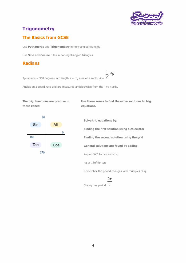
Trigonometry

The Basics from GCSE

Use Pythagoras and Trigonometry in right-angled triangles

Use Sine and Cosine rules in non-right-angled triangles

Radians

2p radians = 360 degrees, arc length s = rq, area of a sector A =

Angles on a coordinate grid are measured anticlockwise from the +ve x-axis.

The trig. functions are positive in

these zones:

Use these zones to find the extra solutions to trig.

equations.

Solve trig equations by:

1. Finding the first solution using a calculator

2. Finding the second solution using the grid

General solutions are found by adding:

2np or 3600 for sin and cos.

np or 1800 for tan

Remember the period changes with multiples of q.

Cos cq has period

5

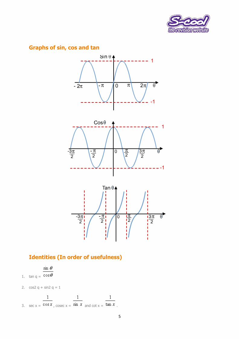
Graphs of sin, cos and tan

Identities (In order of usefulness)

1. tan q =

2. cos2 q + sin2 q = 1

3. sec x = , cosec x = and cot x = .

6

Double Angle Formulae

1. sin 2A = 2sin A cos A,

2. cos 2A = cos2 A - sin2 A = 1 - 2sin2 A = 2cos2 A - 1

3.

These came from the compound angle formulae:

1. sin (A + B) = sin A cos B + cos A sin B

2. sin (A - B) = sin A cos B - cos A sin B

3. cos (A + B) = cos A cos B - sin A sin B

4. cos (A - B) = cos A cos B + sin A sin B

R cos (q - a) is used to add sine and cosine functions together.

(i.e. acosq + bsinq = R cos (q - a)) and R and a are found by:

1. Expand the bracket

2. Match the question to the expansion

3. Find R and a using R = , and a =

Sometimes you may need the factor formulae (adding sines or cosines together) or the half-angle formulae

when integrating.

7

Basic Algebra

Basic Skills

Expanding 1 and 2 brackets (Practice)

Factorising a common factor into 1 bracket

Factorising a quadratic into 2 brackets

Solving Linear Equations

Solving Simultaneous Equations

Quadratics

Solve a quadratic equation by:

1. Rewriting the equation in the form ax2 + bx +c = 0.

2. Factorise.

3. Make each bracket = 0 to solve the equation

Alternatively: you can use the quadratic formula after step 1.

Completing the square

1. Rewrite in the form x2 + bx +c = 0, (if necessary divide by the multiple of x2)

2. Rewrite the x2 + bx as (x - b/2)2 -(b/2)2 so that x2 + bx +c = (x - b/2)2 -(b/2)2 + c

This gives you the minimum value of a quadratic: minimum value is the constant

(-(b/2)2 + c), when x = b/2.

If you know the roots of an equation then the original quadratic was:

x2 - (sum of roots) x + product of roots

Inequalities

Solve linear inequalities like normal equations. Remember (multiplying by -1) or (taking reciprocals) reverses the

inequality sign.

8

For quadratic inequalities: Solve the equation = 0, and then use the shape of the graph to finalise the

answer.

Remainder Theorem:

When dividing f(x) by (x - a), the remainder is f(a).

Factor Theorem:

If f(a) = 0, then (x - a) is a factor of f(x)

(When factorising polynomials, choose numbers that multiply together to make the constant.)

9

Advanced Algebra

Indices

Basic rules to learn are:

When using surds remember that:

Logarithms

Definition:

Logarithm Rules:

1.

2.

3.

An exponential equation is in the form: = value, and is solved by taking logs.

Binomial Expansion

To expand where n is a positive integer :

1. Write down a in descending powers - (from n to 0)

2. Write down b in ascending powers - (from 0 to n)

3. Add Binomial Coefficients from Pascals triangle, or by using: .

To expand , where n is not a positive integer:

10

1. Rearrange to get

2. Use the general formula

Remember the condition

Partial Fractions

These are used to turn complex expressions into simple fractions, which can then be used to integrate the

expression, or use the binomial expansion to get an approximation to the original expression.

Choose the appropriate formula from these:

1.

2.

3.

Then add the separate fractions together and match the numerators. You will need to use simultaneous

equations.

11

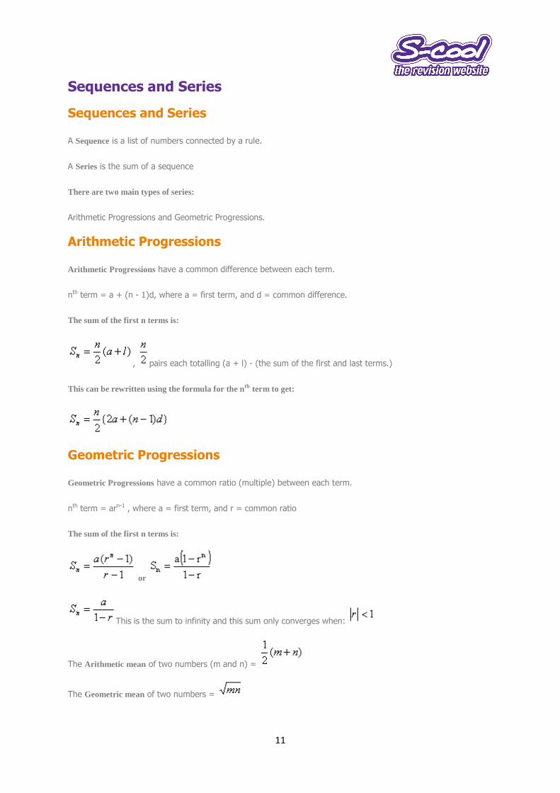
Sequences and Series

Sequences and Series

A Sequence is a list of numbers connected by a rule.

A Series is the sum of a sequence

There are two main types of series:

Arithmetic Progressions and Geometric Progressions.

Arithmetic Progressions

Arithmetic Progressions have a common difference between each term.

nth term = a + (n - 1)d, where a = first term, and d = common difference.

The sum of the first n terms is:

, pairs each totalling (a + l) - (the sum of the first and last terms.)

This can be rewritten using the formula for the nth term to get:

Geometric Progressions

Geometric Progressions have a common ratio (multiple) between each term.

nth term = arn-1 , where a = first term, and r = common ratio

The sum of the first n terms is:

or

This is the sum to infinity and this sum only converges when:

The Arithmetic mean of two numbers (m and n) =

The Geometric mean of two numbers =

12

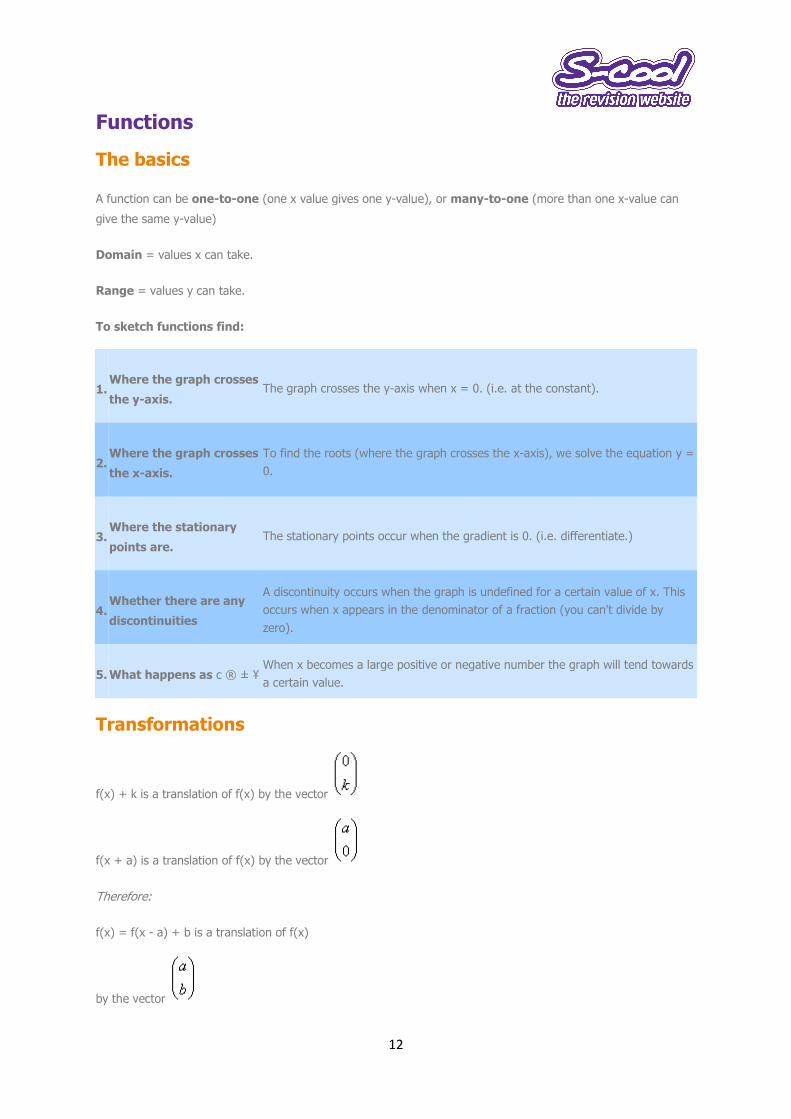
Functions

The basics

A function can be one-to-one (one x value gives one y-value), or many-to-one (more than one x-value can

give the same y-value)

Domain = values x can take.

Range = values y can take.

To sketch functions find:

1. Where the graph crosses

the y-axis. The graph crosses the y-axis when x = 0. (i.e. at the constant).

2. Where the graph crosses

the x-axis.

To find the roots (where the graph crosses the x-axis), we solve the equation y =

0.

3. Where the stationary

points are. The stationary points occur when the gradient is 0. (i.e. differentiate.)

4. Whether there are any

discontinuities

A discontinuity occurs when the graph is undefined for a certain value of x. This

occurs when x appears in the denominator of a fraction (you can't divide by

zero).

5. What happens as c ® ± ¥ When x becomes a large positive or negative number the graph will tend towards

a certain value.

Transformations

f(x) + k is a translation of f(x) by the vector

f(x + a) is a translation of f(x) by the vector

Therefore:

f(x) = f(x - a) + b is a translation of f(x)

by the vector

13

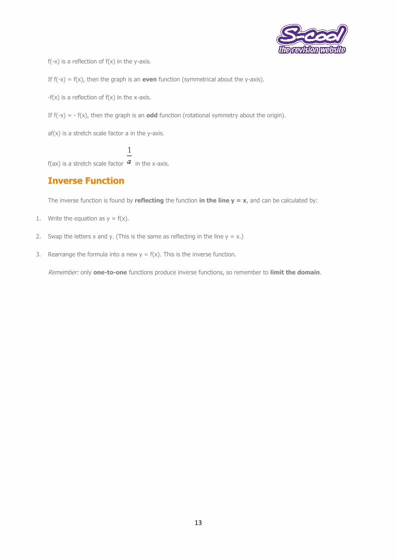
f(-x) is a reflection of f(x) in the y-axis.

If f(-x) = f(x), then the graph is an even function (symmetrical about the y-axis).

-f(x) is a reflection of f(x) in the x-axis.

If f(-x) = - f(x), then the graph is an odd function (rotational symmetry about the origin).

af(x) is a stretch scale factor a in the y-axis.

f(ax) is a stretch scale factor in the x-axis.

Inverse Function

The inverse function is found by reflecting the function in the line y = x, and can be calculated by:

1. Write the equation as y = f(x).

2. Swap the letters x and y. (This is the same as reflecting in the line y = x.)

3. Rearrange the formula into a new y = f(x). This is the inverse function.

Remember: only one-to-one functions produce inverse functions, so remember to limit the domain.

14

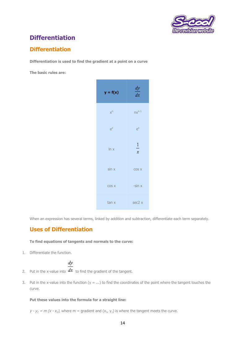
Differentiation

Differentiation

Differentiation is used to find the gradient at a point on a curve

The basic rules are:

y = f(x)

xn nxn-1

ex ex

ln x

sin x cos x

cos x -sin x

tan x sec2 x

When an expression has several terms, linked by addition and subtraction, differentiate each term separately.

Uses of Differentiation

To find equations of tangents and normals to the curve:

1. Differentiate the function.

2. Put in the x-value into to find the gradient of the tangent.

3. Put in the x-value into the function (y = ...) to find the coordinates of the point where the tangent touches the

curve.

Put these values into the formula for a straight line:

y - y1 = m (x - x1), where m = gradient and (x1, y1) is where the tangent meets the curve.

15

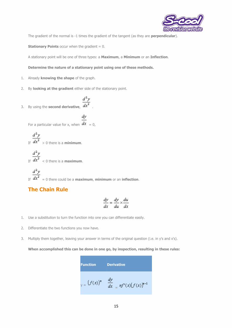
The gradient of the normal is -1 times the gradient of the tangent (as they are perpendicular).

Stationary Points occur when the gradient = 0.

A stationary point will be one of three types: a Maximum, a Minimum or an Inflection.

Determine the nature of a stationary point using one of these methods.

1. Already knowing the shape of the graph.

2. By looking at the gradient either side of the stationary point.

3. By using the second derivative, .

For a particular value for x, when = 0,

If > 0 there is a minimum.

If < 0 there is a maximum.

If = 0 there could be a maximum, minimum or an inflection.

The Chain Rule

1. Use a substitution to turn the function into one you can differentiate easily.

2. Differentiate the two functions you now have.

3. Multiply them together, leaving your answer in terms of the original question (i.e. in y's and x's).

When accomplished this can be done in one go, by inspection, resulting in these rules:

Function Derivative

y = =

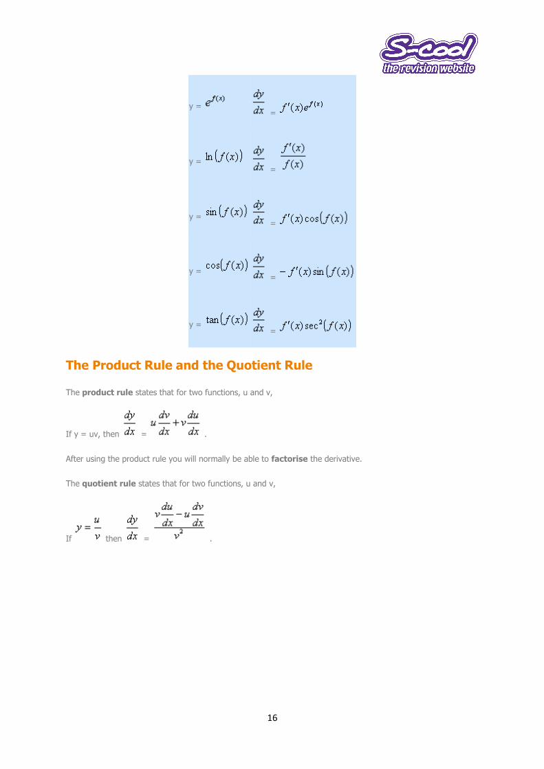
16

y = =

y = =

y = =

y = =

y = =

The Product Rule and the Quotient Rule

The product rule states that for two functions, u and v,

If y = uv, then = .

After using the product rule you will normally be able to factorise the derivative.

The quotient rule states that for two functions, u and v,

If then = .

17

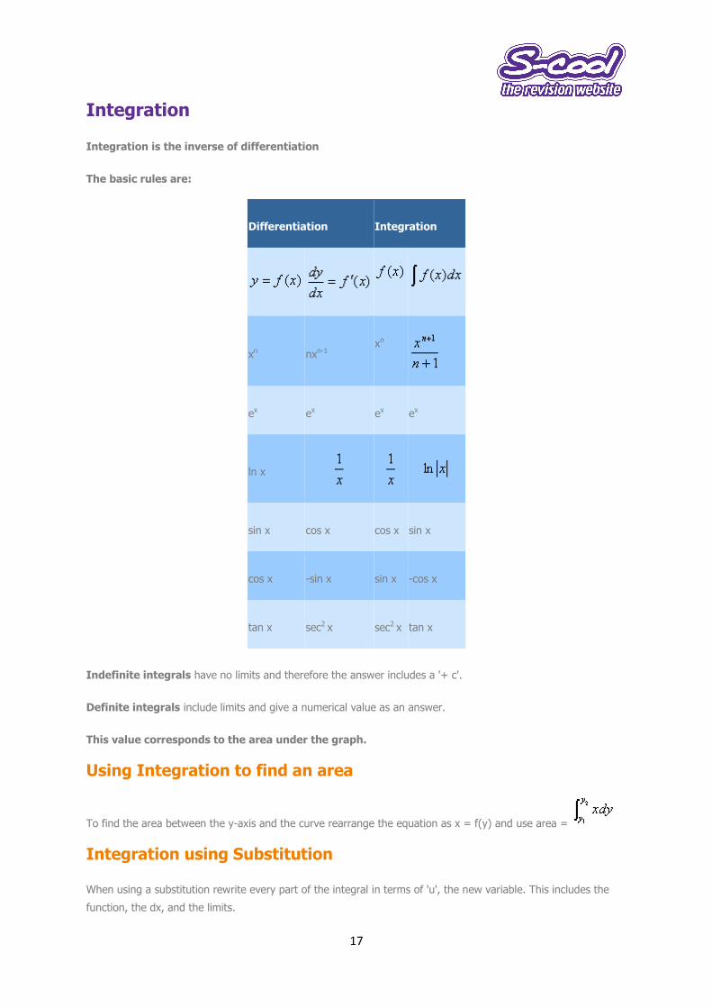
Integration

Integration is the inverse of differentiation

The basic rules are:

Differentiation Integration

xn nxn-1 xn

ex ex ex ex

ln x

sin x cos x cos x sin x

cos x -sin x sin x -cos x

tan x sec2 x sec2 x tan x

Indefinite integrals have no limits and therefore the answer includes a '+ c'.

Definite integrals include limits and give a numerical value as an answer.

This value corresponds to the area under the graph.

Using Integration to find an area

To find the area between the y-axis and the curve rearrange the equation as x = f(y) and use area =

Integration using Substitution

When using a substitution rewrite every part of the integral in terms of 'u', the new variable. This includes the

function, the dx, and the limits.

18

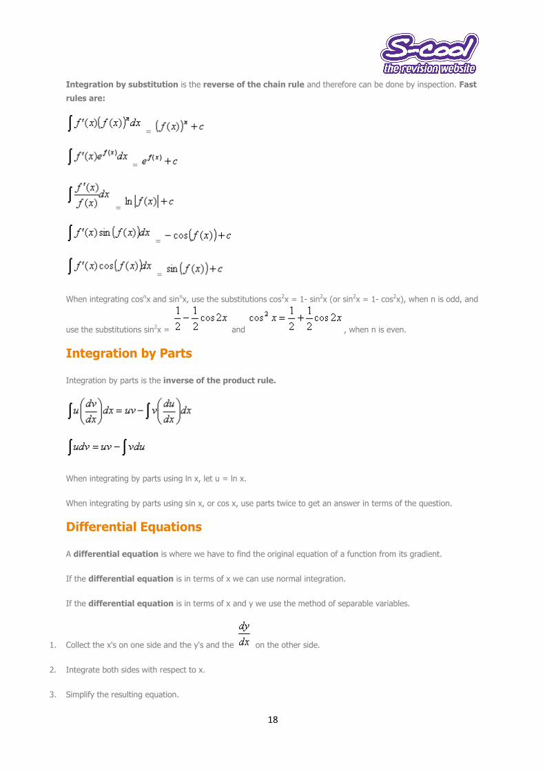
Integration by substitution is the reverse of the chain rule and therefore can be done by inspection. Fast

rules are:

=

=

=

=

=

When integrating cosnx and sinnx, use the substitutions cos2x = 1- sin2x (or sin2x = 1- cos2x), when n is odd, and

use the substitutions sin2x = and , when n is even.

Integration by Parts

Integration by parts is the inverse of the product rule.

When integrating by parts using ln x, let u = ln x.

When integrating by parts using sin x, or cos x, use parts twice to get an answer in terms of the question.

Differential Equations

A differential equation is where we have to find the original equation of a function from its gradient.

If the differential equation is in terms of x we can use normal integration.

If the differential equation is in terms of x and y we use the method of separable variables.

1. Collect the x's on one side and the y's and the on the other side.

2. Integrate both sides with respect to x.

3. Simplify the resulting equation.

19

Solving a differential equation results in a general solution (with a '+ c'). An illustration of this is called

a family of curves.

If we know one point on the graph we can find the particular solution.

20

Numerical Methods

Numerical Methods are systems, or algorithms, for solving equations that cannot be solved using normal

techniques.

Change of Sign Methods

1. Rearrange the equation into the form f(x) = 0

2. Sketch the graph of this function (using a calculator or by plotting points.)

3. Find an x-value that has a positive value for f(x), and an x-value that has a negative value for f(x).

4. (If the line is continuous) the roots of the equation will be between these two values of x.

We will not be able to find the root exactly, but we will be able to 'home in' on the root until we have it to the

desired degree of accuracy.

Interval Bisection

This allows you to get a more accurate solution to an equation than just using the Change of Sign Methods

alone.

1. Find values x that change the sign (as above).

2. Change one of the values to the average value of the two x values (i.e. )

3. Repeat step 2 above (each repetition is called an iteration), until you get solution that is accurate (i.e. correct

to 3 decimal places).

Linear Interpolation

Linear Interpolation is very similar to interval bisection; instead of taking the average of the two points

(i.e. ), it estimates that the root is on a straight line between the two points.

Steps to solve an equation are exactly as the Interval Bisection method (shown above), but replace the

equation with

The Newton Raphson method does not need a change of sign, but instead uses the tangent to the graph at a

known point to provide a better estimate for the root of the equation. It works on the basis that an estimate for

the root is found using the iteration:

21

.

Steps to find a solution:

1. Rearrange the equation to the format =0 and differentiate this to give .

2. Select an estimate of the root (i.e. the solution to the equation)

3. Put this estimate into the Newton Raphson equation

4. Perform step 3 until you get a consistent solution.

Rearrangement

1. Rearrange the equation to be solved into the form x = g(x).

2. The solution to this equation is to find where y = x meets y = g(x). This is where the coordinates on g(x) are the

same.

3. Guess a value xo and hope that g(xo) will be a better guess.

4. Take this solution and re-input it into the above step, until you get a consistent solution.

The solution may converge and provide you the solution OR it may diverge. In this case a solution will not be

found.

22

Vectors, Lines and Planes

1. Use Pythagoras to find the magnitude (length) of a vector.

2. The direction of a vector is the angle measured anti-clockwise from the +ve x-axis.

3. A position vector is the vector from the origin to a point.

4. Given the magnitude (r) and direction (q) of a vector, the coordinates of a point are (r cosq, r sinq).

5. Parallel vectors are multiples of each other.

6. Perpendicular vectors have a scalar product of 0.

7. Angles between vectors are found using:

Straight lines

A vector equation for a line is r = a + lb.

r = a general point on the line, a = a known point on the line, b = the direction of the line.

The Cartesian form is found by writing the x, y and z coordinates in terms of l.

Two lines intersect when their coordinates match. Find values of l and m that make all the coordinates match. If

two lines do not meet then they are skew.

The angle between two lines = angle between their direction vectors.

Planes

The vector equation of a plane is:

, where a is a vector to the plane, and b and c are vectors in the plane.

The Cartesian equation of a plane is found using:

r.n = a.n, where a is a point in the plane and n is the normal to the plane.

To find where a line meets a plane:

1. Write down the coordinates of a general point on the line.

2. Use these coordinates in the equation of the plane.

3. Solve the resulting equation and then find the coordinates.

To find the distance that a point is from a plane:

23

1. Use the normal of the plane to make the equation of the line joining the point to the corresponding point on the

plane.

2. Find where this line meets the plane.

3. Find the vector joining these two points.

4. Use Pythagoras to find the length of this vector.

The shortest distance from the origin to a plane is found by dividing the constant in the cartesian equation by the

length of the normal vector. (i.e. using the unit normal vector).

The angle between two planes is the same as the angle between the normals to the planes.

The angle between a line and a plane is 90o - angle between line and normal. Alternatively use:

where a = direction of the line, and n = normal vector.

24

The Basics

Data

There are 2 types of data:

1. Qualitative - where the data is not numerical.

2. Quantitative - where the data is numerical.

Quantitative data is the most useful set of data to us and can be in 2 forms:

1. Discrete data - can only take certain values.

2. Continuous data - this set of data can take any value within a given range.

Note: measuring will give us continuous data whereas counting will give discrete.

Averages

The mode is the most popular value or values, i.e. the piece or pieces of data that occur most often.

The median is the middle piece of data when the data is in numerical order.

In general, to find the place of the median of n pieces of data we can use the following 2 rules:

1. n odd - then use ½(n + 1) (the value just over halfway).

2. n even - we find halfway between ½n and the next value (halfway and the next value).

The mean of a set of data is the sum of all the values divided by the number of values.

The mean is denoted by and for n pieces of data is calculated by:

just means the sum of all the x's - for instance, add all the bits of data together.

Quartiles

The lower quartile is the value 25% (1/4) of the way through the distribution.

The upper quartile is the value 75% (3/4) of the way through the distribution.

The median is the value 50% (1/2) of the way through the distribution.

Standard deviation

The standard deviation gives a measure of how the data is dispersed about the mean, the centre of the data.

There are 2 formulae for calculating the standard deviation, .

25

Formula 1 =

Formula 2 =

The variance is the square of the standard deviation.

Variance =

26

Representation of Data

Stem-and-leaf and box-and-whisker diagrams

A stem-and-leaf diagram is one way of taking raw data and presenting it in an easy and quick way to

help spot patterns in the spread of the data. They are best used when we have a relatively small set

of data and want to find the median or quartiles.

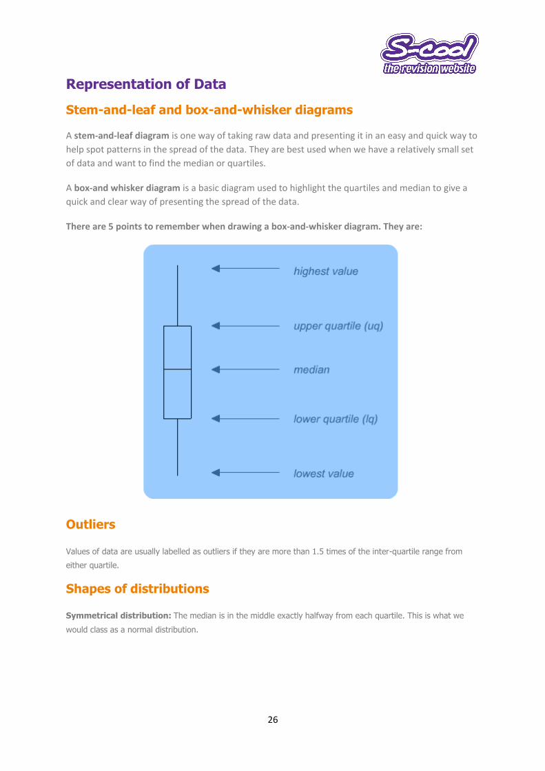
A box-and whisker diagram is a basic diagram used to highlight the quartiles and median to give a

quick and clear way of presenting the spread of the data.

There are 5 points to remember when drawing a box-and-whisker diagram. They are:

Outliers

Values of data are usually labelled as outliers if they are more than 1.5 times of the inter-quartile range from

either quartile.

Shapes of distributions

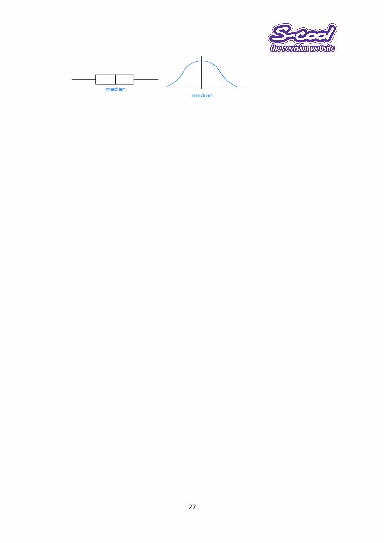
Symmetrical distribution: The median is in the middle exactly halfway from each quartile. This is what we

would class as a normal distribution.

27

28

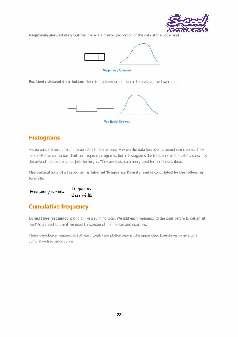
Negatively skewed distribution: there is a greater proportion of the data at the upper end.

Positively skewed distribution: there is a greater proportion of the data at the lower end.

Histograms

Histograms are best used for large sets of data, especially when the data has been grouped into classes. They

look a little similar to bar charts or frequency diagrams, but in histograms the frequency of the data is shown by

the area of the bars and not just the height. They are most commonly used for continuous data.

The vertical axis of a histogram is labelled 'Frequency Density' and is calculated by the following

formula:

Cumulative frequency

Cumulative frequency is kind of like a running total. We add each frequency to the ones before to get an 'at

least' total. Best to use if we need knowledge of the median and quartiles.

These cumulative frequencies ('at least' totals) are plotted against the upper class boundaries to give us a

cumulative frequency curve.

29

Probability

Permutations

The number of permutations of arranging n distinct (different) objects is:

n! (n factorial)

n! = n x (n - 1) x (n - 2) x ... x 2 x 1

The number of ways of arranging n objects of which r are the same is:

In addition to this the number of ways of arranging n objects of p of one type are alike, q of a second type are

alike, r of a third type are alike etc.

This is given by:

The number of permutations of r objects from n is written as npr.

We write:

Handy hint: Nearly all permutation questions involve putting things in order from a line where the order matters.

For example, ABC is a different permutation to ACB.

Combinations

Suppose that we wish to choose r objects from n, but the order in which the objects are arranged does not

matter. Such a choice is called a combination. ABC would be the same combination as ACB as they include all the

same letters.

The number of combinations of r objects from n, distinct, objects can be written in 2 ways:

Probability

The probability that an event, A, will happen is written as P(A).

The probability that the event A, does not happen is called the complement of A and is written as A'

30

As either A must or must not happen then,

P(A') = 1 - P(A) as probability of a certainty is equal to 1.

Set notation

If A and B are two events then:

A B represents the event 'both A and B occur'

A B represents the event 'either A or B occur'

Mutually Exclusive Events

Two events are mutually exclusive if the event of one happening excludes the other from happening. In other

words, they both cannot happen simultaneously.

For exclusive events A and B then:

P(A or B) = P(A) + P(B) this can be written in set notation as

P(A B) = P(A) + P(B)

This can be extended for three or more exclusive events

P(A or B or C) = P(A) + P(B) + P(C)

Handy hint: Exclusive events will involve the words 'or', 'either' or something which implies 'or'. Remember 'OR'

means 'add'.

Independent Events

Two events are independent if the occurrence of one happening does not affect the occurrence of the other.

For independent events A and B then: P(A and B) = P(A) + P(B)

This can be written in set notation as: P(A B) = P(A) + P(B)

Again, this result can be extended for three or more events: P(A and B and C) = P(A) + P(B) + P(C)

Handy hint: Independent events will involve the words 'and', 'both' or something which implies either of these.

Remember 'and' means 'multiply'.

Tree diagrams

Most problems will involve a combination of exclusive and independent events. One of the best ways to answer

these questions is to draw a tree diagram to cover all the arrangements.

31

The Addition Law

If two events, A and B, are not mutually exclusive then the probability that A or B will occur is given by the

addition formula: P(A B) = P(A) + P(B) - P(A B)

The probability of A or B occurring is the probability of A add the probability of B minus the probability that they

both occur.

Conditional Probability

If we need to find the probability of an event occurring given that another event has already occurred then we

are dealing with Conditional probability.

If A and B are two events then the conditional probability that A occurs given that B already has is written

as where:

Or:

If we rearrange this formula we obtain another useful result:

If the two events A and B are independent (for instance, one doesn't affect the other), then quite

clearly,

32

Probability Distributions

Discrete random variable

A random variable is a variable which takes numerical values and whose value depends on the outcome of an

experiment. It is discrete if it can only take certain values.

For a discrete random variable X with P(X = x) then probabilities always sum to 1.

P(X = x) = 1 (Remember means 'sum of').

Cumulative distribution function

'Cumulative' gives us a kind of running total, so a cumulative distribution function gives us a running total of

probabilities within our probability table.

The cumulative distribution function, F(x) of X is defined as:

Expectation

The expectation is the expected value of X, written as E(X) or sometimes as .

The expectation is what you would expect to get if you were to carry out the experiment a large number of times

and calculate the 'mean'.

To calculate the expectation we can use: E(X) = x P(X = x)

Expectation of any function of x

If X is a discrete random variable and f(x) is any function of x, then the expected value of f(x) is given by: E[f(x)]

= f(x)P(X = x)

There are a few general results we should remember to help with our calculations of expectations: E(a) = a

E(aX + b) = aE(X) + b

Variance

The variance is a measure of how spread out the values of X would be if the experiment leading to X were

repeated a number of times.

The variance of X, written as Var(X) is given by:

Var(X) = E(X2) - (E(X))2, If we write E(X) = then,

Var(X) = E(X2) - 2

Or Var(X) = E(X - )2, this tells us that Var(X) 0

33

There are a few general results we should remember to help with our calculations of variances:

Var(aX) = a2Var(X)

Var(aX + b) = a2Var(X)

The Standard Deviation

The square root of the Variance is called the Standard Deviation of X. Standard deviation is given the symbol .

= or Var(X) = 2

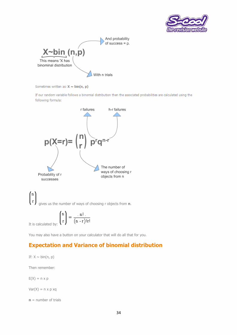
The Binomial Distribution

Suppose that an experiment consists of n identical and independent trials, where for each trial there are 2

outcomes.

'Success' which is given probability p

'Failure' which is given probability q where q = 1 - p

Then if X = the number of successes, we say that X has a binomial distribution. We write:

34

gives us the number of ways of choosing r objects from n.

It is calculated by:

You may also have a button on your calculator that will do all that for you.

Expectation and Variance of binomial distribution

If: X ~ bin(n, p)

Then remember:

E(X) = n x p

Var(X) = n x p xq

n = number of trials

35

p = probability of a success

q = probability of a failure = 1 - p

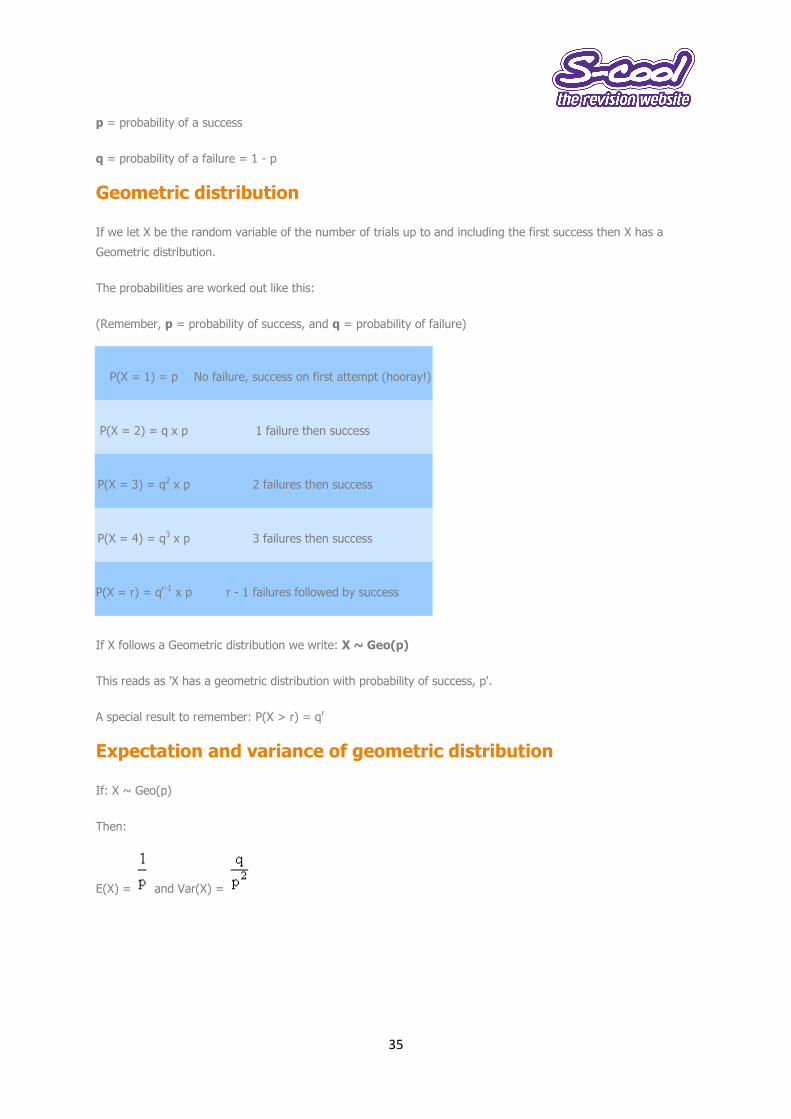
Geometric distribution

If we let X be the random variable of the number of trials up to and including the first success then X has a

Geometric distribution.

The probabilities are worked out like this:

(Remember, p = probability of success, and q = probability of failure)

P(X = 1) = p No failure, success on first attempt (hooray!)

P(X = 2) = q x p 1 failure then success

P(X = 3) = q2 x p 2 failures then success

P(X = 4) = q3 x p 3 failures then success

P(X = r) = qr-1 x p r - 1 failures followed by success

If X follows a Geometric distribution we write: X ~ Geo(p)

This reads as 'X has a geometric distribution with probability of success, p'.

A special result to remember: P(X > r) = qr

Expectation and variance of geometric distribution

If: X ~ Geo(p)

Then:

E(X) = and Var(X) =

36

The Normal Distribution

Many naturally occurring phenomena can be approximated using a continuous random variable

called The Normal Distribution. For example; the height of females or the weight of Russian ballet

dancers.

In a normal distribution, much of the data is gathered around the mean. The distribution has a

characteristic 'bell shape' symmetrical about the mean.

Remember we write the symbol, , to stand for the mean. The area of the bell shape = 1.

In any normal distribution, approximately 68% of the data will lie within one standard deviation of

the mean. The standard deviation is an important measure of the spread of our data. The greater

the standard deviation, the greater our spread of data.

We write the symbol, , to stand for the standard deviation. The standard deviation squared gives us the

variance: Var(X) = 2

The Normal Distribution tables

If X has a normal distribution with mean, , and variance, 2, then we write: X ~ N( , 2)

37

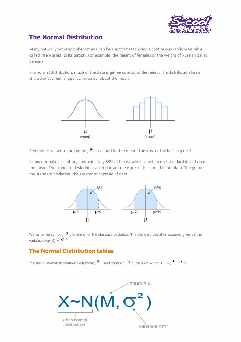
We will look closely at the normal distribution Z, with mean, = 0, and variance = 1.

Z ~ N(0, 1)

Suppose for this distribution we wanted to calculate the P(Z < 1). Unlike with our discrete random variables we

don't have a formula to work this out (there is one but it's way beyond the scope of A-Level maths!). The values

of these probabilities have already been calculated and are tabulated in most statistics books.

With Z ~ N(0, 1) the P(Z = z) = (z)

Don't be put off with the Greek letter (phi). (z) just describes the area under the bell from that point!

Normal distribution and standardising

X ~ N( , 2) and standardising

The only values of the normal distribution that are tabulated are from Z ~ N(0, 1). Not many distributions will

have a mean of 0 and a variance of 1 however, so we need to convert any normal distribution of X into the

normal distribution of Z!

This is done using the formula: Z = X -

Where is the mean and is the standard deviation.

38

Bivariate Data

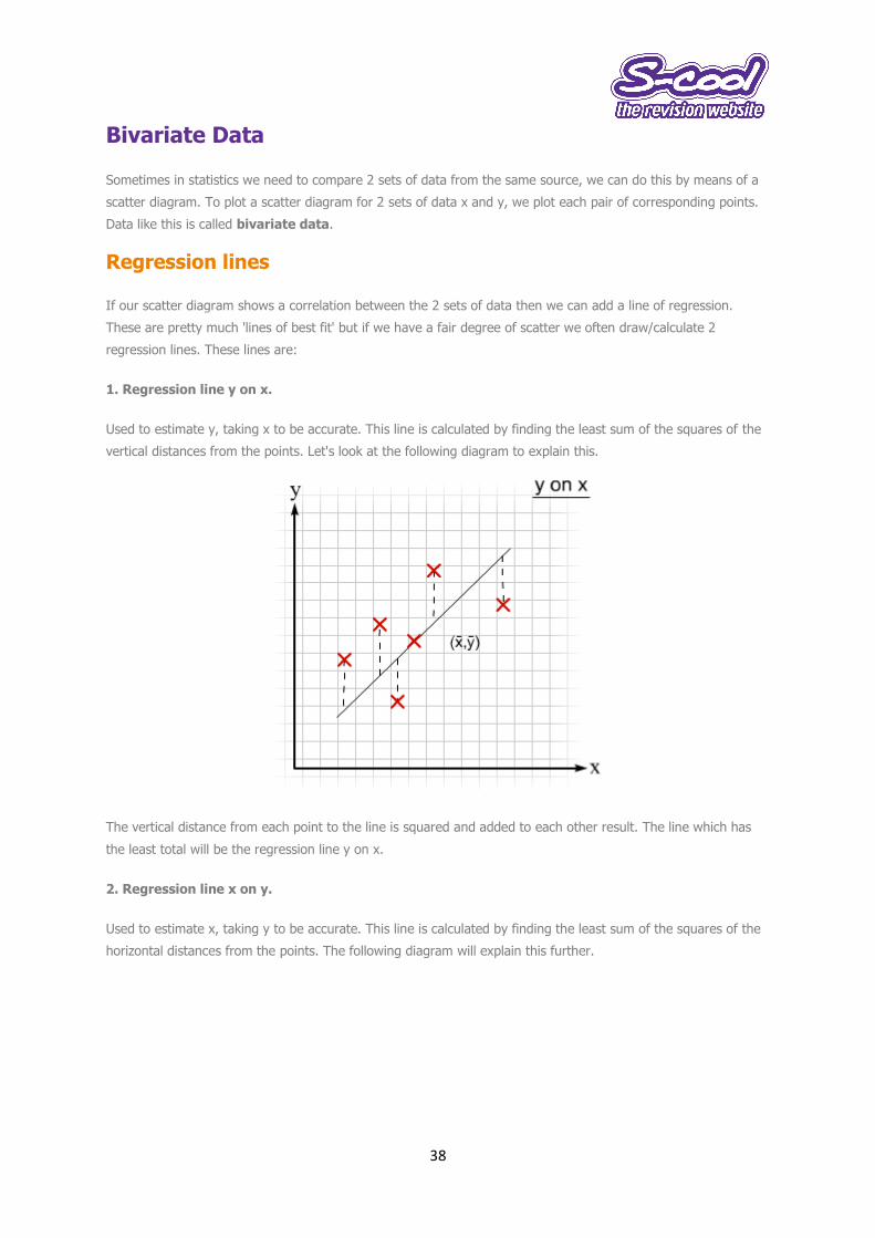
Sometimes in statistics we need to compare 2 sets of data from the same source, we can do this by means of a

scatter diagram. To plot a scatter diagram for 2 sets of data x and y, we plot each pair of corresponding points.

Data like this is called bivariate data.

Regression lines

If our scatter diagram shows a correlation between the 2 sets of data then we can add a line of regression.

These are pretty much 'lines of best fit' but if we have a fair degree of scatter we often draw/calculate 2

regression lines. These lines are:

1. Regression line y on x.

Used to estimate y, taking x to be accurate. This line is calculated by finding the least sum of the squares of the

vertical distances from the points. Let's look at the following diagram to explain this.

The vertical distance from each point to the line is squared and added to each other result. The line which has

the least total will be the regression line y on x.

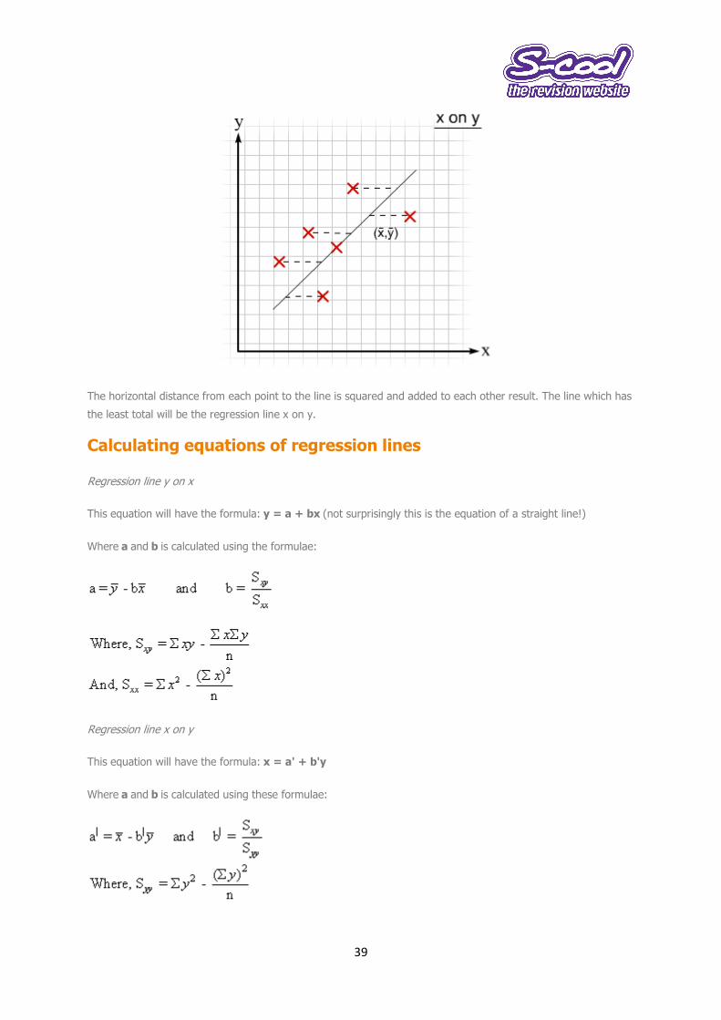
2. Regression line x on y.

Used to estimate x, taking y to be accurate. This line is calculated by finding the least sum of the squares of the

horizontal distances from the points. The following diagram will explain this further.

39

The horizontal distance from each point to the line is squared and added to each other result. The line which has

the least total will be the regression line x on y.

Calculating equations of regression lines

Regression line y on x

This equation will have the formula: y = a + bx (not surprisingly this is the equation of a straight line!)

Where a and b is calculated using the formulae:

Regression line x on y

This equation will have the formula: x = a' + b'y

Where a and b is calculated using these formulae:

40

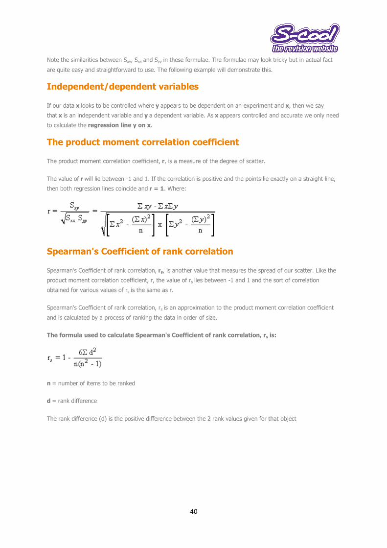
Note the similarities between Sxy, Sxx and Syy in these formulae. The formulae may look tricky but in actual fact

are quite easy and straightforward to use. The following example will demonstrate this.

Independent/dependent variables

If our data x looks to be controlled where y appears to be dependent on an experiment and x, then we say

that x is an independent variable and y a dependent variable. As x appears controlled and accurate we only need

to calculate the regression line y on x.

The product moment correlation coefficient

The product moment correlation coefficient, r, is a measure of the degree of scatter.

The value of r will lie between -1 and 1. If the correlation is positive and the points lie exactly on a straight line,

then both regression lines coincide and r = 1. Where:

Spearman's Coefficient of rank correlation

Spearman's Coefficient of rank correlation, rs, is another value that measures the spread of our scatter. Like the

product moment correlation coefficient, r, the value of rs lies between -1 and 1 and the sort of correlation

obtained for various values of rs is the same as r.

Spearman's Coefficient of rank correlation, rs is an approximation to the product moment correlation coefficient

and is calculated by a process of ranking the data in order of size.

The formula used to calculate Spearman's Coefficient of rank correlation, rs is:

n = number of items to be ranked

d = rank difference

The rank difference (d) is the positive difference between the 2 rank values given for that object

41

Terms and conditions

All S-cool content (including these notes) belong to S-cool (S-cool Youth Marketing Limited).

You may use these for your personal use on a computer screen, print pages on paper and store such pages in

electronic form on disk (but not on any server or other storage device connected to an external network) for

your own personal, educational, non-commercial purposes.

You may not redistribute any of this Content or supply it to other people (including by using it as part of any

library, archive, intranet or similar service), remove the copyright or trade mark notice from any copies or

modify, reproduce or in any way commercially exploit any of the Content.

All copyright and publishing rights are owned by S-cool. First created in 2000 and updated in 2013.