A Lattice Boltzmann Method

applied to the heat equation

Stephane DELLACHERIE∗ and Christophe LE POTIER

CEA-Saclay, France

Dec. 5, 2008

∗Contacts: stephane.dellacherie@cea.fr and (+33)1.69.08.98.11

0-0

Outlines:

1 - Introduction

2 - Fluid limit of a simple kinetic system

3 - Two LBM schemes

4 - Links with a finite-difference type scheme

5 - Some properties: convergence and maximum principle

6 - Numerical results

7 - Two strange properties

8 - Conclusion

1

1 - Introduction

The LBM method is said to be :

1) simple and explicit;

2) unconditionally stable and accurate;

3) adapted to model porous medium;

4) parallelisable.

Nevertheless, the LBM method is not really known in the applied

math. community.

WHY ?

2

In fact, the LBM scheme is often presented ...

• Point 1) ... as a physical model that is more general than the

EDPs it is supposed to solve. For example:

“It is known that existence-uniqueness-regularity problems are very

hard at the Navier-Stokes level (...). However,

at the lattice Boltzmann level, [there is] no existence, uniqueness

and regularity problems.” In : U. Frisch, Phycica D, 47, p. 231-232, 1991.

Or: “It may appear unusual that (...) in the LBM approach,

the approximation of the flow equation is only shown

after the method is already postulated.”

In : Mishra et al, Journal of Heat and Mass Transfer, 48, p. 3648-3659, 2005.

As a consequence, the LBM scheme is often described with:

LBM scheme → continuous EDPs

(as it is the case for the Boltzmann equation) instead of

continuous EDPs → discretization → LBM scheme.

3

• Point 2) ... as a miraculous numerical method:

Example : “ (...) the Lattice Boltzmann technique may be

regarded as a new [explicit] finite-difference technique for the

Navier-Stokes equation

having the property of unconditionnal stability.” (Mishra et al.).

The aim of this talk is to give precise math. justifications of all

these assertions in the simple case of the heat equation.

4

We propose the following approach:

continuous kinetic system ⇐⇒ continuous heat eq.

(ε = “collision time”) ε ≪ 1 (fluid limit when ε ≪ 1)

↓ l

↓ links with finite differences ?

discretization with ε ≪ 1 stability, convergence in L∞ ?

↓ ↑

LBM scheme → discretization of

the heat eq. since ε ≪ 1 ?

We can summerize this approach (which is the standard approach in num. anal.) with:

Continuous EDP → discretization → LBM scheme → stability, convergence ?

instead of:

LBM scheme as a “physical” model → discretization → continuous EDP

5

2 - Fluid limit of a simple kinetic system

Construction of a simple kinetic system:

We firstly define the “maxwellian” distribution

Mq :=ρ

2

[1 +

u(x)

vq

]=

ρ

2

[1 + (−1)q u(x)

c

](vq = (−1)qc)

where u(x) is a given function and c ∈ R+. It verifies

∑

q=1,2

1

vq

Mq =

ρ

ρu

.

6

Proposition 1 Let fq(t, x) be solution of the kinetic system

∂tfq + (−1)qc∂xfq =1

ε(Mq − fq) (q = 1, 2) (1)

where Mq := f1+f2

2

[1 + (−1)q u(x)

c

]. Thus, the density ρ := f1 + f2

is solution up to the order ε2 of

∂tρ + ∂x(uρ) = ν∂2xxρ with ν = εc2 (2)

when |u(x)| ≪ c and ε ≪ 1. Moreover, we have

fq(t, x) =ρ

2

[

1 + (−1)q u(x)

c+ ε(−1)q

(du2

dx(x)

2c− c

∂xρ

ρ

)]

+ O(ε2).

Proof : We use an Hilbert or Chapman-Enskog expansion.�

7

When u = 0 :

Corollary 1 Let fq(t, x) be solution of the kinetic system

∂tfq + (−1)qc∂xfq =1

ε(Mq − fq) (q = 1, 2) (3)

with Mq := f1+f2

2 . Thus, the density ρ := f1 + f2 is solution up to

the order ε2 of

∂tρ = ν∂2xxρ with ν = εc2 (4)

when ε ≪ 1. Moreover, we have

fq(t, x) =ρ

2

[1 + (−1)q+1cε

∂xρ

ρ

]+ O(ε2).

Let us note that ε ≪ 1 means ε ≪ tfluid where tfluid = O(1).

8

3 - Construction of two LBM schemes

3.1 - Integration of the kinetic system

Proposition 2 Let {fq(t, x)}q=1,2 be solution of

∂tfq + (−1)qc∂xfq =1

ε(Mq − fq) := Qq(f)(t, x) (q = 1, 2)

and let

gq(t, x) := fq(t, x) − ∆t2 Qq(f)(t, x).

Thus

gq[t+∆t, x+(−1)qc∆t] = gq(t, x)(1−η)+Mq(t, x)η+ O(∆t3

ε) (5)

where

η =1

ε∆t

+ 12

.

Since g1 + g2 = f1 + f2 := ρ, it is possible to propose a LBM scheme by using the

discrete version of (5) i.e. by using the variable gnq,i instead of fn

q,i.

9

Proof of the proposition 2:

The solution of the continuous EDP

∂tfq + (−1)qc∂xfq =1

ε(Mq − fq) := Qq(f)(t, x)

is given by

fq[t+∆t, x+(−1)qc∆t] = fq(t, x)+

∫ ∆t

0

Qq(f)[t+s, x+(−1)qcs]ds.

A classical numerical integration would give

fq [t + ∆t, x + (−1)qc∆t] = fq(t, x) + ∆tQq(f)(t, x) + O(∆t2

ε).

But O(∆t2

ε) = O(∆t) (since ε = O(∆t): see the sequel ...).

Thus, we use the integration formula

fq[t + ∆t, x + (−1)qc∆t] = fq(t, x) + ∆t2 [Qq(f)(t, x)

+ Qq(f)(t + ∆t, x + (−1)qc∆t)]

+ O(∆t3

ε).

10

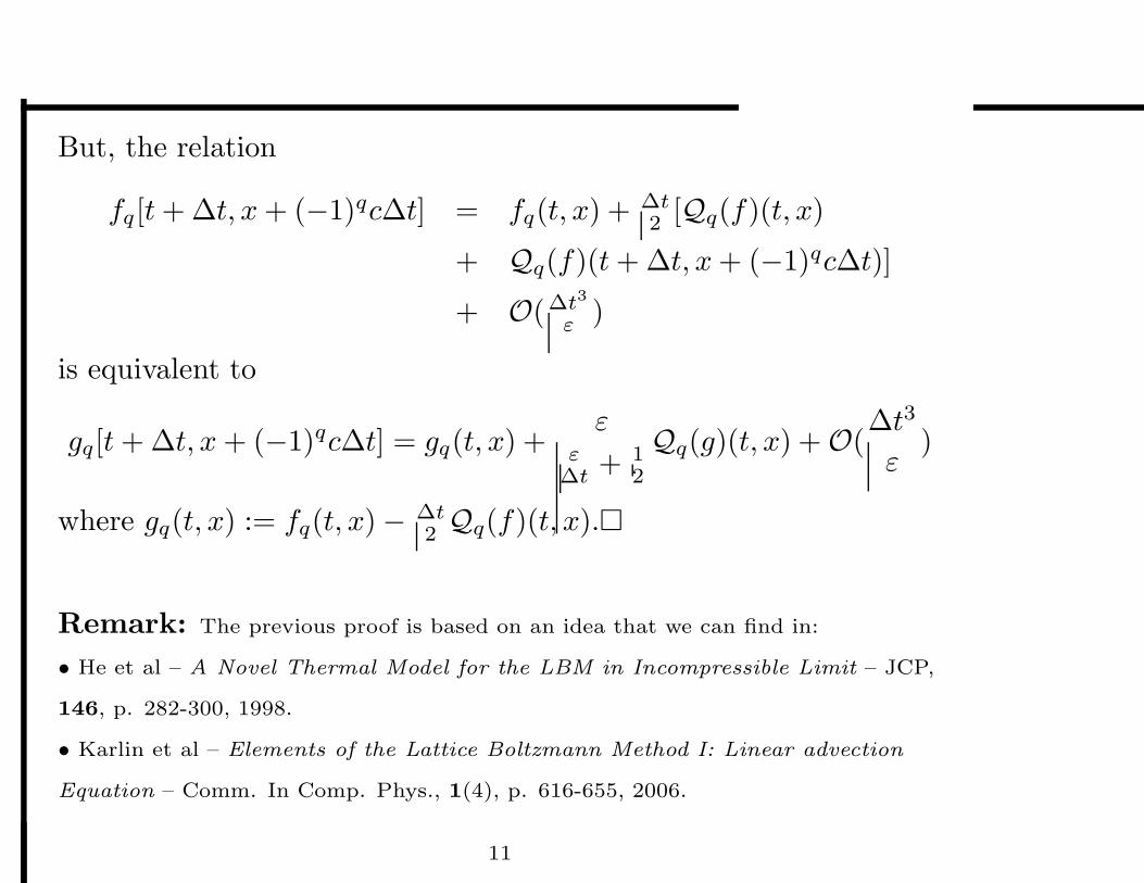
But, the relation

fq[t + ∆t, x + (−1)qc∆t] = fq(t, x) + ∆t2 [Qq(f)(t, x)

+ Qq(f)(t + ∆t, x + (−1)qc∆t)]

+ O(∆t3

ε)

is equivalent to

gq[t + ∆t, x + (−1)qc∆t] = gq(t, x) +ε

ε∆t

+ 12

Qq(g)(t, x) + O(∆t3

ε)

where gq(t, x) := fq(t, x) − ∆t2 Qq(f)(t, x).�

Remark: The previous proof is based on an idea that we can find in:

• He et al – A Novel Thermal Model for the LBM in Incompressible Limit – JCP,

146, p. 282-300, 1998.

• Karlin et al – Elements of the Lattice Boltzmann Method I: Linear advection

Equation – Comm. In Comp. Phys., 1(4), p. 616-655, 2006.

11

3.2 - A first LBM scheme

We choose:

c = ∆x

∆t,

ε = νc2

=⇒ ε = Cd∆t with ∆t := Cd

∆x2

ν> 0

(Cd > 0). We deduce from the estimate (cf. proposition 2)

gq[t + ∆t, x + (−1)qc∆t] = gq(t, x)(1 − η) + Mq(t, x)η + O(∆t3

ε)

(where η = 1ε

∆t+ 1

2

) a first LBM scheme:

gn+11,i = gn

1,i+1(1 − η) + Mn1,i+1η,

gn+12,i = gn

2,i−1(1 − η) + Mn2,i−1η,

ρn+1i = gn+1

1,i + gn+12,i

whereη = 1

Cd+ 12

= 1ν∆t

∆x2 + 12

.

12

By noting that Mq = g1+g2

2 , we see that the LBM scheme is

equivalent to

gn+11,i = gn

1,i+1(1 − η2 ) + gn

2,i+1η2 ,

gn+12,i = gn

2,i−1(1 − η2 ) + gn

2,i−1η2 ,

ρn+1i = gn+1

1,i + gn+12,i

whereη = 1

Cd+ 12

= 1ν∆t

∆x2 + 12

.

We will use this formulation in the sequel.

Let us remark that η ∈]0, 2[ when Cd (i.e. ∆t) ∈ R+∗ .

13

The “magic” formula: It is possible to writte the previous LBM scheme

with

gn+11,i = gn

1,i+1(1 − ∆tbε ) + Mn

1,i+1∆tbε ,

gn+12,i = gn

2,i−1(1 − ∆tbε ) + Mn

2,i−1∆tbε ,

ρn+1i = gn+1

1,i + gn+12,i

where ε is such that ν =(ε − ∆t

2

) (∆x∆t

)2.

To simplify the situation, most of the LBM schemes are written with

∆x = ∆t = 1 and without the function g:

f1(t + 1, x − 1) = f1(t, x)(1 − 1

bε ) + M1(t, x) 1bε ,

f2(t + 1, x + 1) = f2(t, x)(1 − 1bε ) + M2(t, x) 1

bε

where ν =(ε − 1

2

)c2s with cs := “sound velocity”(= 1 here).

For example: D. Wolf-Gladrow – A Lattice Bolzmann Equation for Diffusion – J.

of Stat. Phys., 79(5,6), p. 1023-1032, 1995.

14

A last remark:

By noting that

gq(t, x) := fq(t, x) −∆t

2Qq(f)(t, x),

we can rewrite the LBM scheme

gn+11,i = gn

1,i+1(1 − η2 ) + gn

2,i+1η2 ,

gn+12,i = gn

2,i−1(1 − η2 ) + gn

2,i−1η2

whereη = 1

Cd+ 12

= 1ν∆t

∆x2 + 12

.

with the fq variable. We obtain the LBM scheme:

fn+11,i =

fn1,i+1(16C2

d−1)+fn2,i+1(4Cd+1)+fn

2,i−1(4Cd−1)+fn1,i−1

16Cd(Cd+ 12 )

,

fn+12,i =

fn1,i+1(4Cd−1)+fn

2,i+1+fn2,i−1(16C2

d−1)+fn1,i−1(4Cd+1)

16Cd(Cd+ 12 )

.

15

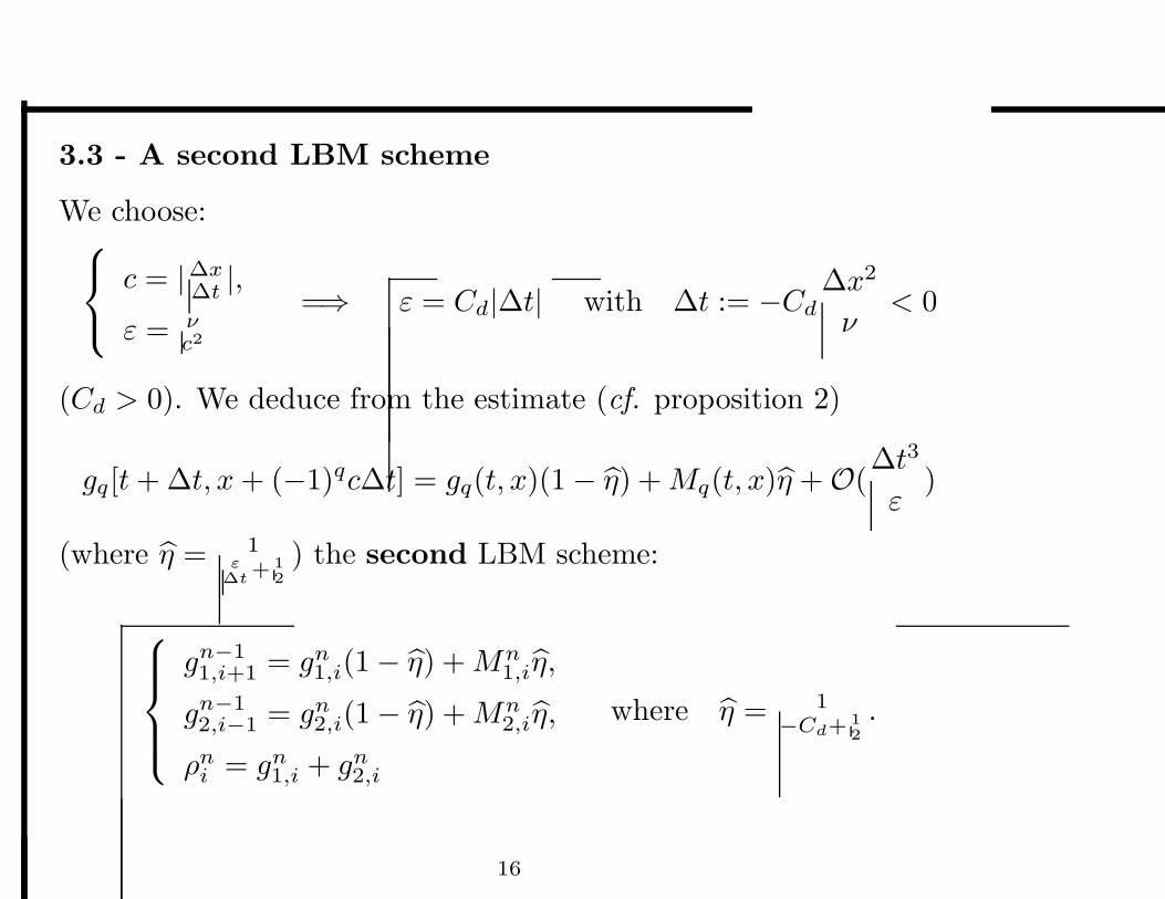
3.3 - A second LBM scheme

We choose:

c = |∆x

∆t|,

ε = νc2

=⇒ ε = Cd|∆t| with ∆t := −Cd

∆x2

ν< 0

(Cd > 0). We deduce from the estimate (cf. proposition 2)

gq[t + ∆t, x + (−1)qc∆t] = gq(t, x)(1 − η) + Mq(t, x)η + O(∆t3

ε)

(where η = 1ε

∆t+ 1

2

) the second LBM scheme:

gn−11,i+1 = gn

1,i(1 − η) + Mn1,iη,

gn−12,i−1 = gn

2,i(1 − η) + Mn2,iη,

ρni = gn

1,i + gn2,i

where η = 1−Cd+ 1

2

.

16

We have the property:

Property 1 The LBM scheme

gn−11,i+1 = gn

1,i(1 − η) + Mn1,iη,

gn−12,i−1 = gn

2,i(1 − η) + Mn2,iη,

ρni = gn

1,i + gn2,i

where η =1

−Cd + 12

is equivalent to the LBM scheme

gn+11,i = gn

1,i+1(1 − η2 ) + gn

2,i−1η2 ,

gn+12,i = gn

2,i−1(1 − η2 ) + gn

1,i+1η2 ,

ρn+1i = gn+1

1,i + gn+12,i

where η =1

Cd + 12

with ∆t := Cd∆x2

ν. We name this scheme LBM∗ scheme.

17

QUESTIONS:

• LBM = LBM∗ ?

• initial conditions gn=01,i and gn=0

2,i ?

• boundary conditions ?

• stability and convergence ?

• probabilistic interpretation (not treated in this talk) ?

18

4 - Links with a finite-difference type scheme

Les us recall the two LBM schemes:

• LBM scheme:

gn+11,i = gn

1,i+1(1 − η2 ) + gn

2,i+1η2 ,

gn+12,i = gn

2,i−1(1 − η2 ) + gn

1,i−1η2 ,

ρn+1i = gn+1

1,i + gn+12,i

whereη = 1

Cd+ 12

= 1ν∆t

∆x2 + 12

.

• LBM∗ scheme:

gn+11,i = gn

1,i+1(1 − η2 ) + gn

2,i−1η2 ,

gn+12,i = gn

2,i−1(1 − η2 ) + gn

1,i+1η2 ,

ρn+1i = gn+1

1,i + gn+12,i

whereη = 1

Cd+ 12

= 1ν∆t

∆x2 + 12

.

Here, we only study the LBM∗ scheme which is more simple to

study than the LBM scheme. Nevertheless, all the properties

verified by the LBM∗ scheme are also verified by the LBM scheme.

19

Dirichlet boundary conditions

ρ(t, xmin) = ρxminand xi = xmin + i∆x (i = 1, . . .).

Lemma 1 The LBM∗ scheme with the boundary condition

gn+12,i=0 = ρxmin − gn

1,i=1 + η(gn1,i=1 −

12ρxmin),

g02,i=0 = αρxmin

(n ∈ {0, . . .})

and with the initial condition

{g01,i = (1 − α)ρ0

i ,

g02,i = αρ0

i

(i ∈ {1, . . .})

is equivalent to the Du Fort-Frankel scheme

ρn+1i −ρ

n−1i

2∆t= ν

∆x2 (ρni+1 − ρn+1

i − ρn−1i + ρn

i−1),

ρn0 = ρxmin

(6)

when ρn=1i in (6) is defined with

ρn=1i := αρ0

i−1 + (1 − α)ρ0i+1.

20

Remarks:

• We have a similar result for Neumann B.C. when

gn+12,i=0 = gn+1

1,i=1 + (gn2,i=0 − gn

1,i=1)(1 − η),

g02,i=0 = αρ0

i=1

(n ∈ {0, . . .})

and we recover the bounce-back B.C. gn2,i=0 = gn

1,i=1

when α = 1/2.

• This equivalence between a LBM scheme and a finite-difference

scheme was firstly mentioned in:

Ancona M.G. – Fully-Lagrangian and Lattice-Boltzmann Methods for Solving

Systems of Conservation Equations – JCP, 115, p. 107-120, 1994.

Nevertheless, the importance of the initial and boundary

conditions was not studied.

• the Robin B.C. has not been studied.

21

5 - Some properties: convergence and maximum principle

5.1 - Convergence in L∞

Proposition 3 For any Cd > 0 (∆t := Cd∆x2

ν) and any α ∈ R:

i) the LBM∗ schemes with periodic, Neumann or Dirichlet B.C.

and with the initial condition

g01,i = (1 − α)ρ0

i ,

g02,i = αρ0

i

(i ∈ {1, . . .})

converge in L∞;

ii) the Du Fort-Frankel scheme

ρn+1i − ρn−1

i

2∆t=

ν

∆x2(ρn

i+1 − ρn+1i − ρn−1

i + ρni−1)

with periodic, Neumann or Dirichlet B.C. converges in L∞ when

ρn=1i := αρ0

i−1 + (1 − α)ρ0i+1;

iii) the convergence order is equal to 2 ⇐⇒ α = 12 .

22

Basic idea of the proof:

unconditional L∞ stability of the LBM∗ scheme [due to convexity]

+ equivalence lemma (i.e. lemma 1)

⇓

unconditional L∞ stability of the Du Fort-Frankel scheme

AND

Lax theorem (stability + consistency)

⇓

unconditional L∞ convergence of the Du Fort-Frankel scheme

AND

equivalence lemma (i.e. lemma 1)

⇓

unconditional L∞ convergence of the LBM∗ schemes.

23

Some comments: Recall that ∆t := Cd∆x2

ν.

• It is known since 1953 that the Du Fort-Frankel scheme is

unconditionally stable in L2 under periodic B.C. (cf. Fourier

analysis).

• But, since the Du Fort-Frankel scheme may be written with

(1 + 2ν∆t

∆x2)ρn+1

i = (1 − 2ν∆t

∆x2)ρn−1

i + 2ν∆t

∆x2(ρn

i+1 + ρni−1),

we have also the L∞ stab. under the stab. cond. 0 ≤ Cd ≤ 1/2

(since the maximum principle is verified in that case).

• Here, we have obtained the unconditional L∞ stability of the Du

Fort-Frankel scheme when

ρn=1i := αρ0

i−1 + (1 − α)ρ0i+1, α ∈ R.

24

5.2 - Maximum principle with periodic and Neumann B.C.

Lemma 2 For any Cd ≥ 0 (∆t := Cd∆x2

ν), the LBM∗ scheme with

the initial condition

g01,i = (1 − α)ρ0

i ,

g02,i = αρ0

i

(i ∈ {1, . . .})

verifies the maximum principle

minj

ρ0j ≤ ρn

i ≤ maxj

ρ0j

i) for any α ∈ [0, 1] in the periodic case;

ii) when α = 12 in the Neumann case.

Thus, this is also the case for the Du Fort-Frankel scheme with periodic or

Neumann B.C. when the first iterate is defined with ρn=1i := αρ0

i−1 + (1 − α)ρ0i+1.

Remark: for the periodic B.C. (cf. point i), the result is also valid for the LBM sch.. Nevertheless,

for the Neumann B.C. (cf. point ii), the result has still to be proved for the LBM scheme.

25

Remark:

The Du Fort-Frankel scheme is equivalent to

ρn+1i = ρn

i+1(1 −η

2) + ρn

i−1(1 −η

2) + ρn−1

i (η − 1)

(with η := 1ν∆t

∆x2 + 12

∈ [0, 2]). Thus, when ρn=1i := αρ0

i−1 + (1 − α)ρ0i+1:

ρ2i = [αρ0

i + (1 − α)ρ0i+2](1 − η

2 )

+[αρ0i−2 + (1 − α)ρ0

i ](1 − η2 ) + ρ0

i (η − 1)

= [αρ0i−2 + (1 − α)ρ0

i+2](1 − η2 ) + ρ0

iη2 .

This proves that: minj

ρ0j ≤ ρ2

i ≤ maxj

ρ0j for any ∆t > 0

for the periodic case when α ∈ [0, 1].

Nevertheless, it is a priori more difficult to obtain a similar result

for ρn≥3i without using the LBM equivalence !!!

26

5.3 - Maximum principle with modified Dirichlet B.C.

In the Dirichlet case

gn+12,i=0 = ρxmin − gn

1,i=1 + η(gn1,i=1 −

12ρxmin),

g02,i=0 = αρxmin

(7)

(idem in x = xmax), the maximum principle

min(ρxmin , ρxmax , minj

ρ0j ) ≤ ρn

i ≤ max(ρxmin , ρxmax , maxj

ρ0j)

is verified when 0 ≤ Cd ≤ 12 .

We would like this maximum principle to be unconditionally

satisfied (as for the periodic and Neumann cases),

to be able to treat the case Cd > 12 and cells number = O(1).

→ We have to modify the Dirichlet B.C. (7).

→ We will lose the equivalence LBM / Du Fort-Frankel !!!

27

Lemma 3 For any Cd ≥ 0 (∆t := Cd∆x2

ν), the LBM∗ scheme with

the modified Dirichlet boundary condition

gn2,i=0 = 1

2ρxmin ,

gn1,i=N+1 = 1

2ρxmax

(8)

and with the initial condition

g01,i = g0

2,i =ρ0

i

2

verifies the maximum principle

min(ρxmin , ρxmax , minj

ρ0j ) ≤ ρn

i ≤ max(ρxmin , ρxmax , maxj

ρ0j).

Some comments: With the modified Dirichlet B.C. (8) →8>>>><>>>>:

i) loss of the equivalence LBM - Du Fort-Frankel;

ii) convergence ?

iii) a priori, loss of the order 2 (verified with numerical experiments);

iv) but ROBUST on ROUGH mesh because of the maximum principle !!!

28

6 - Numerical results

We test the LBM∗ scheme

gn+11,i = gn

1,i+1(1 − η2 ) + gn

2,i−1η2 ,

gn+12,i = gn

2,i−1(1 − η2 ) + gn

1,i+1η2 ,

ρn+1i = gn+1

1,i + gn+12,i

where

η =1

Cd + 12

=1

ν∆t∆x2 + 1

2

.

We choose [xmin, xmax] = [−10, 10] and ν = 1.

29

Test-case 1: Maximum principle with order 2 or (order 1 ?) modified

Dirichlet B.C.

We study the influence of the order 2 Dirichlet B.C.

gn+12,i=0 = ρxmin − gn

1,i=1 + η(gn1,i=1 −

12ρxmin),

g02,i=0 = 1

2ρxmin

and of the (order 1 ?) modified Dirichlet B.C.

gn2,i=0 = 1

2ρxmin ,

gn1,i=N+1 = 1

2ρxmax

on the maximum principle when the mesh is ROUGH

(we think that this is an important test for porous medium).

Here, cells number = 10 and the initial condition is given by

ρ0i = 1

4 if i 6∈ {5, 6}

= 34 if i ∈ {5, 6}.

We choose Cd = 4 and tfinal = tn=10.

30

ρn=4i with order 2 Dirichlet B.C. (Cd = 4)

−10 −8 −6 −4 −2 0 2 4 6 8 100.2

0.3

0.4

0.5

0.6

0.7

0.8

0.9

1.0

1.1

1.2

−10 −8 −6 −4 −2 0 2 4 6 8 10−0.1

0.0

0.1

0.2

0.3

0.4

0.5

0.6

0.7

0.8

ρxmin = ρxmax = 1 ρxmin = ρxmax = 0

ρn=4i with (order 1 ?) modified Dirichlet B.C. (Cd = 4)

−10 −8 −6 −4 −2 0 2 4 6 8 100.2

0.3

0.4

0.5

0.6

0.7

0.8

0.9

1.0

−10 −8 −6 −4 −2 0 2 4 6 8 100.0

0.1

0.2

0.3

0.4

0.5

0.6

0.7

0.8

ρxmin = ρxmax = 1 ρxmin = ρxmax = 0

30-1

Test-case 2: instat. analyt. sol. with order 2 or (order 1 ?)

modified Dirichlet B.C. and with a fine mesh

We compare the results with the analytical solution

φ(t, x) = erf

[xi − xmin√4ν(t + t0)

]

(with t0 = 1).

We impose the order 2 or (order 1 ?) modified Dirichlet B.C. with

ρn

xmin= φ(tn, xmin),

ρnxmax

= φ(tn, xmax).

We choose cells number = 100, Cd ∈ {2, 4, 8, 16} and tfinal = 15.

31

Order 2 Dirichlet B.C.ρn

i and ρexact(tn, xi) (tn = 15)

−10 −8 −6 −4 −2 0 2 4 6 8 100.0

0.1

0.2

0.3

0.4

0.5

0.6

0.7

0.8

0.9

1.0

−10 −8 −6 −4 −2 0 2 4 6 8 100.0

0.1

0.2

0.3

0.4

0.5

0.6

0.7

0.8

0.9

1.0

Cd = 2 Cd = 4

−10 −8 −6 −4 −2 0 2 4 6 8 100.0

0.1

0.2

0.3

0.4

0.5

0.6

0.7

0.8

0.9

1.0

−10 −8 −6 −4 −2 0 2 4 6 8 100.0

0.1

0.2

0.3

0.4

0.5

0.6

0.7

0.8

0.9

1.0

Cd = 8 Cd = 16

31-1

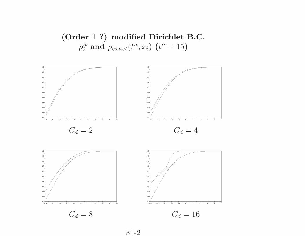
(Order 1 ?) modified Dirichlet B.C.ρn

i and ρexact(tn, xi) (tn = 15)

−10 −8 −6 −4 −2 0 2 4 6 8 100.0

0.1

0.2

0.3

0.4

0.5

0.6

0.7

0.8

0.9

1.0

−10 −8 −6 −4 −2 0 2 4 6 8 100.0

0.1

0.2

0.3

0.4

0.5

0.6

0.7

0.8

0.9

1.0

Cd = 2 Cd = 4

−10 −8 −6 −4 −2 0 2 4 6 8 100.0

0.1

0.2

0.3

0.4

0.5

0.6

0.7

0.8

0.9

1.0

−10 −8 −6 −4 −2 0 2 4 6 8 100.0

0.1

0.2

0.3

0.4

0.5

0.6

0.7

0.8

0.9

1.0

Cd = 8 Cd = 16

31-2

Convergence (LBM∗ scheme)

Erreur L2(∆x) (—) et y = x1 ou 2 (- - -)

pour N ∈ {50, 100, 500} (Cd = 2)

1e-04

0.001

0.01

0.1

1

0.01 0.1 1 0.001

0.01

0.1

1

0.01 0.1 1

Order 2 Dirichlet B.C. (Order 1 ?) modified Dirichlet B.C.

Thus, the modified Dirichlet B.C. seems to be of order 1. This B.C. is

adapted when the mesh is rough (cf. porous medium) since the max. principle is

verified (ROBUST code). But, when the mesh is fine, the order 2 is better.

32

Test-case 3: Influence of the first iterate ρn=1i on the

properties of the Du Fort-Frankel scheme

We impose periodic boundary condition.

We choose cells number = 100 and Cd = 4.

We choose the initial condition

ρ0i = 0 si i 6= 50

= 1 si i = 50

(i.e. ρ0i = Dirac in x = 0).

33

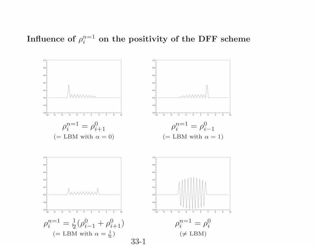
Influence of ρn=1i on the positivity of the DFF scheme

−10 −8 −6 −4 −2 0 2 4 6 8 10−0.4

−0.2

0.0

0.2

0.4

0.6

0.8

1.0

−10 −8 −6 −4 −2 0 2 4 6 8 10−0.4

−0.2

0.0

0.2

0.4

0.6

0.8

1.0

ρn=1i = ρ0

i+1 ρn=1i = ρ0

i−1

(= LBM with α = 0) (= LBM with α = 1)

−10 −8 −6 −4 −2 0 2 4 6 8 10−0.4

−0.2

0.0

0.2

0.4

0.6

0.8

1.0

−10 −8 −6 −4 −2 0 2 4 6 8 10−0.4

−0.2

0.0

0.2

0.4

0.6

0.8

1.0

ρn=1i = 1

2 (ρ0i−1 + ρ0

i+1) ρn=1i = ρ0

i

(= LBM with α = 12 ) ( 6= LBM)

33-1

7 - Two strange properties

(∆t = Cd∆x2

ν)

• Cd = 0 :

Lemma 4 When Cd = 0 (i.e. ∆t = 0), the LBM∗ scheme

preserves the initial condition in the sense

Cd = 0 =⇒ ∀n ∈ N : ρni = ρn+2

i .

Thus, the Du Fort-Frankel scheme verifies the same property when

the first iterate is defined with ρn=1i := αρ0

i−1 + (1 − α)ρ0i+1.

• Cd = +∞ :

When Cd → +∞, we observe waves and discontinuities !!!

34

Dirichlet B.C. and Cd = 1000

−10 −8 −6 −4 −2 0 2 4 6 8 100.0

0.1

0.2

0.3

0.4

0.5

0.6

0.7

0.8

0.9

1.0

−10 −8 −6 −4 −2 0 2 4 6 8 100.0

0.1

0.2

0.3

0.4

0.5

0.6

0.7

0.8

0.9

1.0

tn=10 tn=20

−10 −8 −6 −4 −2 0 2 4 6 8 100.0

0.1

0.2

0.3

0.4

0.5

0.6

0.7

0.8

0.9

1.0

−10 −8 −6 −4 −2 0 2 4 6 8 100.0

0.1

0.2

0.3

0.4

0.5

0.6

0.7

0.8

0.9

1.0

tn=30 tn=40

34-1

Neumann B.C. and Cd = 1000

−10 −8 −6 −4 −2 0 2 4 6 8 100.0

0.1

0.2

0.3

0.4

0.5

0.6

0.7

0.8

0.9

1.0

−10 −8 −6 −4 −2 0 2 4 6 8 100.0

0.1

0.2

0.3

0.4

0.5

0.6

0.7

0.8

0.9

1.0

tn=10 tn=20

−10 −8 −6 −4 −2 0 2 4 6 8 100.0

0.1

0.2

0.3

0.4

0.5

0.6

0.7

0.8

0.9

1.0

−10 −8 −6 −4 −2 0 2 4 6 8 100.0

0.1

0.2

0.3

0.4

0.5

0.6

0.7

0.8

0.9

1.0

tn=40 tn=80

34-2

We can explain this phenomena:

When Cd → +∞ (i.e. ∆t → +∞), the LBM and LBM∗ is given by

gn+11,i = gn

1,i+1,

gn+12,i = gn

2,i−1,

ρn+1i = gn+1

1,i + gn+12,i .

The distributions gq are advected with the velocity vq = (−1)q ∆x∆t

.

Thus, ρni cannot converge toward the stationary solution of the heat

equation when ∆t → +∞.

35

More precisely, we can prove that the consistency error E of the

Dufort-Frankel scheme is given by E = −ν ∆t2

∆x2 ∂2ttρ + O(∆x2).

Thus, the equivalent equation is given by

∂tρ = ν(∂2xxρ − 1

c2 ∂2ttρ) + O(∆x2) with c =

∆x

∆t

(telegraph equation).

→ This means that the Du Fort-Frankel scheme is consistent

under the consistency condition ∆t = Cd∆x2

ν.

Thus, when Cd → +∞ or when ∆t = Cst∆x, the LBM scheme

solves the wave equation

∂2ttρ − c2∂2

xxρ = 0 with c =∆x

∆t.

This explains why there are waves and discontinuities

when Cd → +∞.

36

Thus: although the LBM scheme is unconditionally stable,

we do not have to choose a large Cd.

More precisely, the LBM scheme is consistent

under the condition ∆t = Cst∆xα (α > 1).

But, from a practical point of view, how to choose Cd ?

It depends on the test-case and on the mesh.

37

9 - Conclusion

• construction of two LBM schemes for ∂tρ = ν∂2xxρ;

• equivalence with a particular class of Du Fort-Frankel schemes for

periodic, Neumann and Dirichlet B.C.;

• convergence of this particular class of Du Fort-Frankel schemes in

L∞ for any ∆t := Cd∆x2

ν∈ R

+;

• maximum principle for any ∆t ∈ R+ with periodic and order 2

Neumann B.C., but not with the order 2 Dirichlet B.C.;

• modification of the order 2 Dirichlet B.C. → LBM scheme with a

order 1 Dirichlet B.C.;

=⇒ maximum principle for any ∆t ∈ R+ for the LBM scheme with

this new order 1 Dirichlet B.C.;

• it is possible to propose a probabilistic interpretation of the LBM

scheme and of the Du Fort-Frankel scheme: could it be a general

tool to analyse LBM schemes for other equations ?

38