Embed Size (px)
Citation preview

A Language for Mathematical KnowledgeManagement
Steve Kieffer
September 2, 2007


Acknowledgements
This work would not have been possible without the patience and guidance of myadvisor Jeremy Avigad, or without ideas which came both from him and from HarveyFriedman.
I am also grateful for thoughtful comments and revisions from Joe Ramsey.
Thanks also to my parents, who were indispensable in preparing and practicing a talkon this material.
It is dedicated to my brother Matt, who would have insisted this be published infanzine format if he were still with us today.


Contents
1 Introduction 1
2 LPT, the Language of Proofless Text 7
2.1 Syntax . . . . . . . . . . . . . . . . . . . . . . . . . . . . . . . . . . . 7
2.1.1 Terms and Formulas . . . . . . . . . . . . . . . . . . . . . . . 7
2.1.2 Definitions . . . . . . . . . . . . . . . . . . . . . . . . . . . . . 11
2.2 Special Features . . . . . . . . . . . . . . . . . . . . . . . . . . . . . . 13
2.3 Parsing . . . . . . . . . . . . . . . . . . . . . . . . . . . . . . . . . . . 17
3 First application: Translation 21
3.1 Formalization, translation, and reduction . . . . . . . . . . . . . . . . 22
3.2 A translation target system . . . . . . . . . . . . . . . . . . . . . . . 23
3.3 DZFC . . . . . . . . . . . . . . . . . . . . . . . . . . . . . . . . . . . 24
3.4 Conservativity . . . . . . . . . . . . . . . . . . . . . . . . . . . . . . . 27
3.4.1 The four systems . . . . . . . . . . . . . . . . . . . . . . . . . 27
3.4.2 The extension theorems . . . . . . . . . . . . . . . . . . . . . 31
3.4.3 Second extension . . . . . . . . . . . . . . . . . . . . . . . . . 38
3.4.4 Third extension . . . . . . . . . . . . . . . . . . . . . . . . . . 45
3.5 Sample input-output pairs . . . . . . . . . . . . . . . . . . . . . . . . 46
4 Second application: Structural observations 49
4.1 Dags . . . . . . . . . . . . . . . . . . . . . . . . . . . . . . . . . . . . 50
4.2 Quantifier depths . . . . . . . . . . . . . . . . . . . . . . . . . . . . . 52
4.2.1 Quantifier data . . . . . . . . . . . . . . . . . . . . . . . . . . 54
4.2.2 Calculating quantifier depths for expanded definitions . . . . . 55
4.3 Symbol counts . . . . . . . . . . . . . . . . . . . . . . . . . . . . . . . 57
4.4 Types . . . . . . . . . . . . . . . . . . . . . . . . . . . . . . . . . . . 57
v

vi CONTENTS
5 Third application: Knowledge graphs 595.1 kmap . . . . . . . . . . . . . . . . . . . . . . . . . . . . . . . . . . . . 595.2 Future directions . . . . . . . . . . . . . . . . . . . . . . . . . . . . . 62
A Characters and Strings in LPT 65A.1 Characters . . . . . . . . . . . . . . . . . . . . . . . . . . . . . . . . . 65A.2 Strings . . . . . . . . . . . . . . . . . . . . . . . . . . . . . . . . . . . 67
B Our LPT grammar is not LL 69B.1 Proof . . . . . . . . . . . . . . . . . . . . . . . . . . . . . . . . . . . . 69B.2 The grammar . . . . . . . . . . . . . . . . . . . . . . . . . . . . . . . 71
C DAG depth and size data 87C.1 Foundations – Suppes . . . . . . . . . . . . . . . . . . . . . . . . . . 87C.2 Topology – Munkres . . . . . . . . . . . . . . . . . . . . . . . . . . . 90
D Quantifier depth data 97D.1 Foundations – Suppes . . . . . . . . . . . . . . . . . . . . . . . . . . 97D.2 Topology – Munkres . . . . . . . . . . . . . . . . . . . . . . . . . . . 103
E Symbol count data 111E.1 Foundations – Suppes . . . . . . . . . . . . . . . . . . . . . . . . . . 111E.2 Topology – Munkres . . . . . . . . . . . . . . . . . . . . . . . . . . . 117
F Definitions: Foundations – Suppes 125F.1 Chapter 2 . . . . . . . . . . . . . . . . . . . . . . . . . . . . . . . . . 125F.2 Chapter 3 . . . . . . . . . . . . . . . . . . . . . . . . . . . . . . . . . 126F.3 Chapter 4 . . . . . . . . . . . . . . . . . . . . . . . . . . . . . . . . . 141F.4 Chapter 5 . . . . . . . . . . . . . . . . . . . . . . . . . . . . . . . . . 142F.5 Chapter 6 . . . . . . . . . . . . . . . . . . . . . . . . . . . . . . . . . 151
G Definitions: Topology – Munkres 175G.1 Section 12 . . . . . . . . . . . . . . . . . . . . . . . . . . . . . . . . . 175G.2 Section 13 . . . . . . . . . . . . . . . . . . . . . . . . . . . . . . . . . 177G.3 Section 14 . . . . . . . . . . . . . . . . . . . . . . . . . . . . . . . . . 181G.4 Section 15 . . . . . . . . . . . . . . . . . . . . . . . . . . . . . . . . . 185G.5 Section 16 . . . . . . . . . . . . . . . . . . . . . . . . . . . . . . . . . 186G.6 Section 17 . . . . . . . . . . . . . . . . . . . . . . . . . . . . . . . . . 188G.7 Section 18 . . . . . . . . . . . . . . . . . . . . . . . . . . . . . . . . . 191

CONTENTS vii
G.8 Section 19 . . . . . . . . . . . . . . . . . . . . . . . . . . . . . . . . . 193G.9 Section 20 . . . . . . . . . . . . . . . . . . . . . . . . . . . . . . . . . 196G.10 Section 21 . . . . . . . . . . . . . . . . . . . . . . . . . . . . . . . . . 201G.11 Section 22 . . . . . . . . . . . . . . . . . . . . . . . . . . . . . . . . . 202G.12 Section 23 . . . . . . . . . . . . . . . . . . . . . . . . . . . . . . . . . 204G.13 Section 24 . . . . . . . . . . . . . . . . . . . . . . . . . . . . . . . . . 205G.14 Section 25 . . . . . . . . . . . . . . . . . . . . . . . . . . . . . . . . . 208G.15 Section 26 . . . . . . . . . . . . . . . . . . . . . . . . . . . . . . . . . 212G.16 Section 27 . . . . . . . . . . . . . . . . . . . . . . . . . . . . . . . . . 213G.17 Section 28 . . . . . . . . . . . . . . . . . . . . . . . . . . . . . . . . . 215G.18 Section 29 . . . . . . . . . . . . . . . . . . . . . . . . . . . . . . . . . 216G.19 Section 30 . . . . . . . . . . . . . . . . . . . . . . . . . . . . . . . . . 217G.20 Section 31 . . . . . . . . . . . . . . . . . . . . . . . . . . . . . . . . . 219G.21 Section 32 . . . . . . . . . . . . . . . . . . . . . . . . . . . . . . . . . 220G.22 Section 33 . . . . . . . . . . . . . . . . . . . . . . . . . . . . . . . . . 221G.23 Section 34 . . . . . . . . . . . . . . . . . . . . . . . . . . . . . . . . . 222G.24 Section 35 . . . . . . . . . . . . . . . . . . . . . . . . . . . . . . . . . 223G.25 Section 36 . . . . . . . . . . . . . . . . . . . . . . . . . . . . . . . . . 224G.26 Section 37 . . . . . . . . . . . . . . . . . . . . . . . . . . . . . . . . . 227G.27 Section 38 . . . . . . . . . . . . . . . . . . . . . . . . . . . . . . . . . 227

viii CONTENTS

Chapter 1
Introduction
We live at a time at which, on the one hand, mathematical research is producing moreand more knowledge; and on the other hand the abilities of computers to managedata are becoming better and better understood. It is natural then that in the lastcouple of decades efforts have been launched in a field called Mathematical KnowledgeManagement (MKM), in which computer systems are being designed for a number ofpurposes pertaining to mathematical knowledge. The field is represented each yearat the conference on MKM which has met annually since 2002.
While the ‘management’ in the name of the field is perhaps most directly sug-gestive of database maintenance, the field is properly understood to include projectswith a wider variety of purposes than this. Others include the presentation and visu-alization of mathematical knowledge, interactive instruction in mathematics, and theformal verification of mathematical knowledge. This breadth of subjects is reflectedin the variety of papers collected each year in the MKM conference proceedings [4].
Meanwhile efforts are underway in the philosophy of mathematics to clarify thenature of, and differences between, such things as mathematical understanding, skill,and knowledge. (See [6] for example, and references cited therein.) While philoso-phers working in this area continue to clarify what it is that mathematical knowledgeconsists of, we may certainly for the time being take theorems, and defined conceptsto constitute at least part of it. We may therefore direct our present efforts in MKMtoward the design of systems to manage these two sorts of mathematical product. Inthis project, I focus on definitions.
In order to use computer systems to store, retrieve, manipulate, measure for com-plexity, or even depict, the content of mathematical definitions and theorems, andin order to computationally verify theorems, we need a suitable language in whichthe definitions and theorems can be written. The central contribution of the present
1
2 CHAPTER 1. INTRODUCTION
thesis project is the presentation of such a language, along with the development ofa computer system to parse input written in this language, and store it in a formamenable to further use.
As peripheral contributions I have designed three other computer systems servingMKM purposes, each of which utilizes the data stored by the first system. I discussthem in greater detail below. Briefly, they are (1) A translator, translating the inputlanguage to the language of a system of set theory; (2) Programs that gather variousstructural data from definitions; and (3) A graphical user interface allowing the userto explore the conceptual dependencies among defined concepts.
By way of testing the parser, I have compiled a database of 341 definitions, whichcan be found in Appendices F and G. These are formalized versions of the definitionsappearing in two textbooks: (1) Chapters 2 through 6 of Suppes’s Axiomatic SetTheory [15]; and (2) Sections 12 through 38 of Munkres’s Topology [12]. I did notformalize any theorems, as the definitions were enough to meet the goals of thisproject.
Likewise, the database was assembled just for the purposes of the immediateproject, and is not expected to be usable by others, at least not in its present form.This made it possible to bracket important database and search issues, for the timebeing.
In the future, however, we may have to consider such issues, for example, searcha-bility. Keyword search will certainly be possible, if we keep the database in its presentform. On the other hand, semantic search would be desirable too, and for this wewould benefit by augmenting the current definition syntax to allow for semantic tags,indicating subject matter.
A serious attempt to develop a definition library would also prompt better namingconventions. For one thing we might want to allow the database to be distributedacross servers, and in that case namespaces would be a good idea. Even if not, itwould be wise to set down rules for naming definitions in a way that reflects theirsources (as I have done in the definitions appearing in Appendices F and G).
Finally, we have also deferred questions as to whether the definitions in ourdatabase could be interchangeable with other MKM systems.
The input language considered in this project was designed by Harvey Friedman.With the view in mind that written mathematics consists of theorems, definitions,and proofs, and with the goal in mind of designing a language for the recording ofjust theorems and definitions, Friedman designed a formal system called “ProoflessText.” The language we consider is essentially the language of this system (withminor variations); accordingly I refer to it as the language of proofless text, or LPTfor short. (The reason for leaving out proofs at this stage is that a language for proofs
3
requires more structure than is needed for definitions and theorems. Such languagescan be designed – and many good ones have been – but this was not necessary forour purposes in this paper.)
There are many things to consider when choosing a language for MKM. In orderto allow for the automated manipulation, storage, and retrieval of information, weshould use a language that can be processed by computer programs. On the otherhand, we want a language that is easily readable by human beings.
LPT is designed to be highly readable, and yet completely formal. The readabilitycomes from the inclusion in LPT of special features to accommodate certain typesof locutions that are used over and over again by mathematicians when they statetheorems, or define concepts. A recent language presented at the MKM conference[7] includes set-builder notation (and other notations introduced as abbreviations).LPT includes this, as well as the following features, which are discussed in Section2.2: large character set, infix functions and relations, arbitrary terms serving asfunctions and relations, tuple notation, description operator, lambda abstraction,qualified quantification, and term binding (as opposed to mere variable binding).
A few of these features can be seen working in combination in the following ex-amples. First consider the following formalization in LPT of the definition of thetopology generated by a basis, from Chapter 13 of Munkres’s Topology [12]. We haveit first in raw input form:
DEFINITION MunkTop.13.2: 2-ary function Basisgentop.
If TOPBASIS[\mathscrB,X] then
Basisgentop(\mathscrB,X) \simeq (!\mathscrT \subseteq \wp(X))(
(\forall U \subseteq X)(U \in \mathscrT \iff
(\forall x \in U)(\exists B \in \mathscrB)(
x \in B \wedge B \subseteq U
)
)
).
and also in its LATEX version:
DEFINITION MunkTop.13.2: 2-ary function Basisgentop. If TOPBASIS[B, X] thenBasisgentop(B, X) ' (!T ⊆℘(X))((∀U ⊆X)(U ∈T ↔ (∀x∈U)(∃B ∈B)(x∈B ∧B⊆U))).
Here we see the description operator ‘!’ applied to the variable T , while thisvariable is simultaneously qualified by the clause ‘⊆ ℘(X)’ to be a subset of thepower set of X.

4 CHAPTER 1. INTRODUCTION
In a second example from the same chapter of Munkres, we have the definition ofa basis for the standard topology on the reals:
DEFINITION MunkTop.13.3.a.basis: 0-ary function Stdrealtopbasis.
Stdrealtopbasis \simeq U \subseteq \mathbbR :
(\exists a,b \in \mathbbR)(
U = x \in \mathbbR : a <_R x <_R b
)
.
DEFINITION MunkTop.13.3.a.basis: 0-ary function Stdrealtopbasis.Stdrealtopbasis ' U ⊆R : (∃a, b∈R)(U = x∈R : a<R x<R b).
Here we see use of a defined infix relation <R. We also see use of set-buildernotation, in which we can name “the set of all x ∈ R ...,” not merely “the set of allx ....” These and the other special features of LPT are covered in Chapter 2.
Naturally what would be most pleasing to the eye of English speaking users ofcomputer MKM systems would be to work in the English language itself, with math-ematical symbols thrown in. But this might not be the best method after all. Userswant to have some certainty that their input has been processed correctly by thecomputer. If they should write a definition using an English sentence that has anambiguous syntax tree, how can they be confident that the ambiguity has been cor-rectly resolved (as by reference to semantic knowledge in an artificial intelligencesystem)?
Perhaps there would have to be some reformulation, produced by the computer,that the user could look at and check that everything was as it should be. Whatform would this take? Suppose the natural language input were to be recast by thecomputer into a more formal language, and sent back to the user for approval. Theuser then would have to be able to read this language. But if the user became fluentin the formal language, then he or she might just as well write the input in it directly.
Perhaps then some highly readable, and yet formal, language is best. LPT is anoffering in this regard, and users may try it out and voice their approval or disapproval.I can already envision improvements: Much of the niceness of natural language couldprobably be incorporated without involving any syntactic ambiguity. Even somethingas simple as replacing formal predication (i.e. predication in functional form, as in“P [x, y, z]”) by its natural language equivalent would be a major improvement.
In the end, there are better and worse, more and less user-friendly input/outputlanguages to be designed. I am presenting one. The Mizar system offers another [1].

5
There are many more to be found in the MKM literature. We seem to be workingat a time at which it makes sense to try out many different languages and computersystems for MKM, let users try them out, and see what works best, see what peoplelike best.
At this time it is still tricky to design systems that use natural language, orfragments thereof. By opting for a simpler system, I have been able to get a systemup and running, and have been able to do some satisfying things with it.
To begin with, there is the database of definitions mentioned above. These defi-nitions are written in LPT. Those taken from Suppes [15] bring us from set-theoreticfoundations up through the natural, rational, and real numbers. Those taken fromMunkres [12] bring us from basic point-set topology up through connectedness andcompactness, the countability and separation axioms, and the Stone-Cech compacti-fication.
In Chapter 2 I describe the language LPT, go over its special features, and discussthe computer system I have designed to parse LPT input.
As a first application of my database of definitions, I have written a program totranslate from LPT into the language of DZFC (or “Definitional ZFC”, a system thatadds definitional capabilities to ordinary Zermelo-Frankael set theory with Axiom ofChoice). In Chapter 3 I discuss the translation system. I also prove that DZFC isa conservative extension of ZFC, and is therefore a suitable system into which totranslate the LPT input.
As a second application of my database of definitions, I have gathered structuraldata, and thus have begun to meet one of a list of goals enunciated by Harvey Fried-man in [10]. Friedman poses the rhetorical question as to why we should want todesign a system in which formalization is convenient (we already know it is possible).In answer he names several purposes, one of which is:
To obtain detailed information about the logical structure of mathematicalconcepts. For instance, what are the appropriate measures of the depthor complexity of mathematical concepts?
In answer, I have investigated several measures of the logical structure of thedefinitions in my database. To begin with, I have determined for each definition thedepth of, and number of nodes in, its “definition DAG” (Directed Acyclic Graph).In this I have followed Friedman and Flagg, who define the definition DAG in [9];roughly, it is a graph of dependencies of one defined concept on another. I give theprecise formulation in Chapter 4.
Also in Chapter 4, I examine the quantifier nesting depth for each definition.I consider this first with the understanding that depth increases only when there
6 CHAPTER 1. INTRODUCTION
is a quantifier alternation, and then again where there need not be an alternation.I also regard each definition in four different ways: (1) as given in LPT; (2) astranslated into DZFC; (3) the result of fully “expanding” the DZFC version, i.e., theresult of replacing every definiendum by its definiens, recursively, until no definiendaremain; and finally (4) similarly expanded, only with a certain set of definienda leftunexpanded. For the latter I chose a list of certain low, foundational definitions (e.g.the set theoretic definition of the ordered pair), whose expansion seemed to make aninordinate contribution to the complexity of the expanded definition.
I finish out Chapter 4 with two more structural observations. For one, I considerthe raw symbol count of definitions, again regarded in various states of expansion, asabove. For another, I indicate what sorts of functions and relations, i.e. what arities,were defined in the database, and I tell how many of each kind there were.
Finally, I have developed a computer program with a graphical user interface(GUI), that allows the user to selectively expand and collapse the definition DAGfor any definition in my database. I discuss the program in Chapter 5. I foresee thefuture refinement of this program, and hope to see the program used by students ofmathematics when exploring fields new to them.

Chapter 2
LPT, the Language of ProoflessText
The readability of LPT comes from the special characters and strings it provides forthe naming of variables, functions, and relations; and also from the special types ofterms and formulas that can be formed in it. In the following section I give a precise,inductive definition of the terms and formulas of LPT, as well as a specification ofthe syntax for writing definitions. In the next section I discuss the special features ofthe language at greater length, and give examples. Finally, in the last section I coverthe method used to parse the language.
2.1 Syntax
2.1.1 Terms and Formulas
Definitions in LPT are definitions of functions, and relations. Accordingly, the lan-guage features an infinite collection of strings to serve as the names of these functionsand relations. The formation of these strings, and the character sets on which theydraw, are detailed in Appendix A. This presentation follows Friedman [11].
Each function and each relation is defined with an arity, and therefore we speakof applied function strings and applied relation strings. An applied function string isa pair (x, k) or (x, infix), where x is a function string and k ≥ 0. An applied relationstring is a pair (x, k) or (x, infix), where x is a relation string and k ≥ 1.
Since a defined function or relation can be used in later definitions, the legal ex-pressions in LPT at any given time depend on the collection of functions and relations
7

8 CHAPTER 2. LPT, THE LANGUAGE OF PROOFLESS TEXT
that have so far been defined, and their arities. If σ is the set of applied functionstrings and applied relation strings so far defined, then the terms and formulas thatare well-formed at that time are called the σ terms and σ formulas.
Since we use infix functions and relations, and infix logical connectives, it is some-times unambiguous where a term or formula begins and ends, and sometimes not; inthe former case we call the σ term or σ formula bracketed.
We simultaneously define the σ terms, bracketed σ terms, σ formulas, and brack-eted σ formulas in the twelve enumerated points below.
1. Every variable string (see Appendix A) is a bracketed σ term. Every decimalnumeral is a bracketed σ term. \bot and \top are bracketed σ formulas.
2. Let k ≥ 1 and s, t1, . . . , tk be σ terms. Let r be a bracketed σ term. Then
(s)
t1, . . . , tk〈t1, . . . , tk〉r(t1, . . . , tk)
are bracketed σ terms.
3. Let k ≥ 1 and s, t1, . . . , tk be σ terms. Then
s↑s↓s[t1, . . . , tk]
are bracketed σ formulas.
4. Let α be an applied function string in σ with arity 0. Then α is a bracketed σterm.
5. Let α be an applied function string in σ with arity k ≥ 1. Let s1, . . . , sk be σterms. Then α(s1, . . . , sk) is a bracketed σ term.
6. Let k ≥ 2. For each 1 ≤ i ≤ k − 1, let αi be either
(i) an infix function string in σ; or
(ii) an expression of the form \infixfnr, where r is a σ term.

2.1. SYNTAX 9
Let s1, . . . , sk be bracketed σ terms. Then
s1 α1 s2 · · · αk−1 sk
is a σ term.
7. Let β be an applied relation string in σ with arity k ≥ 1. Let s1, . . . , sk be σterms. Then β[s1, . . . , sk] is a bracketed σ formula.
8. Let p ≥ 2 and n1, . . . , np ≥ 1. For 1 ≤ i ≤ p and 1 ≤ j ≤ ni, let sij be a σterm. For all 1 ≤ i < p, let βi be
(i) an infix relation string in σ; or
(ii) =, \neq, \simeq; or
(iii) an expression of the form \infixrlr, where r is a σ term.
Then
s11, . . . , s1,n1 β1 s21, . . . , s2,n2 · · · βp−1 sp1, . . . , sp,np
is a σ formula.
9. Let k, n ≥ 1. Let v1, . . . , vk be distinct variables, t, s1, . . . , sn be σ terms, ϕ bea bracketed σ formula, and ψ be a σ formula. Let α be
(i) an infix relation string in σ; or
(ii) =, \neq, \simeq; or
(iii) an expression of the form \infixrlr, where r is a σ term.
Then(!t)ϕ(!t)(ψ, v1, . . . , vk fixed)(!t α s1, . . . , sn)ϕ(!t α s1, . . . , sn)(ψ, v1, . . . , vk fixed)
t : ψt : ψ, v1, . . . , vk fixedt α s1, . . . , sn : ψt α s1, . . . , sn : ψ, v1, . . . , vk fixed
are bracketed σ terms.

10 CHAPTER 2. LPT, THE LANGUAGE OF PROOFLESS TEXT
10. Let k, n ≥ 1. Let v1, . . . , vk be distinct variables, s1, . . . , sn be σ terms, t be abracketed σ term, and ψ be a σ formula. Let α be
(i) an infix relation string in σ; or
(ii) =, \neq, \simeq; or
(iii) an expression of the form \infixrlr, where r is a σ term.
Then
(λv1, . . . , vk)t(λv1, . . . , vk : ψ)t(λv1, . . . , vk α s1, . . . , sn)t(λv1, . . . , vk α s1, . . . , sn : ψ)t
are bracketed σ terms.
11. Let k ≥ 2 and ϕ, ρ1, . . . , ρk be σ formulas. Let ψ be a bracketed σ formula. Letα1, . . . , αk−1 be among ∨, ∧, →, ↔. Then
(i) (ϕ)
(ii) ¬ψ
(iii) ρ1 α1 ρ2 · · · αk−1 ρk
(iv) ![ρ1, . . . , ρk]
are σ formulas. The first two and the fourth are bracketed σ formulas.
12. Let k, n,m ≥ 1. Let v1, . . . , vk be distinct variables, and t1, . . . , tn, s1, . . . , sm beσ terms. Assume that t1, . . . , tn are distinct. Let α be
(i) an infix relation string in σ; or
(ii) =, \neq, \simeq; or
(iii) an expression of the form \infixrlr, where r is a σ term.

2.1. SYNTAX 11
Let ϕ be a bracketed σ formula and ψ, ρ be σ formulas. Then
(∀t1, . . . , tn)ϕ(∃t1, . . . , tn)ϕ(∃!t1, . . . , tn)ϕ(∀t1, . . . , tn α s1, . . . , sm)ϕ(∃t1, . . . , tn α s1, . . . , sm)ϕ(∃!t1, . . . , tn α s1, . . . , sm)ϕ(∀t1, . . . , tn)(ψ, v1, . . . , vk fixed)(∃t1, . . . , tn)(ψ, v1, . . . , vk fixed)(∃!t1, . . . , tn)(ψ, v1, . . . , vk fixed)(∀t1, . . . , tn α s1, . . . , sm)(ψ, v1, . . . , vk fixed)(∃t1, . . . , tn α s1, . . . , sm)(ψ, v1, . . . , vk fixed)(∃!t1, . . . , tn α s1, . . . , sm)(ψ, v1, . . . , vk fixed)(∀t1, . . . , tn : ρ)ϕ(∃t1, . . . , tn : ρ)ϕ(∃!t1, . . . , tn : ρ)ϕ
are bracketed σ formulas.
2.1.2 Definitions
There are four basic types of definition in LPT, corresponding to two binary choices:First, a definition is either of a function or of a relation; second, the arity of thedefined function or relation is either “infix”, or an ordinary numerical arity (a non-negative integer). Furthermore, definitions will take on different forms according tothe number of clauses that they use. In LPT a piecewise definition can be given,using If ... then ... clauses, as well as an optional Otherwise ... clause.
If the definiendum α is a relation string, then the definition takes on one of thesix following forms.
1. DEFINITION β: k-ary relation α. α[v1, . . . , vk] ↔ ψ.
2. DEFINITION β: k-ary relation α. If ϕ1 then α[v1, . . . , vk] ↔ ψ1. ...
If ϕn then α[v1, . . . , vk] ↔ ψn.
3. DEFINITION β: k-ary relation α. If ϕ1 then α[v1, . . . , vk] ↔ ψ1. ...
If ϕn then α[v1, . . . , vk] ↔ ψn. Otherwise α[v1, . . . , vk] ↔ ψn+1.
4. DEFINITION β: Infix relation α. v α w ↔ ψ.

12 CHAPTER 2. LPT, THE LANGUAGE OF PROOFLESS TEXT
5. DEFINITION β: Infix relation α. If ϕ1 then v α w ↔ ψ1. ... If
ϕn then v α w ↔ ψn.
6. DEFINITION β: Infix relation α. If ϕ1 then v α w ↔ ψ1. ... If
ϕn then v α w ↔ ψn. Otherwise v α w ↔ ψn+1.
For the first three forms, k, n ≥ 1, v1, . . . , vk are distinct variables, and ϕ1, . . . , ϕn, ψ, ψ1, . . . , ψn+1
are bracketed σ formulas whose free variables are among v1, . . . , vk.In the last three forms, n ≥ 1, v, w are distinct variables, and ϕ1, . . . , ϕn, ψ, ψ1, . . . , ψn+1
are bracketed σ formulas whose free variables are among v, w.
If the definiendum α is a function string, then the definition takes on one of theseven following forms.
1. DEFINITION β: 0-ary function α. α ' t.
2. DEFINITION β: k-ary function α. α(v1, . . . , vk) ' t.
3. DEFINITION β: k-ary function α. If ϕ1 then α(v1, . . . , vk) ' t1. ...
If ϕn then α(v1, . . . , vk) ' tn.
4. DEFINITION β: k-ary function α. If ϕ1 then α(v1, . . . , vk) ' t1. ...
If ϕn then α(v1, . . . , vk) ' tn. Otherwise α(v1, . . . , vk) ' tn+1.
5. DEFINITION β: k-ary function α. v α w ' t. Precedence r.
6. DEFINITION β: k-ary function α. If ϕ1 then v α w ' t1. ... If
ϕn then v α w ' tn. Precedence r.
7. DEFINITION β: k-ary function α. If ϕ1 then v α w ' t1. ... If
ϕn then v α w ' tn. Otherwise v α w ' tn+1. Precedence r.
In any of the forms 2 through 7, any clause of the form α(v1, . . . , vk) ' t or vα w ' t may be replaced by α(v1, . . . , vk) ↑ or v α w ↑, respectively, where theupward arrow ↑ indicates that the function is undefined.
In the first four forms, k, n ≥ 1, and v1, . . . , vk are distinct variables; ϕ1, . . . , ϕn
are bracketed σ formulas, and t, t1, . . . , tn+1 are σ terms in which all free variablesare among v1, . . . , vk.
In the final three forms, n ≥ 1, and v, w are distinct variables; ϕ1, . . . , ϕn arebracketed σ formulas, and t, t1, . . . , tn+1 are σ terms in which all free variables areamong v, w.

2.2. SPECIAL FEATURES 13
The precedence number r is either a finite string of digits, or a finite string of digitswith a minus sign in front. Each infix function is assigned a precedence number sothat the translator program can assign the appropriate order of operations in the caseof a sequence of ambiguous infix function applications. When comparing precedencenumbers, any negative number comes before zero, and zero comes before any positivenumber. Among negative or positive numbers, the lexicographic ordering is used.
2.2 Special Features
The special features of LPT can be seen in the formal presentation given in the lastsection. Here I elaborate on them, and give examples.
1. Infix functions and relations. Defined function and relation srings may begiven a special “infix” arity. This means that they are binary, but when written areplaced in between their two arguments.
In the first example below we have the definition of an equivalence relation thatwe use in defining fractions of natural numbers. It is defined as an infix relation.
DEFINITION FS.5.3: Infix relation \equiv_Fr. x \equiv_Fr y \iff
(\exists a,b,c,d)(
x = a/b \wedge y = c/d \wedge a \cdot_N d = b \cdot_N c
).
DEFINITION FS.5.3: Infix relation ≡Fr. x≡Fr y ↔ (∃a, b, c, d)(x = a/b ∧ y =c/d ∧ a ·N d = b ·N c).
In the next example we see the definition of addition on fractions, made as aninfix function.
DEFINITION FS.5.8: Infix function +_Fr. x +_Fr y \simeq
(!z)(\exists a,b,c,d,e,f)(
x = a/b \wedge y = c/d \wedge z = e/f \wedge
e = a \cdot_N d +_N b \cdot_N c
\wedge f = b \cdot_N d
). Precedence 40.

14 CHAPTER 2. LPT, THE LANGUAGE OF PROOFLESS TEXT
DEFINITION FS.5.8: Infix function +Fr. x +Fr y ' (!z)(∃a, b, c, d, e, f)(x = a/b∧y =c/d ∧ z = e/f ∧ e = a ·N d +N b ·N c ∧ f = b ·N d). Precedence 40.
2. Terms as functions and relations. Any term may be used as though it were afunction or a relation, of any arity (including “infix”). For example, one may quantifya variable f , and then proceed to use it as though it were a function.
Below we have a definition in which the intention is to define the unary predicateFCN to assert of a set f that it is a set of ordered pairs <x,y> in which no x occursmore than once as the first component of a pair; that is, to assert that f is a function.
In LPT we can achieve this by first introducing f as a variable, and then usingf(x) to mean the unique u such that the ordered pair <x,u> is in the set denoted byf, as below:
DEFINITION FS.2.58: 1-ary relation FCN. FCN[f] \iff
f = <x,y> : f(x) = y.
DEFINITION FS.2.58: 1-ary relation FCN. FCN[f ] ↔ f = 〈x, y〉 : f(x) = y.
In the next example we have a variable R being used as an infix relation.
DEFINITION FS.2.3: 1-ary function Dom. If BR[R] then Dom(R) \simeq
x : (\exists y)(x \infixrlR y). Otherwise Dom(R) \up.
DEFINITION FS.2.3: 1-ary function Dom. If BR[R] then Dom(R) ' x : (∃y)(xRy).Otherwise Dom(R)↑.
It is intended that LPT be translated into systems that use “free logic”; that is,into systems in which there may be terms that fail to denote. (See [8] for example.) Inthe intended interpretation of LPT any term may fail to be meaningful as a functionor relation of a particular arity. If a term fails to serve as a function, then thefunction application in question should simply fail to denote. If a term fails to serveas a relation, then the predication in question should simply be taken to be false.
3. Set builder notation. In LPT one can name a finite set by listing its elementsexplicitly. Thus, if t1, . . . , tn are terms then so is t1, . . . , tn.
One can also name the set of all terms t that satisfy a formula ψ; thus, t : ψ is aterm in LPT. Note that t may be any term, and need not be a mere variable. Thus,for example, if f is a function one can name f(x) : ψ.
2.2. SPECIAL FEATURES 15
If α is an infix relation, t and s1, . . . , sn are terms, and ψ is a formula, thent α s1, . . . , sn : ψ is a term. In the intended interpretation this is the set of all tstanding in the relation α to each of the si, and also satisfying ψ. For example, onecan name x ∈ X : ψ.
Here is an example of set builder notation in use, in defining the cartesian productof two sets:
DEFINITION FS.1.2: Infix function \times. x \times y \simeq
<z,w> : z \in x \wedge w \in y
. Precedence 20.
DEFINITION FS.1.2: Infix function ×. x× y ' 〈z, w〉 : z ∈x ∧ w∈ y. Precedence20.
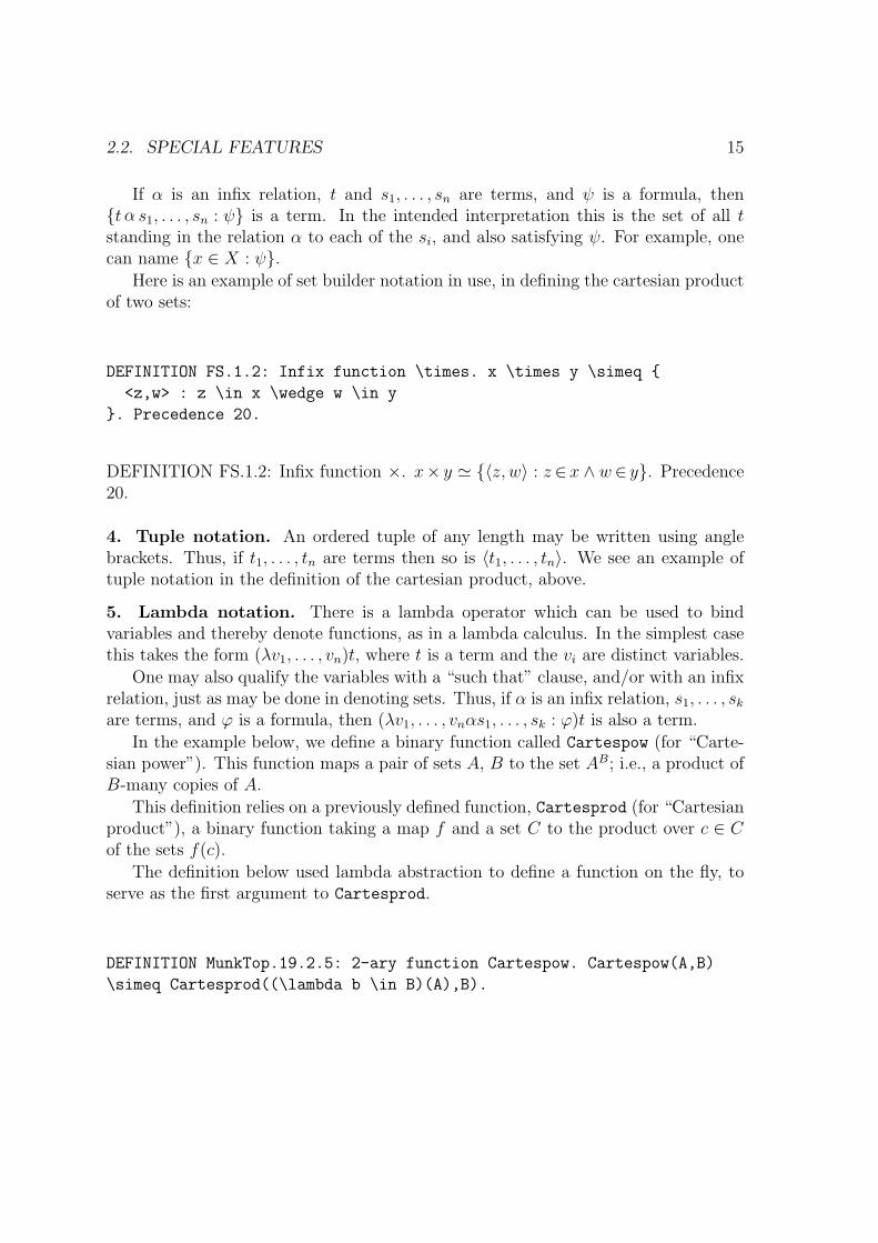
4. Tuple notation. An ordered tuple of any length may be written using anglebrackets. Thus, if t1, . . . , tn are terms then so is 〈t1, . . . , tn〉. We see an example oftuple notation in the definition of the cartesian product, above.
5. Lambda notation. There is a lambda operator which can be used to bindvariables and thereby denote functions, as in a lambda calculus. In the simplest casethis takes the form (λv1, . . . , vn)t, where t is a term and the vi are distinct variables.
One may also qualify the variables with a “such that” clause, and/or with an infixrelation, just as may be done in denoting sets. Thus, if α is an infix relation, s1, . . . , sk
are terms, and ϕ is a formula, then (λv1, . . . , vnαs1, . . . , sk : ϕ)t is also a term.
In the example below, we define a binary function called Cartespow (for “Carte-sian power”). This function maps a pair of sets A, B to the set AB; i.e., a product ofB-many copies of A.
This definition relies on a previously defined function, Cartesprod (for “Cartesianproduct”), a binary function taking a map f and a set C to the product over c ∈ Cof the sets f(c).
The definition below used lambda abstraction to define a function on the fly, toserve as the first argument to Cartesprod.
DEFINITION MunkTop.19.2.5: 2-ary function Cartespow. Cartespow(A,B)
\simeq Cartesprod((\lambda b \in B)(A),B).

16 CHAPTER 2. LPT, THE LANGUAGE OF PROOFLESS TEXT
DEFINITION MunkTop.19.2.5: 2-ary function Cartespow. Cartespow(A,B) 'Cartesprod((λb∈B)(A), B).
6. Unique existence, and qualified quantification. In addition to the usual ∀and ∃ quantifiers we also include ∃! for “there exists a unique”.
One may quantify not just variables but terms in general. In the intended inter-pretation, quantification over terms simply means quantification over all the variablesappearing in those terms.
Quantified terms may be further qualified, again, as in items above, with a “suchthat” clause, and/or with an infix relation.
For example, below we see a definition of what it means for a space to be sequen-tially compact. In it, we put a condition not merely on “all f ,” but rather on “all fin the set Maps(ω, X).”
DEFINITION MunkTop.28.3: 2-ary relation SEQCPT. If TOPSP[X,T] then
SEQCPT[X,T] \iff (\forall f \in Maps(\omega,X))
(\exists g : SUBSEQ[g,f])(
(\exists x \in X)(TOPCONV[g,x,T])
).
DEFINITION MunkTop.28.3: 2-ary relation SEQCPT. If TOPSP[X, T ] then SEQCPT[X, T ] ↔(∀f ∈ Maps(ω,X))(∃g : SUBSEQ[g, f ])((∃x∈X)(TOPCONV[g, x, T ])).
7. Description operator. Traditionally a description operator is another variablebinder. We generalize this much as we have generalized the quantifiers: In LPT thedescription operator may be used to bind any term, not just a variable. Furthermorethe term may be qualified with an infix relation.
Below we see a definition in which we have used the description operator ! to bindthe ordered pair 〈Y, T ′〉.
DEFINITION MunkTop.29.4: 2-ary function Oneptcompactification.
If TOPSP[X,T] then Oneptcompactification(X,T) \simeq
(!<Y,T’>)(
COMPACTIFICATION[Y,T’,X,T] \wedge Y \less X \approx_C 1_N
).
DEFINITION MunkTop.29.4: 2-ary function Oneptcompactification. If TOPSP[X, T ]then Oneptcompactification(X, T ) ' (! 〈Y, T ′〉)(COMPACTIFICATION[Y, T ′, X, T ] ∧Y \X ≈C 1N).

2.3. PARSING 17
2.3 Parsing
Let us review computer parsing methods and discuss the system that we use to parseLPT.
For the purposes of computer science, a language is nothing more than a set offinite strings over some alphabet Σ. The general problem of deciding membership ofa string in a language is undecidable (just take the language consisting of all stringsrepresenting halting Turing-machine/input pairs, with respect to some encoding).But there is a large class of languages for which there are standard algorithms todecide membership: namely, the class of languages specified by what is known as acontext-free grammar.
Languages in this class are actually more than just sets of strings; they havesyntactic structure. And the algorithms that decide membership in these languagesalso determine the syntactic structure of the input. These algorithms are calledparsers.
A context-free grammar or CFG is a special case of something more general, knownas a formal grammar. A formal grammar defines a language by giving production rulesby which all of the strings in the language can be “produced”, starting from a single“start symbol”. Formally, it is an ordered quadruple G = (N, Σ, P, S), where N iscalled the set of nonterminals, or nonterminal symbols, Σ is called the alphabet, orthe set of terminals, or terminal symbols, P is called the set of productions, and S iscalled the start symbol.
The sets N and Σ are disjoint. The start symbol S is an element of N . As forP , it is most easily described using standard computer science notation for sets ofstrings. If A and B are sets of symbols, then by A∗ we denote the set of all finitestrings of symbols taken from A (including the length zero “empty string” denotede), and by AB we denote the set of all strings consisting of one element of A followedby one element of B. These notations may be used in combination. The set P ofproductions is then some set of ordered pairs contained in
(N ∪ Σ)∗N(N ∪ Σ)∗ × (N ∪ Σ)∗,
and if (α, β) ∈ P we may express this by writing simply
α → β,
which is read, “α produces β”.In order to make use of this idea of “production” we define a binary relation ⇒ on
(N ∪ Σ)∗ so that for all α, β ∈ (N ∪ Σ)∗, we have α ⇒ β just in case there are some

18 CHAPTER 2. LPT, THE LANGUAGE OF PROOFLESS TEXT
γ, δ, ε, ζ in (N ∪ Σ)∗ such that α = γδε, β = γζε, and (δ, ζ) ∈ P . We then define ⇒∗
to be the transitive and reflexive closure of ⇒.
The language L(G) determined by a formal grammar G = (N, Σ, P, S) is thendefined to be the set of all α in Σ∗ such that S ⇒∗ α. Intuitively, you can reach thestring α by starting from the start symbol S and using the productions in P .
Let us return now to the grammars that are of particular interest to us, thecontext-free grammars or CFG’s. A CFG is any formal grammar in which the set Pof productions is contained in
N × (N ∪ Σ)∗.
The idea is that now the productions simply tell you what a given nonterminal symbolA ∈ N can produce; it is no longer possible to demand further that A be precededand/or followed by some particular elements of (N ∪ Σ)∗, i.e. that it be found ina certain “context”. CFG’s are the most important grammars in computer sciencebecause most important computer languages can be specified by them, and becausethere are efficient algorithms to parse the languages that they determine.
Of course, as one would expect, it is not as though we are designing parsingalgorithms on a grammar-by-grammar basis, taking a given grammar G and thendesigning an algorithm to parse the language that it determines, then taking the nextgrammar G′ and starting all over again. On the contrary, if CFG is the class of allcontext-free grammars then the general practice is to fix on some subclass A ⊆ CFGand to design a parsing algorithm that will work for any grammar G ∈ A.
This results in the development of computer programs called compiler compilers.You pass a formal grammar G belonging to the appropriate class A to a compilercompiler, and it compiles for you a compiler, which will parse the language of G. Thereader may wonder why it is not called a “parser compiler” instead. This is onlybecause a compiler is something more general than a parser, which involves a parserat its front end. A compiler compiler produces this more general kind of program,which one is free to use as though it were a mere parser.
Parsing algorithms that work for all of the grammars in CFG do exist; one popularcase is the Earley Algorithm, named after J. Earley, who invented it in 1970. Thereason that anyone bothers with algorithms that can handle only grammars belongingto proper subsetsA ⊂ CFG is that it is sometimes possible to design faster algorithms,if A is sufficiently restricted.
I have opted to use the Earley algorithm. Why not use something faster? A likelyalternative would be the LL(k) algorithms, which are commonly used in computerscience; for example, for parsing programming languages.
By LL(k) we mean an infinite class of algorithms. For any given positive integer

2.3. PARSING 19
k the LL(k) algorithm is designed to construct a left parse tree on the basis of nomore than k input tokens beyond the current input pointer. The first ‘L’ stands forthe left parse tree, and the other ‘L’ stands for the “lookahead” of at most k tokens.The runtime of the LL(k) algorithm is linear in the length of the input [3], but onlycertain grammars – known as the LL grammars – can be parsed.
Whether LPT has any LL grammar is not known to me. On the other hand, Ibelieve that the grammar that I have used for LPT is the grammar that one wouldmost naturally write down; and this grammar is certainly not LL, as I prove inAppendix B. Briefly, the problem stems from a choice point in the grammar at whicheither a term or a formula could come next. (Consider the sort of formula given inpoint 8 in Section 2.1.1.) Either of these nonterminals can begin with an arbitrarynumber of parentheses, and this means the grammar is not LL(k) for any k.
One response to this problem is to simply make k larger than the number of nestedparentheses that any human being would ever want to look at. But lookahead comesat a cost in the LL(k) algorithm. The size of the parse table used by the algorithmis in general, in the worst case, exponential in k [2].
Another solution would be to augment the basic LL(k) algorithm. It is possibleto parse arbitrarily nested parentheses, using a recursion stack [13]. But then welose the advantage of a tried-and-true algorithm, as produced directly by a compilercompiler, on the basis of a formal grammar.
Yet another possible response would be to search for an alternative grammar forLPT, one which was LL. But this would probably require that we warp the grammarthat we wanted to use quite a bit. There is an advantage to using a grammar whichis immediately and intuitively correct to a human eye.
My response has been to simply use the Earley Algorithm to parse LPT. Thealgorithm is described in detail in [3]. The Earley algorithm can parse any context-free grammar, and it has runtime at worst O(n3) (where n is the length of the input),and in fact runs in time O(n2) if the grammar happens to be unambiguous. This isa runtime which could possibly become restrictive for long inputs, such as computerprograms; but for input of the size of mathematical definitions it is no problem at all.In compiling my database of definitions the parser never ran for more than a coupleof seconds.
I have used a compiler compiler known as ACCENT: “A Compiler Compiler forthe ENTire class of context free grammars.” It is described in [14]. One passes toACCENT a description of the desired formal grammar, and it compiles a parser forthis grammar that implements the Earley Algorithm.

20 CHAPTER 2. LPT, THE LANGUAGE OF PROOFLESS TEXT
Chapter 3
First application: Translation
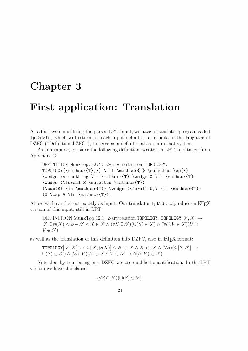
As a first system utilizing the parsed LPT input, we have a translator program calledlpt2dzfc, which will return for each input definition a formula of the language ofDZFC (“Definitional ZFC”), to serve as a definitional axiom in that system.
As an example, consider the following definition, written in LPT, and taken fromAppendix G:
DEFINITION MunkTop.12.1: 2-ary relation TOPOLOGY.
TOPOLOGY[\mathscrT,X] \iff \mathscrT \subseteq \wp(X)
\wedge \varnothing \in \mathscrT \wedge X \in \mathscrT
\wedge (\forall S \subseteq \mathscrT)
(\cup(S) \in \mathscrT) \wedge (\forall U,V \in \mathscrT)
(U \cap V \in \mathscrT).
Above we have the text exactly as input. Our translator lpt2dzfc produces a LATEXversion of this input, still in LPT:
DEFINITION MunkTop.12.1: 2-ary relation TOPOLOGY. TOPOLOGY[T , X] ↔T ⊆℘(X) ∧ ∅∈T ∧ X ∈T ∧ (∀S⊆T )(∪(S)∈T ) ∧ (∀U, V ∈T )(U ∩V ∈T ).
as well as the translation of this definition into DZFC, also in LATEX format:
TOPOLOGY[T , X] ↔ ⊆[T , ℘(X)] ∧ ∅ ∈ T ∧ X ∈ T ∧ (∀S)(⊆[S, T ] →∪(S) ∈ T ) ∧ (∀U, V )(U ∈ T ∧ V ∈ T → ∩(U, V ) ∈ T )
Note that by translating into DZFC we lose qualified quantification. In the LPTversion we have the clause,
(∀S⊆T )(∪(S)∈T ),
21
22 CHAPTER 3. FIRST APPLICATION: TRANSLATION
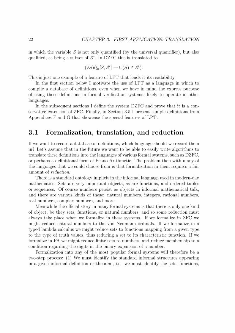
in which the variable S is not only quantified (by the universal quantifier), but alsoqualified, as being a subset of T . In DZFC this is translated to
(∀S)(⊆[S, T ] → ∪(S) ∈ T ).
This is just one example of a feature of LPT that lends it its readability.In the first section below I motivate the use of LPT as a language in which to
compile a database of definitions, even when we have in mind the express purposeof using those definitions in formal verification systems, likely to operate in otherlanguages.
In the subsequent sections I define the system DZFC and prove that it is a con-servative extension of ZFC. Finally, in Section 3.5 I present sample definitions fromAppendices F and G that showcase the special features of LPT.
3.1 Formalization, translation, and reduction
If we want to record a database of definitions, which language should we record themin? Let’s assume that in the future we want to be able to easily write algorithms totranslate these definitions into the languages of various formal systems, such as DZFC,or perhaps a definitional form of Peano Arithmetic. The problem then with many ofthe languages that we could choose from is that formalization in them requires a fairamount of reduction.
There is a standard ontology implicit in the informal language used in modern-daymathematics. Sets are very important objects, as are functions, and ordered tuplesor sequences. Of course numbers persist as objects in informal mathematical talk,and there are various kinds of these: natural numbers, integers, rational numbers,real numbers, complex numbers, and more.
Meanwhile the official story in many formal systems is that there is only one kindof object, be they sets, functions, or natural numbers, and so some reduction mustalways take place when we formalize in these systems. If we formalize in ZFC wemight reduce natural numbers to the von Neumann ordinals. If we formalize in atyped lambda calculus we might reduce sets to functions mapping from a given typeto the type of truth values, thus reducing a set to its characteristic function. If weformalize in PA we might reduce finite sets to numbers, and reduce membership to acondition regarding the digits in the binary expansion of a number.
Formalization into any of the most popular formal systems will therefore be atwo-step process: (1) We must identify the standard informal structures appearingin a given informal definition or theorem, i.e. we must identify the sets, functions,

3.2. A TRANSLATION TARGET SYSTEM 23
tuples, numbers, etc. in terms of which the statement is given. Then (2) We musttranslate into the formal system, reducing the standard structures as necessary.
A language in which formalization requires a lot of reduction will not be a goodlanguage for our database of definitions, since reduction can be hard to reverse. Thismeans that it would be hard to write algorithms to translate from the databaselanguage into various other languages.
So what we want is a language in which we can formalize informal definitions,and yet one which requires a minimum of reduction. It will be easy later on to setup mechanical translations from this language into others. Clearly, a language thatrequires little reduction will just be one that features locutions to accommodate talkof as many as possible of the sorts of objects that belong to the standard informalontology of modern-day mathematical discourse. This is just what LPT provides. Itgives ways to denote sets, functions, and tuples.
But why not just record definitions in natural language? Well, as of now goodalgorithms for natural language processing are still very experimental. But that’snot really the important point anyway. We may very well have good algorithmssoon. More importantly, I anticipate that if we had a system to translate directlyfrom natural language into, say, the language of DZFC, it would probably work bypassing through a stage in which it had refined an informal definition into somethinga lot like what we get when we translate into LPT by hand. Standard techniques offormalization work by fixing on the standard structures in the informal ontology andthen reducing these. We will want to continue using these techniques, and so we willcontinue to want to translate informal definitions into standard formal systems by firstnoting which of these structures occur in them, and then formalizing in terms of these.If we are going to pass through a representation like what we get in LPT anyway, thenwe are not losing anything (at least not much) by recording our definitions directlyin LPT.
So much is true at least for mathematical text written expressly for computerstorage. Meanwhile, we may also wish to produce electronic versions of existingtexts, for MKM purposes. In that case, a natural language parser would indeed bedesirable.
3.2 A translation target system
We hope that LPT will be amenable to translation into most any popular formalsystem, since formalization in LPT should require little reduction. On the otherhand, many of the definitions that we may encounter in textbooks, at least those

24 CHAPTER 3. FIRST APPLICATION: TRANSLATION
given in a foundational development of mathematics, will already involve quite a bitof reduction, of one kind or another. If we are following a set-theoretic development ofthe number systems from N on up to C for example, then the definitions will involvereductions that we would not want to use if, say, we were developing mathematics inarithmetic instead of in set theory. In this way our choice of definitions to formalizedoes represent some loss of the general applicability of LPT.
In the definitions that I compile in Appendices F and G I follow a set-theoreticdevelopment. Accordingly, we need a computer program to translate from LPT intosome system of set theory. ZFC would be the most obvious choice, but in fact asystem that offers a little bit more will work much better for formalizers wishing towork (ultimately) in ZFC.
Even an informal proof of modest length or complexity can be essentially unintelli-gible to a human reader if fully formalized in ZFC. We lose the advantages of definedfunctions and relations if we try to work directly in ZFC. In order to formalize agiven proof that uses defined functions f1, . . . , fn and defined relations R1, . . . , Rm,it makes sense to work in a definitional extension of ZFC that features function andrelation strings to stand for the fi and the Rj, and definitional axioms to allow formaldeduction with these functions and relations. The definitional axioms for the definedfunctions in turn demand that we provide a description operator.
These considerations motivate the design of a program to translate from LPT toDZFC, rather than to ZFC itself. My program lpt2dzfc serves this purpose. Itis impractical to set up a further translation, from DZFC to ZFC, since the formergives an iterated exponential speedup over the latter. This means that it is impossibleto bound the increase in length by any fixed stack of exponentials [5]. Fortunatelyhowever, DZFC is a conservative extension of ZFC, as I prove in the sections below.This means that formalizers wishing to ground theorems in the axioms of ZFC mayinstead work in DZFC, and simply invoke conservativity.
3.3 DZFC
To get DZFC we just add to ZFC those features needed to work with defined functionsand relations. Primarily this means the expansion of the language to include infinitecollections of function and relation strings, as well as the inclusion of a descriptionoperator, ι.
We also design DZFC to use free logic, i.e., logic in which terms may fail todenote. In this we follow Feferman [8]. This allows us to make function definitionsmore natural, by leaving functions undefined at certain arguments. For example, in

3.3. DZFC 25
developing arithmetic we need not define division by zero. In order to use free logicwe include in DZFC a definedness predicate ↓, and a partial equality relation '.
DZFC is our basic definitional system. If σ is a set of function and relation symbolsthen we write DZFC(σ) for the system obtained by adding to DZFC a definitionalaxiom for each symbol in σ.
Given a set σ = f1, . . . , fn, R1, . . . , Rm of defined function and relation symbols,the axioms and rules of inference for DZFC(σ) are as follows.
I. Propositional Axioms and Rules
(i) Axioms: All substitution instances of tautologies.
(ii) Rules:
MPA → B A
B
II. Quantificational Axioms and Rules
(i) Axioms:∀ − Ax ∀xA(x) ∧ (t↓) → A(t)
∃ − Ax A(t) ∧ (t↓) → ∃xA(x)
where t is free for x in A.
(ii) Rules:
∀IB → A(x)
B → ∀xA(x)
∃EA(x) → B
∃xA(x) → B
where ‘ x ′ is not free in B.
III. Equality and Substitution Axioms
(i) x = x
(ii) s = t → t = s
(iii) r = s ∧ s = t → r = t
(iv) s1 ∈ s2 ∧ ~s = ~t → t1 ∈ t2
(v) (s↓) ∧ s = t → (t↓)

26 CHAPTER 3. FIRST APPLICATION: TRANSLATION
(vi) s ' t ↔ ((s↓) ∨ (t↓) → s = t)
(vii) Rj(~s) ∧ ~s = ~t → Rj(~t)
(viii) ~s = ~t → fi(~s) ' fi(~t)
IV. Set Axioms. The usual axioms of ZFC, where the formulas in the Separationand Replacement schemata range over all formulas of DZFC.
V. Description Axiom
DES y = (ιx)A(x) ↔ ∀z(A(z) ↔ z = y).
VI. Definedness Axioms
(i) x↓(ii) ∅↓(iii) s = t → (s↓) ∧ (t↓)(iv) s ∈ t → (s↓) ∧ (t↓)(v) fi↓ for nullary functions fi
(vi) fi(~t)↓ → (~t↓)(vii) Rj(~t) → (~t↓)
VII. Definitional Axioms. For each function symbol fi we add a definitional axiomof the form fi~x ' (ιy)Afi
(~x, y), where fk does not appear in the formula Afifor
k ≥ i. Likewise, for each relation symbol Rj we add a definitional axiom of theform Rj(~x) ↔ φRj
(~x), where Rk does not appear in the formula φRjfor k ≥ j.
f1~x ' (ιy)Af1(~x, y)...
fn~x ' (ιy)Afn(~x, y)
R1(~x) ↔ φR1(~x)...
Rm(~x) ↔ φRm(~x)
3.4. CONSERVATIVITY 27
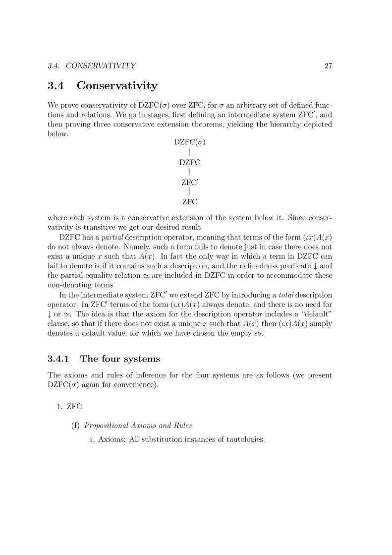
3.4 Conservativity
We prove conservativity of DZFC(σ) over ZFC, for σ an arbitrary set of defined func-tions and relations. We go in stages, first defining an intermediate system ZFC′, andthen proving three conservative extension theorems, yielding the hierarchy depictedbelow:
ZFC
ZFC′
DZFC
DZFC(σ)
........
........
........
..
........
........
........
..
........
........
........
..
where each system is a conservative extension of the system below it. Since conser-vativity is transitive we get our desired result.
DZFC has a partial description operator, meaning that terms of the form (ιx)A(x)do not always denote. Namely, such a term fails to denote just in case there does notexist a unique x such that A(x). In fact the only way in which a term in DZFC canfail to denote is if it contains such a description, and the definedness predicate ↓ andthe partial equality relation ' are included in DZFC in order to accommodate thesenon-denoting terms.
In the intermediate system ZFC′ we extend ZFC by introducing a total descriptionoperator. In ZFC′ terms of the form (ιx)A(x) always denote, and there is no need for↓ or '. The idea is that the axiom for the description operator includes a “default”clause, so that if there does not exist a unique x such that A(x) then (ιx)A(x) simplydenotes a default value, for which we have chosen the empty set.
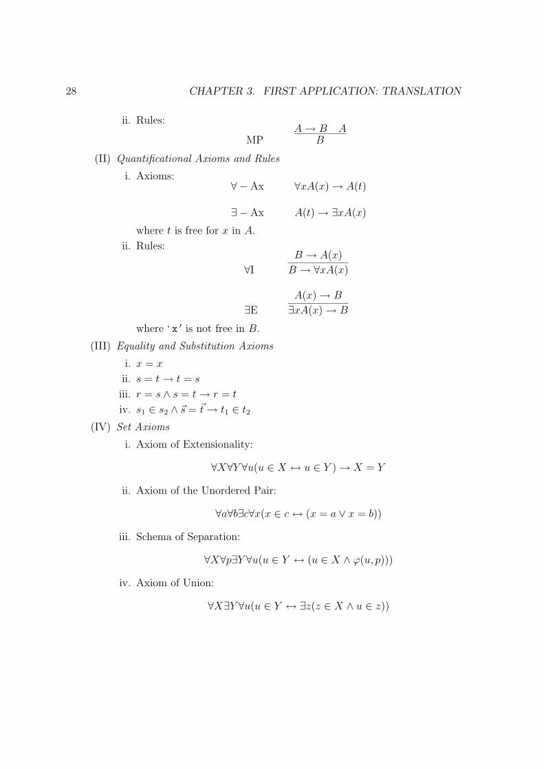
3.4.1 The four systems
The axioms and rules of inference for the four systems are as follows (we presentDZFC(σ) again for convenience).
1. ZFC.
(I) Propositional Axioms and Rules
i. Axioms: All substitution instances of tautologies.
28 CHAPTER 3. FIRST APPLICATION: TRANSLATION
ii. Rules:
MPA → B A
B
(II) Quantificational Axioms and Rules
i. Axioms:∀ − Ax ∀xA(x) → A(t)
∃ − Ax A(t) → ∃xA(x)
where t is free for x in A.
ii. Rules:
∀IB → A(x)
B → ∀xA(x)
∃EA(x) → B
∃xA(x) → B
where ‘ x ′ is not free in B.
(III) Equality and Substitution Axioms
i. x = x
ii. s = t → t = s
iii. r = s ∧ s = t → r = t
iv. s1 ∈ s2 ∧ ~s = ~t → t1 ∈ t2
(IV) Set Axioms
i. Axiom of Extensionality:
∀X∀Y ∀u(u ∈ X ↔ u ∈ Y ) → X = Y
ii. Axiom of the Unordered Pair:
∀a∀b∃c∀x(x ∈ c ↔ (x = a ∨ x = b))
iii. Schema of Separation:
∀X∀p∃Y ∀u(u ∈ Y ↔ (u ∈ X ∧ ϕ(u, p)))
iv. Axiom of Union:
∀X∃Y ∀u(u ∈ Y ↔ ∃z(z ∈ X ∧ u ∈ z))

3.4. CONSERVATIVITY 29
v. Axiom of the Power Set:
∀X∃Y ∀u(u ∈ Y ↔ ∀z(z ∈ u → z ∈ X))
vi. Axiom of Infinity:
∃S(∅ ∈ S ∧ (∀x ∈ S)(x ∪ x ∈ S))
vii. Schema of Replacement:
∀p [∀x∀y∀z(ϕ(x, y, p) = ϕ(x, z, p) → y = z)
→ ∀X∃Y ∀y(y ∈ Y ↔ (∃x ∈ X)(ϕ(x, y, p)))]
viii. Axiom of Foundation:
∀S(S 6= ∅→ (∃x ∈ S)(S ∩ x = ∅))
ix. Axiom of Choice:
∀A [∀x∀y(x ∈ A ∧ y ∈ A → x ∩ y = ∅ ∧ x 6= ∅)
→ ∃C∀x(x ∈ A → ∃y∀z(z ∈ x ∩ C ↔ z = y)))]
2. ZFC′. To the language we add the symbol ι, a description operator. It will beaxiomatized so that it is total, not partial; thus, (ιx)A(x) is always defined, forany formula A. The idea is that if in fact there is a unique x such that A(x)then (ιx)A(x) will return this very x; otherwise it will return a default value,namely, the empty set ∅. The axioms and rules are as follows.
(I) Propositional Axioms and Rules. Same as ZFC.
(II) Quantificational Axioms and Rules. Same as ZFC.
(III) Equality and Substitution Axioms. Same as ZFC.
(IV) Set Axioms. Expand the separation and replacement schemata so that ϕis any formula of the new language.
(V) Description Axiom
t−DES y = (ιx)A(x) ↔ [∀z(A(z) ↔ z = y) ∨ (¬∃!zA(z) ∧ y = ∅)].

30 CHAPTER 3. FIRST APPLICATION: TRANSLATION
3. DZFC. The language is the same as for ZFC′, except that we add a definednesspredicate ↓, and a partial equality symbol '. The description axiom is changedso that now ι will be a partial description operator instead of total. This meansthat we remove the “defaulting mechanism”, so that now (ιx)A(x) is simply“undefined” if there is not a unique x such that A(x).
What it really means to say that now some terms will be “undefined” amountsprimarily to a change in the quantificational axioms: they become more strin-gent, their antecedents now requiring that the terms involved be “defined”.Here, a term is “defined” just in case it satisfies the new definedness predicate↓. Thus we also need new axioms with which to infer this definedness.
Axioms and rules are as follows.
(I) Propositional Axioms and Rules. Same as ZFC′.
(II) Quantificational Axioms and Rules. Rules the same as ZFC′. The axiomsbecome:
∀ − Ax ∀xA(x) ∧ (t↓) → A(t)
∃ − Ax A(t) ∧ (t↓) → ∃xA(x)
where t is free for x in A.
(III) Equality and Substitution Axioms. Those of ZFC′, plus:
(s↓) ∧ s = t → (t↓)
s ' t ↔ ((s↓) ∨ (t↓) → s = t)
(IV) Set Axioms. Expand the separation and replacement schemata so that ϕis any formula of the new language.
(V) Description Axiom
p−DES y = (ιx)A(x) ↔ ∀z(A(z) ↔ z = y).
(VI) Definedness Axioms
i. x↓ii. ∅↓iii. s = t → (s↓) ∧ (t↓)iv. s ∈ t → (s↓) ∧ (t↓)

3.4. CONSERVATIVITY 31
4. DZFC(σ). We have a set σ = f1, . . . , fn, R1, . . . , Rm of function and relationsymbols to be defined. For each function symbol fi we add a definitional axiomof the form fi~x ' (ιy)Afi
(~x, y), where fk does not appear in the formula Afi
for k ≥ i. For each relation symbol Rj we add a definitional axiom of the formRj(~x) ↔ φRj
(~x), where Rk does not appear in the formula φRjfor k ≥ j.
(I) Propositional Axioms and Rules. Same as DZFC.
(II) Quantificational Axioms and Rules. Same as DZFC.
(III) Equality and Substitution Axioms. Those of DZFC, plus:
Rj(~s) ∧ ~s = ~t → Rj(~t)
~s = ~t → fi(~s) ' fi(~t)
(IV) Set Axioms. Same as DZFC.
(V) Description Axiom. Same as DZFC.
(VI) Definedness Axioms. Those of DZFC, plus:
fi↓, fornullaryfunctionsfi
fi(~t)↓ → (~t↓)Rj(~t) → (~t↓)
(VII) Definitional Axioms. As described above,
f1~x ' (ιy)Af1(~x, y)...
fn~x ' (ιy)Afn(~x, y)
R1(~x) ↔ φR1(~x)...
Rm(~x) ↔ φRm(~x)
3.4.2 The extension theorems
Our first theorem states that ZFC ′ is a conservative extension of ZFC. This is thefirst among three conservative extension theorems that we have to prove, and thebasic strategy will be the same each time.

32 CHAPTER 3. FIRST APPLICATION: TRANSLATION
To show that a formal theory T ′ is a conservative extension of a subsystem T wewill define a translation ∗ from the formulas of T ′ to the formulas of T in such a waythat whenever a formula A of T ′ is also a formula of the subsystem T then A∗ isprovably equivalent to A in the system T . Then we just need to prove that for everytheorem A of T ′, A∗ is a theorem of T .
We use induction on the length of the shortest proof of A in T ′. Since the shortestany proof can be is one line, and since the only formulas with one-line proofs areaxioms, this means that the base step consists precisely of showing that for everyaxiom A of T ′, A∗ is a theorem of T .
The induction step is easy, and we get it out of the way right now. Suppose A isa theorem of T ′ whose shortest proof is n lines. Then there is some rule of inferenceR in T ′, and some set N ⊆ 1, 2, . . . , n− 1 such that A can be inferred in T ′ byapplying rule R to the lines of the proof whose line numbers are in N . Let us denotethe formula on line k by Bk. Then for each k ∈ N , Bk is a theorem of T ′, andtherefore, by the inductive hypothesis, B∗
k is a theorem of T . It would suffice then toshow that A∗ follows in T from B∗
kk∈N .Thus, for the induction step it suffices to show that for all rules of inference R of
T ′, all sets H of hypotheses, and all sentences A, we have
HA
R ⇒ H∗ `T A∗. (3.1)
All four of our logical systems have the same three rules of inference: the onepropositional rule of modus ponens, and the two quantificational rules of universalintroduction and existential elimination. Therefore (3.1) holds provided the ∗ trans-lation meets two criteria:
i. ∗ commutes with → and with the quantifiers ∀ and ∃, and
ii. if ∗ introduces any free variables they are always fresh.
In fact every translation we define below will meet these two criteria, so the inductionstep is done for each of our conservative extension theorems. In each case we nowneed only show the base step, that each axiom of T ′ translates to a theorem of T .
We return now to our first goal, of proving that ZFC ′ is a conservative extensionof ZFC. We define a translation, and prove in several lemmas that the axioms ofZFC ′ translate to theorems of ZFC.
The translation ∗ from ZFC ′ to ZFC will make use of two auxiliary functions,one the “underscore” function, and the other a function called ∆. We define all three
3.4. CONSERVATIVITY 33
simultaneously. All of these techniques and notations come from [16], Chapter 2,Section 7.
The ∆ function will be defined on terms t, and for each term t will return a formula∆(t). We will extend the domain of ∆ to the set of all finite sequences ~t of terms bythe convention that
∆(~t) =
|~t|∧i=1
∆(ti).
In this and later sections we will use other functions similar to ∆ and will use thesame convention for these, without comment.
We also use an indexing of the occurrences of the description operator ι in for-mulas. Thus, we write (ιy)B(y) instead as (ιky)B(y) with k an index. All indicesare distinct, and beyond this constraint our proof is independent of the manner ofindexing.
For each occurrence ιk of the description operator we will be introducing a variable,assumed to be fresh, denoted yk. This correspondence will be implicit when weintroduce a whole sequence ~y of variables corresponding to a formula containingseveral occurrences of the description operator.
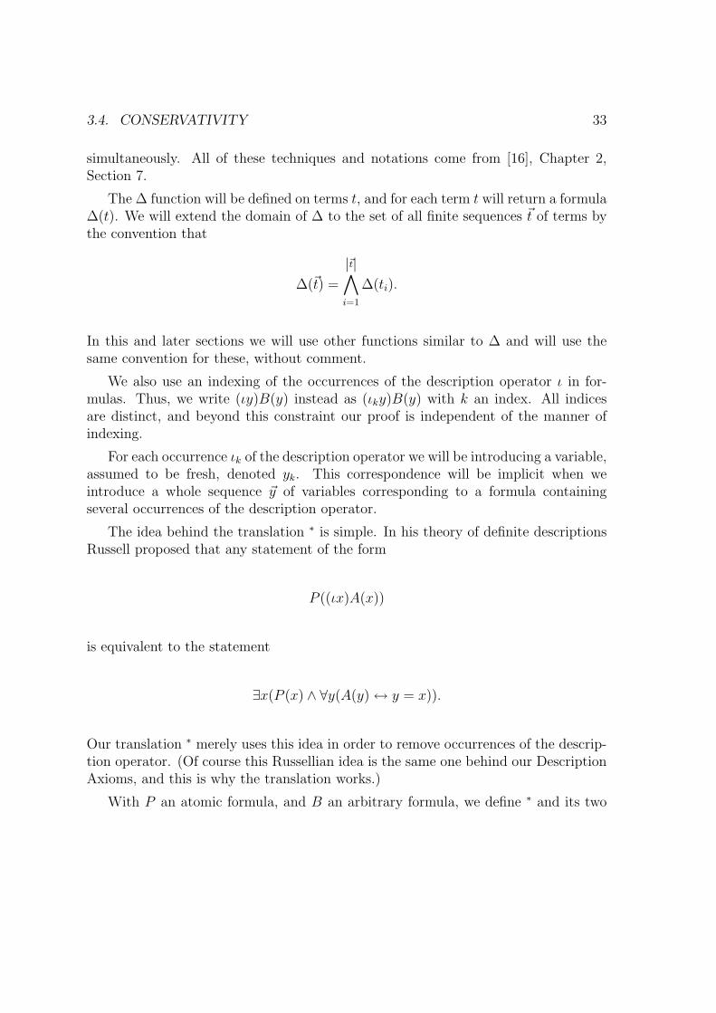
The idea behind the translation ∗ is simple. In his theory of definite descriptionsRussell proposed that any statement of the form
P ((ιx)A(x))
is equivalent to the statement
∃x(P (x) ∧ ∀y(A(y) ↔ y = x)).
Our translation ∗ merely uses this idea in order to remove occurrences of the descrip-tion operator. (Of course this Russellian idea is the same one behind our DescriptionAxioms, and this is why the translation works.)
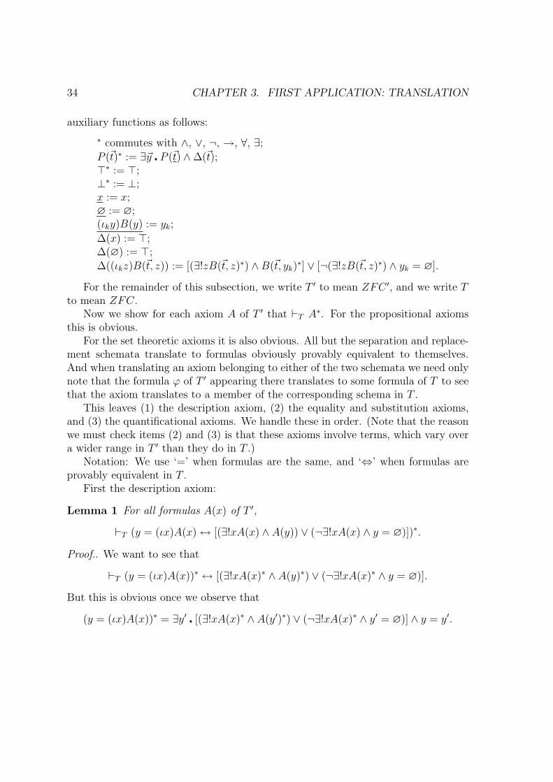
With P an atomic formula, and B an arbitrary formula, we define ∗ and its two
34 CHAPTER 3. FIRST APPLICATION: TRANSLATION
auxiliary functions as follows:
∗ commutes with ∧, ∨, ¬, →, ∀, ∃;P (~t)∗ := ∃~y ¦ P (~t) ∧∆(~t);>∗ := >;⊥∗ := ⊥;x := x;∅ := ∅;(ιky)B(y) := yk;
∆(x) := >;∆(∅) := >;
∆((ιkz)B(~t, z)) := [(∃!zB(~t, z)∗) ∧B(~t, yk)∗] ∨ [¬(∃!zB(~t, z)∗) ∧ yk = ∅].
For the remainder of this subsection, we write T ′ to mean ZFC ′, and we write Tto mean ZFC.
Now we show for each axiom A of T ′ that `T A∗. For the propositional axiomsthis is obvious.
For the set theoretic axioms it is also obvious. All but the separation and replace-ment schemata translate to formulas obviously provably equivalent to themselves.And when translating an axiom belonging to either of the two schemata we need onlynote that the formula ϕ of T ′ appearing there translates to some formula of T to seethat the axiom translates to a member of the corresponding schema in T .
This leaves (1) the description axiom, (2) the equality and substitution axioms,and (3) the quantificational axioms. We handle these in order. (Note that the reasonwe must check items (2) and (3) is that these axioms involve terms, which vary overa wider range in T ′ than they do in T .)
Notation: We use ‘=’ when formulas are the same, and ‘⇔’ when formulas areprovably equivalent in T .
First the description axiom:
Lemma 1 For all formulas A(x) of T ′,
`T (y = (ιx)A(x) ↔ [(∃!xA(x) ∧ A(y)) ∨ (¬∃!xA(x) ∧ y = ∅)])∗.
Proof.. We want to see that
`T (y = (ιx)A(x))∗ ↔ [(∃!xA(x)∗ ∧ A(y)∗) ∨ (¬∃!xA(x)∗ ∧ y = ∅)].
But this is obvious once we observe that
(y = (ιx)A(x))∗ = ∃y′ ¦ [(∃!xA(x)∗ ∧ A(y′)∗) ∨ (¬∃!xA(x)∗ ∧ y′ = ∅)] ∧ y = y′.

3.4. CONSERVATIVITY 35
¤
Next we consider the four equality and substitution axioms. For the first of these,the desired result is immediate. We will examine the second. The third and fourthare similar.
Lemma 2 For any terms s and t of T ′, we have `T (s = t → t = s)∗.
Proof. If both s and t are variables or constants the result is trivial. Supposings = (ιz)B(z) and t is a variable or a constant, we have
(s = t)∗ ⇔ ∃y ¦ y = t ∧∆((ιzB(z))
and(t = s)∗ ⇔ ∃y ¦ t = y ∧∆((ιzB(z))
and clearly T proves that the one implies the other.Finally, supposing s = (ιz)B(z), and t = (ιz)C(z) we have
(s = t)∗ ⇔ ∃y1, y2 ¦ y1 = y2 ∧∆((ιzB(z)) ∧∆((ιzC(z))
and(t = s)∗ ⇔ ∃y1, y2 ¦ y2 = y1 ∧∆((ιzB(z)) ∧∆((ιzC(z))
and once again the result is clear. ¤
Finally we must show that the two quantificational axioms of T ′ translate totheorems of T . In order to do this we define a second translation, †. This translationwill make use of the same Russellian theory of definite descriptions, adding clausesto deal with existence and uniqueness. The only difference is that whereas the ∗
translation kept these extra clauses conjoined right beside the atomic formulas, the† translation will put these clauses on the outside of the whole formula. In the nextlemma we establish that for any formula in T ′, its two translations into T , under ∗
and under †, are provably equivalent in T .For the † translation we use an auxiliary function Γ slightly different from ∆
(notice that there are no ∗’s on the right-hand side in its definition below); we use thesame underscore function. For an arbitrary formula A we write A(~t) to mean that ~tis the sequence of all distinct terms appearing anywhere in the formula A, in orderfrom left to right. A bound variable is not considered to be a term. So, for example,if we had
A ≡ (x ∈ y) ∧ (x 6∈ ∅) ∧ (y = (ιz)B(~w, z)) ∧ ∃u(u = ∅)

36 CHAPTER 3. FIRST APPLICATION: TRANSLATION
then we would writeA ≡ A(x, y,∅, (ιz)B(~w, z), ~w).
Let A and B be arbitrary formulas. The definition of † is as follows.
A(~t)† := ∃~y ¦ A(~t) ∧ Γ(~t);>† := >;⊥† := ⊥;x := x;∅ := ∅;(ιky)B(y) := yk;
Γ(x) := >;Γ(∅) := >;
Γ((ιkz)B(~t, z)) := [(∃!zB(~t, z)) ∧B(~t, yk)] ∨ [¬(∃!zB(~t, z)) ∧ yk = ∅].
Lemma 3 For every formula A of T ′, we have
`T A∗ ↔ A†. (3.2)
Proof. Again following [16], Chapter 2, Section 7, we begin by defining a “degree” δon the formulas and terms of T ′ as follows. With B and C any formulas, and P anatomic formula, we define:
δ(x) := 0;δ(∅) := 0;δ((ιz)B(z)) := 1 + δ(B(z));
δ(P (~t)) := δ(~t) := max(δ(t1), . . . , δ(tn));δ(⊥) := 0;δ(>) := 0;δ(¬B) := 1 + δ(B);δ(B C) := 1 + max(δ(B), δ(C))for ∈ ∧,∨,→ ;δ(∀xB) = δ(∃xB) := 1 + δ(B).
The proof is by complete induction on δ(A).Base step: δ(A) = 0. Then either A = >, A = ⊥, or A = P (x,~v) for some
variables ~v = v1, . . . , vn distinct from x and some atomic formula P . In all of thesecases the result is obvious.
Induction step: δ(A) = n + 1. There are seven cases to consider:
i. A = B ∨ C,

3.4. CONSERVATIVITY 37
ii. A = B ∧ C,
iii. A = B → C,
iv. A = ¬B,
v. A = ∃zB,
vi. A = ∀zB, and
vii. A = P (~t).
In the first six cases we use the induction hypothesis and the fact that ∗ commuteswith the logical connectives and quantifiers to reduce to the goal of showing that
i. `L A† ↔ B† ∨ C†,
ii. `L A† ↔ B† ∧ C†,
iii. `L A† ↔ B† → C†,
iv. `L A† ↔ ¬B†,
v. `L A† ↔ ∃zB†, and
vi. `L A† ↔ ∀zB†.
All six cases are easy. Finally, case (vii), in which A is atomic, is obvious. ¤
At last we want to show that for every quantificational axiom A of T ′, we have`T A∗. But by lemma 3.2 it is enough to show that `T A†. Therefore we will provethe following lemma.
Lemma 4 For all formulas A of T ′ and terms t of T ′ such that t is free for x in A,we have
`T ∀xA† → ([t/x]A)† (3.3)
and`T ([t/x]A)† → ∃xA†. (3.4)
Proof. Since ([t/x]A)† is provably equivalent in T to ∃y ¦ [y/x]A† ∧ Γ(t), (3.4) followsimmediately. To get (3.3) we use a case analysis in T on (∃!zC(z)) ∨ ¬(∃!zC(z)),where t = (ιz)C(z). ¤
This completes our first conservative extension theorem.
Theorem 5 ZFC′ is a conservative extension of ZFC.

38 CHAPTER 3. FIRST APPLICATION: TRANSLATION
3.4.3 Second extension
Next we prove that DZFC is a conservative extension of ZFC′. The overall structureof the proof is the same as in the last section. This time we define the followingtranslation from DZFC to ZFC′.
† commutes with ∧, ∨, ¬, →, ∀, ∃;P (~t)† := P (~t) ∧ (~t↓)†, forP (~t) 6≡ (~t↓);(x↓)† := >;((ιx)B(x)↓)† := ∃!xB(x)†;x := x;(ιx)B(x) := (ιx)B(x)†.
Now we check that the axioms of DZFC translate to provable formulas of ZFC′.As in the last section, the propositional axioms and the set axioms are obvious.
We write T ∗ for DZFC, and T ′ for ZFC′.
Lemma 6 The translation of the description axiom of T ∗ is provable in T ′.
Proof. The translation of (ιx)A(x) = y ↔ ∀x[A(x) ↔ x = y] is provably equivalentto
(ιx)A(x)† = y ∧ ∃!xA(x)† ↔ ∀x[A(x)† ↔ x = y].
And, given the description axiom of T ′, this last is provably equivalent in T ′ to
[∀z(A(z)† ↔ z = y) ∨ (¬∃!zA(z)† ∧ y = ∅)] ∧ ∃!xA(x)† ↔ ∀x[A(x)† ↔ x = y],
which clearly T ′ proves. ¤
We turn now to the equality axioms.
Lemma 7 For all terms s, t of T ∗, we have T ′ ` (s = t → t = s)†.
Proof. Whatever s and t are, we have
(s = t → t = s)† ≡ s = t ∧ (s↓)† ∧ (t↓)† → t = s ∧ (t↓)† ∧ (s↓)†
and clearly T ′ proves the left-hand side. ¤
Lemma 8 For all terms r, s, t of T ∗, we have T ′ ` (r = s ∧ s = t → r = t)†.

3.4. CONSERVATIVITY 39
Proof is similar.Next the substitution axioms.
Lemma 9 T ′ ` (R(~s) ∧ ~s = ~t → R(~t))†.
Proof.
(R(~s) ∧ ~s = ~t → R(~t))† ⇔ R(~s) ∧ (~s↓)† ∧ ~s = ~t ∧ (~t↓)† → R(~t) ∧ (~t↓)†
and the left-hand side follows from substitution in T ′. ¤
It is obvious from our choice of translation that the definedness axioms translateto provable formulas in T ′.
Finally we come to the quantificational axioms. First we prove a supportinglemma (which makes up the bulk of this section).
Lemma 10 For all formulas A and terms t of T ∗, if x is free in A and t is free forx in A, then T ′ ` [t/x](A†) ∧ (t↓)† → ([t/x]A)†.
Proof. It suffices to prove the lemma under the additional assumption that A is innegation-normal form (¬ appears only immediately before atomic formulae), and doesnot contain →. Thus we begin by defining a degree δ on the formulas and terms ofT ∗ as follows:
δ(x) := 0;δ((ιx)B(x)) := 1 + δ(B(x));
δ(P (~t)) := δ(~t);δ(¬B) := δ(B);δ(B C) := 1 + max(δ(B), δ(C)), for ∈ ∧,∨ ;δ(∀xB) = δ(∃xB) := 1 + δ(B).
The proof is by complete induction on δ(A).Base step: δ(A) = 0. There are two cases to consider:
i. A ≡ P (x,~v), and
ii. A ≡ ¬P (x,~v).
We enumerate them below.

40 CHAPTER 3. FIRST APPLICATION: TRANSLATION
i. First we compute that
[t/x](A†) ≡ [t/x](P (x,~v)†)
≡ [t/x](P (x,~v) ∧ (x↓)† ∧ (~v↓)†)⇔ [t/x]P (x,~v)
≡ P (t, ~v)
and then that
([t/x]A)† ≡ ([t/x]P (x,~v))†
≡ P (t, ~v)†
≡ P (t, ~v) ∧ (t↓)† ∧ (~v↓)†⇔ P (t, ~v) ∧ (t↓)†
Thus T ′ ` [t/x](A†) ∧ (t↓)† → ([t/x]A)† is just
T ′ ` P (t, ~v) ∧ (t↓)† → P (t, ~v) ∧ (t↓)†.
ii. Now we have A ≡ ¬P (x,~v). This time the (t↓)† conjunct is really not needed,as we find:
[t/x](A†) ≡ [t/x](¬P (x,~v)†)
≡ [t/x]¬(P (x,~v) ∧ (x↓)† ∧ (~v↓)†)⇔ [t/x]¬P (x,~v)
≡ ¬P (t, ~v),
while
([t/x]A)† ≡ ([t/x]¬P (x,~v))†
≡ ¬P (t, ~v)†
≡ ¬(P (t, ~v) ∧ (t↓)† ∧ (~v↓)†)⇔ ¬P (t, ~v) ∨ ¬(t↓)†.
Of course T ′ ` ¬P (t, ~v) → ¬P (t, ~v). And we can strengthen the antecedent andweaken the consequent to get
T ′ ` ¬P (t, ~v) ∧ (t↓)† → ¬P (t, ~v) ∨ ¬(t↓)†
which is T ′ ` [t/x](A†) ∧ (t↓)† → ([t/x]A)† in this case.

3.4. CONSERVATIVITY 41
Induction step: δ(A) = n + 1. There are six cases to consider:
i. A ≡ B ∨ C,
ii. A ≡ B ∧ C,
iii. A ≡ ∃zB,
iv. A ≡ ∀zB,
v. A ≡ P (~s), and
vi. A ≡ ¬P (~s).
We enumerate them below. The first four cases are trivial. The fifth case is wherewe do the interesting work; the sixth case is similar.
i. A ≡ B ∨ C, with δ(B), δ(C) ≤ n. We begin by computing [t/x](A†) and([t/x]A)†. First
[t/x](A†) ≡ [t/x]((B ∨ C)†)
≡ [t/x](B† ∨ C†)
≡ [t/x](B†) ∨ [t/x](C†),
and then
([t/x]A)† ≡ ([t/x](B ∨ C))†
≡ ([t/x]B ∨ [t/x]C)†
≡ ([t/x]B)† ∨ ([t/x]C)†.
By the inductive hypothesis we have
T ′ ` [t/x](B†) ∧ (t↓)† → ([t/x]B)†
andT ′ ` [t/x](C†) ∧ (t↓)† → ([t/x]C)†
so if we defineD := [t/x](B†),
E := [t/x](C†),
F := ([t/x]B)†,
42 CHAPTER 3. FIRST APPLICATION: TRANSLATION
G := ([t/x]C)†,
H := (t↓)†,then we have
T ′ ` D ∧H → F
andT ′ ` E ∧H → G
and wantT ′ ` (D ∨ E) ∧H → (F ∨G),
which is easy to derive.
ii. A ≡ B ∧ C. Similar, and easier.
iii. A ≡ ∃zB, with δ(B) = n. We begin by computing [t/x](A†) and ([t/x]A)†.First
[t/x](A†) ≡ [t/x]((∃zB)†)
≡ [t/x](∃zB†)
≡ ∃z[t/x](B†),
and then
([t/x]A)† ≡ ([t/x]∃zB)†
≡ (∃z[t/x]B)†
≡ ∃z([t/x]B)†.
By the induction hypothesis we have
T ′ ` [t/x](B†) ∧ (t↓)† → ([t/x]B)†
so it is an easy proof that T ′ ` ∃z[t/x](B†) ∧ (t↓)† → ∃z([t/x]B)†.
iv. A ≡ ∀zB. Similar.
v. A ≡ P (~s), with δ(~s) = n + 1. We begin by computing [t/x](A†) and ([t/x]A)†.First
[t/x](A†) ≡ [t/x](P (~s))†)
≡ [t/x](P (~s ∧ (~s↓)†)≡ [t/x]P (~s) ∧ [t/x](~s↓)†,

3.4. CONSERVATIVITY 43
and then
([t/x]A)† ≡ ([t/x]P (~s))†
≡ (P ([t/x]~s))†
≡ P ([t/x]~s) ∧ ([t/x]~s↓)†.So it suffices to show two things:
(i) T ′ ` [t/x]P (~s) ∧ [t/x](~s↓)† ∧ (t↓)† → ([t/x]~s↓)†, and
(ii) T ′ ` [t/x]P (~s) ∧ [t/x](~s↓)† ∧ (t↓)† → P ([t/x]~s).
To that end we assume ~s = s0, . . . , sn is as follows:
s0 ≡ x,
s1 ≡ (ιy)B1(x, y), . . . , sk ≡ (ιy)Bk(x, y),
sk+1 ≡ v1, . . . , sn ≡ vn−k
the vi variables distinct from x. Now we turn to our two subgoals:
(i) We want to show (in T ′) that ([t/x]~s↓)†. This is equivalent to
[t/x]
[(x↓)† ∧
∧
1≤i≤k
∃!yBi(x, y)† ∧ > ∧ · · · ∧ >]
⇔ (t↓)† ∧∧
1≤i≤k
∃!yBi(t, y)†.
So since we have (t↓)† as a hypothesis it suffices to show∧
1≤i≤k ∃!yBi(t, y)†.
But we also have the hypothesis that [t/x](~s↓)†; in particular, that
[t/x]((ιy)Bi(x, y)↓)†
for each 1 ≤ i ≤ k. This is equivalent to
[t/x](∃!yBi(x, y)†) ≡ ∃!y[t/x](Bi(x, y)†).
So we have∧
1≤i≤k ∃!y[t/x](Bi(x, y)†). Then since
δ(A) = δ(~s) ≥ δ((ιy)Bi(x, y)) > δ(Bi(x, y)),
the inductive hypothesis gives
T ′ ` [t/x](Bi(x, y)†) ∧ (t↓)† → Bi(t, y)†
for each i, and we are done.

44 CHAPTER 3. FIRST APPLICATION: TRANSLATION
(ii) Finally, we want to show (in T ′) that P ([t/x]~s). Since we have [t/x]P (~s),and T ′ has a substitution rule, it suffices to show that
[t/x]si = [t/x]si
for each i.
We get the easy cases out of the way first. For i = 0,
[t/x]s0 = [t/x]x = [t/x]x = t, and
[t/x]s0 = [t/x]x = t.
For k + 1 ≤ i ≤ n,
[t/x]si = [t/x]vi−k = [t/x]vi−k = vi−k, and
[t/x]si = [t/x]vi−k = vi−k = vi−k.
Finally we consider 1 ≤ i ≤ k. In this case we have
[t/x]si = [t/x](ιy)Bi(x, y) = [t/x]((ιy)Bi(x, y)†) = (ιy)[t/x](Bi(x, y)†),
and[t/x]si = [t/x](ιy)Bi(x, y) = (ιy)Bi(t, y) = (ιy)Bi(t, y)†,
so we wantT ′ ` (ιy)[t/x](Bi(x, y)†) = (ιy)Bi(t, y)†.
Since we have (t↓)† and [t/x](~s↓)†, which gives [t/x](∃!yBi(x, y)†), and have
T ′ ` [t/x](∃!yBi(x, y)†) ∧ (t↓)† → (∃!yBi(t, y))†
(by induction), we get the consequent, (∃!yBi(t, y))†. Then, replacing[t/x](∃!yBi(x, y)†) with its equivalent, ∃!y[t/x](Bi(x, y)†), we have, in sum-mary,
∃!y[t/x](Bi(x, y)†),
∃!yBi(t, y)†.
Using these, together with the description axiom of T ′, we see that from
T ′ ` [t/x](Bi(x, y)†) ∧ (t↓)† → Bi(t, y)†,
which we get by induction, we may conclude
T ′ ` (ιy)[t/x](Bi(x, y)†) = (ιy)Bi(t, y)†,
as desired.
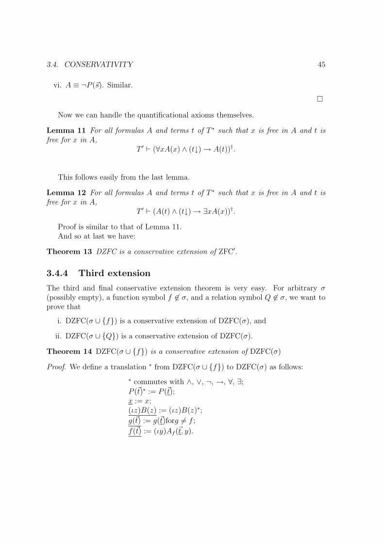
3.4. CONSERVATIVITY 45
vi. A ≡ ¬P (~s). Similar.
¤
Now we can handle the quantificational axioms themselves.
Lemma 11 For all formulas A and terms t of T ∗ such that x is free in A and t isfree for x in A,
T ′ ` (∀xA(x) ∧ (t↓) → A(t))†.
This follows easily from the last lemma.
Lemma 12 For all formulas A and terms t of T ∗ such that x is free in A and t isfree for x in A,
T ′ ` (A(t) ∧ (t↓) → ∃xA(x))†.
Proof is similar to that of Lemma 11.And so at last we have:
Theorem 13 DZFC is a conservative extension of ZFC′.
3.4.4 Third extension
The third and final conservative extension theorem is very easy. For arbitrary σ(possibly empty), a function symbol f 6∈ σ, and a relation symbol Q 6∈ σ, we want toprove that
i. DZFC(σ ∪ f) is a conservative extension of DZFC(σ), and
ii. DZFC(σ ∪ Q) is a conservative extension of DZFC(σ).
Theorem 14 DZFC(σ ∪ f) is a conservative extension of DZFC(σ)
Proof. We define a translation ∗ from DZFC(σ ∪ f) to DZFC(σ) as follows:
∗ commutes with ∧, ∨, ¬, →, ∀, ∃;P (~t)∗ := P (~t);x := x;(ιz)B(z) := (ιz)B(z)∗;g(~t) := g(~t)forg 6= f ;
f(~t) := (ιy)Af (~t, y).
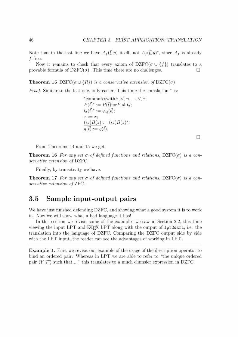
46 CHAPTER 3. FIRST APPLICATION: TRANSLATION
Note that in the last line we have Af (~t, y) itself, not Af (~t, y)∗, since Af is alreadyf -free.
Now it remains to check that every axiom of DZFC(σ ∪ f) translates to aprovable formula of DZFC(σ). This time there are no challenges. ¤
Theorem 15 DZFC(σ ∪ R) is a conservative extension of DZFC(σ)
Proof. Similar to the last one, only easier. This time the translation ∗ is:
∗commuteswith∧,∨,¬,→,∀,∃;P (~t)∗ := P (~t)forP 6= Q;
Q(~t)∗ := ϕQ(~t);x := x;(ιz)B(z) := (ιz)B(z)∗;g(~t) := g(~t).
¤
From Theorems 14 and 15 we get:
Theorem 16 For any set σ of defined functions and relations, DZFC(σ) is a con-servative extension of DZFC.
Finally, by transitivity we have:
Theorem 17 For any set σ of defined functions and relations, DZFC(σ) is a con-servative extension of ZFC.
3.5 Sample input-output pairs
We have just finished defending DZFC, and showing what a good system it is to workin. Now we will show what a bad language it has!
In this section we revisit some of the examples we saw in Section 2.2, this timeviewing the input LPT and LATEX LPT along with the output of lpt2dzfc, i.e. thetranslation into the language of DZFC. Comparing the DZFC output side by sidewith the LPT input, the reader can see the advantages of working in LPT.
Example 1. First we revisit our example of the usage of the description operator tobind an ordered pair. Whereas in LPT we are able to refer to “the unique orderedpair 〈Y, T ′〉 such that...,” this translates to a much clumsier expression in DZFC.
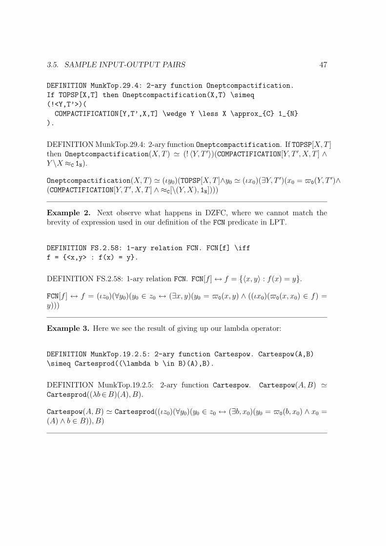
3.5. SAMPLE INPUT-OUTPUT PAIRS 47
DEFINITION MunkTop.29.4: 2-ary function Oneptcompactification.
If TOPSP[X,T] then Oneptcompactification(X,T) \simeq
(!<Y,T’>)(
COMPACTIFICATION[Y,T’,X,T] \wedge Y \less X \approx_C 1_N
).
DEFINITION MunkTop.29.4: 2-ary function Oneptcompactification. If TOPSP[X, T ]then Oneptcompactification(X, T ) ' (! 〈Y, T ′〉)(COMPACTIFICATION[Y, T ′, X, T ] ∧Y \X ≈C 1N).
Oneptcompactification(X, T ) ' (ιy0)(TOPSP[X,T ]∧y0 ' (ιx0)(∃Y, T ′)(x0 = $0(Y, T ′)∧(COMPACTIFICATION[Y, T ′, X, T ] ∧ ≈C[\(Y, X), 1N])))
Example 2. Next observe what happens in DZFC, where we cannot match thebrevity of expression used in our definition of the FCN predicate in LPT.
DEFINITION FS.2.58: 1-ary relation FCN. FCN[f] \iff
f = <x,y> : f(x) = y.
DEFINITION FS.2.58: 1-ary relation FCN. FCN[f ] ↔ f = 〈x, y〉 : f(x) = y.
FCN[f ] ↔ f = (ιz0)(∀y0)(y0 ∈ z0 ↔ (∃x, y)(y0 = $0(x, y) ∧ ((ιx0)($0(x, x0) ∈ f) =y)))
Example 3. Here we see the result of giving up our lambda operator:
DEFINITION MunkTop.19.2.5: 2-ary function Cartespow. Cartespow(A,B)
\simeq Cartesprod((\lambda b \in B)(A),B).
DEFINITION MunkTop.19.2.5: 2-ary function Cartespow. Cartespow(A,B) 'Cartesprod((λb∈B)(A), B).
Cartespow(A,B) ' Cartesprod((ιz0)(∀y0)(y0 ∈ z0 ↔ (∃b, x0)(y0 = $0(b, x0) ∧ x0 =(A) ∧ b ∈ B)), B)

48 CHAPTER 3. FIRST APPLICATION: TRANSLATION
Chapter 4
Second application: Structuralobservations
In this chapter we review various structural data culled from the database of defini-tions in Appendices F and G. In all cases, our data must be understood to reflectnot a necessary logical structure of mathematical concepts, but a historically factualstructure that they have been given, through actual definitions that have been used.
At the same time, different significance must be associated with our differentmeasures: one may be language-dependent, while another may be independent of thelanguage in which the definitions are given. In particular, in the first section belowwe consider a pair of structural measures: the depth and size of each definition’sDAG, or directed acyclic graph of conceptual dependencies. These are independentof the choice of language. On the other hand, in the subsequent section we investigatequantifier depth, which is dependent upon the choice of language.
Which, if any, of our measures are good measures of the complexity of concepts?A good way to answer this would be to scan the definitions in our database, andcompare each against the various structural measures we have investigated. Then,consulting our intuition as to which are the “complex” definitions, we could judgewhich measures gave the best reflection of complexity.
In the sections below we first consider DAGs, then quantifier nesting depth, thenraw symbol count, and finally the types (function or relation, plus arity) of definiendaoccurring in our database.
49

50 CHAPTER 4. SECOND APPLICATION: STRUCTURAL OBSERVATIONS
4.1 Dags
Following Friedman and Flagg in [9], we define the definition DAG (Directed AcyclicGraph) associated to a defined concept α. Intuitively, we begin with the definitiontree for α, and then identify common subtrees to get the DAG.
For the precise definition of a DAG, let Ω be the set of all definienda in ourdatabase. Given α, β ∈ Ω, we say that α depends directly on β, and write
α → β
just in case β appears in the definiens for α.We say that α depends on β, and write
α ⇒ β
if and only if there exists a sequence χ1, . . . , χn ∈ Ω such that
α = χ1 → χ2 → · · · → χn = β.
Then the definition DAG D(α) for a definiendum α, is the graph having as verticesthe set V (D(α)) of all β ∈ Ω such that α ⇒ β, and such that for all β, γ ∈ V (D(α))there is an edge from β to γ just in case β → γ.
We will measure two aspects of each definition DAG. For one, we count the num-ber of vertices appearing in the DAG. We call this the size. We call our secondmeasurement the depth of the DAG, and it is defined to be the greatest n for whichthere is a sequence χ1, . . . , χn ∈ V (D(α)) with
α = χ1 → χ2 → · · · → χn.
We prefer a definition’s DAG to its tree of conceptual dependencies first of allbecause, while the two will have the same depth, the size of the DAG is a more easilyinterpreted measure than the size of the tree. The former tells us how many differentconcepts are involved, whereas the latter is in general a larger number, with a lessobvious meaning.
Secondly, we prefer to develop tools to work with the DAG since it is generally asmaller and much more manageable graph, which is preferable for applications suchas the one discussed in Chapter 5.
We review now some findings on the depths and sizes of the DAGs for the defi-nitions taken from Suppes (Appendix F) and from Munkres (Appendix G). The fulllist of depth and size data can be found in Appendix C.

4.1. DAGS 51
To begin with, consider the histograms for depths and sizes taken across all defi-nitions, from both Suppes and Munkres.
It is interesting to note in the depth histogram that 5 is the most common depth,and that depths 3 through 8 are together very common. The graph has a two-humpedshape. The second hump (depths 22 through 27) corresponds to the Suppes definitionsthat develop the real numbers, as well as the Munkres definitions that mention thereal numbers.
In the size histogram we see that 3 and 7 are the two most common sizes. Thegraph falls off steadily, again with the definitions related to the real numbers respon-sible for the high numbers.
We may also consider the depth and size histograms for the Suppes and Munkresdefinitions separately, as below:

52 CHAPTER 4. SECOND APPLICATION: STRUCTURAL OBSERVATIONS
From these data we can extract the maxima, and the means:
Max MeanAll Depth 32 10.77
Size 110 29.56Suppes Depth 26 10.09
Size 77 25.91Munkres Depth 32 12.25
Size 110 36.01
Note that DAG measurements such as depth and size are reflections not of thelanguage in which we have chosen to write our definitions, but only of the definitionalstructure we have chosen.
Something that we see reflected in the depth numbers for the Munkres definitions(in Appendix C), is that any definition involving mention of the real numbers isinordinately deep. Consider for example the definition of the standard topology onthe reals, in Chapter 13 (Stdrealtop:0), which has depth 24.
This depth reflects all the work that goes into formally defining the reals. To astudent, on the other hand, this depth has nothing to do with the difficulty of theconcept; to the student, the real numbers bring in no conceptual difficulty whatso-ever. Quite the contrary, their involvement is a conceptual aid, in that it allows theproduction of a concrete example.
4.2 Quantifier depths
In this section we examine the quantifier depths occurring in the definitions in ourdatabase. Quantifier depth can be regarded in two different ways. Consider the

4.2. QUANTIFIER DEPTHS 53
following example:
DEFINITION MunkTop.21.3: 7-ary relation UNIFCONV. If TOPSP[X,T ]∧METRICSPACE[Y, T ′, d] ∧ FCN[F ] ∧ Dom(F ) = N∧(∀n∈N)(FCN[F (n), X, Y ]) thenUNIFCONV[F, f, X, T, Y, T ′, d] ↔ (∀ε∈R)(ε>R 0R → (∃N ∈N)((∀n>N N)(∀x∈X)(d(F (n)(x), f(x)) <R ε))).
The <R relation occurs inside of a universal quantifier, followed by an existentialquantifier, and then two universal quantifiers. Counting only quantifier alternations,we would say then that the <R relation occurs at depth 3. If on the other hand wecount any and all quantifiers, whether or not they alternate, then the <R relationoccurs at depth 4.
Alternating depth is typically of greater interest as logical structure is concerned.Consider for example the arithmetic hierarchy. I believe however that non-alternatingdepth is also of interest, at least psychologically. The two subsequent universal quan-tifiers in the example above introduce two different kinds of things that the readermust keep track of: a natural number greater than N , and an element of the set X.This is more complex than what would be introduced by a single quantifier.
We will measure both alternating, and non-alternating, quantifier depth for eachdefinition. In addition, we will regard each definition at three different levels ofexpansion.
To expand a definition is to replace each defined function or relation appearing inthe definiens by its own definiens. This process may be repeated recursively until ithalts. In this case we will say that the given definition was expanded fully.
In general, let Ω be the set of all definienda in our database. Given α ∈ Ω, anda set B = β1, . . . , βn ⊆ Ω, we define the expansion of α relative to B, which wedenote E (α,B), to be what we get by replacing all definienda in α, except those inB, by their definiens; and repeating this process until it halts.
Altogether, in this section we consider for each definition α in our database, eightdata points: Both alternating, and non-alternating, quantifier depth, for α viewed asgiven in LPT; as translated into DZFC; and then as the translation into DZFC isboth fully expanded, and expanded relative to the set of the following foundationaldefinitions:
DEFINITION builtIn1: Infix function ∪. x∪ y ' z : z ∈x ∨ z ∈ y. Precedence 40.
DEFINITION builtIn2: Infix function ∩. x∩ y ' z : z ∈x ∧ z ∈ y. Precedence 30.
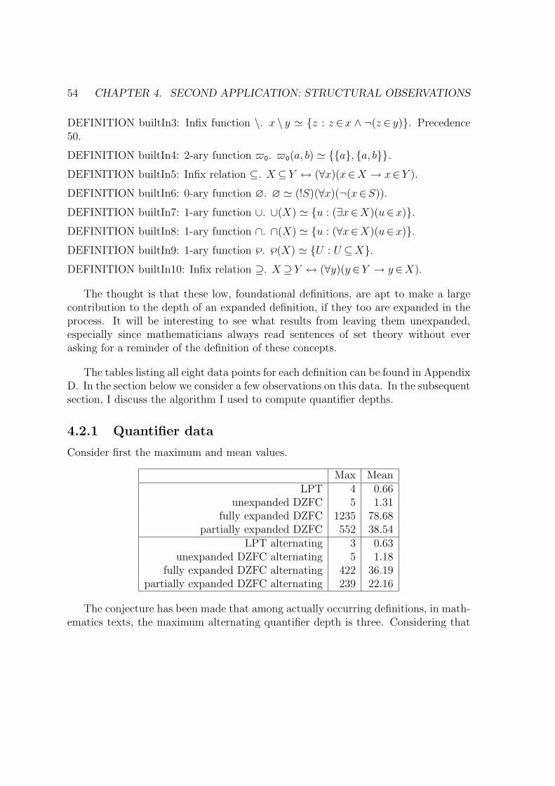
54 CHAPTER 4. SECOND APPLICATION: STRUCTURAL OBSERVATIONS
DEFINITION builtIn3: Infix function \. x \ y ' z : z ∈x ∧ ¬(z ∈ y). Precedence50.
DEFINITION builtIn4: 2-ary function $0. $0(a, b) ' a, a, b.DEFINITION builtIn5: Infix relation ⊆. X ⊆Y ↔ (∀x)(x∈X → x∈Y ).
DEFINITION builtIn6: 0-ary function ∅. ∅ ' (!S)(∀x)(¬(x∈S)).
DEFINITION builtIn7: 1-ary function ∪. ∪(X) ' u : (∃x∈X)(u∈x).DEFINITION builtIn8: 1-ary function ∩. ∩(X) ' u : (∀x∈X)(u∈x).DEFINITION builtIn9: 1-ary function ℘. ℘(X) ' U : U ⊆X.DEFINITION builtIn10: Infix relation ⊇. X ⊇Y ↔ (∀y)(y ∈Y → y ∈X).
The thought is that these low, foundational definitions, are apt to make a largecontribution to the depth of an expanded definition, if they too are expanded in theprocess. It will be interesting to see what results from leaving them unexpanded,especially since mathematicians always read sentences of set theory without everasking for a reminder of the definition of these concepts.
The tables listing all eight data points for each definition can be found in AppendixD. In the section below we consider a few observations on this data. In the subsequentsection, I discuss the algorithm I used to compute quantifier depths.
4.2.1 Quantifier data
Consider first the maximum and mean values.
Max MeanLPT 4 0.66
unexpanded DZFC 5 1.31fully expanded DZFC 1235 78.68
partially expanded DZFC 552 38.54LPT alternating 3 0.63
unexpanded DZFC alternating 5 1.18fully expanded DZFC alternating 422 36.19
partially expanded DZFC alternating 239 22.16
The conjecture has been made that among actually occurring definitions, in math-ematics texts, the maximum alternating quantifier depth is three. Considering that
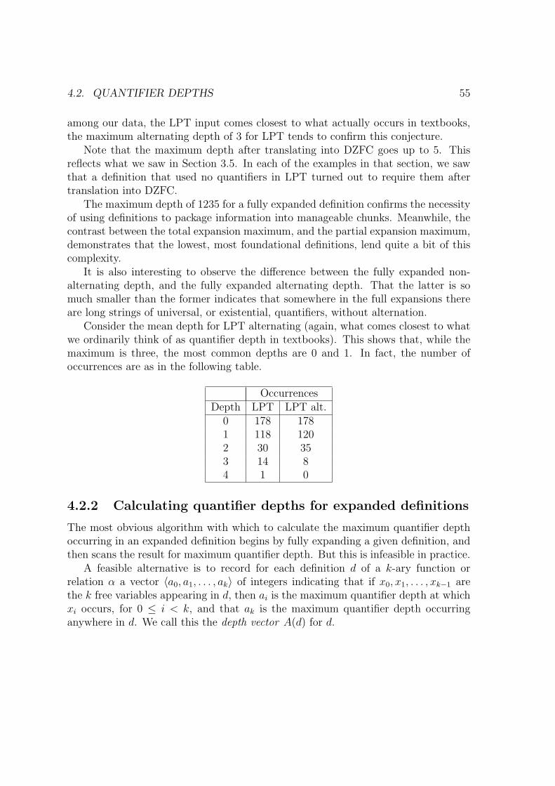
4.2. QUANTIFIER DEPTHS 55
among our data, the LPT input comes closest to what actually occurs in textbooks,the maximum alternating depth of 3 for LPT tends to confirm this conjecture.
Note that the maximum depth after translating into DZFC goes up to 5. Thisreflects what we saw in Section 3.5. In each of the examples in that section, we sawthat a definition that used no quantifiers in LPT turned out to require them aftertranslation into DZFC.
The maximum depth of 1235 for a fully expanded definition confirms the necessityof using definitions to package information into manageable chunks. Meanwhile, thecontrast between the total expansion maximum, and the partial expansion maximum,demonstrates that the lowest, most foundational definitions, lend quite a bit of thiscomplexity.
It is also interesting to observe the difference between the fully expanded non-alternating depth, and the fully expanded alternating depth. That the latter is somuch smaller than the former indicates that somewhere in the full expansions thereare long strings of universal, or existential, quantifiers, without alternation.
Consider the mean depth for LPT alternating (again, what comes closest to whatwe ordinarily think of as quantifier depth in textbooks). This shows that, while themaximum is three, the most common depths are 0 and 1. In fact, the number ofoccurrences are as in the following table.
OccurrencesDepth LPT LPT alt.
0 178 1781 118 1202 30 353 14 84 1 0
4.2.2 Calculating quantifier depths for expanded definitions
The most obvious algorithm with which to calculate the maximum quantifier depthoccurring in an expanded definition begins by fully expanding a given definition, andthen scans the result for maximum quantifier depth. But this is infeasible in practice.
A feasible alternative is to record for each definition d of a k-ary function orrelation α a vector 〈a0, a1, . . . , ak〉 of integers indicating that if x0, x1, . . . , xk−1 arethe k free variables appearing in d, then ai is the maximum quantifier depth at whichxi occurs, for 0 ≤ i < k, and that ak is the maximum quantifier depth occurringanywhere in d. We call this the depth vector A(d) for d.

56 CHAPTER 4. SECOND APPLICATION: STRUCTURAL OBSERVATIONS
Then we may compute the quantifier depth of d as a function of the depths of thek arguments. We define the function
D(d)(x0, . . . , xk−1) := max(a0 + x0, . . . , ak−1 + xk−1, ak).
Then if the quantifier depths of the k arguments are b0, . . . , bk−1, then the depth of dwhen we plug in these arguments is D(d)(b0, . . . , bk−1).
Now suppose d0, d1, . . . , dn are the definitions for which we wish to compute thequantifier depth. Assume that d0 has no conceptual dependencies (its DAG hasdepth 1), and that for i > 0 the set of concepts on which di depends is containedin d0, . . . , di−1. Then we may proceed by first computing the depth vector A(d0)for d0 and storing it. Then we return D(d0)(0, . . . , 0), the maximum quantifier depthoccurring in d0.
We then proceed similarly for the remaining di, consulting our stored depth vectorswhenever we encounter a defined function or relation. With this algorithm we canfeasibly compute the quantifier depths for all of the definitions in our database.
A slightly modified algorithm is needed in order to compute the alternating quan-tifier depths. The basic process is the same, only the depth vectors need to containmore information. This time, if the defined function or relation is k-ary, then, insteadof a vector of length k + 1, we will store a vector of length 4k + 2, the entries beingas follows:
i. For each of the k free variables, xi, we record the maximum number of alter-nating nested quantifiers under which xi occurs, such that:
(i) the first quantifier is ∃ and the last is also ∃,(ii) the first is ∃ and the last is ∀,(iii) the first is ∀ and the last is ∃,(iv) the first is ∀ and the last is also ∀.
ii. We record the maximum depth of quantifiers occurring anywhere in the defini-tion and starting with ∃
iii. We record the maximum depth of quantifiers occurring anywhere in the defini-tion and starting with ∀.
We must then follow a somewhat more complex process in order to use these depthvectors, but otherwise the algorithm is essentially the same as in the non-alternatingcase.
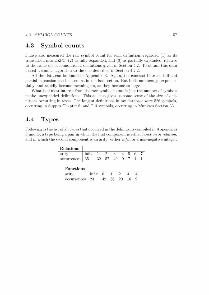
4.3. SYMBOL COUNTS 57
4.3 Symbol counts
I have also measured the raw symbol count for each definition, regarded (1) as itstranslation into DZFC; (2) as fully expanded; and (3) as partially expanded, relativeto the same set of foundational definitions given in Section 4.2. To obtain this dataI used a similar algorithm to the one described in Section 4.2.2.
All the data can be found in Appendix E. Again, the contrast between full andpartial expansion can be seen, as in the last section. But both numbers go exponen-tially, and rapidly become meaningless, as they become so large.
What is of most interest from the raw symbol counts is just the number of symbolsin the unexpanded definitions. This at least gives us some sense of the size of defi-nitions occurring in texts. The longest definitions in my database were 526 symbols,occurring in Suppes Chapter 6; and 714 symbols, occurring in Munkres Section 33.
4.4 Types
Following is the list of all types that occurred in the definitions compiled in AppendicesF and G, a type being a pair in which the first component is either function or relation;and in which the second component is an arity: either infix, or a non-negative integer.
Relationsarity infix 1 2 3 4 5 6 7occurrences 35 32 57 40 9 7 1 1
Functionsarity infix 0 1 2 3 4occurrences 23 42 36 20 16 9

58 CHAPTER 4. SECOND APPLICATION: STRUCTURAL OBSERVATIONS

Chapter 5
Third application: Knowledgegraphs
To a student exploring a new field of mathematics, the defined concepts of the fieldrepresent a first hurdle that must be cleared. The language cannot even be understooduntil the concepts are. For a dedicated student beginning to study a well-definedsubject, a traditional approach using a textbook may be best. But it is difficult tolook ahead in a textbook, to get a quick view of what is to come. A student wishingto look ahead, or even an expert from another field dabbling in a foreign subject, willbenefit from software that allows the quick diagrammatic representation of conceptualdependencies.
Suppose for example that someone knowing nothing about modularity theorywants to understand the concepts involved in the proof of Fermat’s Last Theorem.They will locate a book on elliptic curves, and attempt to find out what it means foran elliptic curve to be modular. They will find the definitions of these concepts inthe book, and discover that these depend on prior concepts, also unknown. And so abackwards chase through the book is initiated.
My program, kmap (for “knowledge map”), addresses the needs of such a student.In the first section below, I go over its usage. In the following section I discuss futureimprovements.
5.1 kmap
The user of kmap begins by typing in the name and arity of the definition D to beexplored, and pressing Enter.
59

60 CHAPTER 5. THIRD APPLICATION: KNOWLEDGE GRAPHS
This causes the root node of the definition DAG for D to be displayed in theGraphViewer window.
The user then has the option to click on nodes in the GraphViewer window, andchoose either to “expand” or “collapse” them.
Expanding a node causes all of the concepts on which it directly depends (i.e. allthose concepts mentioned explicitly in its definiens) to be displayed beneath it, withdirected edges drawn in to show the dependencies.

5.1. KMAP 61
Collapsing a node deletes all nodes that are depended upon only by it.
By clicking and dragging with the mouse, the user can rearrange the nodes of thegraph.
Since many of the concepts arising in the expansion process will be well-known,and therefore boring, to a student, my program also offers the option to “sideline” aconcept.
For example, in the figure above, the lowest node displays our name for the orderedpair function. This can be sidelined, in order to remove clutter from the diagram.The user right-clicks on the node, and selects “Sideline”.

62 CHAPTER 5. THIRD APPLICATION: KNOWLEDGE GRAPHS
This causes the node to be relocated to the left-hand margin of the GraphViewerwindow, and all edges connecting the node to the rest of the graph to be (temporarily)deleted.
The user is free to “unsideline” any sidelined concepts at any time, returning themto their prior location within the graph.
5.2 Future directions
Names. The sorts of names we have used for the definitions in Appendix G aresomewhat difficult to read. After some time away from them, a user could forgetwhat they abbreviate.

5.2. FUTURE DIRECTIONS 63
A better alternative is to work within various namespaces, so that what is ex-traneous or hard to read can be removed from the names. For example, if it wasknown that we were working in the Topology context, then we could simply defineconvergent, rather TOPCONV.
Generally, within a program like kmap, it would be an improvement to see morereadable tags on the vertices. Instead of the sort of highly abbreviated names wehave used here, it would be good to see a more complete description of the conceptbeing referenced.
Other vertex types. As we explore the DAGs for defined concepts, while keeping inmind the goal of developing software that will allow a student to explore a new areaof mathematics, it becomes apparent what is missing. In addition to concepts, theKnowledge Map environment should also allow us to explore the network of theoremsand proofs that make up a theory. (To incorporate proofs we would have to choose alanguage in which to represent them, which LPT does not provide.)
Ultimately we should have Knowledge Maps that feature three kinds of vertices,corresponding to theorems, proofs, and concepts. The edges would be as follows:
1. Theorem → Proof. This indicates that the proof is a proof of this theorem.
2. Theorem → Concept. This indicates that the concept is mentioned in thestatement of the theorem.
3. Proof → Theorem. The theorem is cited in the course of the proof.
4. Proof → Concept. The concept is used in the course of the proof.
5. Concept → Concept. This is the sort of edge we have already considered inour definition DAGs, indicating that the first concept is defined in terms of thesecond one.
Edges of types 2 and 5 in the list above could be computed by a parsing program,as has been done in my program. Edges of type 1 would perhaps represent datainput by hand, or else could follow from the name of the proof, if appropriate namingconventions were set up. Edges of types 3 and 4 would, I believe, have to be inputby hand, and in fact this would require mathematical expertise.
64 CHAPTER 5. THIRD APPLICATION: KNOWLEDGE GRAPHS

Appendix A
Characters and Strings in LPT
A.1 Characters
LPT features a large character set, which we divide into several subsets as follows.
1. English letters: Capital and lowercase, from A to z. These characters may beentered inside of any of the following LATEX font commands:
\mathbf \mathcal \mathfrak \mathscr \mathbb
2. Greek letters: Capital and lowercase, from Γ to ω (except λ, π, and ω, whichare reserved for other purposes), plus the usual LATEX variations: ε, ϑ, $, %, ς,ϕ.
α \alpha β \beta γ \gamma δ \deltaε \epsilon ε \varepsilon ζ \zeta η \etaθ \theta ϑ \vartheta ι \iota κ \kappaµ \mu ν \nu ξ \xi$ \varpi ρ \rho % \varrho σ \sigmaς \varsigma τ \tau υ \upsilon φ \phiϕ \varphi χ \chi ψ \psi Γ \Gamma∆ \Delta Θ \Theta Λ \Lambda Ξ \XiΠ \Pi Σ \Sigma Υ \Upsilon Φ \PhiΨ \Psi Ω \Omega
3. Digits: 0, 1, 2, 3, 4, 5, 6, 7, 8, 9.
65

66 APPENDIX A. CHARACTERS AND STRINGS IN LPT
4. Function characters: Here we include many of the popular function symbols inAMS LATEX.
π \pi ω \omega + + \ \less/ / | | ∪ \cup ∩ \capt \sqcup u \sqcap ⊕ \oplus ⊗ \otimes× \times ÷ \div \circ · \cdot∅ \varnothing ∞ \infty ℘ \wp ∑ \sum∏ \prod ∐ \coprod ⋃ \bigcup ⋂ \bigcap⊔ \bigsqcup ∨ \bigvee ∧ \bigwedge ⊗ \bigotimes⊕ \bigoplus ℵ \aleph i \beth ג \gimelk \daleth < \Re = \Im ∂ \partial∇ \nabla
5. Relation characters: Likewise, we include many of the popular relation symbolsin AMS LATEX.
≤ \leq ≥ \geq ≺ \prec  \succ¹ \preceq º \succeq ¿ \ll À \gg⊂ \subset ⊃ \supset ⊆ \subseteq ⊇ \supseteqv \sqsubseteq w \sqsupseteq ∈ \in ` \vdasha \dashv ≡ \equiv |= \models ∼ \sim⊥ \perp | \mid ³ \asymp ‖ \parallel≈ \approx ^ \smile ∼= \cong _ \frown∝ \propto .
= \doteq ./ \bowtie C \lhdB \rhd E \unlhd D \unrhd
6. Decorating characters: The usual LATEX decorations, plus primes and asterisks.
a \hata a \tildea a \bara ~a \vecaa \dota a′ a’ a∗ a^*
7. Reserved characters: The logical connectives and quantifiers, =, 6=, braces,brackets, etc. The Greek letter λ is reserved for lambda abstraction.
∧ \wedge ∨ \vee → \implies ¬ \neg∀ \forall ∃ \exists > \top ⊥ \bot↔ \iff = 6= \neq ' \simeq↑ \up ↓ \dn < >[ ] ( ) λ \lambda !
A.2. STRINGS 67
A.2 Strings
Here we describe the formation of the strings to be used in LPT for the naming ofdefined functions and relations, as well as variables.
Function strings: A function string consists of
i. Two or more English letters, the first of which is capital and the rest of whichare lowercase, or
ii. A function symbol, or
iii. A numeral, or
iv. A Greek letter
followed by an optional subscript and/or primes or an asterisk. The subscript isentered with an underscore and braces as in LATEX, and may contain any stringof characters in the language. In cases (iii) and (iv) there must be a subscript ordecorating character.
Examples: Stonecech, +, t, 0Nat.
Relation strings: A relation string consists of
i. Two or more English letters, all of which are capital, or
ii. A relation symbol
followed by an optional subscript and/or primes or an asterisk.
Examples: GROUP, ∈, <Nat.
Variable strings: A variable string consists of
i. An English letter in any font, or
ii. A Greek letter,
where the letter is given any of the five LATEX decorations mentioned in point vi above,as well as zero or more primes, an optional asterisk, and/or an optional subscriptconsisting of a nonnegative numeral.

68 APPENDIX A. CHARACTERS AND STRINGS IN LPT

Appendix B
Our LPT grammar is not LL
Let G be the grammar for LPT implemented by our parsing program, as compiledby ACCENT. Using the techniques and notations of [3], we prove that G is not LL.
In the first section below, we give the proof. In the subsequent section we presentthe entire grammar for LPT, as passed to our compiler compiler, ACCENT.
B.1 Proof
We begin by introducing abbreviations for the following nonterminals and terminalsof G . (See the next section for the entire grammar.)
Nonterminalsabbreviation nonterminal abbreviation nonterminal
S def list A definition
B defname C defbody
D numeral E rstr
F relndef G relndefunit
H varseq I formula
J var K bformula
L termformula M term
Q bterm R aterm
69

70 APPENDIX B. OUR LPT GRAMMAR IS NOT LL
Terminalsabbreviation terminal
a DEFINITION
b ARY
c RELN
d RELNSYM
e IFF
f LETTER
g TOP
h UPARROW
The nonterminal S is the start symbol of the grammar.Apart from the terminals listed above, we also have:
0 . ( ) [ ]
Given these abbreviations, the following productions (among many others) belongto the grammar:
S → A E → d J → f M → QA → aBC F → G. K → (I) Q → RB → 0 G → E[H]eI K → g R → (M)C → DbcE.F H → J K → L R → DD → 0 I → K L → Mh
Now let an arbitrary non-negative integer k be given. It is easy to see that with
w = a00bcd.d[f ]e
α = .
β = (I)
γ = L
x = ((· · · (︸ ︷︷ ︸k
we have
S∗⇒
lmxKα
K → β and K → γ
x ∈ FIRSTk(βα) ∩ FIRSTk(γα)
whence it follows, from Theorem 5.2 of [3], that G is not LL(k). Since k was arbitrary,G is not LL.

B.2. THE GRAMMAR 71
B.2 The grammar
We reproduce the source code sent to ACCENT, from which it produced an Earleyalgorithm parser for LPT. The reader may consult [14] regarding the syntax for AC-CENT. Briefly, the source code begins with a list of the tokens of the language, whichstand for terminal symbols, in all capitals at the beginning. (Other, single-characterterminal symbols can be used without a token to represent them.) Thereafter we havea paragraph for each nonterminal, in which its productions are given in Backus-Naurform.
%prelude
#include "yystype.h"
#include "stdio.h"
FILE *pFile;
char AST[10000];
char UP[] = "$<";
char DN[] = "$>";
%token ALLCAPS, ARY, BOT, DECORATION,
DEFINITION, DIGITS, DOWN, EXISTS, FIXED, FONT,
FORALL, FUNC, FUNCSYM, GENWORD, GREEK,
IF, IFF, INFIX, INFIXFN, INFIXRL, INITCAP,
LAMBDA, LETTER, LETTERS, MATHBB, MISCLETTER,
NEG, NEQ, NZNUM, OTHERWISE, PRECEDENCE,
RELN, RELNSYM, SIMEQ, THEN, THENSYM, TOP,
UPARROW, VEE, WEDGE;
// -------------------- TRUNK --------------------------
def_list :
pFile = fopen("lptout","w");
definition fprintf(pFile, "%s", AST); strcpy(AST,"");
( strcat(AST,"\n\n");
definition fprintf(pFile, "%s", AST); strcpy(AST,"");
)*
fclose(pFile);

72 APPENDIX B. OUR LPT GRAMMAR IS NOT LL
;
// ------------------------------------------------------
definition :
%prelude strcat(AST,DN); strcat(AST,"definition");
DEFINITION defname (defbody|infixdefbody)
strcat(AST,UP);
;
// ------------------------------------------------------
defname :
//Definition names are made from alphanumeric characters,
//as well as the period and underscore characters.
%prelude strcat(AST,DN); strcat(AST,"defname");
strcat(AST,"$$");
( ’0’ strcat(AST,"0");
| ’_’ strcat(AST,"_");
| NZNUM<s> strcat(AST,s);
| DIGITS<s> strcat(AST,s);
| LETTER<s> strcat(AST,s);
| INITCAP<s> strcat(AST,s);
| ALLCAPS<s> strcat(AST,s);
| LETTERS<s> strcat(AST,s);
| GENWORD<s> strcat(AST,s);
| ’.’ strcat(AST,".");
)
( ’0’ strcat(AST,"0");
| ’_’ strcat(AST,"_");
| NZNUM<s> strcat(AST,s);
| DIGITS<s> strcat(AST,s);
| LETTER<s> strcat(AST,s);
| INITCAP<s> strcat(AST,s);
| ALLCAPS<s> strcat(AST,s);
| LETTERS<s> strcat(AST,s);
| GENWORD<s> strcat(AST,s);
| ’.’ strcat(AST,".");
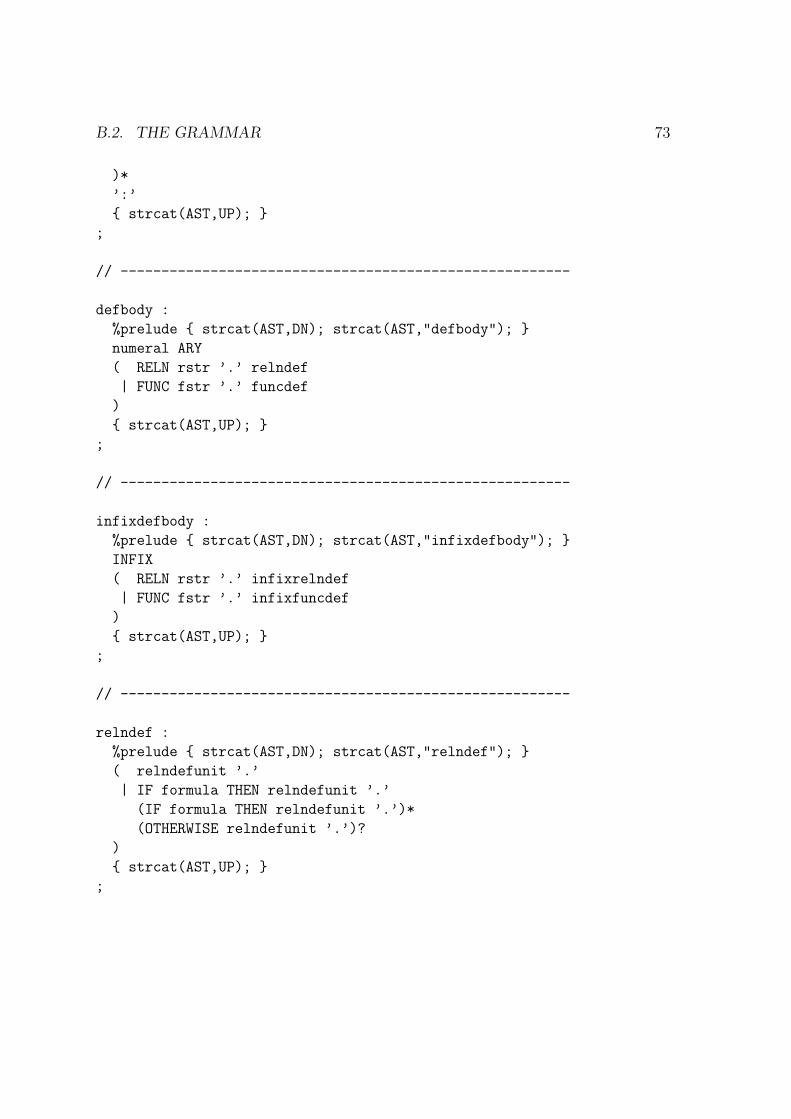
B.2. THE GRAMMAR 73
)*
’:’
strcat(AST,UP);
;
// -------------------------------------------------------
defbody :
%prelude strcat(AST,DN); strcat(AST,"defbody");
numeral ARY
( RELN rstr ’.’ relndef
| FUNC fstr ’.’ funcdef
)
strcat(AST,UP);
;
// -------------------------------------------------------
infixdefbody :
%prelude strcat(AST,DN); strcat(AST,"infixdefbody");
INFIX
( RELN rstr ’.’ infixrelndef
| FUNC fstr ’.’ infixfuncdef
)
strcat(AST,UP);
;
// -------------------------------------------------------
relndef :
%prelude strcat(AST,DN); strcat(AST,"relndef");
( relndefunit ’.’
| IF formula THEN relndefunit ’.’
(IF formula THEN relndefunit ’.’)*
(OTHERWISE relndefunit ’.’)?
)
strcat(AST,UP);
;

74 APPENDIX B. OUR LPT GRAMMAR IS NOT LL
// -------------------------------------------------------
relndefunit :
%prelude strcat(AST,DN); strcat(AST,"relndefunit");
rstr ’[’ varseq ’]’ IFF formula
strcat(AST,UP);
;
// -------------------------------------------------------
infixrelndef :
%prelude strcat(AST,DN); strcat(AST,"infixrelndef");
( infixrelndefunit ’.’
| IF formula THEN infixrelndefunit ’.’
(IF formula THEN infixrelndefunit ’.’)*
(OTHERWISE infixrelndefunit ’.’)?
)
strcat(AST,UP);
;
// -------------------------------------------------------
infixrelndefunit :
%prelude strcat(AST,DN); strcat(AST,"infixrelndefunit");
var rstr var IFF formula
strcat(AST,UP);
;
// -------------------------------------------------------
funcdef :
%prelude strcat(AST,DN); strcat(AST,"funcdef");
( funcdefunit ’.’
| IF formula THEN funcdefunit ’.’
(IF formula THEN funcdefunit ’.’)*
(OTHERWISE funcdefunit ’.’)?
)

B.2. THE GRAMMAR 75
strcat(AST,UP);
;
// -------------------------------------------------------
funcdefunit :
%prelude strcat(AST,DN); strcat(AST,"funcdefunit");
composite (SIMEQ term | UPARROW)
strcat(AST,UP);
;
// -------------------------------------------------------
infixfuncdef :
%prelude strcat(AST,DN); strcat(AST,"infixfuncdef");
( infixfuncdefunit ’.’ precedence ’.’
| IF formula THEN infixfuncdefunit ’.’
(IF formula THEN infixfuncdefunit ’.’)*
(OTHERWISE infixfuncdefunit ’.’)? precedence ’.’
)
strcat(AST,UP);
;
// -------------------------------------------------------
infixfuncdefunit :
%prelude strcat(AST,DN); strcat(AST,"infixfuncdefunit");
var fstr var (SIMEQ term | UPARROW)
strcat(AST,UP);
;
// -------------------------------------------------------
precedence :
%prelude strcat(AST,DN); strcat(AST,"precedence");
strcat(AST,"$$");
PRECEDENCE (’-’ strcat(AST,"-");)?
( ’0’ strcat(AST,"0");

76 APPENDIX B. OUR LPT GRAMMAR IS NOT LL
| NZNUM<s> strcat(AST,s);
| DIGITS<s> strcat(AST,s);
)
strcat(AST,UP);
;
// ---------------------- BRANCHES -----------------------
term :
%prelude strcat(AST,DN); strcat(AST,"term");
bterm (infixfunc bterm)*
strcat(AST,UP);
;
// -------------------------------------------------------
bterm :
%prelude strcat(AST,DN); strcat(AST,"bterm");
aterm (evaluation)*
strcat(AST,UP);
;
// -------------------------------------------------------
aterm :
%prelude strcat(AST,DN); strcat(AST,"aterm");
( var
| numeral
| composite
| ’(’ term ’)’
| set
| tuple
| unique
| lambda
)
strcat(AST,UP);
;

B.2. THE GRAMMAR 77
// -------------------------------------------------------
varseq :
%prelude strcat(AST,DN); strcat(AST,"varseq");
var (’,’ var)*
strcat(AST,UP);
;
// -------------------------------------------------------
composite :
%prelude strcat(AST,DN); strcat(AST,"composite");
fstr (evaluation)?
strcat(AST,UP);
;
// -------------------------------------------------------
set :
%prelude strcat(AST,DN); strcat(AST,"set");
’’ term ( (’,’ termseq)? strcat(AST,"$$"); ’’
| (infixrel termseq)? ’:’ formula ( ’’
| ’,’ varseq FIXED ’’
)
)
strcat(AST,UP);
;
// -------------------------------------------------------
tuple :
%prelude strcat(AST,DN); strcat(AST,"tuple");
’<’ termseq ’>’
strcat(AST,UP);
;
// -------------------------------------------------------
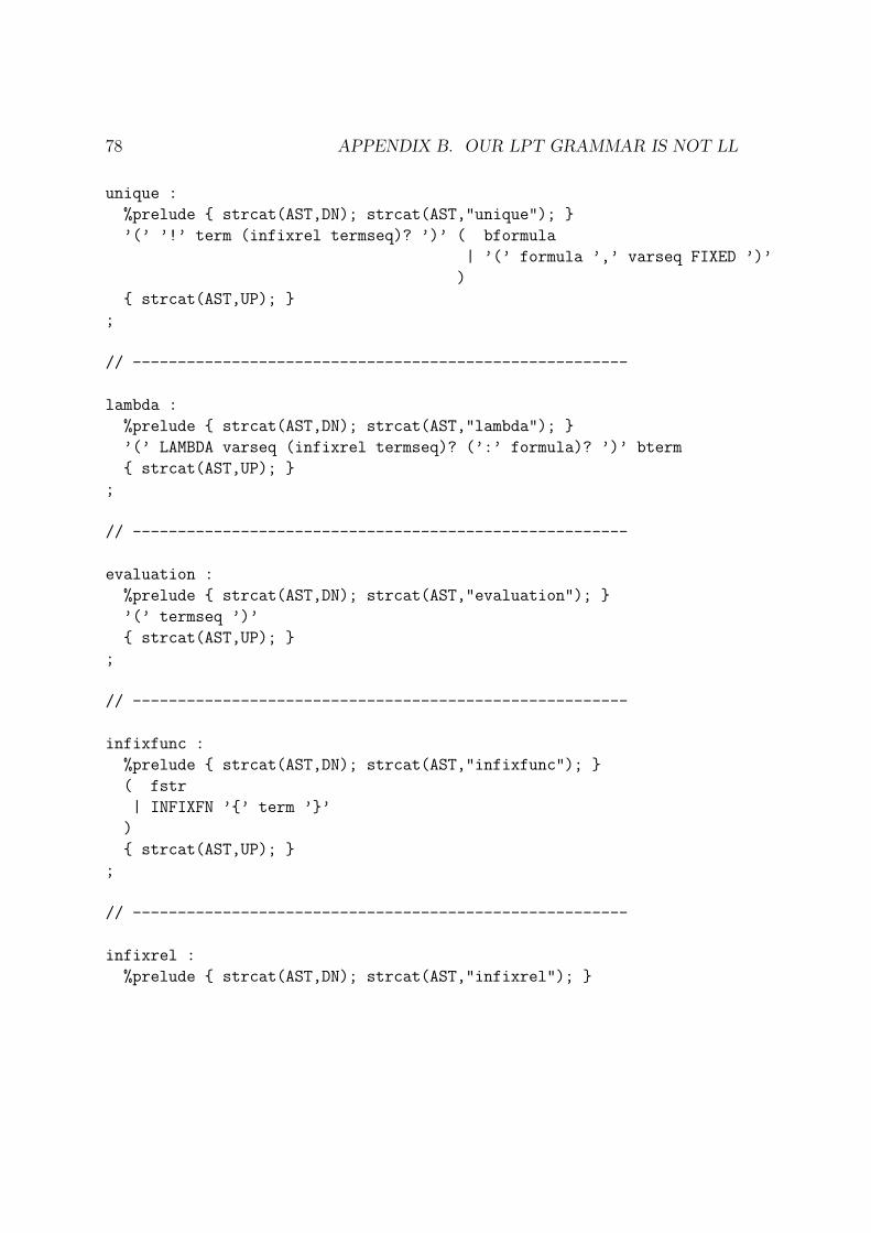
78 APPENDIX B. OUR LPT GRAMMAR IS NOT LL
unique :
%prelude strcat(AST,DN); strcat(AST,"unique");
’(’ ’!’ term (infixrel termseq)? ’)’ ( bformula
| ’(’ formula ’,’ varseq FIXED ’)’
)
strcat(AST,UP);
;
// -------------------------------------------------------
lambda :
%prelude strcat(AST,DN); strcat(AST,"lambda");
’(’ LAMBDA varseq (infixrel termseq)? (’:’ formula)? ’)’ bterm
strcat(AST,UP);
;
// -------------------------------------------------------
evaluation :
%prelude strcat(AST,DN); strcat(AST,"evaluation");
’(’ termseq ’)’
strcat(AST,UP);
;
// -------------------------------------------------------
infixfunc :
%prelude strcat(AST,DN); strcat(AST,"infixfunc");
( fstr
| INFIXFN ’’ term ’’
)
strcat(AST,UP);
;
// -------------------------------------------------------
infixrel :
%prelude strcat(AST,DN); strcat(AST,"infixrel");

B.2. THE GRAMMAR 79
( rstr
| ’=’ strcat(AST,"$$=");
| NEQ strcat(AST,"$$\\neq");
| SIMEQ strcat(AST,"$$\\simeq");
| INFIXRL ’’ term ’’
)
strcat(AST,UP);
;
// -------------------------------------------------------
termseq :
%prelude strcat(AST,DN); strcat(AST,"termseq");
term (’,’ term)*
strcat(AST,UP);
;
// -------------------------------------------------------
formula :
%prelude strcat(AST,DN); strcat(AST,"formula");
bformula (lc bformula)*
strcat(AST,UP);
;
// -------------------------------------------------------
lc :
%prelude strcat(AST,DN); strcat(AST,"lc");
strcat(AST,"$$");
( VEE strcat(AST,"\\vee");
| WEDGE strcat(AST,"\\wedge");
| THENSYM strcat(AST,"\\rightarrow");
| IFF strcat(AST,"\\rightleftarrow");
)
strcat(AST,UP);
;

80 APPENDIX B. OUR LPT GRAMMAR IS NOT LL
// -------------------------------------------------------
bformula :
%prelude strcat(AST,DN); strcat(AST,"bformula");
( BOT strcat(AST,"$$\\bot");
| TOP strcat(AST,"$$\\top");
| termformula
| relation
| ’(’ formula ’)’
| negation
| onetrue
| forall
| exists
| existsunique
)
strcat(AST,UP);
;
// -------------------------------------------------------
termformula :
%prelude strcat(AST,DN); strcat(AST,"termformula");
term ( UPARROW strcat(AST,"$$\\uparrow");
| DOWN strcat(AST,"$$\\downarrow");
| strcat(AST,"$$"); ’[’ termseq ’]’
| (’,’ termseq)? infixrel termseq (infixrel termseq)*
)
strcat(AST,UP);
;
// -------------------------------------------------------
relation :
%prelude strcat(AST,DN); strcat(AST,"relation");
rstr ’[’ termseq ’]’
strcat(AST,UP);
;

B.2. THE GRAMMAR 81
// -------------------------------------------------------
negation :
%prelude strcat(AST,DN); strcat(AST,"negation");
NEG bformula
strcat(AST,UP);
;
// -------------------------------------------------------
onetrue :
%prelude strcat(AST,DN); strcat(AST,"onetrue");
’!’ ’[’ formulaseq ’]’
strcat(AST,UP);
;
// -------------------------------------------------------
formulaseq :
%prelude strcat(AST,DN); strcat(AST,"formulaseq");
formula (’,’ formula)*
strcat(AST,UP);
;
// -------------------------------------------------------
forall :
%prelude strcat(AST,DN); strcat(AST,"forall");
’(’ FORALL termseq
( ’:’ strcat(AST,"$$"); formula ’)’ bformula
| (infixrel termseq)? ’)’
( bformula
| ’(’ formula ’,’ varseq FIXED ’)’
)
)
strcat(AST,UP);
;

82 APPENDIX B. OUR LPT GRAMMAR IS NOT LL
// -------------------------------------------------------
exists :
%prelude strcat(AST,DN); strcat(AST,"exists");
’(’ EXISTS termseq
( ’:’ strcat(AST,"$$"); formula ’)’ bformula
| (infixrel termseq)? ’)’
( bformula
| ’(’ formula ’,’ varseq FIXED ’)’
)
)
strcat(AST,UP);
;
// -------------------------------------------------------
existsunique :
%prelude strcat(AST,DN); strcat(AST,"existsunique");
’(’ EXISTS ’!’ termseq
( ’:’ strcat(AST,"$$"); formula ’)’ bformula
| (infixrel termseq)? ’)’
( bformula
| ’(’ formula ’,’ varseq FIXED ’)’
)
)
strcat(AST,UP);
;
// --------------------- LEAVES -------------------------
var :
%prelude strcat(AST,DN); strcat(AST,"var");
strcat(AST,"$$");
(DECORATION<s> strcat(AST,s); )?
( FONT<s> strcat(AST,s);
’’ strcat(AST,"");
LETTER<s> strcat(AST,s);
’’ strcat(AST,"");

B.2. THE GRAMMAR 83
| LETTER<s> strcat(AST,s);
| MISCLETTER<s> strcat(AST,s);
| GREEK<s> strcat(AST,s);
)
(’’’ strcat(AST,"’"); )*
( ’_’ ’’ strcat(AST,"_");
( ’0’ strcat(AST,"0");
| NZNUM<s> strcat(AST,s);
| DIGITS<s> strcat(AST,s);
)
’’ strcat(AST,"");
(’*’ strcat(AST,"^*"); )?
| ’*’ strcat(AST,"^*");
(’_’ ’’ strcat(AST,"_");
( ’0’ strcat(AST,"0");
| NZNUM<s> strcat(AST,s);
| DIGITS<s> strcat(AST,s);
)
’’ strcat(AST,"");
)?
)?
strcat(AST,UP);
;
// -------------------------------------------------------
fstr :
%prelude strcat(AST,DN); strcat(AST,"fstr");
strcat(AST,"$$");
( ( FUNCSYM<s> strcat(AST,s);
| ’-’ strcat(AST,"-");
| INITCAP<s> strcat(AST,s);
| FONT<s> strcat(AST,s);
’’ strcat(AST,"");
INITCAP<s> strcat(AST,s);
’’ strcat(AST,"");
| MATHBB ’’ strcat(AST,"\\mathbb");
LETTER<s> strcat(AST,s);

84 APPENDIX B. OUR LPT GRAMMAR IS NOT LL
’’ strcat(AST,"");
)
( (’’’ strcat(AST,"’"); )*
( ’_’ ’’ strcat(AST,"_");
chars (chars)*
’’ strcat(AST,"");
(’*’ strcat(AST,"^*"); )?
| ’*’ strcat(AST,"^*");
(’_’ ’’ strcat(AST,"_");
chars (chars)*
’’ strcat(AST,"");
)?
)?
)?
| ( ’0’ strcat(AST,"0");
| NZNUM<s> strcat(AST,s);
| GREEK<s> strcat(AST,s);
)
( ’’’ strcat(AST,"’");
(’’’ strcat(AST,"’"); )*
( ’_’ ’’ strcat(AST,"_");
chars (chars)*
’’ strcat(AST,"");
(’*’ strcat(AST,"^*"); )?
| ’*’ strcat(AST,"^*");
(’_’ ’’ strcat(AST,"_");
chars (chars)*
’’ strcat(AST,"");
)?
)?
| ( ’_’ ’’ strcat(AST,"_");
chars (chars)*
’’ strcat(AST,"");
(’*’ strcat(AST,"^*"); )?
| ’*’ strcat(AST,"^*");
(’_’ ’’ strcat(AST,"_");
chars (chars)*
’’ strcat(AST,"");

B.2. THE GRAMMAR 85
)?
)
)
)
strcat(AST,UP);
;
// -------------------------------------------------------
rstr :
%prelude strcat(AST,DN); strcat(AST,"rstr");
strcat(AST,"$$");
( RELNSYM<s> strcat(AST,s);
| ’<’ strcat(AST,"<");
| ’>’ strcat(AST,">");
| ALLCAPS<s> strcat(AST,s);
| FONT<s> strcat(AST,s);
’’ strcat(AST,"");
ALLCAPS<s> strcat(AST,s);
’’ strcat(AST,"");
)
( (’’’ strcat(AST,"’"); )*
( ’_’ ’’ strcat(AST,"_");
chars (chars)*
’’ strcat(AST,"");
(’*’ strcat(AST,"^*"); )?
| ’*’ strcat(AST,"^*");
(’_’ ’’ strcat(AST,"_");
chars (chars)*
’’ strcat(AST,"");
)?
)?
)?
strcat(AST,UP);
;
// -------------------------------------------------------
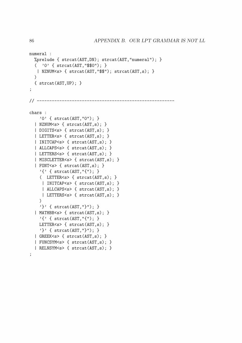
86 APPENDIX B. OUR LPT GRAMMAR IS NOT LL
numeral :
%prelude strcat(AST,DN); strcat(AST,"numeral");
( ’0’ strcat(AST,"$$0");
| NZNUM<s> strcat(AST,"$$"); strcat(AST,s);
)
strcat(AST,UP);
;
// -------------------------------------------------------
chars :
’0’ strcat(AST,"0");
| NZNUM<s> strcat(AST,s);
| DIGITS<s> strcat(AST,s);
| LETTER<s> strcat(AST,s);
| INITCAP<s> strcat(AST,s);
| ALLCAPS<s> strcat(AST,s);
| LETTERS<s> strcat(AST,s);
| MISCLETTER<s> strcat(AST,s);
| FONT<s> strcat(AST,s);
’’ strcat(AST,"");
( LETTER<s> strcat(AST,s);
| INITCAP<s> strcat(AST,s);
| ALLCAPS<s> strcat(AST,s);
| LETTERS<s> strcat(AST,s);
)
’’ strcat(AST,"");
| MATHBB<s> strcat(AST,s);
’’ strcat(AST,"");
LETTER<s> strcat(AST,s);
’’ strcat(AST,"");
| GREEK<s> strcat(AST,s);
| FUNCSYM<s> strcat(AST,s);
| RELNSYM<s> strcat(AST,s);
;

Appendix C
DAG depth and size data
In the tables below, find all the DAG depth and size measurements for the definitionsappearing in Appendices F and G.
C.1 Foundations – Suppes
Suppes Chapter 2Definiendum Depth Size∆0:infix 2 3×:infix 2 2
Suppes Chapter 3Definiendum Depth Size Definiendum Depth SizeBR:1 2 2 TR:1 2 2Dom:1 3 3 Rng:1 3 3Fld:1 4 6 Cnv:1 3 3:infix 3 3 |:infix 4 6|Rng:infix 5 7 RFX:2 3 3IRFX:2 3 3 SYM:2 3 3ASYM:2 3 3 ANSYM:2 3 3TRAN:2 3 3 CONN:2 3 3SCONN:2 3 3 RFX:1 5 8IRFX:1 5 8 SYM:1 4 5
87

88 APPENDIX C. DAG DEPTH AND SIZE DATA
Suppes Chapter 3, continuedDefiniendum Depth Size Definiendum Depth SizeASYM:1 4 5 ANSYM:1 4 5TRAN:1 4 5 CONN:1 4 5SCONN:1 4 5 Id:1 2 2QORD:2 4 5 PORD:2 4 6SORD:2 4 6 SPORD:2 4 5SSORD:2 4 6 QORD:1 5 10PORD:1 5 11 SORD:1 5 11SPORD:1 5 10 SSORD:1 5 11MELT:3 3 3 FELT:3 3 3WO:2 4 7 ISUC:3 3 3LELT:3 3 3 SECT:3 6 10Seg:3 3 3 LB:3 3 3INF:3 4 4 UB:3 3 3SUP:3 4 4 EQUIV:1 6 13EQUIV:2 7 14 Coset:2 7 14PART:2 2 4 PART:1 3 5FINER:2 4 7 Part:1 8 15Reln:1 4 7 FCN:1 2 2MONO:1 4 5 FCN:3 4 7SURJ:3 4 6 MONO:3 5 9BIJ:3 5 8 Maps:2 5 8
Suppes Chapter 4Definiendum Depth Size Definiendum Depth Size≈C:infix 6 9 ≤C:infix 7 11<C:infix 8 12 MNEL:2 1 1MXEL:2 1 1 FIN:1 3 5DFIN:1 7 11

C.1. FOUNDATIONS – SUPPES 89
Suppes Chapter 5Definiendum Depth Size Definiendum Depth SizeTRANS:1 1 1 ECONN:1 1 1ORD:1 2 3 Eps:1 2 2<O:infix 3 4 ≤O:infix 3 4>O:infix 3 4 ≥O:infix 3 4Suc:1 4 5 NAT:1 5 13ω:0 6 14 N:0 7 150N:0 2 2 1N:0 2 22N:0 5 8 3N:0 6 94N:0 7 10 5N:0 8 116N:0 9 12 7N:0 10 138N:0 11 14 9N:0 12 1510N:0 13 16 Addnat:0 7 18+N:infix 8 19 Mulnat:0 9 21·N:infix 10 22 Expnat:0 11 23ExpN:infix 12 24 INF:1 4 6DEN:1 7 21 DINF:1 8 12CNTBL:1 7 20 UNCNTBL:1 8 21
Suppes Chapter 6Definiendum Depth Size Definiendum Depth Size/:infix 7 16 Fr:0 8 17≡Fr:infix 11 24 <Fr:infix 11 25>Fr:infix 12 26 ≤Fr:infix 12 27≥Fr:infix 13 28 +Fr:infix 11 24·Fr:infix 11 24 Nra:0 12 38InclFrNra:1 12 38 <Nra:infix 13 41>Nra:infix 13 42 ≤Nra:infix 13 42≥Nra:infix 14 43 +Nra:infix 13 40·Nra:infix 13 40 0Nra:0 12 371Nra:0 12 37 ≡SUB:infix 14 41<SUB:infix 14 44 +SUB:infix 14 41·SUB:infix 14 43 Ra:0 15 43InclNraRa:1 15 43 InclFrRa:1 16 45

90 APPENDIX C. DAG DEPTH AND SIZE DATA
Suppes Chapter 6, continuedDefiniendum Depth Size Definiendum Depth Size
Q:0 16 44 <Ra:infix 16 48+Ra:infix 16 45 ·Ra:infix 16 470Ra:0 15 43 1Ra:0 15 44>Ra:infix 17 49 ≤Ra:infix 17 49≥Ra:infix 18 50 −Ra:infix 17 46AvRa:1 19 56 NatRa:0 18 57NRa:0 19 58 IntRa:0 19 58ZRa:0 20 59 SeqRa:0 16 47+SeqRa:infix 17 50 ·SeqRa:infix 17 52<N:infix 7 16 >N:infix 7 16≤N:infix 8 17 ≥N:infix 8 17CseqRa:0 20 63 ≡CseqRa:infix 20 59<CseqRa:infix 21 64 R:0 21 65<R:infix 22 67 >R:infix 23 68≤R:infix 23 68 ≥R:infix 24 69+R:infix 22 67 −R:infix 23 68·R:infix 22 71 0R:0 22 661R:0 22 68 AvR:1 25 74IdR:1 22 66 InclNraR:1 23 68InclFrR:1 23 70 RaR:0 23 67SeqR:0 22 66 CseqR:0 26 76Lim:1 26 76 UBR:2 24 69MinR:1 23 68 MaxR:1 23 68LubR:1 25 71 FinitesumsetR:1 23 71FinitesumR:1 24 72 SqrtR:1 25 77SupR:1 23 70 InfR:1 23 70
C.2 Topology – Munkres
Munkres Chapter 12Definiendum Depth Size Definiendum Depth SizeTOPOLOGY:2 3 6 TOPSP:2 4 7OPENSET:3 5 8 FINERTOP:3 5 9STRFINERTOP:3 5 9 COARSERTOP:3 5 8STRCOARSERTOP:3 5 8
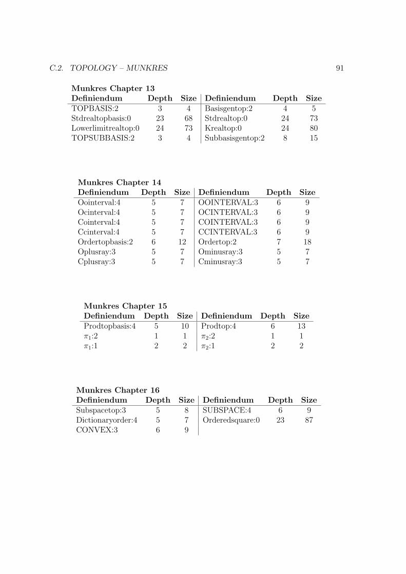
C.2. TOPOLOGY – MUNKRES 91
Munkres Chapter 13Definiendum Depth Size Definiendum Depth SizeTOPBASIS:2 3 4 Basisgentop:2 4 5Stdrealtopbasis:0 23 68 Stdrealtop:0 24 73Lowerlimitrealtop:0 24 73 Krealtop:0 24 80TOPSUBBASIS:2 3 4 Subbasisgentop:2 8 15
Munkres Chapter 14Definiendum Depth Size Definiendum Depth SizeOointerval:4 5 7 OOINTERVAL:3 6 9Ocinterval:4 5 7 OCINTERVAL:3 6 9Cointerval:4 5 7 COINTERVAL:3 6 9Ccinterval:4 5 7 CCINTERVAL:3 6 9Ordertopbasis:2 6 12 Ordertop:2 7 18Oplusray:3 5 7 Ominusray:3 5 7Cplusray:3 5 7 Cminusray:3 5 7
Munkres Chapter 15Definiendum Depth Size Definiendum Depth SizeProdtopbasis:4 5 10 Prodtop:4 6 13π1:2 1 1 π2:2 1 1π1:1 2 2 π2:1 2 2
Munkres Chapter 16Definiendum Depth Size Definiendum Depth SizeSubspacetop:3 5 8 SUBSPACE:4 6 9Dictionaryorder:4 5 7 Orderedsquare:0 23 87CONVEX:3 6 9

92 APPENDIX C. DAG DEPTH AND SIZE DATA
Munkres Chapter 17Definiendum Depth Size Definiendum Depth SizeCLOSEDSET:3 6 10 Interior:1 5 8Closure:3 7 12 INTERSECTS:2 2 3DISJOINT:2 2 3 NBHD:4 5 8LIMITPT:4 6 11 TOPCONV:3 8 29HAUSDORFF:2 5 9 TOPLIMIT:3 9 32
Munkres Chapter 18Definiendum Depth Size Definiendum Depth SizeCONTINUOUS:5 6 19 CONTAT:6 6 19HOMEOMORPHISM:5 7 22 HOMEOMORPHIC:4 8 23TOPIMBED:5 8 25
Munkres Chapter 19Definiendum Depth Size Definiendum Depth SizeTUPLE:3 4 5 Cartesprod:2 5 6Cartespow:2 6 7 Boxtopbasis:3 6 14Boxtop:3 7 17 Projection:3 6 7Prodtopsubbasis:3 7 20 Productspace:3 9 27
Munkres Chapter 20Definiendum Depth Size Definiendum Depth SizeMETRIC:2 25 73 Ball:4 26 74Metrictopbasis:2 27 75 Metrictop:2 28 80METRIZABLE:2 29 84 METRICSPACE:3 29 84BOUNDED:3 30 86 Diam:1 31 89Stdbddmetric:2 30 89 Rnnorm:2 26 87Rneuclideanmetric:3 27 89 Rnsqmetric:3 26 79Uniformmetric:3 31 110

C.2. TOPOLOGY – MUNKRES 93
Munkres Chapter 21Definiendum Depth Size Definiendum Depth SizeCNTBLBASISAT:3 8 26 FIRSTCNTBL:2 9 27UNIFCONV:7 30 86
Munkres Chapter 22Definiendum Depth Size Definiendum Depth SizeQUOTIENTMAP:5 6 18 SATURATED:5 6 19OPENMAP:5 6 17 CLOSEDMAP:5 7 20Quotienttop:3 7 19 QUOTIENTSPACE:2 8 21
Munkres Chapter 23Definiendum Depth SizeSEPARATION:4 5 10CONNECTED:2 6 11TOTALLYDISCONNECTED:2 7 23
Munkres Chapter 24Definiendum Depth Size Definiendum Depth SizeLINEARCONTINUUM:2 9 21 PATH:5 25 84PATHCONNECTED:2 26 85 Rnunitball:1 27 93Puncturedeuclideanspace:1 25 84 Unitsphere:1 27 92
Munkres Chapter 25Definiendum Depth Size Definiendum Depth SizeCcequiv:2 7 28 ∼CC :infix 8 29Components:2 9 40 Pcequiv:2 26 89∼PC :infix 27 90 Pathcomponents:2 27 91LOCALCONNAT:3 7 14 LOCALCONN:2 8 15LOCALPATHCONNAT:3 27 87 LOCALPATHCONN:2 28 88WEAKLOCALCONNAT:3 7 14
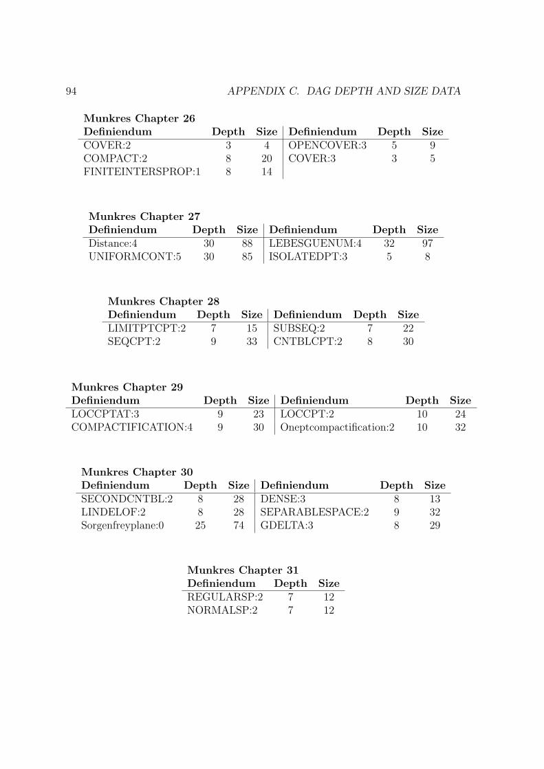
94 APPENDIX C. DAG DEPTH AND SIZE DATA
Munkres Chapter 26Definiendum Depth Size Definiendum Depth SizeCOVER:2 3 4 OPENCOVER:3 5 9COMPACT:2 8 20 COVER:3 3 5FINITEINTERSPROP:1 8 14
Munkres Chapter 27Definiendum Depth Size Definiendum Depth SizeDistance:4 30 88 LEBESGUENUM:4 32 97UNIFORMCONT:5 30 85 ISOLATEDPT:3 5 8
Munkres Chapter 28Definiendum Depth Size Definiendum Depth SizeLIMITPTCPT:2 7 15 SUBSEQ:2 7 22SEQCPT:2 9 33 CNTBLCPT:2 8 30
Munkres Chapter 29Definiendum Depth Size Definiendum Depth SizeLOCCPTAT:3 9 23 LOCCPT:2 10 24COMPACTIFICATION:4 9 30 Oneptcompactification:2 10 32
Munkres Chapter 30Definiendum Depth Size Definiendum Depth SizeSECONDCNTBL:2 8 28 DENSE:3 8 13LINDELOF:2 8 28 SEPARABLESPACE:2 9 32Sorgenfreyplane:0 25 74 GDELTA:3 8 29
Munkres Chapter 31Definiendum Depth SizeREGULARSP:2 7 12NORMALSP:2 7 12
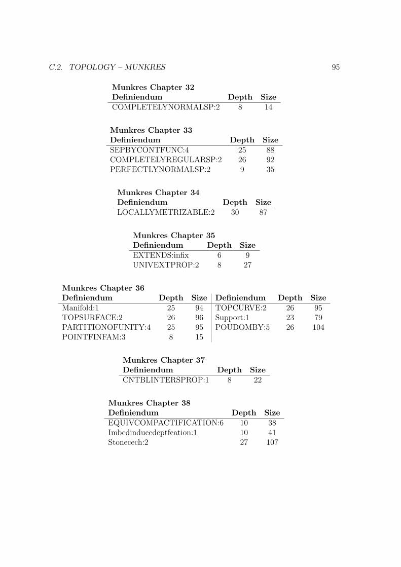
C.2. TOPOLOGY – MUNKRES 95
Munkres Chapter 32Definiendum Depth SizeCOMPLETELYNORMALSP:2 8 14
Munkres Chapter 33Definiendum Depth SizeSEPBYCONTFUNC:4 25 88COMPLETELYREGULARSP:2 26 92PERFECTLYNORMALSP:2 9 35
Munkres Chapter 34Definiendum Depth SizeLOCALLYMETRIZABLE:2 30 87
Munkres Chapter 35Definiendum Depth SizeEXTENDS:infix 6 9UNIVEXTPROP:2 8 27
Munkres Chapter 36Definiendum Depth Size Definiendum Depth SizeManifold:1 25 94 TOPCURVE:2 26 95TOPSURFACE:2 26 96 Support:1 23 79PARTITIONOFUNITY:4 25 95 POUDOMBY:5 26 104POINTFINFAM:3 8 15
Munkres Chapter 37Definiendum Depth SizeCNTBLINTERSPROP:1 8 22
Munkres Chapter 38Definiendum Depth SizeEQUIVCOMPACTIFICATION:6 10 38Imbedinducedcptfcation:1 10 41Stonecech:2 27 107

96 APPENDIX C. DAG DEPTH AND SIZE DATA

Appendix D
Quantifier depth data
We gathered eight data points for each definition in the database. In the followingtables, we use alpha for a definition’s translation into DZFC, E (α,∅) for the totalexpansion thereof, and E (α, B0) for the partial expansion, as explained in Section 4.2.
D.1 Foundations – Suppes
Suppes Chapter 2Nesting Alternating Nesting
Definiendum LPT α E (α,∅) E (α, B0) LPT α E (α,∅) E (α, B0)∆0:infix 0 0 4 0 0 0 4 0×:infix 0 2 4 2 0 2 3 2
Suppes Chapter 3Nesting Alternating Nesting
Definiendum LPT α E (α,∅) E (α, B0) LPT α E (α,∅) E (α, B0)BR:1 2 2 4 2 2 2 3 2TR:1 2 2 6 2 2 2 3 2Dom:1 1 3 5 3 1 2 3 2Rng:1 1 3 5 3 1 2 3 2Fld:1 0 0 7 3 0 0 5 2
97
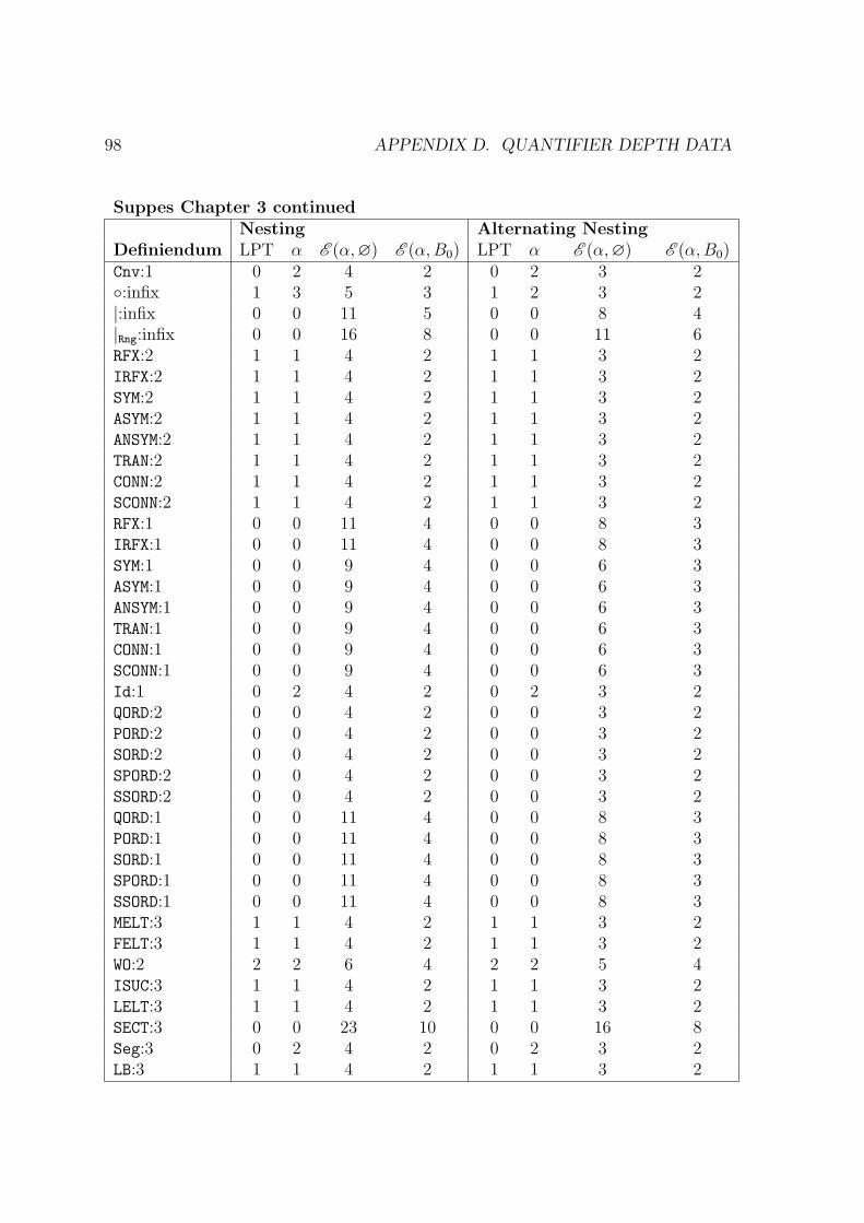
98 APPENDIX D. QUANTIFIER DEPTH DATA
Suppes Chapter 3 continuedNesting Alternating Nesting
Definiendum LPT α E (α,∅) E (α, B0) LPT α E (α,∅) E (α, B0)Cnv:1 0 2 4 2 0 2 3 2:infix 1 3 5 3 1 2 3 2|:infix 0 0 11 5 0 0 8 4|Rng:infix 0 0 16 8 0 0 11 6RFX:2 1 1 4 2 1 1 3 2IRFX:2 1 1 4 2 1 1 3 2SYM:2 1 1 4 2 1 1 3 2ASYM:2 1 1 4 2 1 1 3 2ANSYM:2 1 1 4 2 1 1 3 2TRAN:2 1 1 4 2 1 1 3 2CONN:2 1 1 4 2 1 1 3 2SCONN:2 1 1 4 2 1 1 3 2RFX:1 0 0 11 4 0 0 8 3IRFX:1 0 0 11 4 0 0 8 3SYM:1 0 0 9 4 0 0 6 3ASYM:1 0 0 9 4 0 0 6 3ANSYM:1 0 0 9 4 0 0 6 3TRAN:1 0 0 9 4 0 0 6 3CONN:1 0 0 9 4 0 0 6 3SCONN:1 0 0 9 4 0 0 6 3Id:1 0 2 4 2 0 2 3 2QORD:2 0 0 4 2 0 0 3 2PORD:2 0 0 4 2 0 0 3 2SORD:2 0 0 4 2 0 0 3 2SPORD:2 0 0 4 2 0 0 3 2SSORD:2 0 0 4 2 0 0 3 2QORD:1 0 0 11 4 0 0 8 3PORD:1 0 0 11 4 0 0 8 3SORD:1 0 0 11 4 0 0 8 3SPORD:1 0 0 11 4 0 0 8 3SSORD:1 0 0 11 4 0 0 8 3MELT:3 1 1 4 2 1 1 3 2FELT:3 1 1 4 2 1 1 3 2WO:2 2 2 6 4 2 2 5 4ISUC:3 1 1 4 2 1 1 3 2LELT:3 1 1 4 2 1 1 3 2SECT:3 0 0 23 10 0 0 16 8Seg:3 0 2 4 2 0 2 3 2LB:3 1 1 4 2 1 1 3 2

D.1. FOUNDATIONS – SUPPES 99
Suppes Chapter 3 continuedNesting Alternating Nesting
Definiendum LPT α E (α,∅) E (α, B0) LPT α E (α,∅) E (α, B0)INF:3 1 1 5 3 1 1 3 2UB:3 1 1 4 2 1 1 3 2SUP:3 1 1 5 3 1 1 3 2EQUIV:1 0 0 11 4 0 0 8 3EQUIV:2 0 0 11 4 0 0 8 3Coset:2 0 2 11 4 0 2 8 3PART:2 1 1 3 1 1 1 3 1PART:1 1 1 4 2 1 1 4 2FINER:2 2 2 4 2 2 2 4 2Part:1 0 2 13 6 0 2 10 5Reln:1 1 3 4 3 1 2 4 2FCN:1 0 2 4 2 0 2 3 2MONO:1 0 0 8 4 0 0 6 4FCN:3 0 0 6 3 0 0 3 2SURJ:3 0 0 5 3 0 0 3 2MONO:3 0 0 8 4 0 0 6 4BIJ:3 0 0 8 4 0 0 6 4Maps:2 0 2 8 5 0 2 5 4
Suppes Chapter 4Nesting Alternating Nesting
Definiendum LPT α E (α,∅) E (α, B0) LPT α E (α,∅) E (α, B0)≈C:infix 1 1 9 5 1 1 7 5≤C:infix 1 1 10 6 1 1 7 5<C:infix 0 0 10 6 0 0 7 5MNEL:2 1 1 1 1 1 1 1 1MXEL:2 1 1 1 1 1 1 1 1FIN:1 2 2 5 3 2 2 4 3DFIN:1 1 1 10 6 1 1 8 6

100 APPENDIX D. QUANTIFIER DEPTH DATA
Suppes Chapter 5Nesting Alternating Nesting
Definiendum LPT α E (α,∅) E (α, B0) LPT α E (α,∅) E (α, B0)TRANS:1 2 2 2 2 1 1 1 1ECONN:1 1 1 1 1 1 1 1 1ORD:1 0 0 2 2 0 0 1 1Eps:1 0 2 4 2 0 2 3 2<O:infix 0 0 2 2 0 0 1 1≤O:infix 0 0 2 2 0 0 1 1>O:infix 0 0 2 2 0 0 1 1≥O:infix 0 0 2 2 0 0 1 1Suc:1 0 2 4 4 0 2 3 3NAT:1 0 0 14 7 0 0 11 7ω:0 0 2 16 9 0 2 13 9
N:0 0 0 16 9 0 0 13 90N:0 0 0 2 0 0 0 2 01N:0 0 1 3 1 0 1 3 12N:0 0 0 7 5 0 0 6 43N:0 0 0 11 9 0 0 9 74N:0 0 0 15 13 0 0 12 105N:0 0 0 19 17 0 0 15 136N:0 0 0 23 21 0 0 18 167N:0 0 0 27 25 0 0 21 198N:0 0 0 31 29 0 0 24 229N:0 0 0 35 33 0 0 27 2510N:0 0 0 39 37 0 0 30 28Addnat:0 1 2 18 11 1 2 14 10+N:infix 0 1 19 12 0 1 14 10Mulnat:0 1 2 25 14 1 2 17 12·N:infix 0 1 26 15 0 1 17 12Expnat:0 1 2 28 17 1 2 19 14ExpN:infix 0 1 29 18 0 1 19 14INF:1 0 0 5 3 0 0 4 3DEN:1 0 0 25 14 0 0 20 14DINF:1 0 0 10 6 0 0 8 6CNTBL:1 1 1 25 14 1 1 20 14UNCNTBL:1 0 0 25 14 0 0 20 14
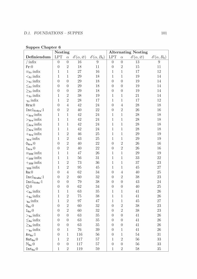
D.1. FOUNDATIONS – SUPPES 101
Suppes Chapter 6Nesting Alternating Nesting
Definiendum LPT α E (α,∅) E (α, B0) LPT α E (α,∅) E (α, B0)/:infix 0 0 16 9 0 0 13 9Fr:0 0 2 18 11 0 2 15 11≡Fr:infix 1 1 27 16 1 1 17 12<Fr:infix 1 1 29 18 1 1 19 14>Fr:infix 0 0 29 18 0 0 19 14≤Fr:infix 0 0 29 18 0 0 19 14≥Fr:infix 0 0 29 18 0 0 19 14+Fr:infix 1 2 38 19 1 1 21 14·Fr:infix 1 2 28 17 1 1 17 12Nra:0 0 4 42 24 0 4 28 18InclFrNra:1 0 2 40 22 0 2 26 16<Nra:infix 1 1 42 24 1 1 28 18>Nra:infix 1 1 42 24 1 1 28 18≤Nra:infix 1 1 42 24 1 1 28 18≥Nra:infix 1 1 42 24 1 1 28 18+Nra:infix 1 2 46 25 1 1 29 19·Nra:infix 1 2 43 25 1 1 29 190Nra:0 0 2 40 22 0 2 26 161Nra:0 0 2 40 22 0 2 26 16≡SUB:infix 1 1 47 26 1 1 29 19<SUB:infix 1 1 56 31 1 1 33 22+SUB:infix 1 2 73 36 1 1 37 23·SUB:infix 1 2 95 45 1 1 45 27Ra:0 0 4 62 34 0 4 40 25InclNraRa:1 0 2 60 32 0 2 38 23InclFrRa:1 0 0 79 38 0 0 43 24Q:0 0 0 62 34 0 0 40 25<Ra:infix 1 1 63 35 1 1 41 26+Ra:infix 1 2 75 38 1 1 41 26·Ra:infix 1 2 97 47 1 1 45 270Ra:0 0 2 60 32 0 2 38 231Ra:0 0 2 60 32 0 2 38 23>Ra:infix 0 0 63 35 0 0 41 26≤Ra:infix 0 0 63 35 0 0 41 26≥Ra:infix 0 0 63 35 0 0 41 26−Ra:infix 0 1 76 39 0 1 41 26AvRa:1 0 1 116 56 0 1 54 31NatRa:0 1 2 117 57 1 2 56 33NRa:0 0 0 117 57 0 0 56 33IntRa:0 1 2 119 59 1 2 58 35

102 APPENDIX D. QUANTIFIER DEPTH DATA
Suppes Chapter 6 continuedNesting Alternating Nesting
Definiendum LPT α E (α,∅) E (α, B0) LPT α E (α,∅) E (α, B0)ZRa:0 0 0 119 59 0 0 58 35SeqRa:0 0 0 70 39 0 0 45 29+SeqRa:infix 1 2 77 40 1 2 46 30·SeqRa:infix 1 2 99 49 1 2 47 30<N:infix 0 0 16 9 0 0 13 9>N:infix 0 0 16 9 0 0 13 9≤N:infix 0 0 16 9 0 0 13 9≥N:infix 0 0 16 9 0 0 13 9CseqRa:0 3 5 173 84 3 5 74 46≡CseqRa:infix 3 3 171 82 3 3 72 44<CseqRa:infix 3 3 173 84 2 2 74 46
R:0 0 4 186 90 0 4 84 51<R:infix 1 1 187 91 1 1 85 52>R:infix 0 0 187 91 0 0 85 52≤R:infix 0 0 187 91 0 0 85 52≥R:infix 0 0 187 91 0 0 85 52+R:infix 1 2 231 108 1 1 95 57−R:infix 0 1 232 109 0 1 95 57·R:infix 1 2 253 117 1 1 96 570R:0 2 3 187 91 2 2 85 521R:0 2 3 187 91 2 2 85 52AvR:1 0 1 401 185 0 1 153 89IdR:1 2 3 187 91 2 2 85 52InclNraR:1 0 0 187 91 0 0 85 52InclFrR:1 0 0 187 91 0 0 85 52RaR:0 0 2 189 93 0 2 86 53SeqR:0 0 0 194 95 0 0 89 55CseqR:0 3 5 547 250 3 5 199 116Lim:1 3 4 546 249 3 4 198 115UBR:2 1 1 188 92 1 1 86 53MinR:1 1 2 189 93 1 2 87 54MaxR:1 1 2 189 93 1 2 87 54LubR:1 0 2 288 138 0 2 121 74FinitesumsetR:1 2 2 233 110 2 2 97 59FinitesumR:1 1 1 234 111 1 1 97 59SqrtR:1 0 1 284 134 0 1 116 69SupR:1 0 3 195 96 0 3 90 55InfR:1 0 3 195 96 0 3 90 55

D.2. TOPOLOGY – MUNKRES 103
D.2 Topology – Munkres
Munkres Chapter 12Nesting Alternating Nesting
Definiendum LPT α E (α,∅) E (α, B0) LPT α E (α,∅) E (α, B0)TOPOLOGY:2 1 1 4 1 1 1 3 1TOPSP:2 0 0 4 1 0 0 3 1OPENSET:3 0 0 4 1 0 0 3 1FINERTOP:3 0 0 4 1 0 0 3 1STRFINERTOP:3 0 0 4 1 0 0 3 1COARSERTOP:3 0 0 4 1 0 0 3 1STRCOARSERTOP:3 0 0 4 1 0 0 3 1
Munkres Chapter 13Nesting Alternating Nesting
Definiendum LPT α E (α,∅) E (α, B0) LPT α E (α,∅) E (α, B0)TOPBASIS:2 3 3 6 3 2 2 4 2Basisgentop:2 3 4 6 4 2 3 4 3Stdrealtopbasis:0 1 5 192 96 1 4 88 55Stdrealtop:0 0 0 198 100 0 0 92 58Lowerlimitrealtop:0 1 5 198 100 1 4 92 58Krealtop:0 1 5 203 103 1 4 96 60TOPSUBBASIS:2 0 0 4 0 0 0 3 0Subbasisgentop:2 2 5 14 10 2 4 10 8

104 APPENDIX D. QUANTIFIER DEPTH DATA
Munkres Chapter 14Nesting Alternating Nesting
Definiendum LPT α E (α,∅) E (α, B0) LPT α E (α,∅) E (α, B0)Oointerval:4 0 2 4 2 0 2 3 2OOINTERVAL:3 1 1 5 3 1 1 4 3Ocinterval:4 0 2 4 2 0 2 3 2OCINTERVAL:3 1 1 5 3 1 1 4 3Cointerval:4 0 2 4 2 0 2 3 2COINTERVAL:3 1 1 5 3 1 1 4 3Ccinterval:4 0 2 4 2 0 2 3 2CCINTERVAL:3 1 1 5 3 1 1 4 3Ordertopbasis:2 1 3 7 5 1 2 5 4Ordertop:2 0 0 13 9 0 0 9 7Oplusray:3 0 2 4 2 0 2 3 2Ominusray:3 0 2 4 2 0 2 3 2Cplusray:3 0 2 4 2 0 2 3 2Cminusray:3 0 2 4 2 0 2 3 2
Munkres Chapter 15Nesting Alternating Nesting
Definiendum LPT α E (α,∅) E (α, B0) LPT α E (α,∅) E (α, B0)Prodtopbasis:4 0 2 6 4 0 2 5 4Prodtop:4 0 0 12 8 0 0 9 7π1:2 0 0 0 0 0 0 0 0π2:2 0 0 0 0 0 0 0 0π1:1 1 1 3 1 1 1 2 1π2:1 1 1 3 1 1 1 2 1
Munkres Chapter 16Nesting Alternating Nesting
Definiendum LPT α E (α,∅) E (α, B0) LPT α E (α,∅) E (α, B0)Subspacetop:3 0 2 4 2 0 2 4 2SUBSPACE:4 0 0 4 2 0 0 4 2Dictionaryorder:4 2 3 7 3 2 3 4 3Orderedsquare:0 0 2 196 96 0 2 90 56CONVEX:3 1 1 6 3 1 1 4 2

D.2. TOPOLOGY – MUNKRES 105
Munkres Chapter 17Nesting Alternating Nesting
Definiendum LPT α E (α,∅) E (α, B0) LPT α E (α,∅) E (α, B0)CLOSEDSET:3 0 0 6 1 0 0 5 1Interior:1 0 2 6 2 0 2 5 2Closure:3 0 2 11 3 0 2 9 3INTERSECTS:2 0 0 2 0 0 0 2 0DISJOINT:2 0 0 2 0 0 0 2 0NBHD:4 0 0 4 1 0 0 3 1LIMITPT:4 1 2 6 2 1 1 5 2TOPCONV:3 3 3 24 14 3 3 18 13HAUSDORFF:2 2 2 4 2 2 2 4 2TOPLIMIT:3 1 2 26 16 1 1 19 14
Munkres Chapter 18Nesting Alternating Nesting
Definiendum LPT α E (α,∅) E (α, B0) LPT α E (α,∅) E (α, B0)CONTINUOUS:5 1 1 21 11 1 1 14 8CONTAT:6 2 2 19 10 2 2 13 8HOMEOMORPHISM:5 0 0 25 13 0 0 17 10HOMEOMORPHIC:4 1 1 26 14 1 1 18 11TOPIMBED:5 0 0 34 17 0 0 24 13
Munkres Chapter 19Nesting Alternating Nesting
Definiendum LPT α E (α,∅) E (α, B0) LPT α E (α,∅) E (α, B0)TUPLE:3 1 1 5 3 1 1 3 2Cartesprod:2 0 2 7 5 0 2 5 4Cartespow:2 0 2 11 7 0 2 8 6Boxtopbasis:3 1 3 9 7 1 3 7 6Boxtop:3 1 1 17 11 1 1 12 9Projection:3 0 2 9 7 0 2 7 6Prodtopsubbasis:3 1 2 31 19 1 2 23 16Productspace:3 1 1 47 29 1 1 33 24

106 APPENDIX D. QUANTIFIER DEPTH DATA
Munkres Chapter 20Nesting Alternating Nesting
Definiendum LPT α E (α,∅) E (α, B0) LPT α E (α,∅) E (α, B0)METRIC:2 1 1 328 151 1 1 127 75Ball:4 0 2 328 151 0 2 127 75Metrictopbasis:2 0 2 330 153 0 2 129 77Metrictop:2 0 0 336 157 0 0 133 80METRIZABLE:2 1 1 337 158 1 1 134 80METRICSPACE:3 0 0 336 157 0 0 133 80BOUNDED:3 2 2 336 157 2 2 133 80Diam:1 0 3 336 157 0 3 133 80Stdbddmetric:2 1 3 336 157 1 2 133 80Rnnorm:2 0 2 704 318 0 2 242 139Rneuclideanmetric:3 0 0 912 409 0 0 314 178Rnsqmetric:3 0 2 546 249 0 2 197 114Uniformmetric:3 0 2 1235 552 0 2 422 239
Munkres Chapter 21Nesting Alternating Nesting
Definiendum LPT α E (α,∅) E (α, B0) LPT α E (α,∅) E (α, B0)CNTBLBASISAT:3 3 3 23 13 3 3 17 12FIRSTCNTBL:2 1 1 24 14 1 1 18 13UNIFCONV:7 4 4 336 157 3 3 133 80
Munkres Chapter 22Nesting Alternating Nesting
Definiendum LPT α E (α,∅) E (α, B0) LPT α E (α,∅) E (α, B0)QUOTIENTMAP:5 1 1 21 11 1 1 14 8SATURATED:5 1 2 23 11 1 1 16 9OPENMAP:5 1 1 17 9 1 1 11 6CLOSEDMAP:5 1 1 23 10 1 1 17 7Quotienttop:3 0 1 22 12 0 1 15 9QUOTIENTSPACE:2 1 2 22 12 1 2 15 9
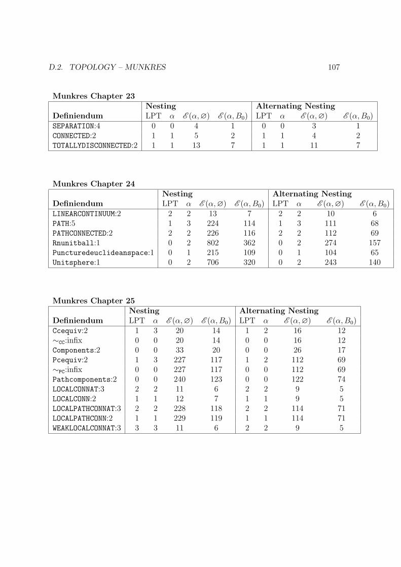
D.2. TOPOLOGY – MUNKRES 107
Munkres Chapter 23Nesting Alternating Nesting
Definiendum LPT α E (α,∅) E (α, B0) LPT α E (α,∅) E (α, B0)SEPARATION:4 0 0 4 1 0 0 3 1CONNECTED:2 1 1 5 2 1 1 4 2TOTALLYDISCONNECTED:2 1 1 13 7 1 1 11 7
Munkres Chapter 24Nesting Alternating Nesting
Definiendum LPT α E (α,∅) E (α, B0) LPT α E (α,∅) E (α,B0)LINEARCONTINUUM:2 2 2 13 7 2 2 10 6PATH:5 1 3 224 114 1 3 111 68PATHCONNECTED:2 2 2 226 116 2 2 112 69Rnunitball:1 0 2 802 362 0 2 274 157Puncturedeuclideanspace:1 0 1 215 109 0 1 104 65Unitsphere:1 0 2 706 320 0 2 243 140
Munkres Chapter 25Nesting Alternating Nesting
Definiendum LPT α E (α,∅) E (α, B0) LPT α E (α,∅) E (α, B0)Ccequiv:2 1 3 20 14 1 2 16 12∼CC:infix 0 0 20 14 0 0 16 12Components:2 0 0 33 20 0 0 26 17Pcequiv:2 1 3 227 117 1 2 112 69∼PC:infix 0 0 227 117 0 0 112 69Pathcomponents:2 0 0 240 123 0 0 122 74LOCALCONNAT:3 2 2 11 6 2 2 9 5LOCALCONN:2 1 1 12 7 1 1 9 5LOCALPATHCONNAT:3 2 2 228 118 2 2 114 71LOCALPATHCONN:2 1 1 229 119 1 1 114 71WEAKLOCALCONNAT:3 3 3 11 6 2 2 9 5
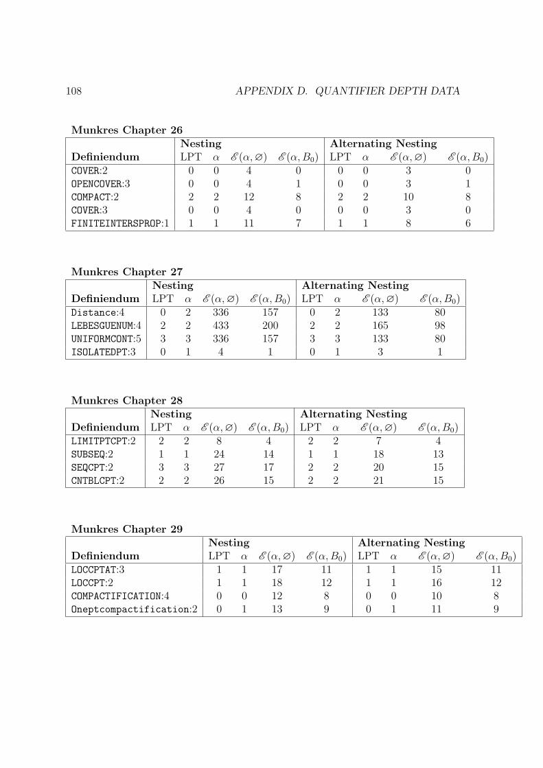
108 APPENDIX D. QUANTIFIER DEPTH DATA
Munkres Chapter 26Nesting Alternating Nesting
Definiendum LPT α E (α,∅) E (α, B0) LPT α E (α,∅) E (α, B0)COVER:2 0 0 4 0 0 0 3 0OPENCOVER:3 0 0 4 1 0 0 3 1COMPACT:2 2 2 12 8 2 2 10 8COVER:3 0 0 4 0 0 0 3 0FINITEINTERSPROP:1 1 1 11 7 1 1 8 6
Munkres Chapter 27Nesting Alternating Nesting
Definiendum LPT α E (α,∅) E (α, B0) LPT α E (α,∅) E (α, B0)Distance:4 0 2 336 157 0 2 133 80LEBESGUENUM:4 2 2 433 200 2 2 165 98UNIFORMCONT:5 3 3 336 157 3 3 133 80ISOLATEDPT:3 0 1 4 1 0 1 3 1
Munkres Chapter 28Nesting Alternating Nesting
Definiendum LPT α E (α,∅) E (α, B0) LPT α E (α,∅) E (α, B0)LIMITPTCPT:2 2 2 8 4 2 2 7 4SUBSEQ:2 1 1 24 14 1 1 18 13SEQCPT:2 3 3 27 17 2 2 20 15CNTBLCPT:2 2 2 26 15 2 2 21 15
Munkres Chapter 29Nesting Alternating Nesting
Definiendum LPT α E (α,∅) E (α, B0) LPT α E (α,∅) E (α, B0)LOCCPTAT:3 1 1 17 11 1 1 15 11LOCCPT:2 1 1 18 12 1 1 16 12COMPACTIFICATION:4 0 0 12 8 0 0 10 8Oneptcompactification:2 0 1 13 9 0 1 11 9

D.2. TOPOLOGY – MUNKRES 109
Munkres Chapter 30Nesting Alternating Nesting
Definiendum LPT α E (α,∅) E (α, B0) LPT α E (α,∅) E (α, B0)SECONDCNTBL:2 1 1 26 15 1 1 20 14DENSE:3 0 0 11 3 0 0 9 3LINDELOF:2 2 2 27 16 2 2 21 15SEPARABLESPACE:2 1 1 26 15 1 1 20 14Sorgenfreyplane:0 0 0 204 102 0 0 95 59GDELTA:3 1 3 26 15 1 3 20 14
Munkres Chapter 31Nesting Alternating Nesting
Definiendum LPT α E (α,∅) E (α, B0) LPT α E (α,∅) E (α, B0)REGULARSP:2 3 3 8 3 2 2 7 2NORMALSP:2 2 2 8 3 2 2 7 2
Munkres Chapter 32Nesting Alternating Nesting
Definiendum LPT α E (α,∅) E (α, B0) LPT α E (α,∅) E (α, B0)COMPLETELYNORMALSP:2 1 1 12 5 1 1 10 4
Munkres Chapter 33Nesting Alternating Nesting
Definiendum LPT α E (α,∅) E (α, B0) LPT α E (α,∅) E (α, B0)SEPBYCONTFUNC:4 1 3 224 114 1 3 111 68COMPLETELYREGULARSP:2 2 3 226 116 1 1 112 69PERFECTLYNORMALSP:2 1 1 27 16 1 1 21 15
Munkres Chapter 34Nesting Alternating Nesting
Definiendum LPT α E (α,∅) E (α, B0) LPT α E (α,∅) E (α, B0)LOCALLYMETRIZABLE:2 2 2 339 160 2 2 135 81

110 APPENDIX D. QUANTIFIER DEPTH DATA
Munkres Chapter 35Nesting Alternating Nesting
Definiendum LPT α E (α,∅) E (α, B0) LPT α E (α,∅) E (α, B0)EXTENDS:infix 1 1 8 5 1 1 5 4UNIVEXTPROP:2 2 2 26 14 2 2 18 10
Munkres Chapter 36Nesting Alternating Nesting
Definiendum LPT α E (α,∅) E (α, B0) LPT α E (α,∅) E (α, B0)Manifold:1 3 5 244 128 2 4 125 79TOPCURVE:2 0 0 244 128 0 0 125 79TOPSURFACE:2 0 0 244 128 0 0 125 79Support:1 0 1 217 103 0 1 108 62PARTITIONOFUNITY:4 1 3 235 112 1 2 98 60POUDOMBY:5 1 2 235 112 1 2 109 62POINTFINFAM:3 1 3 15 9 1 2 11 8
Munkres Chapter 37Nesting Alternating Nesting
Definiendum LPT α E (α,∅) E (α, B0) LPT α E (α,∅) E (α, B0)CNTBLINTERSPROP:1 1 1 26 15 1 1 21 15
Munkres Chapter 38Nesting Alternating Nesting
Definiendum LPT α E (α,∅) E (α, B0) LPT α E (α,∅) E (α, B0)EQUIVCOMPACTIFICATION:6 2 2 26 14 2 2 18 11Imbedinducedcptfcation:1 1 3 37 20 1 2 26 15Stonecech:2 2 5 226 116 2 5 112 69

Appendix E
Symbol count data
We display three counts for each definition α: (1) In the column headed 0 we givethe number of symbols in the definiens of α; (2) in the column headed A we give thenumber of symbols in E (α,∅), i.e., the full expansion of α; (3) in the column headedB we give the number of symbols in E (α, B0), where B0 is the set of foundationaldefinitions given in Section 4.2.
In these tables, we put a ceiling on the symbol count of any expanded definition: at231−1 symbols (the maximum value for an integer in the Java programming language),we say “enough is enough”. In the tables, this is recorded as ‘2147483647+’. We couldhave easily gone to higher numbers, but the point is already made: the raw symbolcount for expanded definitions goes exponentially, and rapidly gets out of hand.
E.1 Foundations – Suppes
Suppes Chapter 2Definiendum 0 A B∆0:infix 31 300 31×:infix 112 270 112
111

112 APPENDIX E. SYMBOL COUNT DATA
Suppes Chapter 3Definiendum 0 A BBR:1 66 224 66TR:1 83 571 83Dom:1 141 518 202Rng:1 141 518 202Fld:1 19 1128 411Cnv:1 146 681 207:infix 199 1111 321|:infix 61 1138 419|Rng:infix 46 3046 1134RFX:2 67 444 128IRFX:2 73 450 134SYM:2 123 658 184ASYM:2 125 660 186ANSYM:2 132 667 193TRAN:2 166 859 227CONN:2 136 671 197SCONN:2 112 647 173RFX:1 26 1803 612IRFX:1 27 1809 618SYM:1 26 1924 660ASYM:1 27 1926 662ANSYM:1 28 1933 669TRAN:1 27 2642 904CONN:1 27 1937 673SCONN:1 28 1913 649Id:1 95 253 95QORD:2 25 1311 363PORD:2 43 1986 564

E.1. FOUNDATIONS – SUPPES 113
Suppes Chapter 3, continuedDefiniendum 0 A BSORD:2 45 2189 609SPORD:2 26 1527 421SSORD:2 43 2206 626QORD:1 14 5819 2003PORD:1 14 8748 3024SORD:1 14 10078 3479SPORD:1 15 7162 2471SSORD:1 15 10095 3496MELT:3 88 465 149FELT:3 106 483 167WO:2 113 1303 439ISUC:3 119 812 180LELT:3 106 483 167SECT:3 73 9576 3105Seg:3 147 524 208LB:3 67 444 128INF:3 93 1121 331UB:3 67 444 128SUP:3 93 1121 331EQUIV:1 35 6385 2192EQUIV:2 26 7525 2615Coset:2 153 7810 2742PART:2 179 468 179PART:1 20 479 190FINER:2 126 1094 492Part:1 133 15432 5454Reln:1 175 805 358FCN:1 130 446 130MONO:1 25 2260 680FCN:3 51 1539 567SURJ:3 42 1506 558MONO:3 52 3353 1117BIJ:3 43 3320 1108Maps:2 84 1613 641

114 APPENDIX E. SYMBOL COUNT DATA
Suppes Chapter 4Definiendum 0 A B≈C:infix 21 3331 1119≤C:infix 51 3390 1154<C:infix 40 6794 2322MNEL:2 61 61 61MXEL:2 61 61 61FIN:1 116 348 168DFIN:1 86 3425 1189
Suppes Chapter 5Definiendum 0 A BTRANS:1 73 73 73ECONN:1 82 82 82ORD:1 24 163 163Eps:1 127 285 127<O:infix 35 349 349≤O:infix 46 360 360>O:infix 35 349 349≥O:infix 46 360 360Suc:1 123 627 627NAT:1 31 7714 2900ω:0 80 7788 2974
N:0 6 7788 29740N:0 11 61 111N:0 61 111 612N:0 10 1727 12273N:0 10 17887 128874N:0 10 179487 1294875N:0 10 1795487 12954876N:0 10 17955487 129554877N:0 10 179555487 1295554878N:0 10 1795555487 12955554879N:0 10 2147483647+ 2147483647+10N:0 10 2147483647+ 2147483647+

E.1. FOUNDATIONS – SUPPES 115
Suppes Chapter 5, continuedDefiniendum 0 A BAddnat:0 402 40263 13927+N:infix 77 40822 13998Mulnat:0 418 158150 40334·N:infix 77 158709 40405Expnat:0 422 276087 66791ExpN:infix 77 276646 66862INF:1 12 354 174DEN:1 21 11118 4092DINF:1 13 3431 1195CNTBL:1 26 11118 4092UNCNTBL:1 14 11124 4098
Suppes Chapter 6Definiendum 0 A B/:infix 100 15878 6042Fr:0 107 31851 12179≡Fr:infix 87 349221 92941<Fr:infix 92 1619229 416517>Fr:infix 11 1619229 416517≤Fr:infix 33 1968456 509464≥Fr:infix 33 1968456 509464+Fr:infix 183 3067779 153452·Fr:infix 161 365167 99051Nra:0 196 10873248 2898930InclFrNra:1 153 10873205 2898887<Nra:infix 89 23365797 6214449>Nra:infix 89 23365797 6214449≤Nra:infix 92 23715024 6307396≥Nra:infix 92 23715024 6307396+Nra:infix 176 36036884 8943323·Nra:infix 180 33334272 88889220Nra:0 128 10890479 28991541Nra:0 128 10890929 2899354≡SUB:infix 101 72074161 17886723
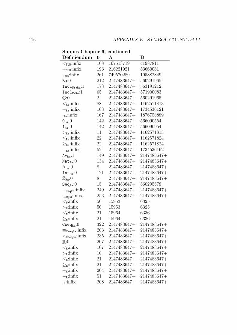
116 APPENDIX E. SYMBOL COUNT DATA
Suppes Chapter 6, continuedDefiniendum 0 A B<SUB:infix 108 167513719 41987811+SUB:infix 193 216221921 53660081·SUB:infix 261 749570289 195882849Ra:0 212 2147483647+ 560291965InclNraRa:1 173 2147483647+ 563191212InclFrRa:1 65 2147483647+ 571900083Q:0 2 2147483647+ 560291965<Ra:infix 88 2147483647+ 1162571813+Ra:infix 163 2147483647+ 1734536121·Ra:infix 167 2147483647+ 18767588890Ra:0 142 2147483647+ 5660905541Ra:0 142 2147483647+ 566090954>Ra:infix 11 2147483647+ 1162571813≤Ra:infix 22 2147483647+ 1162571824≥Ra:infix 22 2147483647+ 1162571824−Ra:infix 52 2147483647+ 1734536162AvRa:1 149 2147483647+ 2147483647+NatRa:0 134 2147483647+ 2147483647+NRa:0 8 2147483647+ 2147483647+IntRa:0 121 2147483647+ 2147483647+ZRa:0 8 2147483647+ 2147483647+SeqRa:0 15 2147483647+ 560295578+SeqRa:infix 249 2147483647+ 2147483647+·SeqRa:infix 253 2147483647+ 2147483647+<N:infix 50 15953 6325>N:infix 50 15953 6325≤N:infix 21 15964 6336≥N:infix 21 15964 6336CseqRa:0 322 2147483647+ 2147483647+≡CseqRa:infix 203 2147483647+ 2147483647+<CseqRa:infix 235 2147483647+ 2147483647+
R:0 207 2147483647+ 2147483647+<R:infix 107 2147483647+ 2147483647+>R:infix 10 2147483647+ 2147483647+≤R:infix 21 2147483647+ 2147483647+≥R:infix 21 2147483647+ 2147483647++R:infix 204 2147483647+ 2147483647+−R:infix 51 2147483647+ 2147483647+·R:infix 208 2147483647+ 2147483647+

E.2. TOPOLOGY – MUNKRES 117
Suppes Chapter 6, continuedDefiniendum 0 A B0R:0 170 2147483647+ 2147483647+1R:0 170 2147483647+ 2147483647+AvR:1 151 2147483647+ 2147483647+IdR:1 165 2147483647+ 2147483647+InclNraR:1 60 2147483647+ 2147483647+InclFrR:1 58 2147483647+ 2147483647+RaR:0 90 2147483647+ 2147483647+SeqR:0 23 2147483647+ 2147483647+CseqR:0 318 2147483647+ 2147483647+Lim:1 271 2147483647+ 2147483647+UBR:2 101 2147483647+ 2147483647+MinR:1 154 2147483647+ 2147483647+MaxR:1 154 2147483647+ 2147483647+LubR:1 145 2147483647+ 2147483647+FinitesumsetR:1 526 2147483647+ 2147483647+FinitesumR:1 187 2147483647+ 2147483647+SqrtR:1 150 2147483647+ 2147483647+SupR:1 146 2147483647+ 2147483647+InfR:1 146 2147483647+ 2147483647+
E.2 Topology – Munkres
Munkres Chapter 12Definiendum 0 A BTOPOLOGY:2 194 587 194TOPSP:2 13 587 194OPENSET:3 25 602 209FINERTOP:3 52 1230 420STRFINERTOP:3 71 1249 439COARSERTOP:3 52 1230 420STRCOARSERTOP:3 71 1249 439

118 APPENDIX E. SYMBOL COUNT DATA
Munkres Chapter 13Definiendum 0 A BTOPBASIS:2 252 493 252Basisgentop:2 261 919 500Stdrealtopbasis:0 303 2147483647+ 2147483647+Stdrealtop:0 39 2147483647+ 2147483647+Lowerlimitrealtop:0 330 2147483647+ 2147483647+Krealtop:0 319 2147483647+ 2147483647+TOPSUBBASIS:2 38 270 38Subbasisgentop:2 320 4101 1502
Munkres Chapter 14Definiendum 0 A BOointerval:4 209 2721 825OOINTERVAL:3 111 5033 1533Ocinterval:4 220 2732 836OCINTERVAL:3 111 5044 1544Cointerval:4 220 2732 836COINTERVAL:3 111 5044 1544Ccinterval:4 231 2743 847CCINTERVAL:3 111 5055 1555Ordertopbasis:2 277 11545 3645Ordertop:2 71 72417 23018Oplusray:3 165 2519 781Ominusray:3 165 2519 781Cplusray:3 176 2530 792Cminusray:3 176 2530 792
Munkres Chapter 15Definiendum 0 A BProdtopbasis:4 164 1577 633Prodtop:4 92 11585 4716π1:2 1 1 1π2:2 1 1 1π1:1 64 222 64π2:1 64 222 64

E.2. TOPOLOGY – MUNKRES 119
Munkres Chapter 16Definiendum 0 A BSubspacetop:3 151 839 335SUBSPACE:4 64 1486 565Dictionaryorder:4 324 5678 1556Orderedsquare:0 448 2147483647+ 2147483647+CONVEX:3 125 5071 1547
Munkres Chapter 17Definiendum 0 A BCLOSEDSET:3 65 1346 444Interior:1 171 898 355Closure:3 178 2240 790INTERSECTS:2 29 166 29DISJOINT:2 23 160 23NBHD:4 57 634 241LIMITPT:4 168 1633 594TOPCONV:3 237 34696 13524HAUSDORFF:2 184 908 378TOPLIMIT:3 112 70356 27482
Munkres Chapter 18Definiendum 0 A BCONTINUOUS:5 117 12024 4088CONTAT:6 201 7606 2810HOMEOMORPHISM:5 111 41496 13620HOMEOMORPHIC:4 73 42699 14037TOPIMBED:5 137 97964 34966
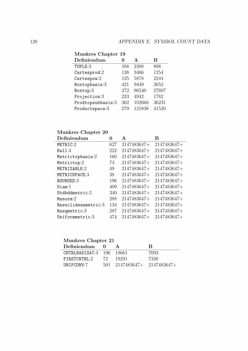
120 APPENDIX E. SYMBOL COUNT DATA
Munkres Chapter 19Definiendum 0 A BTUPLE:3 168 2388 808Cartesprod:2 138 3466 1254Cartespow:2 125 5878 2244Boxtopbasis:3 421 9449 3052Boxtop:3 272 86540 27607Projection:3 223 4942 1782Prodtopsubbasis:3 362 102666 36231Productspace:3 279 121838 41520
Munkres Chapter 20Definiendum 0 A BMETRIC:2 627 2147483647+ 2147483647+Ball:4 222 2147483647+ 2147483647+Metrictopbasis:2 160 2147483647+ 2147483647+Metrictop:2 73 2147483647+ 2147483647+METRIZABLE:2 49 2147483647+ 2147483647+METRICSPACE:3 38 2147483647+ 2147483647+BOUNDED:3 196 2147483647+ 2147483647+Diam:1 409 2147483647+ 2147483647+Stdbddmetric:2 340 2147483647+ 2147483647+Rnnorm:2 288 2147483647+ 2147483647+Rneuclideanmetric:3 134 2147483647+ 2147483647+Rnsqmetric:3 287 2147483647+ 2147483647+Uniformmetric:3 474 2147483647+ 2147483647+
Munkres Chapter 21Definiendum 0 A BCNTBLBASISAT:3 196 18661 7093FIRSTCNTBL:2 72 19291 7330UNIFCONV:7 501 2147483647+ 2147483647+

E.2. TOPOLOGY – MUNKRES 121
Munkres Chapter 22Definiendum 0 A BQUOTIENTMAP:5 144 11966 4030SATURATED:5 286 21532 7257OPENMAP:5 107 5824 2154CLOSEDMAP:5 125 11547 4161Quotienttop:3 137 14727 5057QUOTIENTSPACE:2 227 17608 6150
Munkres Chapter 23Definiendum 0 A BSEPARATION:4 142 1051 336CONNECTED:2 59 1668 560TOTALLYDISCONNECTED:2 124 20867 8008
Munkres Chapter 24Definiendum 0 A BLINEARCONTINUUM:2 370 11660 3854PATH:5 510 2147483647+ 2147483647+PATHCONNECTED:2 97 2147483647+ 2147483647+Rnunitball:1 184 2147483647+ 2147483647+Puncturedeuclideanspace:1 290 2147483647+ 2147483647+Unitsphere:1 198 2147483647+ 2147483647+
Munkres Chapter 25Definiendum 0 A BCcequiv:2 292 48386 25947∼CC:infix 82 49191 26201Components:2 56 1274057 680272Pcequiv:2 202 2147483647+ 2147483647+∼PC:infix 82 2147483647+ 2147483647+Pathcomponents:2 56 2147483647+ 2147483647+LOCALCONNAT:3 161 18725 7342LOCALCONN:2 71 19355 7579LOCALPATHCONNAT:3 165 2147483647+ 2147483647+LOCALPATHCONN:2 75 2147483647+ 2147483647+WEAKLOCALCONNAT:3 196 18784 7377
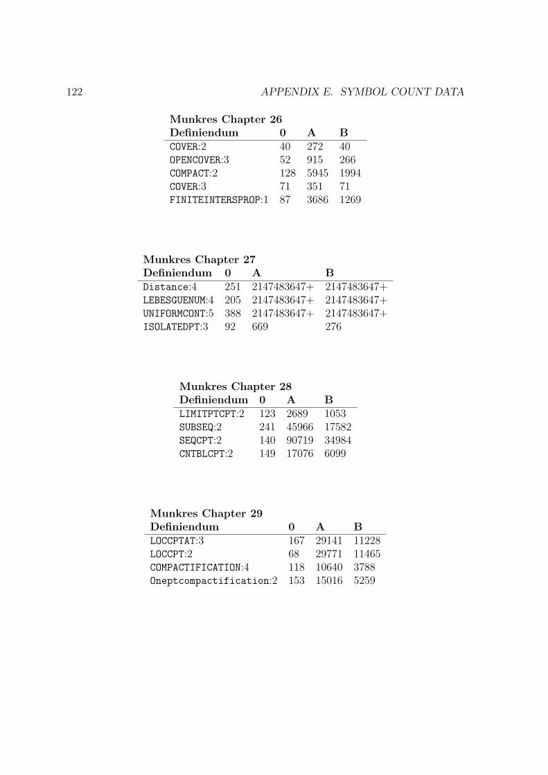
122 APPENDIX E. SYMBOL COUNT DATA
Munkres Chapter 26Definiendum 0 A BCOVER:2 40 272 40OPENCOVER:3 52 915 266COMPACT:2 128 5945 1994COVER:3 71 351 71FINITEINTERSPROP:1 87 3686 1269
Munkres Chapter 27Definiendum 0 A BDistance:4 251 2147483647+ 2147483647+LEBESGUENUM:4 205 2147483647+ 2147483647+UNIFORMCONT:5 388 2147483647+ 2147483647+ISOLATEDPT:3 92 669 276
Munkres Chapter 28Definiendum 0 A BLIMITPTCPT:2 123 2689 1053SUBSEQ:2 241 45966 17582SEQCPT:2 140 90719 34984CNTBLCPT:2 149 17076 6099
Munkres Chapter 29Definiendum 0 A BLOCCPTAT:3 167 29141 11228LOCCPT:2 68 29771 11465COMPACTIFICATION:4 118 10640 3788Oneptcompactification:2 153 15016 5259
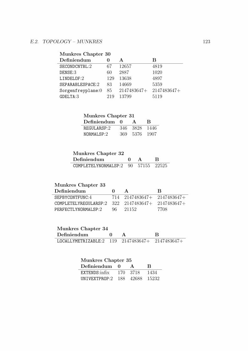
E.2. TOPOLOGY – MUNKRES 123
Munkres Chapter 30Definiendum 0 A BSECONDCNTBL:2 67 12657 4819DENSE:3 60 2887 1020LINDELOF:2 129 13638 4897SEPARABLESPACE:2 83 14669 5359Sorgenfreyplane:0 85 2147483647+ 2147483647+GDELTA:3 219 13799 5119
Munkres Chapter 31Definiendum 0 A BREGULARSP:2 346 3828 1446NORMALSP:2 369 5376 1907
Munkres Chapter 32Definiendum 0 A BCOMPLETELYNORMALSP:2 90 57155 22525
Munkres Chapter 33Definiendum 0 A BSEPBYCONTFUNC:4 714 2147483647+ 2147483647+COMPLETELYREGULARSP:2 322 2147483647+ 2147483647+PERFECTLYNORMALSP:2 96 21152 7708
Munkres Chapter 34Definiendum 0 A BLOCALLYMETRIZABLE:2 119 2147483647+ 2147483647+
Munkres Chapter 35Definiendum 0 A BEXTENDS:infix 170 3718 1434UNIVEXTPROP:2 188 42688 15232

124 APPENDIX E. SYMBOL COUNT DATA
Munkres Chapter 36Definiendum 0 A BManifold:1 396 2147483647+ 2147483647+TOPCURVE:2 35 2147483647+ 2147483647+TOPSURFACE:2 35 2147483647+ 2147483647+Support:1 174 2147483647+ 2147483647+PARTITIONOFUNITY:4 592 2147483647+ 2147483647+POUDOMBY:5 313 2147483647+ 2147483647+POINTFINFAM:3 198 6056 2268
Munkres Chapter 37Definiendum 0 A BCNTBLINTERSPROP:1 88 11379 4172
Munkres Chapter 38Definiendum 0 A BEQUIVCOMPACTIFICATION:6 182 63042 21304Imbedinducedcptfcation:1 222 210584 75294Stonecech:2 378 2147483647+ 2147483647+

Appendix F
Definitions: Foundations – Suppes
In his paper on the Proofless Text system [11], Friedman formalizes the definitionsfrom Chapters 2 through 6 of Suppes’s Axiomatic Set Theory, [15]. I have parsed andtranslated all of those definitions, with a few additional ones added in, as they wereneeded for the Munkres Topology definitions.
For each of these definitions, find below a triplet, consisting of:
i. A transcription of the definition into LPT input,
ii. The LATEX version of the input, and
iii. The DZFC translation of the definition, as performed by lpt2dzfc.
Side-by-side comparison of these definitions against the originals as they appearin [15] will reveal how good of an approximation to the original is possible in LPT.
F.1 Chapter 2
DEFINITION FS.1.1: Infix function \Delta_0. x \Delta_0 y \simeq
(x \less y) \cup (y \less x). Precedence 60.
DEFINITION FS.1.1: Infix function ∆0. x ∆0 y ' (x\y) ∪ (y\x). Precedence 60.
∆0(x, y) ' ∪((\(x, y)), (\(y, x)))
125

126 APPENDIX F. DEFINITIONS: FOUNDATIONS – SUPPES
DEFINITION FS.1.2: Infix function \times. x \times y \simeq
<z,w> : z \in x \wedge w \in y
. Precedence 20.
DEFINITION FS.1.2: Infix function ×. x× y ' 〈z, w〉 : z ∈x ∧ w∈ y. Precedence20.
×(x, y) ' (ιy0)(∀x0)(x0 ∈ y0 ↔ (∃z, w)(x0 = $0(z, w) ∧ (z ∈ x ∧ w ∈ y)))
F.2 Chapter 3
DEFINITION FS.2.1: 1-ary relation BR. BR[A] \iff (\forall y \in A)
(\exists z,w)(y = <z,w>).
DEFINITION FS.2.1: 1-ary relation BR. BR[A] ↔ (∀y ∈A)(∃z, w)(y = 〈z, w〉).BR[A] ↔ (∀y)(y ∈ A → (∃z, w)y = $0(z, w))
DEFINITION FS.2.2: 1-ary relation TR. TR[A] \iff (\forall y \in A)
(\exists z,w,u)(y = <z,w,u>).
DEFINITION FS.2.2: 1-ary relation TR. TR[A] ↔ (∀y ∈A)(∃z, w, u)(y = 〈z, w, u〉).TR[A] ↔ (∀y)(y ∈ A → (∃z, w, u)y = $0($0(z, w), u))
DEFINITION FS.2.3: 1-ary function Dom. If BR[R] then Dom(R) \simeq
x : (\exists y)(x \infixrlR y). Otherwise Dom(R) \up.
DEFINITION FS.2.3: 1-ary function Dom. If BR[R] then Dom(R) ' x : (∃y)(xRy).Otherwise Dom(R)↑.Dom(R) ' (ιz0)((BR[R] ∧ z0 ' (ιy0)(∀x0)(x0 ∈ y0 ↔ (∃x)(x0 = x ∧ ((∃y) $0(x, y) ∈R)))))

F.2. CHAPTER 3 127
DEFINITION FS.2.4: 1-ary function Rng. If BR[R] then Rng(R) \simeq
y : (\exists x)(x \infixrlR y). Otherwise Rng(R) \up.
DEFINITION FS.2.4: 1-ary function Rng. If BR[R] then Rng(R) ' y : (∃x)(xRy).Otherwise Rng(R)↑.Rng(R) ' (ιz0)((BR[R] ∧ z0 ' (ιy0)(∀x0)(x0 ∈ y0 ↔ (∃y)(x0 = y ∧ ((∃x) $0(x, y) ∈R)))))
DEFINITION FS.2.5: 1-ary function Fld. Fld(R) \simeq
Dom(R) \cup Rng(R).
DEFINITION FS.2.5: 1-ary function Fld. Fld(R) ' Dom(R) ∪ Rng(R).
Fld(R) ' ∪(Dom(R), Rng(R))
DEFINITION FS.2.6: 1-ary function Cnv. If BR[R] then Cnv(R) \simeq
<x,y> : y \infixrlR x. Otherwise Cnv(R) \up.
DEFINITION FS.2.6: 1-ary function Cnv. If BR[R] then Cnv(R) ' 〈x, y〉 : yRx.Otherwise Cnv(R)↑.Cnv(R) ' (ιz0)((BR[R]∧z0 ' (ιy0)(∀x0)(x0 ∈ y0 ↔ (∃x, y)(x0 = $0(x, y)∧($0(y, x) ∈R)))))
DEFINITION FS.2.8: Infix function \circ. If BR[R] \wedge BR[S] then
R \circ S \simeq <x,y> : (\exists z)(x \infixrlR z \wedge
z \infixrlS y). Otherwise R \circ S \up. Precedence 10.
DEFINITION FS.2.8: Infix function . If BR[R] ∧ BR[S] then R S ' 〈x, y〉 :(∃z)(xRz ∧ zSy). Otherwise R S↑. Precedence 10.
(R, S) ' (ιz0)((BR[R] ∧ BR[S] ∧ z0 ' (ιy0)(∀x0)(x0 ∈ y0 ↔ (∃x, y)(x0 = $0(x, y) ∧((∃z) $0(x, z) ∈ R ∧$0(z, y) ∈ S)))))

128 APPENDIX F. DEFINITIONS: FOUNDATIONS – SUPPES
DEFINITION FS.2.9: Infix function |. If BR[R] then R|A \simeq R \cap
(A \times Rng(R)). Otherwise R|A \up. Precedence 5.
DEFINITION FS.2.9: Infix function |. If BR[R] then R |A ' R ∩ (A × Rng(R)).Otherwise R |A↑. Precedence 5.
|(R,A) ' (ιx0)((BR[R] ∧ x0 ' ∩(R, (×(A, Rng(R))))))
DEFINITION FS.2.10: Infix function |_Rng. If BR[R] then R |_Rng
A \simeq Rng(R|A). Otherwise R |_Rng A \up. Precedence 5.
DEFINITION FS.2.10: Infix function |Rng. If BR[R] then R |Rng A ' Rng(R|A). Oth-erwise R |Rng A↑. Precedence 5.
|Rng(R,A) ' (ιx0)((BR[R] ∧ x0 ' Rng(|(R, A))))
DEFINITION FS.2.11: 2-ary relation RFX. RFX[R,A] \iff BR[R] \wedge
(\forall x \in A)(x \infixrlR x).
DEFINITION FS.2.11: 2-ary relation RFX. RFX[R, A] ↔ BR[R] ∧ (∀x∈A)(xRx).
RFX[R, A] ↔ BR[R] ∧ (∀x)(x ∈ A → $0(x, x) ∈ R)
DEFINITION FS.2.12: 2-ary relation IRFX. IRFX[R,A] \iff BR[R] \wedge
(\forall x \in A)(\neg(x \infixrlR x)).
DEFINITION FS.2.12: 2-ary relation IRFX. IRFX[R, A] ↔ BR[R]∧(∀x∈A)(¬(xRx)).
IRFX[R, A] ↔ BR[R] ∧ (∀x)(x ∈ A → ¬($0(x, x) ∈ R))
DEFINITION FS.2.13: 2-ary relation SYM. SYM[R,A] \iff BR[R] \wedge
(\forall x,y \in A)(x \infixrlR y \iff y \infixrlR x).

F.2. CHAPTER 3 129
DEFINITION FS.2.13: 2-ary relation SYM. SYM[R, A] ↔ BR[R] ∧ (∀x, y ∈A)(xRy ↔yRx).
SYM[R, A] ↔ BR[R] ∧ (∀x, y)(x ∈ A ∧ y ∈ A → $0(x, y) ∈ R ↔ $0(y, x) ∈ R)
DEFINITION FS.2.14: 2-ary relation ASYM. ASYM[R,A] \iff BR[R] \wedge
(\forall x,y \in A)(x \infixrlR y \implies \neg(y \infixrlR x)).
DEFINITION FS.2.14: 2-ary relation ASYM. ASYM[R,A] ↔ BR[R]∧(∀x, y ∈A)(xRy →¬(yRx)).
ASYM[R, A] ↔ BR[R] ∧ (∀x, y)(x ∈ A ∧ y ∈ A → $0(x, y) ∈ R → ¬($0(y, x) ∈ R))
DEFINITION FS.2.15: 2-ary relation ANSYM. ANSYM[R,A] \iff BR[R] \wedge
(\forall x,y \in A)(
x \infixrlR y \wedge y \infixrlR x \implies x = y
).
DEFINITION FS.2.15: 2-ary relation ANSYM. ANSYM[R,A] ↔ BR[R]∧(∀x, y ∈A)(xRy∧yRx → x = y).
ANSYM[R, A] ↔ BR[R]∧(∀x, y)(x ∈ A∧y ∈ A → $0(x, y) ∈ R∧$0(y, x) ∈ R → x = y)
DEFINITION FS.2.16: 2-ary relation TRAN. TRAN[R,A] \iff BR[R] \wedge
(\forall x,y,z \in A)(x \infixrlR y \wedge y \infixrlR z
\implies x \infixrlR z).
DEFINITION FS.2.16: 2-ary relation TRAN. TRAN[R,A] ↔ BR[R]∧(∀x, y, z ∈A)(xRy∧yRz → xRz).
TRAN[R, A] ↔ BR[R] ∧ (∀x, y, z)(x ∈ A ∧ y ∈ A ∧ z ∈ A → $0(x, y) ∈ R ∧$0(y, z) ∈R → $0(x, z) ∈ R)

130 APPENDIX F. DEFINITIONS: FOUNDATIONS – SUPPES
DEFINITION FS.2.17: 2-ary relation CONN. CONN[R,A] \iff BR[R] \wedge
(\forall x,y \in A)(
x \neq y \implies x \infixrlR y \vee y \infixrlR x
).
DEFINITION FS.2.17: 2-ary relation CONN. CONN[R,A] ↔ BR[R] ∧ (∀x, y ∈A)(x 6=y → xRy ∨ yRx).
CONN[R, A] ↔ BR[R]∧ (∀x, y)(x ∈ A∧y ∈ A → ¬(x = y) → $0(x, y) ∈ R∨$0(y, x) ∈R)
DEFINITION FS.2.18: 2-ary relation SCONN. SCONN[R,A] \iff BR[R]
\wedge (\forall x,y \in A)(x \infixrlR y \vee y \infixrlR x).
DEFINITION FS.2.18: 2-ary relation SCONN. SCONN[R,A] ↔ BR[R]∧(∀x, y ∈A)(xRy∨yRx).
SCONN[R, A] ↔ BR[R] ∧ (∀x, y)(x ∈ A ∧ y ∈ A → $0(x, y) ∈ R ∨$0(y, x) ∈ R)
DEFINITION FS.2.19: 1-ary relation RFX. RFX[R] \iff BR[R] \wedge
RFX[R,Fld(R)].
DEFINITION FS.2.19: 1-ary relation RFX. RFX[R] ↔ BR[R] ∧ RFX[R, Fld(R)].
RFX[R] ↔ BR[R] ∧ RFX[R, Fld(R)]
DEFINITION FS.2.20: 1-ary relation IRFX. IRFX[R] \iff BR[R] \wedge
IRFX[R,Fld(R)].
DEFINITION FS.2.20: 1-ary relation IRFX. IRFX[R] ↔ BR[R] ∧ IRFX[R, Fld(R)].
IRFX[R] ↔ BR[R] ∧ IRFX[R, Fld(R)]
F.2. CHAPTER 3 131
DEFINITION FS.2.21: 1-ary relation SYM. SYM[R] \iff BR[R] \wedge
SYM[R,Dom(R)].
DEFINITION FS.2.21: 1-ary relation SYM. SYM[R] ↔ BR[R] ∧ SYM[R, Dom(R)].
SYM[R] ↔ BR[R] ∧ SYM[R, Dom(R)]
DEFINITION FS.2.22: 1-ary relation ASYM. ASYM[R] \iff BR[R] \wedge
ASYM[R,Dom(R)].
DEFINITION FS.2.22: 1-ary relation ASYM. ASYM[R] ↔ BR[R] ∧ ASYM[R, Dom(R)].
ASYM[R] ↔ BR[R] ∧ ASYM[R, Dom(R)]
DEFINITION FS.2.23: 1-ary relation ANSYM. ANSYM[R] \iff BR[R] \wedge
ANSYM[R,Dom(R)].
DEFINITION FS.2.23: 1-ary relation ANSYM. ANSYM[R] ↔ BR[R] ∧ ANSYM[R, Dom(R)].
ANSYM[R] ↔ BR[R] ∧ ANSYM[R, Dom(R)]
DEFINITION FS.2.24: 1-ary relation TRAN. TRAN[R] \iff BR[R] \wedge
TRAN[R,Dom(R)].
DEFINITION FS.2.24: 1-ary relation TRAN. TRAN[R] ↔ BR[R] ∧ TRAN[R, Dom(R)].
TRAN[R] ↔ BR[R] ∧ TRAN[R, Dom(R)]
DEFINITION FS.2.25: 1-ary relation CONN. CONN[R] \iff BR[R] \wedge
CONN[R,Dom(R)].
132 APPENDIX F. DEFINITIONS: FOUNDATIONS – SUPPES
DEFINITION FS.2.25: 1-ary relation CONN. CONN[R] ↔ BR[R] ∧ CONN[R, Dom(R)].
CONN[R] ↔ BR[R] ∧ CONN[R, Dom(R)]
DEFINITION FS.2.26: 1-ary relation SCONN. SCONN[R] \iff BR[R] \wedge
SCONN[R,Dom(R)].
DEFINITION FS.2.26: 1-ary relation SCONN. SCONN[R] ↔ BR[R] ∧ SCONN[R, Dom(R)].
SCONN[R] ↔ BR[R] ∧ SCONN[R, Dom(R)]
DEFINITION FS.2.27: 1-ary function Id. Id(x) \simeq <y,y> : y \in x.
DEFINITION FS.2.27: 1-ary function Id. Id(x) ' 〈y, y〉 : y ∈x.
Id(x) ' (ιy0)(∀x0)(x0 ∈ y0 ↔ (∃y)(x0 = $0(y, y) ∧ (y ∈ x)))
DEFINITION FS.2.28: 2-ary relation QORD. QORD[R,A] \iff RFX[R,A] \wedge
TRAN[R,A].
DEFINITION FS.2.28: 2-ary relation QORD. QORD[R, A] ↔ RFX[R, A] ∧ TRAN[R, A].
QORD[R, A] ↔ RFX[R, A] ∧ TRAN[R,A]
DEFINITION FS.2.29: 2-ary relation PORD. PORD[R,A] \iff RFX[R,A]
\wedge ANSYM[R,A] \wedge TRAN[R,A].
DEFINITION FS.2.29: 2-ary relation PORD. PORD[R, A] ↔ RFX[R,A]∧ ANSYM[R,A]∧TRAN[R, A].
PORD[R, A] ↔ RFX[R, A] ∧ ANSYM[R, A] ∧ TRAN[R, A]

F.2. CHAPTER 3 133
DEFINITION FS.2.30: 2-ary relation SORD. SORD[R,A] \iff ANSYM[R,A]
\wedge TRAN[R,A] \wedge SCONN[R,A].
DEFINITION FS.2.30: 2-ary relation SORD. SORD[R, A] ↔ ANSYM[R, A]∧TRAN[R, A]∧SCONN[R, A].
SORD[R, A] ↔ ANSYM[R,A] ∧ TRAN[R, A] ∧ SCONN[R, A]
DEFINITION FS.2.31: 2-ary relation SPORD. SPORD[R,A] \iff ASYM[R,A]
\wedge TRAN[R,A].
DEFINITION FS.2.31: 2-ary relation SPORD. SPORD[R,A] ↔ ASYM[R, A]∧TRAN[R, A].
SPORD[R, A] ↔ ASYM[R,A] ∧ TRAN[R, A]
DEFINITION FS.2.32: 2-ary relation SSORD. SSORD[R,A] \iff ASYM[R,A]
\wedge TRAN[R,A] \wedge CONN[R,A].
DEFINITION FS.2.32: 2-ary relation SSORD. SSORD[R,A] ↔ ASYM[R, A]∧TRAN[R,A]∧CONN[R, A].
SSORD[R, A] ↔ ASYM[R,A] ∧ TRAN[R, A] ∧ CONN[R, A]
DEFINITION FS.2.33: 1-ary relation QORD. QORD[R] \iff QORD[R,Fld(R)].
DEFINITION FS.2.33: 1-ary relation QORD. QORD[R] ↔ QORD[R, Fld(R)].
QORD[R] ↔ QORD[R, Fld(R)]
DEFINITION FS.2.34: 1-ary relation PORD. PORD[R] \iff PORD[R,Fld(R)].
134 APPENDIX F. DEFINITIONS: FOUNDATIONS – SUPPES
DEFINITION FS.2.34: 1-ary relation PORD. PORD[R] ↔ PORD[R, Fld(R)].
PORD[R] ↔ PORD[R, Fld(R)]
DEFINITION FS.2.35: 1-ary relation SORD. SORD[R] \iff SORD[R,Fld(R)].
DEFINITION FS.2.35: 1-ary relation SORD. SORD[R] ↔ SORD[R, Fld(R)].
SORD[R] ↔ SORD[R, Fld(R)]
DEFINITION FS.2.36: 1-ary relation SPORD. SPORD[R] \iff
SPORD[R,Fld(R)].
DEFINITION FS.2.36: 1-ary relation SPORD. SPORD[R] ↔ SPORD[R, Fld(R)].
SPORD[R] ↔ SPORD[R, Fld(R)]
DEFINITION FS.2.37: 1-ary relation SSORD. SSORD[R] \iff
SSORD[R,Fld(R)].
DEFINITION FS.2.37: 1-ary relation SSORD. SSORD[R] ↔ SSORD[R, Fld(R)].
SSORD[R] ↔ SSORD[R, Fld(R)]
DEFINITION FS.2.38: 3-ary relation MELT. MELT[x,R,A] \iff BR[R]
\wedge x \in A \wedge (\forall y \in A)(\neg(y \infixrlR x)).
DEFINITION FS.2.38: 3-ary relation MELT. MELT[x,R,A] ↔ BR[R]∧x∈A∧ (∀y ∈A)(¬(yRx)).
MELT[x,R,A] ↔ BR[R] ∧ x ∈ A ∧ (∀y)(y ∈ A → ¬($0(y, x) ∈ R))

F.2. CHAPTER 3 135
DEFINITION FS.2.39: 3-ary relation FELT. FELT[x,R,A] \iff BR[R] \wedge
x \in A \wedge (\forall y \in A)(x \neq y \implies x \infixrlR y).
DEFINITION FS.2.39: 3-ary relation FELT. FELT[x,R,A] ↔ BR[R]∧x∈A∧ (∀y ∈A)(x 6= y → xRy).
FELT[x,R,A] ↔ BR[R] ∧ x ∈ A ∧ (∀y)(y ∈ A → ¬(x = y) → $0(x, y) ∈ R)
DEFINITION FS.2.40: 2-ary relation WO. WO[R,A] \iff CONN[R,A] \wedge
(\forall B \subseteq A)(
B \neq \varnothing \implies (\exists x)(MELT[x,R,B])
).
DEFINITION FS.2.40: 2-ary relation WO. WO[R, A] ↔ CONN[R,A] ∧ (∀B⊆A)(B 6=∅→ (∃x)(MELT[x,R,B])).
WO[R,A] ↔ CONN[R, A] ∧ (∀B)(⊆[B, A] → ¬(B = ∅) → (∃x) MELT[x,R,B])
DEFINITION FS.2.41: 3-ary relation ISUC. ISUC[y,R,x] \iff BR[R]
\wedge x \infixrlR y \wedge (\forall z)(
x \infixrlR z \implies z = y \vee y \infixrlR z
).
DEFINITION FS.2.41: 3-ary relation ISUC. ISUC[y, R, x] ↔ BR[R]∧xRy∧(∀z)(xRz →z = y ∨ yRz).
ISUC[y,R, x] ↔ BR[R] ∧$0(x, y) ∈ R ∧ (∀z) $0(x, z) ∈ R → z = y ∨$0(y, z) ∈ R
DEFINITION FS.2.42: 3-ary relation LELT. LELT[x,R,A] \iff BR[R] \wedge
x \in A \wedge (\forall y \in A)(x \neq y \implies y \infixrlR x).
DEFINITION FS.2.42: 3-ary relation LELT. LELT[x,R,A] ↔ BR[R]∧x∈A∧ (∀y ∈A)(x 6= y → yRx).
LELT[x,R,A] ↔ BR[R] ∧ x ∈ A ∧ (∀y)(y ∈ A → ¬(x = y) → $0(y, x) ∈ R)
136 APPENDIX F. DEFINITIONS: FOUNDATIONS – SUPPES
DEFINITION FS.2.43: 3-ary relation SECT. SECT[B,R,A] \iff BR[R] \wedge
B \subseteq A \wedge A \cap Cnv(R) |_Rng B \subseteq B.
DEFINITION FS.2.43: 3-ary relation SECT. SECT[B,R,A] ↔ BR[R] ∧ B⊆A ∧ A ∩Cnv(R)|RngB⊆B.
SECT[B, R, A] ↔ BR[R] ∧ ⊆[B,A] ∧ ⊆[∩(A, |Rng(Cnv(R), B)), B]
DEFINITION FS.2.44: 3-ary function Seg. If BR[R] then Seg(A,R,x)
\simeq y \in A : y \infixrlR x. Otherwise Seg(R) \up.
DEFINITION FS.2.44: 3-ary function Seg. If BR[R] then Seg(A,R, x) ' y ∈A :yRx. Otherwise Seg(R)↑.
Seg(A,R, x) ' (ιz0)((BR[R] ∧ z0 ' (ιy0)(∀x0)(x0 ∈ y0 ↔ (∃y)(x0 = y ∧ ($0(y, x) ∈R) ∧ (y ∈ A)))))
DEFINITION FS.2.45: 3-ary relation LB. LB[x,R,A] \iff BR[R] \wedge
(\forall y \in A)(x \infixrlR y).
DEFINITION FS.2.45: 3-ary relation LB. LB[x,R, A] ↔ BR[R] ∧ (∀y ∈A)(xRy).
LB[x,R, A] ↔ BR[R] ∧ (∀y)(y ∈ A → $0(x, y) ∈ R)
DEFINITION FS.2.46: 3-ary relation INF. INF[x,R,A] \iff LB[x,R,A]
\wedge (\forall y \in A)(LB[y,R,A] \implies y \infixrlR x).
DEFINITION FS.2.46: 3-ary relation INF. INF[x,R, A] ↔ LB[x,R, A] ∧ (∀y ∈A)(LB[y,R, A] → yRx).
INF[x,R,A] ↔ LB[x,R, A] ∧ (∀y)(y ∈ A → LB[y,R, A] → $0(y, x) ∈ R)
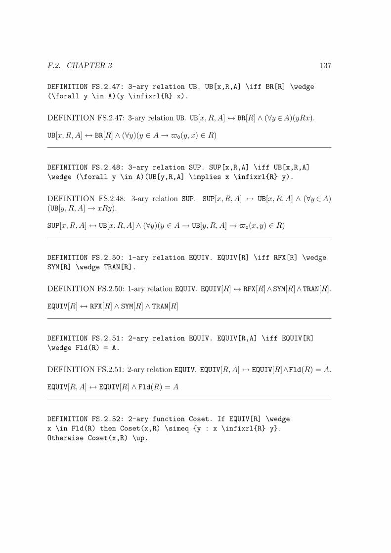
F.2. CHAPTER 3 137
DEFINITION FS.2.47: 3-ary relation UB. UB[x,R,A] \iff BR[R] \wedge
(\forall y \in A)(y \infixrlR x).
DEFINITION FS.2.47: 3-ary relation UB. UB[x,R, A] ↔ BR[R] ∧ (∀y ∈A)(yRx).
UB[x,R, A] ↔ BR[R] ∧ (∀y)(y ∈ A → $0(y, x) ∈ R)
DEFINITION FS.2.48: 3-ary relation SUP. SUP[x,R,A] \iff UB[x,R,A]
\wedge (\forall y \in A)(UB[y,R,A] \implies x \infixrlR y).
DEFINITION FS.2.48: 3-ary relation SUP. SUP[x,R, A] ↔ UB[x,R, A] ∧ (∀y ∈A)(UB[y,R, A] → xRy).
SUP[x,R,A] ↔ UB[x,R, A] ∧ (∀y)(y ∈ A → UB[y,R, A] → $0(x, y) ∈ R)
DEFINITION FS.2.50: 1-ary relation EQUIV. EQUIV[R] \iff RFX[R] \wedge
SYM[R] \wedge TRAN[R].
DEFINITION FS.2.50: 1-ary relation EQUIV. EQUIV[R] ↔ RFX[R]∧SYM[R]∧TRAN[R].
EQUIV[R] ↔ RFX[R] ∧ SYM[R] ∧ TRAN[R]
DEFINITION FS.2.51: 2-ary relation EQUIV. EQUIV[R,A] \iff EQUIV[R]
\wedge Fld(R) = A.
DEFINITION FS.2.51: 2-ary relation EQUIV. EQUIV[R,A] ↔ EQUIV[R]∧Fld(R) = A.
EQUIV[R, A] ↔ EQUIV[R] ∧ Fld(R) = A
DEFINITION FS.2.52: 2-ary function Coset. If EQUIV[R] \wedge
x \in Fld(R) then Coset(x,R) \simeq y : x \infixrlR y.
Otherwise Coset(x,R) \up.

138 APPENDIX F. DEFINITIONS: FOUNDATIONS – SUPPES
DEFINITION FS.2.52: 2-ary function Coset. If EQUIV[R]∧x∈ Fld(R) then Coset(x,R)' y : xRy. Otherwise Coset(x,R)↑.Coset(x,R) ' (ιz0)((EQUIV[R] ∧ x ∈ Fld(R) ∧ z0 ' (ιy0)(∀x0)(x0 ∈ y0 ↔ (∃y)(x0 =y ∧ ($0(x, y) ∈ R)))))
DEFINITION FS.2.53: 2-ary relation PART. PART[W,A] \iff
\cup(W) = A \wedge (\forall B,C \in W)(
B \neq C \implies B \cap C = \varnothing
) \wedge
(\forall B \in W)(B \neq \varnothing).
DEFINITION FS.2.53: 2-ary relation PART. PART[W,A] ↔ ∪(W ) = A∧ (∀B,C ∈W )(B 6= C → B ∩ C = ∅) ∧ (∀B ∈W )(B 6= ∅).
PART[W,A] ↔ ∪(W ) = A ∧ (∀B, C)(B ∈ W ∧ C ∈ W → ¬(B = C) → ∩(B, C) =∅) ∧ (∀B)(B ∈ W → ¬(B = ∅))
DEFINITION FS.2.54: 1-ary relation PART. PART[W] \iff
(\exists A)(PART[W,A]).
DEFINITION FS.2.54: 1-ary relation PART. PART[W ] ↔ (∃A)(PART[W,A]).
PART[W ] ↔ (∃A) PART[W,A]
DEFINITION FS.2.55: 2-ary relation FINER. If PART[V] \wedge PART[W]
then FINER[V,W] \iff V \neq W \wedge
(\forall A \in V)(\exists B \in W)(A \subseteq B).
DEFINITION FS.2.55: 2-ary relation FINER. If PART[V ]∧PART[W ] then FINER[V,W ] ↔V 6= W ∧ (∀A∈V )(∃B ∈W )(A⊆B).
FINER[V, W ] ↔ (PART[V ] ∧ PART[W ] ∧ ¬(V = W ) ∧ (∀A)(A ∈ V → (∃B)(B ∈W ∧ ⊆[A,B])))

F.2. CHAPTER 3 139
DEFINITION FS.2.56: 1-ary function Part. If EQUIV[R] then Part(R)
\simeq Coset(x,R) : x \in Fld(R).
DEFINITION FS.2.56: 1-ary function Part. If EQUIV[R] then Part(R) ' Coset(x,R) :x∈ Fld(R).Part(R) ' (ιz0)(EQUIV[R] ∧ z0 ' (ιy0)(∀x0)(x0 ∈ y0 ↔ (∃x,R)(x0 = Coset(x, R) ∧(x ∈ Fld(R)))))
DEFINITION FS.2.57: 1-ary function Reln. If PART[W] then Reln(W)
\simeq
<x,y> : (\exists B \in W)(x \in B \wedge y \in B)
.
DEFINITION FS.2.57: 1-ary function Reln. If PART[W ] then Reln(W ) ' 〈x, y〉 :(∃B ∈W )(x∈B ∧ y ∈B).Reln(W ) ' (ιz0)(PART[W ] ∧ z0 ' (ιy0)(∀x0)(x0 ∈ y0 ↔ (∃x, y)(x0 = $0(x, y) ∧((∃B)(B ∈ W ∧ x ∈ B ∧ y ∈ B)))))
DEFINITION FS.2.58: 1-ary relation FCN. FCN[f] \iff
f = <x,y> : f(x) = y.
DEFINITION FS.2.58: 1-ary relation FCN. FCN[f ] ↔ f = 〈x, y〉 : f(x) = y.FCN[f ] ↔ f = (ιz0)(∀y0)(y0 ∈ z0 ↔ (∃x, y)(y0 = $0(x, y) ∧ ((ιx0)($0(x, x0) ∈ f) =y)))
DEFINITION FS.2.59: 1-ary relation MONO. MONO[f] \iff FCN[f] \wedge
FCN[Cnv(f)].
DEFINITION FS.2.59: 1-ary relation MONO. MONO[f ] ↔ FCN[f ] ∧ FCN[Cnv(f)].
MONO[f ] ↔ FCN[f ] ∧ FCN[Cnv(f)]

140 APPENDIX F. DEFINITIONS: FOUNDATIONS – SUPPES
DEFINITION FS.2.60: 3-ary relation FCN. FCN[f,A,B] \iff FCN[f] \wedge
Dom(f) = A \wedge Rng(f) \subseteq B.
DEFINITION FS.2.60: 3-ary relation FCN. FCN[f, A,B] ↔ FCN[f ] ∧ Dom(f) = A ∧Rng(f)⊆B.
FCN[f, A,B] ↔ FCN[f ] ∧ Dom(f) = A ∧ ⊆[Rng(f), B]
DEFINITION FS.2.61: 3-ary relation SURJ. SURJ[f,A,B] \iff FCN[f]
\wedge Dom(f) = A \wedge Rng(f) = B.
DEFINITION FS.2.61: 3-ary relation SURJ. SURJ[f,A, B] ↔ FCN[f ] ∧ Dom(f) =A ∧ Rng(f) = B.
SURJ[f, A,B] ↔ FCN[f ] ∧ Dom(f) = A ∧ Rng(f) = B
DEFINITION FS.2.62: 3-ary relation MONO. MONO[f,A,B] \iff MONO[f]
\wedge Dom(f) = A \wedge Rng(f) \subseteq B.
DEFINITION FS.2.62: 3-ary relation MONO. MONO[f, A, B] ↔ MONO[f ] ∧ Dom(f) =A ∧ Rng(f)⊆B.
MONO[f, A,B] ↔ MONO[f ] ∧ Dom(f) = A ∧ ⊆[Rng(f), B]
DEFINITION FS.2.63: 3-ary relation BIJ. BIJ[f,A,B] \iff MONO[f]
\wedge Dom(f) = A \wedge Rng(f) = B.
DEFINITION FS.2.63: 3-ary relation BIJ. BIJ[f, A,B] ↔ MONO[f ] ∧ Dom(f) = A ∧Rng(f) = B.
BIJ[f, A,B] ↔ MONO[f ] ∧ Dom(f) = A ∧ Rng(f) = B
DEFINITION FS.2.64: 2-ary function Maps. Maps(A,B) \simeq
f : FCN[f,A,B].
DEFINITION FS.2.64: 2-ary function Maps. Maps(A,B) ' f : FCN[f, A,B].Maps(A,B) ' (ιy0)(∀x0)(x0 ∈ y0 ↔ (∃f)(x0 = f ∧ (FCN[f, A,B])))
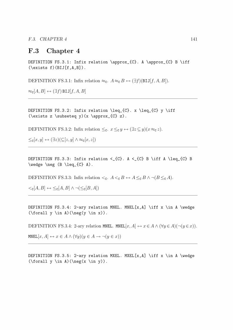
F.3. CHAPTER 4 141
F.3 Chapter 4
DEFINITION FS.3.1: Infix relation \approx_C. A \approx_C B \iff
(\exists f)(BIJ[f,A,B]).
DEFINITION FS.3.1: Infix relation ≈C. A≈C B ↔ (∃f)(BIJ[f,A, B]).
≈C[A,B] ↔ (∃f) BIJ[f,A, B]
DEFINITION FS.3.2: Infix relation \leq_C. x \leq_C y \iff
(\exists z \subseteq y)(x \approx_C z).
DEFINITION FS.3.2: Infix relation ≤C. x≤C y ↔ (∃z⊆ y)(x≈C z).
≤C[x, y] ↔ (∃z)(⊆[z, y] ∧ ≈C[x, z])
DEFINITION FS.3.3: Infix relation <_C. A <_C B \iff A \leq_C B
\wedge \neg (B \leq_C A).
DEFINITION FS.3.3: Infix relation <C. A<C B ↔ A≤C B ∧ ¬(B≤C A).
<C[A,B] ↔ ≤C[A,B] ∧ ¬(≤C[B, A])
DEFINITION FS.3.4: 2-ary relation MNEL. MNEL[x,A] \iff x \in A \wedge
(\forall y \in A)(\neg(y \in x)).
DEFINITION FS.3.4: 2-ary relation MNEL. MNEL[x,A] ↔ x∈A ∧ (∀y ∈A)(¬(y ∈x)).
MNEL[x,A] ↔ x ∈ A ∧ (∀y)(y ∈ A → ¬(y ∈ x))
DEFINITION FS.3.5: 2-ary relation MXEL. MXEL[x,A] \iff x \in A \wedge
(\forall y \in A)(\neg(x \in y)).

142 APPENDIX F. DEFINITIONS: FOUNDATIONS – SUPPES
DEFINITION FS.3.5: 2-ary relation MXEL. MXEL[x,A] ↔ x∈A ∧ (∀y ∈A)(¬(x∈ y)).
MXEL[x,A] ↔ x ∈ A ∧ (∀y)(y ∈ A → ¬(x ∈ y))
DEFINITION FS.3.6: 1-ary relation FIN. FIN[x] \iff
(\forall A \neq \varnothing)(
A \subseteq \wp(x) \implies (\exists y \in A)(MNEL[y,A])
).
DEFINITION FS.3.6: 1-ary relation FIN. FIN[x] ↔ (∀A 6= ∅)(A⊆℘(x) → (∃y ∈A)(MNEL[y,A])).
FIN[x] ↔ (∀A)(¬(A = ∅) → ⊆[A, ℘(x)] → (∃y)(y ∈ A ∧ MNEL[y, A]))
DEFINITION FS.3.7: 1-ary relation DFIN. DFIN[x] \iff
(\forall y \subseteq x)(
y \neq x \implies \neg(x \approx_C y)
).
DEFINITION FS.3.7: 1-ary relation DFIN. DFIN[x] ↔ (∀y⊆x)(y 6= x → ¬(x≈C y)).
DFIN[x] ↔ (∀y)(⊆[y, x] → ¬(y = x) → ¬(≈C[x, y]))
F.4 Chapter 5
DEFINITION FS.4.1: 1-ary relation TRANS. TRANS[x] \iff
(\forall y \in x)(\forall z \in y)(z \in x).
DEFINITION FS.4.1: 1-ary relation TRANS. TRANS[x] ↔ (∀y ∈x)(∀z ∈ y)(z ∈x).
TRANS[x] ↔ (∀y)(y ∈ x → (∀z)(z ∈ y → z ∈ x))

F.4. CHAPTER 5 143
DEFINITION FS.4.2: 1-ary relation ECONN. ECONN[x] \iff
(\forall y,z \in x)(
y \in z \vee z \in y \vee y = z
).
DEFINITION FS.4.2: 1-ary relation ECONN. ECONN[x] ↔ (∀y, z ∈x)(y ∈ z∨z ∈ y∨y =z).
ECONN[x] ↔ (∀y, z)(y ∈ x ∧ z ∈ x → y ∈ z ∨ z ∈ y ∨ y = z)
DEFINITION FS.4.3: 1-ary relation ORD. ORD[x] \iff
TRANS[x] \wedge ECONN[x].
DEFINITION FS.4.3: 1-ary relation ORD. ORD[x] ↔ TRANS[x] ∧ ECONN[x].
ORD[x] ↔ TRANS[x] ∧ ECONN[x]
DEFINITION FS.4.4: 1-ary function Eps. Eps(x) \simeq
<y,z> : y \in z \wedge z,y \in x
.
DEFINITION FS.4.4: 1-ary function Eps. Eps(x) ' 〈y, z〉 : y ∈ z ∧ z, y ∈x.
Eps(x) ' (ιy0)(∀x0)(x0 ∈ y0 ↔ (∃y, z)(x0 = $0(y, z) ∧ (y ∈ z ∧ z ∈ x ∧ y ∈ x)))
DEFINITION FS.4.5: Infix relation <_O. A <_O B \iff
ORD[A] \wedge ORD[B] \wedge A \in B.
DEFINITION FS.4.5: Infix relation <O. A<O B ↔ ORD[A] ∧ ORD[B] ∧ A∈B.
<O[A,B] ↔ ORD[A] ∧ ORD[B] ∧ A ∈ B

144 APPENDIX F. DEFINITIONS: FOUNDATIONS – SUPPES
DEFINITION FS.4.6: Infix relation \leq_O. A \leq_O B \iff
ORD[A] \wedge ORD[B] \wedge (A \in B \vee A = B).
DEFINITION FS.4.6: Infix relation ≤O. A≤O B ↔ ORD[A]∧ORD[B]∧(A∈B∨A = B).
≤O[A,B] ↔ ORD[A] ∧ ORD[B] ∧ A ∈ B ∨ A = B
DEFINITION FS.4.7: Infix relation >_O. A >_O B \iff
ORD[A] \wedge ORD[B] \wedge B \in A.
DEFINITION FS.4.7: Infix relation >O. A>O B ↔ ORD[A] ∧ ORD[B] ∧B ∈A.
>O[A,B] ↔ ORD[A] ∧ ORD[B] ∧B ∈ A
DEFINITION FS.4.8: Infix relation \geq_O. A \geq_O B \iff
ORD[A] \wedge ORD[B] \wedge (B \in A \vee A = B).
DEFINITION FS.4.8: Infix relation ≥O. A≥O B ↔ ORD[A]∧ORD[B]∧(B ∈A∨A = B).
≥O[A,B] ↔ ORD[A] ∧ ORD[B] ∧B ∈ A ∨ A = B
DEFINITION FS.4.9: 1-ary function Suc. If ORD[x] then Suc(x) \simeq
y: y \leq_O x. Otherwise Suc(x) \up.
DEFINITION FS.4.9: 1-ary function Suc. If ORD[x] then Suc(x) ' y : y≤O x.Otherwise Suc(x)↑.
Suc(x) ' (ιz0)((ORD[x] ∧ z0 ' (ιy0)(∀x0)(x0 ∈ y0 ↔ (∃y)(x0 = y ∧ (≤O[y, x])))))
DEFINITION FS.4.10: 1-ary relation NAT. NAT[x] \iff ORD[x] \wedge
WO[Cnv(Eps(x)),x].

F.4. CHAPTER 5 145
DEFINITION FS.4.10: 1-ary relation NAT. NAT[x] ↔ ORD[x] ∧ WO[Cnv(Eps(x)), x].
NAT[x] ↔ ORD[x] ∧ WO[Cnv(Eps(x)), x]
DEFINITION FS.4.11: 0-ary function \omega. \omega \simeq x : NAT[x].
DEFINITION FS.4.11: 0-ary function ω. ω ' x : NAT[x].
ω ' (ιy0)(∀x0)(x0 ∈ y0 ↔ (∃x)(x0 = x ∧ (NAT[x])))
DEFINITION FS.4.11.a: 0-ary function \mathbbN. \mathbbN
\simeq \omega.
DEFINITION FS.4.11.a: 0-ary function N. N ' ω.
N ' ω
DEFINITION FS.4.12: 0-ary function 0_N. 0_N \simeq \varnothing.
DEFINITION FS.4.12: 0-ary function 0N. 0N ' ∅.
0N ' ∅
DEFINITION FS.4.13: 0-ary function 1_N. 1_N \simeq \varnothing.
DEFINITION FS.4.13: 0-ary function 1N. 1N ' ∅.
1N ' (ιx0)(∀y0)(y0 ∈ x0 ↔ y0 = ∅)
DEFINITION FS.4.13.2: 0-ary function 2_N. 2_N \simeq Suc(1_N).

146 APPENDIX F. DEFINITIONS: FOUNDATIONS – SUPPES
DEFINITION FS.4.13.2: 0-ary function 2N. 2N ' Suc(1N).
2N ' Suc(1N)
DEFINITION FS.4.13.3: 0-ary function 3_N. 3_N \simeq Suc(2_N).
DEFINITION FS.4.13.3: 0-ary function 3N. 3N ' Suc(2N).
3N ' Suc(2N)
DEFINITION FS.4.13.4: 0-ary function 4_N. 4_N \simeq Suc(3_N).
DEFINITION FS.4.13.4: 0-ary function 4N. 4N ' Suc(3N).
4N ' Suc(3N)
DEFINITION FS.4.13.5: 0-ary function 5_N. 5_N \simeq Suc(4_N).
DEFINITION FS.4.13.5: 0-ary function 5N. 5N ' Suc(4N).
5N ' Suc(4N)
DEFINITION FS.4.13.6: 0-ary function 6_N. 6_N \simeq Suc(5_N).
DEFINITION FS.4.13.6: 0-ary function 6N. 6N ' Suc(5N).
6N ' Suc(5N)
DEFINITION FS.4.13.7: 0-ary function 7_N. 7_N \simeq Suc(6_N).

F.4. CHAPTER 5 147
DEFINITION FS.4.13.7: 0-ary function 7N. 7N ' Suc(6N).
7N ' Suc(6N)
DEFINITION FS.4.13.8: 0-ary function 8_N. 8_N \simeq Suc(7_N).
DEFINITION FS.4.13.8: 0-ary function 8N. 8N ' Suc(7N).
8N ' Suc(7N)
DEFINITION FS.4.13.9: 0-ary function 9_N. 9_N \simeq Suc(8_N).
DEFINITION FS.4.13.9: 0-ary function 9N. 9N ' Suc(8N).
9N ' Suc(8N)
DEFINITION FS.4.13.10: 0-ary function 10_N. 10_N \simeq Suc(9_N).
DEFINITION FS.4.13.10: 0-ary function 10N. 10N ' Suc(9N).
10N ' Suc(9N)
DEFINITION FS.4.14: 0-ary function Addnat. Addnat \simeq (!x)(
(\forall y,z \in \omega)(
x(y,0_N) = y \wedge x(y,Suc(z)) = Suc(x(y,z))
) \wedge
(\forall y,z)(
x(y,z)\dn \iff y,z \in \omega
)
).

148 APPENDIX F. DEFINITIONS: FOUNDATIONS – SUPPES
DEFINITION FS.4.14: 0-ary function Addnat. Addnat ' (!x)((∀y, z ∈ω)(x(y, 0N) =y ∧ x(y, Suc(z)) = Suc(x(y, z))) ∧ (∀y, z)(x(y, z)↓ ↔ y, z ∈ω)).
Addnat ' (ιy0)(∃x)(y0 = x ∧ ((∀y, z)(y ∈ ω ∧z ∈ ω → (ιx0)($0($0(y, 0N), x0) ∈x) = y ∧ (ιx0)($0($0(y, Suc(z)), x0) ∈ x) = Suc((ιx0)($0($0(y, z), x0) ∈ x))) ∧(∀y, z)(ιx0)($0($0(y, z), x0) ∈ x)↓ ↔ y ∈ ω ∧z ∈ ω))
DEFINITION FS.4.15: Infix function +_N. x +_N y \simeq
(!z)(<x,y,z> \in Addnat). Precedence 60.
DEFINITION FS.4.15: Infix function +N. x +N y ' (!z)(〈x, y, z〉 ∈ Addnat). Prece-dence 60.
+N(x, y) ' (ιx0)(∃z)(x0 = z ∧ ($0($0(x, y), z) ∈ Addnat))
DEFINITION FS.4.16: 0-ary function Mulnat. Mulnat \simeq (!x)(
(\forall y,z \in \omega)(
x(y,0_N) = 0_N \wedge x(y,z +_N 1_N) = x(y,z) +_N y
) \wedge
(\forall y,z)(
x(y,z)\dn \iff y,z \in \omega
)
).
DEFINITION FS.4.16: 0-ary function Mulnat. Mulnat ' (!x)((∀y, z ∈ω)(x(y, 0N) =0N ∧x(y, z +N 1N) = x(y, z) +N y) ∧ (∀y, z)(x(y, z)↓ ↔ y, z ∈ω)).
Mulnat ' (ιy0)(∃x)(y0 = x ∧ ((∀y, z)(y ∈ ω ∧z ∈ ω → (ιx0)($0($0(y, 0N), x0) ∈x) = 0N ∧(ιx0)($0($0(y, +N(z, 1N)), x0) ∈ x) = +N((ιx0)($0($0(y, z), x0) ∈ x), y)) ∧(∀y, z)(ιx0)($0($0(y, z), x0) ∈ x)↓ ↔ y ∈ ω ∧z ∈ ω))
DEFINITION FS.4.17: Infix function \cdot_N. x \cdot_N y \simeq
(!z)(<x,y,z> \in Mulnat). Precedence 40.

F.4. CHAPTER 5 149
DEFINITION FS.4.17: Infix function ·N. x ·N y ' (!z)(〈x, y, z〉 ∈ Mulnat). Precedence40.
·N(x, y) ' (ιx0)(∃z)(x0 = z ∧ ($0($0(x, y), z) ∈ Mulnat))
DEFINITION FS.4.18: 0-ary function Expnat. Expnat \simeq (!x)(
(\forall y,z \in \omega)(
x(y,0_N) = 1_N \wedge x(y,z +_N 1_N) = x(y,z) \cdot_N y
) \wedge
(\forall y,z)(
x(y,z)\dn \iff y,z \in \omega
)
).
DEFINITION FS.4.18: 0-ary function Expnat. Expnat ' (!x)((∀y, z ∈ω)(x(y, 0N) =1N ∧x(y, z +N 1N) = x(y, z) ·N y) ∧ (∀y, z)(x(y, z)↓ ↔ y, z ∈ω)).
Expnat ' (ιy0)(∃x)(y0 = x ∧ ((∀y, z)(y ∈ ω ∧z ∈ ω → (ιx0)($0($0(y, 0N), x0) ∈x) = 1N ∧(ιx0)($0($0(y, +N(z, 1N)), x0) ∈ x) = ·N((ιx0)($0($0(y, z), x0) ∈ x), y)) ∧(∀y, z)(ιx0)($0($0(y, z), x0) ∈ x)↓ ↔ y ∈ ω ∧z ∈ ω))
DEFINITION FS.4.19: Infix function Exp_N. x Exp_N y \simeq
(!z)(<x,y,z> \in Expnat). Precedence 20.
DEFINITION FS.4.19: Infix function ExpN. x ExpN y ' (!z)(〈x, y, z〉 ∈ Expnat). Prece-dence 20.
ExpN(x, y) ' (ιx0)(∃z)(x0 = z ∧ ($0($0(x, y), z) ∈ Expnat))
DEFINITION FS.4.20: 1-ary relation INF. INF[x] \iff \neg FIN[x].
DEFINITION FS.4.20: 1-ary relation INF. INF[x] ↔ ¬ FIN[x].
INF[x] ↔ ¬(FIN[x])

150 APPENDIX F. DEFINITIONS: FOUNDATIONS – SUPPES
DEFINITION FS.4.21: 1-ary relation DEN. DEN[x] \iff
x \approx_C \omega.
DEFINITION FS.4.21: 1-ary relation DEN. DEN[x] ↔ x≈C ω.
DEN[x] ↔ ≈C[x, ω]
DEFINITION FS.4.22: 1-ary relation DINF. DINF[x] \iff \neg DFIN[x].
DEFINITION FS.4.22: 1-ary relation DINF. DINF[x] ↔ ¬ DFIN[x].
DINF[x] ↔ ¬(DFIN[x])
DEFINITION FS.4.23: 1-ary relation CNTBL. CNTBL[A] \iff
(\exists f)(BIJ[f,\omega,A]).
DEFINITION FS.4.23: 1-ary relation CNTBL. CNTBL[A] ↔ (∃f)(BIJ[f, ω, A]).
CNTBL[A] ↔ (∃f) BIJ[f, ω,A]
DEFINITION FS.4.24: 1-ary relation UNCNTBL. UNCNTBL[A] \iff \neg CNTBL[A].
DEFINITION FS.4.24: 1-ary relation UNCNTBL. UNCNTBL[A] ↔ ¬ CNTBL[A].
UNCNTBL[A] ↔ ¬(CNTBL[A])

F.5. CHAPTER 6 151
F.5 Chapter 6
DEFINITION FS.5.1: Infix function /. If x,y \in \omega \wedge y
\neq 0_N then x/y \simeq <x,y>. Otherwise x/y \up. Precedence 5.
DEFINITION FS.5.1: Infix function /. If x, y ∈ω ∧y 6= 0N then x / y ' 〈x, y〉. Oth-erwise x / y↑. Precedence 5.
/(x, y) ' (ιx0)((x ∈ ω ∧y ∈ ω ∧¬(y = 0N) ∧ x0 ' $0(x, y)))
DEFINITION FS.5.2: 0-ary function Fr. Fr \simeq x/y : x/y\dn.
DEFINITION FS.5.2: 0-ary function Fr. Fr ' x/y : x/y↓.Fr ' (ιy0)(∀x0)(x0 ∈ y0 ↔ (∃x, y)(x0 = /(x, y) ∧ (/(x, y)↓)))
DEFINITION FS.5.3: Infix relation \equiv_Fr. x \equiv_Fr y \iff
(\exists a,b,c,d)(
x = a/b \wedge y = c/d \wedge a \cdot_N d = b \cdot_N c
).
DEFINITION FS.5.3: Infix relation ≡Fr. x≡Fr y ↔ (∃a, b, c, d)(x = a/b ∧ y =c/d ∧ a ·N d = b ·N c).
≡Fr[x, y] ↔ (∃a, b, c, d)x = /(a, b) ∧ y = /(c, d) ∧ ·N(a, d) = ·N(b, c)
DEFINITION FS.5.4: Infix relation <_Fr. x <_Fr y \iff
(\exists a,b,c,d)(
x = a/b \wedge y = c/d \wedge a \cdot_N d <_O b \cdot_N c
).
DEFINITION FS.5.4: Infix relation <Fr. x<Fr y ↔ (∃a, b, c, d)(x = a/b ∧ y = c/d ∧a ·N d<O b ·N c).
<Fr[x, y] ↔ (∃a, b, c, d)x = /(a, b) ∧ y = /(c, d) ∧<O[·N(a, d), ·N(b, c)]

152 APPENDIX F. DEFINITIONS: FOUNDATIONS – SUPPES
DEFINITION FS.5.5: Infix relation >_Fr. x >_Fr y \iff y <_Fr x.
DEFINITION FS.5.5: Infix relation >Fr. x>Fr y ↔ y <Fr x.
>Fr[x, y] ↔ <Fr[y, x]
DEFINITION FS.5.6: Infix relation \leq_Fr. x \leq_Fr y \iff
x <_Fr y \vee x \equiv_Fr y.
DEFINITION FS.5.6: Infix relation ≤Fr. x≤Fr y ↔ x<Fr y ∨ x≡Fr y.
≤Fr[x, y] ↔ <Fr[x, y] ∨ ≡Fr[x, y]
DEFINITION FS.5.7: Infix relation \geq_Fr. x \geq_Fr y \iff
x >_Fr y \vee x \equiv_Fr y.
DEFINITION FS.5.7: Infix relation ≥Fr. x≥Fr y ↔ x>Fr y ∨ x≡Fr y.
≥Fr[x, y] ↔ >Fr[x, y] ∨ ≡Fr[x, y]
DEFINITION FS.5.8: Infix function +_Fr. x +_Fr y \simeq
(!z)(\exists a,b,c,d,e,f)(
x = a/b \wedge y = c/d \wedge z = e/f \wedge
e = a \cdot_N d +_N b \cdot_N c
\wedge f = b \cdot_N d
). Precedence 40.
DEFINITION FS.5.8: Infix function +Fr. x +Fr y ' (!z)(∃a, b, c, d, e, f)(x = a/b∧y =c/d ∧ z = e/f ∧ e = a ·N d +N b ·N c ∧ f = b ·N d). Precedence 40.
+Fr(x, y) ' (ιx0)(∃z)(x0 = z∧ ((∃a, b, c, d, e, f)x = /(a, b)∧ y = /(c, d)∧ z = /(e, f)∧e = ·N(+N(·N(a, d), b), c) ∧ f = ·N(b, d)))
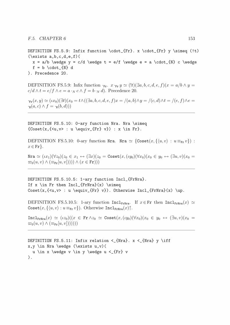
F.5. CHAPTER 6 153
DEFINITION FS.5.9: Infix function \cdot_Fr. x \cdot_Fr y \simeq (!t)
(\exists a,b,c,d,e,f)(
x = a/b \wedge y = c/d \wedge t = e/f \wedge e = a \cdot_N c \wedge
f = b \cdot_N d
). Precedence 20.
DEFINITION FS.5.9: Infix function ·Fr. x ·Fr y ' (!t)(∃a, b, c, d, e, f)(x = a/b ∧ y =c/d ∧ t = e/f ∧ e = a ·N c ∧ f = b ·N d). Precedence 20.
·Fr(x, y) ' (ιx0)(∃t)(x0 = t∧((∃a, b, c, d, e, f)x = /(a, b)∧y = /(c, d)∧t = /(e, f)∧e =·N(a, c) ∧ f = ·N(b, d)))
DEFINITION FS.5.10: 0-ary function Nra. Nra \simeq
Coset(x,<u,v> : u \equiv_Fr v) : x \in Fr.
DEFINITION FS.5.10: 0-ary function Nra. Nra ' Coset(x, 〈u, v〉 : u≡Fr v) :x∈ Fr.
Nra ' (ιx1)(∀z0)(z0 ∈ x1 ↔ (∃x)(z0 = Coset(x, (ιy0)(∀x0)(x0 ∈ y0 ↔ (∃u, v)(x0 =$0(u, v) ∧ (≡Fr[u, v])))) ∧ (x ∈ Fr)))
DEFINITION FS.5.10.5: 1-ary function Incl_FrNra.
If x \in Fr then Incl_FrNra(x) \simeq
Coset(x,<u,v> : u \equiv_Fr v). Otherwise Incl_FrNra(x) \up.
DEFINITION FS.5.10.5: 1-ary function InclFrNra. If x∈ Fr then InclFrNra(x) 'Coset(x, 〈u, v〉 : u≡Fr v). Otherwise InclFrNra(x)↑.
InclFrNra(x) ' (ιz0)((x ∈ Fr∧z0 ' Coset(x, (ιy0)(∀x0)(x0 ∈ y0 ↔ (∃u, v)(x0 =$0(u, v) ∧ (≡Fr[u, v]))))))
DEFINITION FS.5.11: Infix relation <_Nra. x <_Nra y \iff
x,y \in Nra \wedge (\exists u,v)(
u \in x \wedge v \in y \wedge u <_Fr v
).

154 APPENDIX F. DEFINITIONS: FOUNDATIONS – SUPPES
DEFINITION FS.5.11: Infix relation <Nra. x<Nra y ↔ x, y ∈ Nra∧(∃u, v)(u∈x ∧v ∈ y ∧ u<Fr v).
<Nra[x, y] ↔ x ∈ Nra∧y ∈ Nra∧(∃u, v)u ∈ x ∧ v ∈ y ∧<Fr[u, v]
DEFINITION FS.5.12: Infix relation >_Nra. x >_Nra y \iff
x,y \in Nra \wedge (\exists u,v)(
u \in x \wedge v \in y \wedge u >_Fr v
).
DEFINITION FS.5.12: Infix relation >Nra. x>Nra y ↔ x, y ∈ Nra∧(∃u, v)(u∈x ∧v ∈ y ∧ u>Fr v).
>Nra[x, y] ↔ x ∈ Nra∧y ∈ Nra∧(∃u, v)u ∈ x ∧ v ∈ y ∧>Fr[u, v]
DEFINITION FS.5.13: Infix relation \leq_Nra. x \leq_Nra y \iff
x,y \in Nra \wedge
(\exists u,v)(u \in x \wedge v \in y \wedge u \leq_Fr v).
DEFINITION FS.5.13: Infix relation ≤Nra. x≤Nra y ↔ x, y ∈ Nra∧(∃u, v)(u∈x ∧v ∈ y ∧ u≤Fr v).
≤Nra[x, y] ↔ x ∈ Nra∧y ∈ Nra∧(∃u, v)u ∈ x ∧ v ∈ y ∧ ≤Fr[u, v]
DEFINITION FS.5.14: Infix relation \geq_Nra. x \geq_Nra y \iff
x,y \in Nra \wedge
(\exists u,v)(u \in x \wedge v \in y \wedge u \geq_Fr v).
DEFINITION FS.5.14: Infix relation ≥Nra. x≥Nra y ↔ x, y ∈ Nra∧(∃u, v)(u∈x ∧v ∈ y ∧ u≥Fr v).
≥Nra[x, y] ↔ x ∈ Nra∧y ∈ Nra∧(∃u, v)u ∈ x ∧ v ∈ y ∧ ≥Fr[u, v]

F.5. CHAPTER 6 155
DEFINITION FS.5.15: Infix function +_Nra. x +_Nra y \simeq (!z)(
x,y,z \in Nra \wedge (\exists u,v,w)(
u \in x \wedge v \in y \wedge w \in z \wedge
u +_Fr v \equiv_Fr w
)
). Precedence 40.
DEFINITION FS.5.15: Infix function +Nra. x +Nra y ' (!z)(x, y, z ∈ Nra∧(∃u, v, w)(u∈x ∧ v ∈ y ∧ w∈ z ∧ u +Fr v≡Fr w)). Precedence 40.
+Nra(x, y) ' (ιx0)(∃z)(x0 = z ∧ (x ∈ Nra∧y ∈ Nra∧z ∈ Nra∧(∃u, v, w)u ∈ x ∧ v ∈y ∧ w ∈ z ∧ ≡Fr[+Fr(u, v), w]))
DEFINITION FS.5.16: Infix function \cdot_Nra. x \cdot_Nra y \simeq
(!z)(
x,y,z \in Nra \wedge (\exists u,v,w)(
u \in x \wedge v \in y \wedge w \in z \wedge
u \cdot_Fr v \equiv_Fr w
)
). Precedence 20.
DEFINITION FS.5.16: Infix function ·Nra. x ·Nra y ' (!z)(x, y, z ∈ Nra∧(∃u, v, w)(u∈x ∧ v ∈ y ∧ w∈ z ∧ u ·Fr v≡Fr w)). Precedence 20.
·Nra(x, y) ' (ιx0)(∃z)(x0 = z ∧ (x ∈ Nra∧y ∈ Nra∧z ∈ Nra∧(∃u, v, w)u ∈ x ∧ v ∈y ∧ w ∈ z ∧ ≡Fr[·Fr(u, v), w]))
DEFINITION FS.5.17: 0-ary function 0_Nra. 0_Nra \simeq Coset(
0_N/1_N,<x,y> : x \equiv_Fr y
).
DEFINITION FS.5.17: 0-ary function 0Nra. 0Nra ' Coset(0N / 1N, 〈x, y〉 : x≡Fr y).0Nra ' Coset(/(0N, 1N), (ιy0)(∀x0)(x0 ∈ y0 ↔ (∃x, y)(x0 = $0(x, y) ∧ (≡Fr[x, y]))))
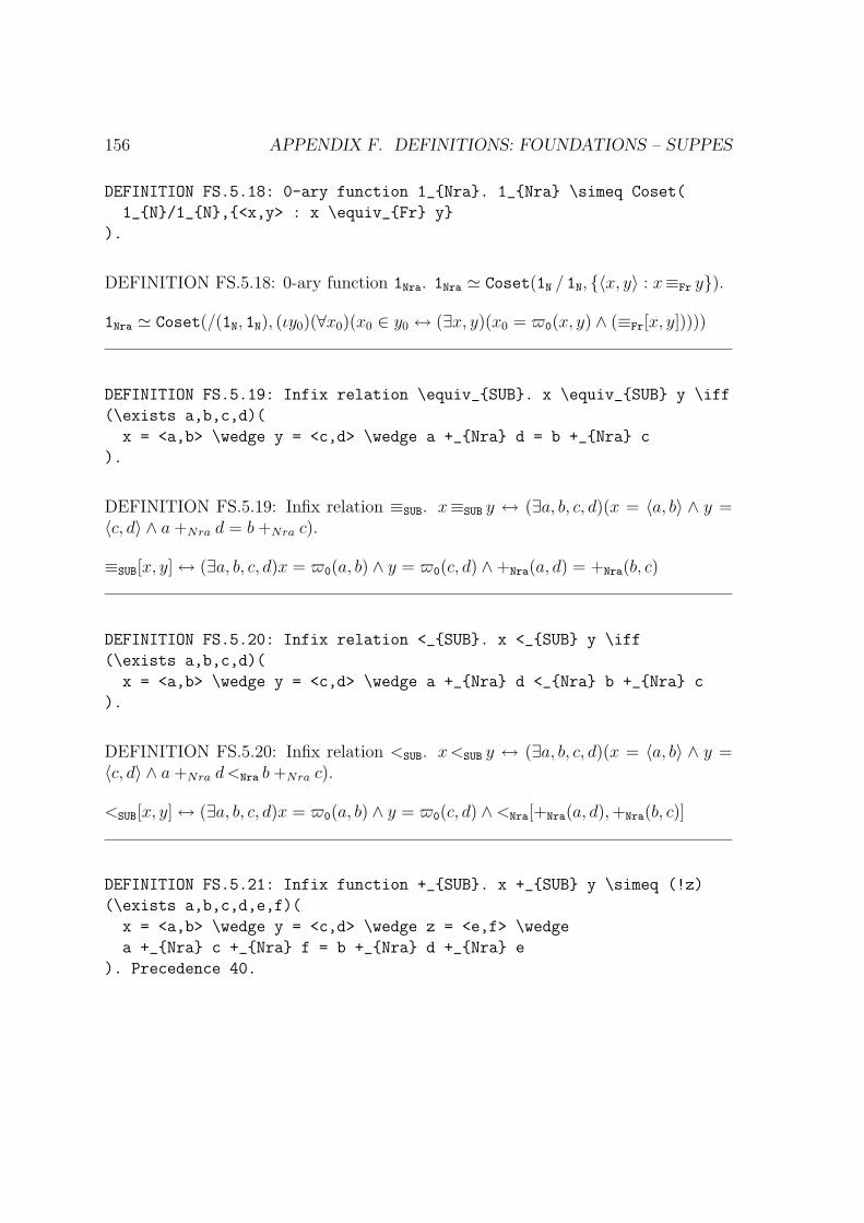
156 APPENDIX F. DEFINITIONS: FOUNDATIONS – SUPPES
DEFINITION FS.5.18: 0-ary function 1_Nra. 1_Nra \simeq Coset(
1_N/1_N,<x,y> : x \equiv_Fr y
).
DEFINITION FS.5.18: 0-ary function 1Nra. 1Nra ' Coset(1N / 1N, 〈x, y〉 : x≡Fr y).
1Nra ' Coset(/(1N, 1N), (ιy0)(∀x0)(x0 ∈ y0 ↔ (∃x, y)(x0 = $0(x, y) ∧ (≡Fr[x, y]))))
DEFINITION FS.5.19: Infix relation \equiv_SUB. x \equiv_SUB y \iff
(\exists a,b,c,d)(
x = <a,b> \wedge y = <c,d> \wedge a +_Nra d = b +_Nra c
).
DEFINITION FS.5.19: Infix relation ≡SUB. x≡SUB y ↔ (∃a, b, c, d)(x = 〈a, b〉 ∧ y =〈c, d〉 ∧ a +Nra d = b +Nra c).
≡SUB[x, y] ↔ (∃a, b, c, d)x = $0(a, b) ∧ y = $0(c, d) ∧+Nra(a, d) = +Nra(b, c)
DEFINITION FS.5.20: Infix relation <_SUB. x <_SUB y \iff
(\exists a,b,c,d)(
x = <a,b> \wedge y = <c,d> \wedge a +_Nra d <_Nra b +_Nra c
).
DEFINITION FS.5.20: Infix relation <SUB. x<SUB y ↔ (∃a, b, c, d)(x = 〈a, b〉 ∧ y =〈c, d〉 ∧ a +Nra d<Nra b +Nra c).
<SUB[x, y] ↔ (∃a, b, c, d)x = $0(a, b) ∧ y = $0(c, d) ∧<Nra[+Nra(a, d), +Nra(b, c)]
DEFINITION FS.5.21: Infix function +_SUB. x +_SUB y \simeq (!z)
(\exists a,b,c,d,e,f)(
x = <a,b> \wedge y = <c,d> \wedge z = <e,f> \wedge
a +_Nra c +_Nra f = b +_Nra d +_Nra e
). Precedence 40.
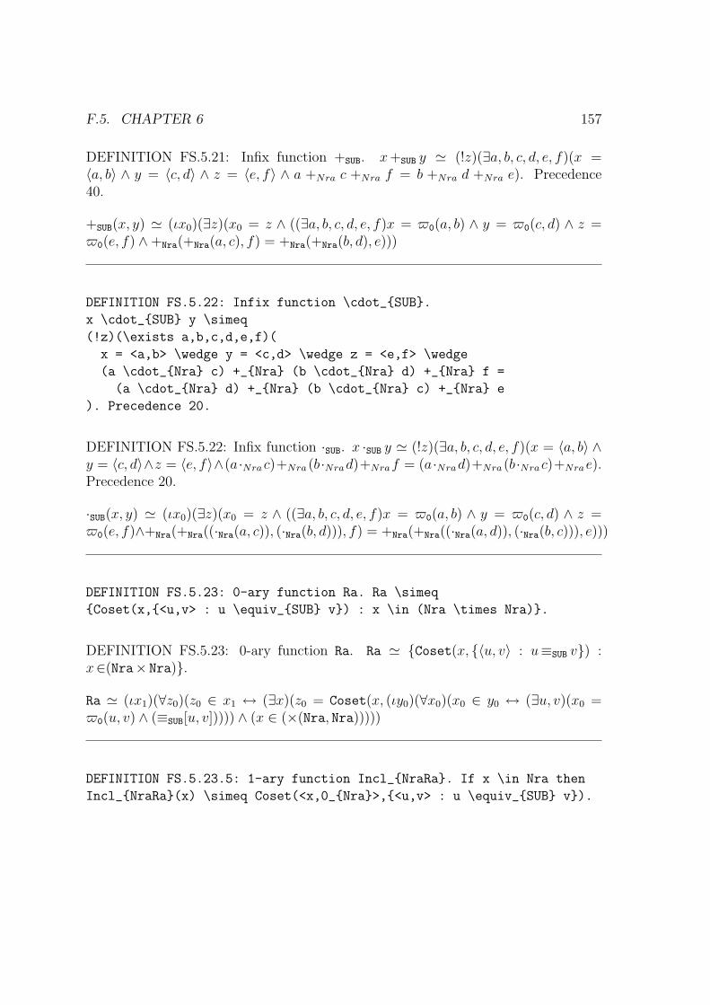
F.5. CHAPTER 6 157
DEFINITION FS.5.21: Infix function +SUB. x +SUB y ' (!z)(∃a, b, c, d, e, f)(x =〈a, b〉 ∧ y = 〈c, d〉 ∧ z = 〈e, f〉 ∧ a +Nra c +Nra f = b +Nra d +Nra e). Precedence40.
+SUB(x, y) ' (ιx0)(∃z)(x0 = z ∧ ((∃a, b, c, d, e, f)x = $0(a, b) ∧ y = $0(c, d) ∧ z =$0(e, f) ∧+Nra(+Nra(a, c), f) = +Nra(+Nra(b, d), e)))
DEFINITION FS.5.22: Infix function \cdot_SUB.
x \cdot_SUB y \simeq
(!z)(\exists a,b,c,d,e,f)(
x = <a,b> \wedge y = <c,d> \wedge z = <e,f> \wedge
(a \cdot_Nra c) +_Nra (b \cdot_Nra d) +_Nra f =
(a \cdot_Nra d) +_Nra (b \cdot_Nra c) +_Nra e
). Precedence 20.
DEFINITION FS.5.22: Infix function ·SUB. x ·SUB y ' (!z)(∃a, b, c, d, e, f)(x = 〈a, b〉 ∧y = 〈c, d〉∧z = 〈e, f〉∧(a ·Nrac)+Nra (b ·Nrad)+Nraf = (a ·Nrad)+Nra (b ·Nrac)+Nrae).Precedence 20.
·SUB(x, y) ' (ιx0)(∃z)(x0 = z ∧ ((∃a, b, c, d, e, f)x = $0(a, b) ∧ y = $0(c, d) ∧ z =$0(e, f)∧+Nra(+Nra((·Nra(a, c)), (·Nra(b, d))), f) = +Nra(+Nra((·Nra(a, d)), (·Nra(b, c))), e)))
DEFINITION FS.5.23: 0-ary function Ra. Ra \simeq
Coset(x,<u,v> : u \equiv_SUB v) : x \in (Nra \times Nra).
DEFINITION FS.5.23: 0-ary function Ra. Ra ' Coset(x, 〈u, v〉 : u≡SUB v) :x∈(Nra× Nra).
Ra ' (ιx1)(∀z0)(z0 ∈ x1 ↔ (∃x)(z0 = Coset(x, (ιy0)(∀x0)(x0 ∈ y0 ↔ (∃u, v)(x0 =$0(u, v) ∧ (≡SUB[u, v])))) ∧ (x ∈ (×(Nra, Nra)))))
DEFINITION FS.5.23.5: 1-ary function Incl_NraRa. If x \in Nra then
Incl_NraRa(x) \simeq Coset(<x,0_Nra>,<u,v> : u \equiv_SUB v).

158 APPENDIX F. DEFINITIONS: FOUNDATIONS – SUPPES
DEFINITION FS.5.23.5: 1-ary function InclNraRa. If x∈ Nra then InclNraRa(x) 'Coset(〈x, 0Nra〉 , 〈u, v〉 : u≡SUB v).InclNraRa(x) ' (ιz0)(x ∈ Nra∧z0 ' Coset($0(x, 0Nra), (ιy0)(∀x0)(x0 ∈ y0 ↔ (∃u, v)(x0 = $0(u, v) ∧ (≡SUB[u, v])))))
DEFINITION FS.5.23.8: 1-ary function Incl_FrRa.
If x \in Fr then Incl_FrRa(x) \simeq Incl_NraRa(Incl_FrNra(x)).
DEFINITION FS.5.23.8: 1-ary function InclFrRa. If x∈ Fr then InclFrRa(x) 'InclNraRa(InclFrNra(x)).
InclFrRa(x) ' (ιx0)(x ∈ Fr∧x0 ' InclNraRa(InclFrNra(x)))
DEFINITION FS.5.23.A: 0-ary function \mathbbQ. \mathbbQ \simeq Ra.
DEFINITION FS.5.23.A: 0-ary function Q. Q ' Ra.
Q ' Ra
DEFINITION FS.5.24: Infix relation <_Ra. x <_Ra y \iff
(\exists z,w)(
x,y \in Ra \wedge z \in x \wedge w \in y \wedge z <_SUB w
).
DEFINITION FS.5.24: Infix relation <Ra. x<Ra y ↔ (∃z, w)(x, y ∈ Ra∧z ∈x∧w∈ y∧z <SUB w).
<Ra[x, y] ↔ (∃z, w)x ∈ Ra∧y ∈ Ra∧z ∈ x ∧ w ∈ y ∧<SUB[z, w]
DEFINITION FS.5.25: Infix function +_Ra. x +_Ra y \simeq (!z)(
x,y,z \in Ra \wedge (\exists a,b,c)(
a \in x \wedge b \in y \wedge c \in z \wedge a +_SUB b = c
)
). Precedence 40.
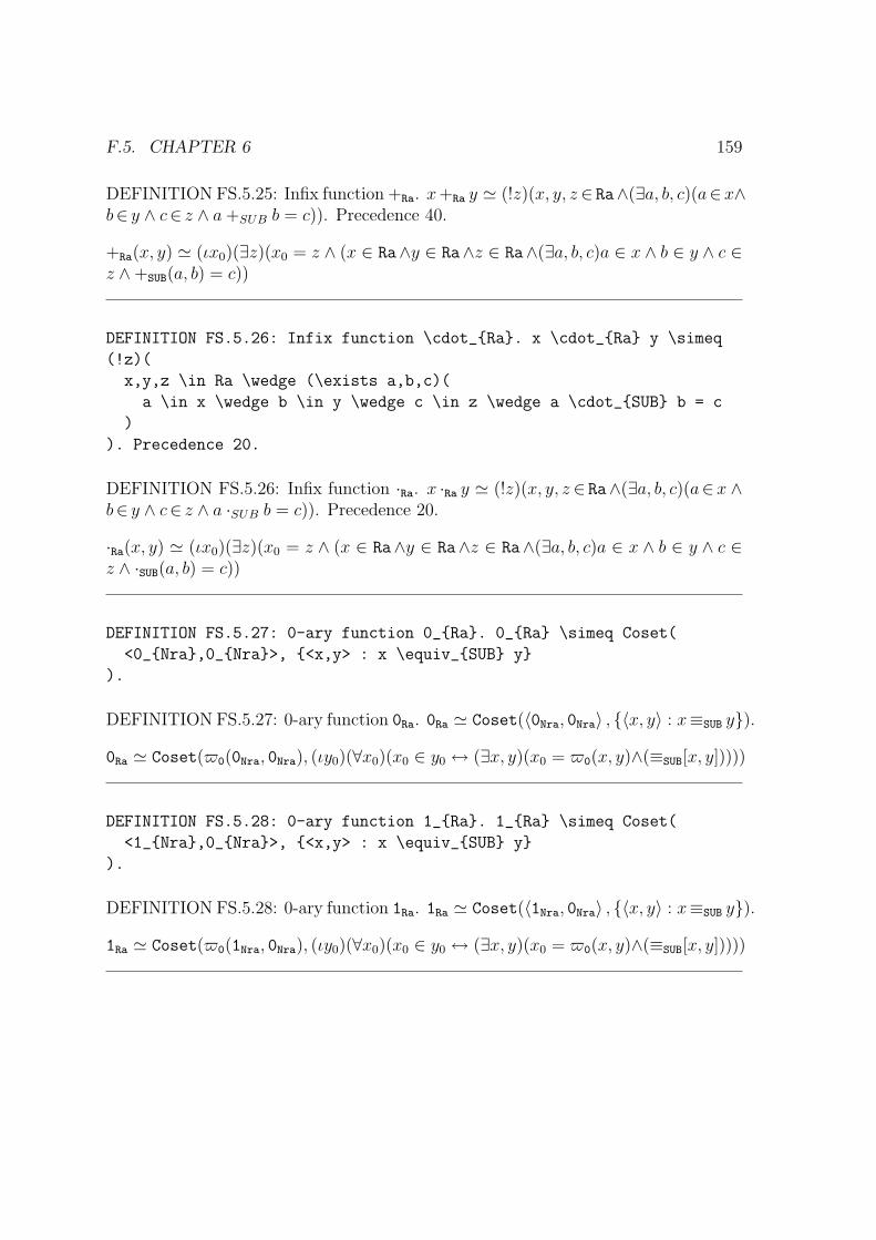
F.5. CHAPTER 6 159
DEFINITION FS.5.25: Infix function +Ra. x +Ra y ' (!z)(x, y, z ∈ Ra∧(∃a, b, c)(a∈x∧b∈ y ∧ c∈ z ∧ a +SUB b = c)). Precedence 40.
+Ra(x, y) ' (ιx0)(∃z)(x0 = z ∧ (x ∈ Ra∧y ∈ Ra∧z ∈ Ra∧(∃a, b, c)a ∈ x ∧ b ∈ y ∧ c ∈z ∧+SUB(a, b) = c))
DEFINITION FS.5.26: Infix function \cdot_Ra. x \cdot_Ra y \simeq
(!z)(
x,y,z \in Ra \wedge (\exists a,b,c)(
a \in x \wedge b \in y \wedge c \in z \wedge a \cdot_SUB b = c
)
). Precedence 20.
DEFINITION FS.5.26: Infix function ·Ra. x ·Ra y ' (!z)(x, y, z ∈ Ra∧(∃a, b, c)(a∈x ∧b∈ y ∧ c∈ z ∧ a ·SUB b = c)). Precedence 20.
·Ra(x, y) ' (ιx0)(∃z)(x0 = z ∧ (x ∈ Ra∧y ∈ Ra∧z ∈ Ra∧(∃a, b, c)a ∈ x ∧ b ∈ y ∧ c ∈z ∧ ·SUB(a, b) = c))
DEFINITION FS.5.27: 0-ary function 0_Ra. 0_Ra \simeq Coset(
<0_Nra,0_Nra>, <x,y> : x \equiv_SUB y
).
DEFINITION FS.5.27: 0-ary function 0Ra. 0Ra ' Coset(〈0Nra, 0Nra〉 , 〈x, y〉 : x≡SUB y).0Ra ' Coset($0(0Nra, 0Nra), (ιy0)(∀x0)(x0 ∈ y0 ↔ (∃x, y)(x0 = $0(x, y)∧(≡SUB[x, y]))))
DEFINITION FS.5.28: 0-ary function 1_Ra. 1_Ra \simeq Coset(
<1_Nra,0_Nra>, <x,y> : x \equiv_SUB y
).
DEFINITION FS.5.28: 0-ary function 1Ra. 1Ra ' Coset(〈1Nra, 0Nra〉 , 〈x, y〉 : x≡SUB y).1Ra ' Coset($0(1Nra, 0Nra), (ιy0)(∀x0)(x0 ∈ y0 ↔ (∃x, y)(x0 = $0(x, y)∧(≡SUB[x, y]))))

160 APPENDIX F. DEFINITIONS: FOUNDATIONS – SUPPES
DEFINITION FS.5.29: Infix relation >_Ra. x >_Ra y \iff y <_Ra x.
DEFINITION FS.5.29: Infix relation >Ra. x>Ra y ↔ y <Ra x.
>Ra[x, y] ↔ <Ra[y, x]
DEFINITION FS.5.30: Infix relation \leq_Ra. x \leq_Ra y \iff
x <_Ra y \vee x = y.
DEFINITION FS.5.30: Infix relation ≤Ra. x≤Ra y ↔ x <Ra y ∨ x = y.
≤Ra[x, y] ↔ <Ra[x, y] ∨ x = y
DEFINITION FS.5.31: Infix relation \geq_Ra. x \geq_Ra y \iff
x >_Ra y \vee x = y.
DEFINITION FS.5.31: Infix relation ≥Ra. x≥Ra y ↔ x >Ra y ∨ x = y.
≥Ra[x, y] ↔ >Ra[x, y] ∨ x = y
DEFINITION FS.5.32: Infix function -_Ra. x -_Ra y \simeq
(!z)(x = y +_Ra z). Precedence 60.
DEFINITION FS.5.32: Infix function −Ra. x−Ra y ' (!z)(x = y +Ra z). Precedence60.
−Ra(x, y) ' (ιx0)(∃z)(x0 = z ∧ (x = +Ra(y, z)))
DEFINITION FS.5.33: 1-ary function Av_Ra. Av_Ra(x) \simeq
(!y \in Ra)(
(x \geq_Ra 0_Ra \implies y = x) \wedge
(x <_Ra 0_Ra \implies y = 0_Ra -_Ra x)
).
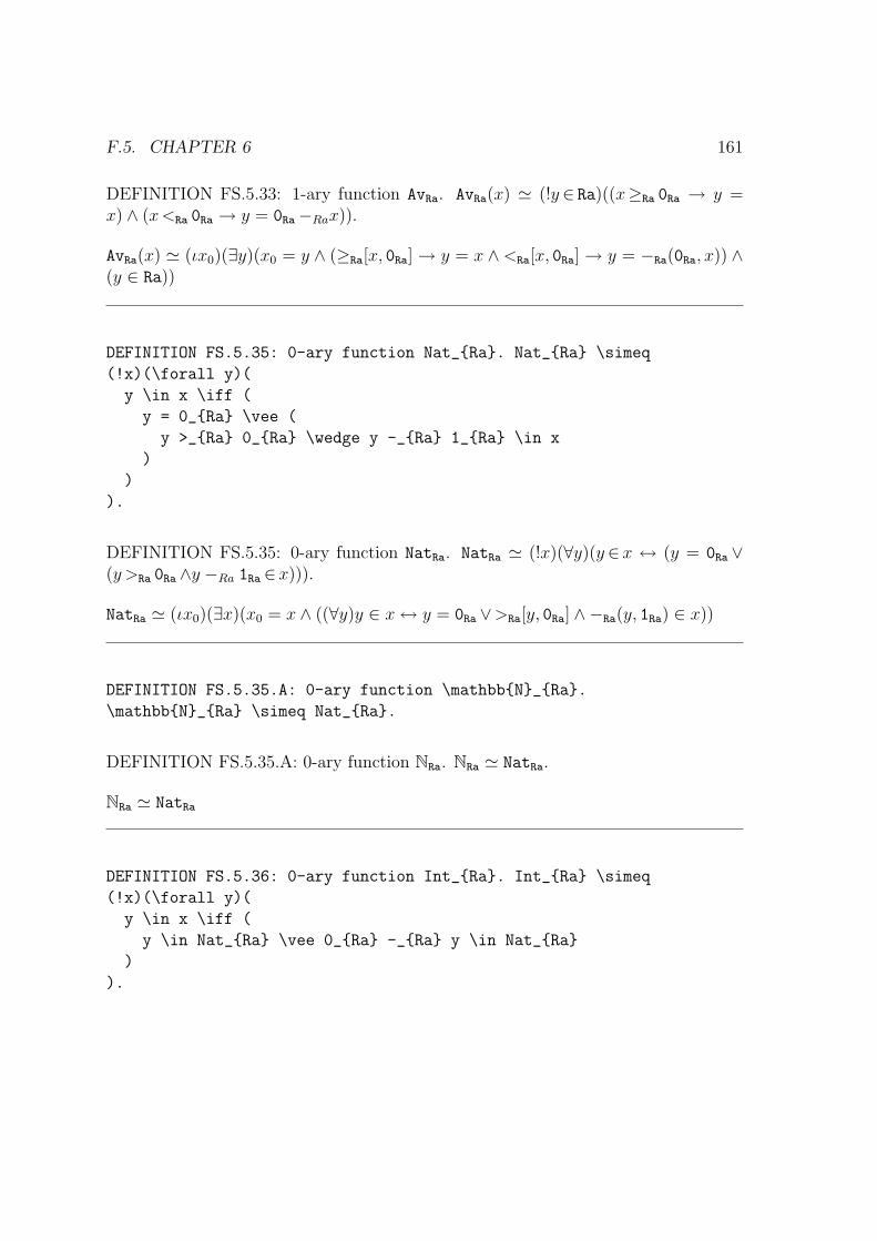
F.5. CHAPTER 6 161
DEFINITION FS.5.33: 1-ary function AvRa. AvRa(x) ' (!y ∈ Ra)((x≥Ra 0Ra → y =x) ∧ (x<Ra 0Ra → y = 0Ra−Rax)).
AvRa(x) ' (ιx0)(∃y)(x0 = y ∧ (≥Ra[x, 0Ra] → y = x ∧ <Ra[x, 0Ra] → y = −Ra(0Ra, x)) ∧(y ∈ Ra))
DEFINITION FS.5.35: 0-ary function Nat_Ra. Nat_Ra \simeq
(!x)(\forall y)(
y \in x \iff (
y = 0_Ra \vee (
y >_Ra 0_Ra \wedge y -_Ra 1_Ra \in x
)
)
).
DEFINITION FS.5.35: 0-ary function NatRa. NatRa ' (!x)(∀y)(y ∈x ↔ (y = 0Ra ∨(y >Ra 0Ra ∧y −Ra 1Ra ∈x))).
NatRa ' (ιx0)(∃x)(x0 = x ∧ ((∀y)y ∈ x ↔ y = 0Ra ∨>Ra[y, 0Ra] ∧ −Ra(y, 1Ra) ∈ x))
DEFINITION FS.5.35.A: 0-ary function \mathbbN_Ra.
\mathbbN_Ra \simeq Nat_Ra.
DEFINITION FS.5.35.A: 0-ary function NRa. NRa ' NatRa.
NRa ' NatRa
DEFINITION FS.5.36: 0-ary function Int_Ra. Int_Ra \simeq
(!x)(\forall y)(
y \in x \iff (
y \in Nat_Ra \vee 0_Ra -_Ra y \in Nat_Ra
)
).

162 APPENDIX F. DEFINITIONS: FOUNDATIONS – SUPPES
DEFINITION FS.5.36: 0-ary function IntRa. IntRa ' (!x)(∀y)(y ∈x ↔ (y ∈ NatRa ∨0Ra−Ray ∈ NatRa)).
IntRa ' (ιx0)(∃x)(x0 = x ∧ ((∀y)y ∈ x ↔ y ∈ NatRa ∨−Ra(0Ra, y) ∈ NatRa))
DEFINITION FS.5.36.A: 0-ary function \mathbbZ_Ra.
\mathbbZ_Ra \simeq Int_Ra.
DEFINITION FS.5.36.A: 0-ary function ZRa. ZRa ' IntRa.
ZRa ' IntRa
DEFINITION FS.5.37: 0-ary function Seq_Ra.
Seq_Ra \simeq Maps(\omega,Ra).
DEFINITION FS.5.37: 0-ary function SeqRa. SeqRa ' Maps(ω, Ra).
SeqRa ' Maps(ω, Ra)
DEFINITION FS.5.38: Infix function +_SeqRa.
x +_SeqRa y \simeq (!z)(
x,y,z \in Seq_Ra \wedge
(\forall n \in \omega)(z(n) = x(n) +_Ra y(n))
). Precedence 40.
DEFINITION FS.5.38: Infix function +SeqRa. x +SeqRa y ' (!z)(x, y, z ∈ SeqRa ∧(∀n∈ω)(z(n) = x(n) +Ra y(n))). Precedence 40.
+SeqRa(x, y) ' (ιy0)(∃z)(y0 = z ∧ (x ∈ SeqRa ∧y ∈ SeqRa ∧z ∈ SeqRa ∧(∀n)(n ∈ ω →(ιx0)($0(n, x0) ∈ z) = +Ra((ιx0)($0(n, x0) ∈ x), (ιx0)($0(n, x0) ∈ y)))))

F.5. CHAPTER 6 163
DEFINITION FS.5.39: Infix function \cdot_SeqRa.
x \cdot_SeqRa y \simeq (!z)(
x,y,z \in Seq_Ra \wedge
(\forall n \in \omega)(z(n) = x(n) \cdot_Ra y(n))
). Precedence 20.
DEFINITION FS.5.39: Infix function ·SeqRa. x ·SeqRa y ' (!z)(x, y, z ∈ SeqRa ∧(∀n∈ω)(z(n) = x(n) ·Ra y(n))). Precedence 20.
·SeqRa(x, y) ' (ιy0)(∃z)(y0 = z ∧ (x ∈ SeqRa ∧y ∈ SeqRa ∧z ∈ SeqRa ∧(∀n)(n ∈ ω →(ιx0)($0(n, x0) ∈ z) = ·Ra((ιx0)($0(n, x0) ∈ x), (ιx0)($0(n, x0) ∈ y)))))
DEFINITION FS.5.40: Infix relation <_N. x <_N y \iff
x,y \in \omega \wedge x <_O y.
DEFINITION FS.5.40: Infix relation <N. x<N y ↔ x, y ∈ω ∧x<O y.
<N[x, y] ↔ x ∈ ω ∧y ∈ ω ∧<O[x, y]
DEFINITION FS.5.41: Infix relation >_N. x >_N y \iff
x,y \in \omega \wedge x >_O y.
DEFINITION FS.5.41: Infix relation >N. x>N y ↔ x, y ∈ω ∧x>O y.
>N[x, y] ↔ x ∈ ω ∧y ∈ ω ∧>O[x, y]
DEFINITION FS.5.42: Infix relation \leq_N. x \leq_N y \iff
x <_N y \vee x = y.
DEFINITION FS.5.42: Infix relation ≤N. x≤N y ↔ x<N y ∨ x = y.
≤N[x, y] ↔ <N[x, y] ∨ x = y

164 APPENDIX F. DEFINITIONS: FOUNDATIONS – SUPPES
DEFINITION FS.5.43: Infix relation \geq_N. x \geq_N y \iff
x >_N y \vee x = y.
DEFINITION FS.5.43: Infix relation ≥N. x≥N y ↔ x>N y ∨ x = y.
≥N[x, y] ↔ >N[x, y] ∨ x = y
DEFINITION FS.5.44: 0-ary function Cseq_Ra. Cseq_Ra \simeq
x \in Seq_Ra : (\forall \veps >_Ra 0_Ra)(\exists n \in \omega)
(\forall m,r >_N n)(
Av_Ra(x(m) -_Ra x(r)) <_Ra \veps
)
.
DEFINITION FS.5.44: 0-ary function CseqRa. CseqRa ' x∈ SeqRa : (∀ε>Ra 0Ra)(∃n∈ω)(∀m, r >N n)(AvRa(x(m)−Ra x(r)) <Ra ε).
CseqRa ' (ιz0)(∀y0)(y0 ∈ z0 ↔ (∃x)(y0 = x∧ ((∀ε)(>Ra[ε, 0Ra] → (∃n)(n ∈ ω ∧(∀m, r)(>N[m, n]∧>N[r, n] → <Ra[AvRa(−Ra((ιx0)($0(m,x0) ∈ x), (ιx0)($0(r, x0) ∈ x))), ε]))))∧(x ∈ SeqRa)))
DEFINITION FS.5.45: Infix relation \equiv_CseqRa.
x \equiv_CseqRa y \iff
(\forall \veps >_Ra 0_Ra)(\exists n \in \omega)
(\forall m >_N n)(
Av_Ra(x(m) -_Ra y(m)) <_Ra \veps
).
DEFINITION FS.5.45: Infix relation ≡CseqRa. x≡CseqRa y ↔ (∀ε>Ra 0Ra)(∃n∈ω)(∀m>N n)(AvRa(x(m)−Ra y(m)) <Ra ε).
≡CseqRa[x, y] ↔ (∀ε)(>Ra[ε, 0Ra] → (∃n)(n ∈ ω ∧(∀m)(>N[m,n] →<Ra[AvRa(−Ra((ιx0)($0(m,x0) ∈ x), (ιx0)($0(m,x0) ∈ y))), ε])))
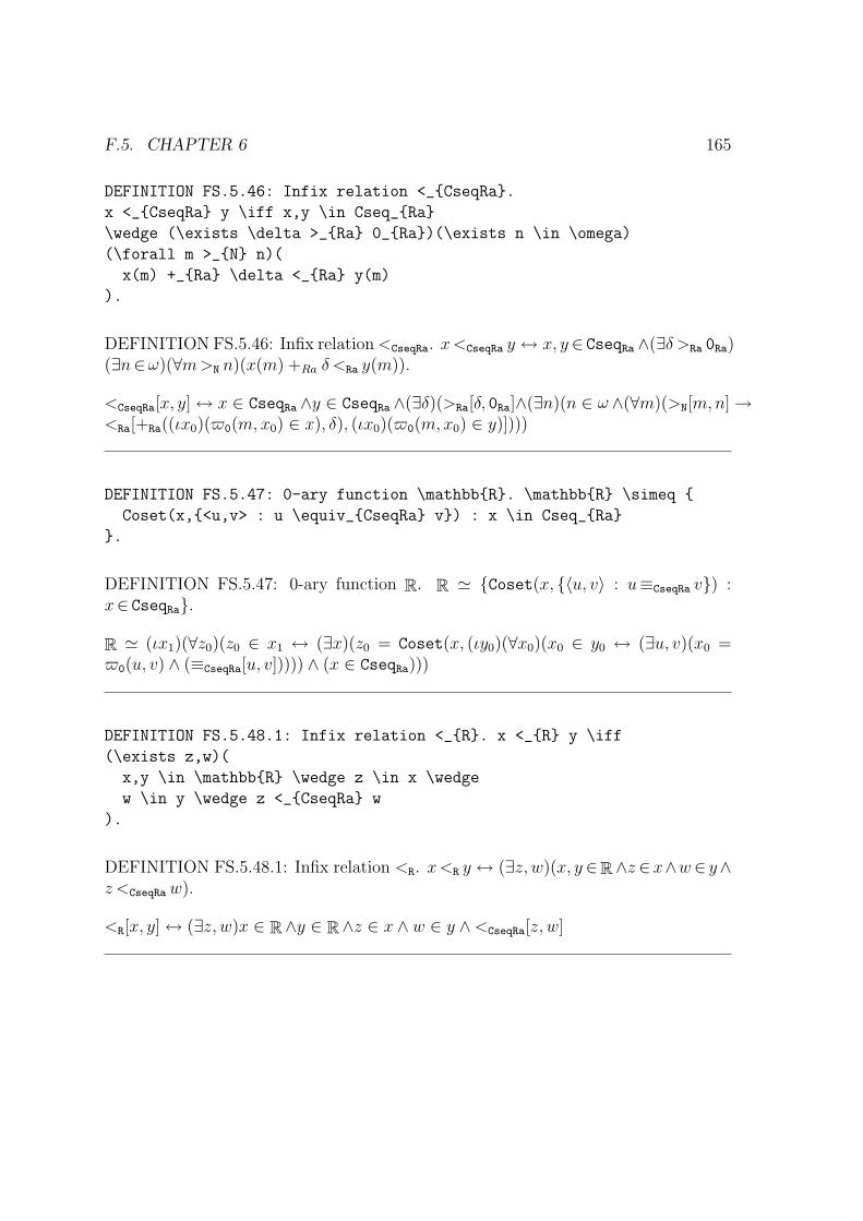
F.5. CHAPTER 6 165
DEFINITION FS.5.46: Infix relation <_CseqRa.
x <_CseqRa y \iff x,y \in Cseq_Ra
\wedge (\exists \delta >_Ra 0_Ra)(\exists n \in \omega)
(\forall m >_N n)(
x(m) +_Ra \delta <_Ra y(m)
).
DEFINITION FS.5.46: Infix relation <CseqRa. x<CseqRa y ↔ x, y ∈ CseqRa ∧(∃δ >Ra 0Ra)(∃n∈ω)(∀m>N n)(x(m) +Ra δ <Ra y(m)).
<CseqRa[x, y] ↔ x ∈ CseqRa ∧y ∈ CseqRa ∧(∃δ)(>Ra[δ, 0Ra]∧(∃n)(n ∈ ω ∧(∀m)(>N[m,n] →<Ra[+Ra((ιx0)($0(m, x0) ∈ x), δ), (ιx0)($0(m,x0) ∈ y)])))
DEFINITION FS.5.47: 0-ary function \mathbbR. \mathbbR \simeq
Coset(x,<u,v> : u \equiv_CseqRa v) : x \in Cseq_Ra
.
DEFINITION FS.5.47: 0-ary function R. R ' Coset(x, 〈u, v〉 : u≡CseqRa v) :x∈ CseqRa.
R ' (ιx1)(∀z0)(z0 ∈ x1 ↔ (∃x)(z0 = Coset(x, (ιy0)(∀x0)(x0 ∈ y0 ↔ (∃u, v)(x0 =$0(u, v) ∧ (≡CseqRa[u, v])))) ∧ (x ∈ CseqRa)))
DEFINITION FS.5.48.1: Infix relation <_R. x <_R y \iff
(\exists z,w)(
x,y \in \mathbbR \wedge z \in x \wedge
w \in y \wedge z <_CseqRa w
).
DEFINITION FS.5.48.1: Infix relation <R. x<R y ↔ (∃z, w)(x, y ∈R∧z ∈x∧w∈ y∧z <CseqRa w).
<R[x, y] ↔ (∃z, w)x ∈ R∧y ∈ R∧z ∈ x ∧ w ∈ y ∧<CseqRa[z, w]
166 APPENDIX F. DEFINITIONS: FOUNDATIONS – SUPPES
DEFINITION FS.5.48.2: Infix relation >_R. x >_R y \iff y <_R x.
DEFINITION FS.5.48.2: Infix relation >R. x>R y ↔ y <R x.
>R[x, y] ↔ <R[y, x]
DEFINITION FS.5.48.3: Infix relation \leq_R. x \leq_R y \iff
x <_R y \vee x = y.
DEFINITION FS.5.48.3: Infix relation ≤R. x≤R y ↔ x<R y ∨ x = y.
≤R[x, y] ↔ <R[x, y] ∨ x = y
DEFINITION FS.5.48.4: Infix relation \geq_R. x \geq_R y \iff
x >_R y \vee x = y.
DEFINITION FS.5.48.4: Infix relation ≥R. x≥R y ↔ x>R y ∨ x = y.
≥R[x, y] ↔ >R[x, y] ∨ x = y
DEFINITION FS.5.49: Infix function +_R. x +_R y \simeq (!z)(
x,y,z \in \mathbbR \wedge (\exists a,b,c)(
a \in x \wedge b \in y \wedge c \in z \wedge
a +_SeqRa b \equiv_CseqRa c
)
). Precedence 40.
DEFINITION FS.5.49: Infix function +R. x +R y ' (!z)(x, y, z ∈R∧(∃a, b, c)(a∈x ∧b∈ y ∧ c∈ z ∧ a +SeqRa b≡CseqRa c)). Precedence 40.
+R(x, y) ' (ιx0)(∃z)(x0 = z ∧ (x ∈ R∧y ∈ R∧z ∈ R∧(∃a, b, c)a ∈ x ∧ b ∈ y ∧ c ∈z ∧ ≡CseqRa[+SeqRa(a, b), c]))

F.5. CHAPTER 6 167
DEFINITION FS.5.49.A: Infix function -_R. x -_R y \simeq
(!z)(x = y +_R z). Precedence 60.
DEFINITION FS.5.49.A: Infix function −R. x−R y ' (!z)(x = y +R z). Precedence60.
−R(x, y) ' (ιx0)(∃z)(x0 = z ∧ (x = +R(y, z)))
DEFINITION FS.5.50: Infix function \cdot_R.
x \cdot_R y \simeq (!z)(
x,y,z \in \mathbbR \wedge (\exists a,b,c)(
a \in x \wedge b \in y \wedge c \in z \wedge
a \cdot_SeqRa b \equiv_CseqRa c
)
). Precedence 20.
DEFINITION FS.5.50: Infix function ·R. x ·R y ' (!z)(x, y, z ∈R∧(∃a, b, c)(a∈x ∧b∈ y ∧ c∈ z ∧ a ·SeqRa b≡CseqRa c)). Precedence 20.
·R(x, y) ' (ιx0)(∃z)(x0 = z ∧ (x ∈ R∧y ∈ R∧z ∈ R∧(∃a, b, c)a ∈ x ∧ b ∈ y ∧ c ∈z ∧ ≡CseqRa[·SeqRa(a, b), c]))
DEFINITION FS.5.51: 0-ary function 0_R.
0_R \simeq (!x \in \mathbbR)(
(\exists w \in x)(\forall n \in \omega)(w(n) = 0_Ra)
).
DEFINITION FS.5.51: 0-ary function 0R. 0R ' (!x∈R)((∃w∈x)(∀n∈ω)(w(n) =0Ra)).
0R ' (ιy0)(∃x)(y0 = x ∧ ((∃w)(w ∈ x ∧ (∀n)(n ∈ ω → (ιx0)($0(n, x0) ∈ w) =0Ra))) ∧ (x ∈ R))
168 APPENDIX F. DEFINITIONS: FOUNDATIONS – SUPPES
DEFINITION FS.5.52: 0-ary function 1_R.
1_R \simeq (!x \in \mathbbR)(
(\exists w \in x)(\forall n \in \omega)(w(n) = 1_Ra)
).
DEFINITION FS.5.52: 0-ary function 1R. 1R ' (!x∈R)((∃w∈x)(∀n∈ω)(w(n) =1Ra)).
1R ' (ιy0)(∃x)(y0 = x ∧ ((∃w)(w ∈ x ∧ (∀n)(n ∈ ω → (ιx0)($0(n, x0) ∈ w) =1Ra))) ∧ (x ∈ R))
DEFINITION FS.5.53: 1-ary function Av_R.
Av_R(x) \simeq (!y \in \mathbbR)(
(x \geq_R 0_R \implies y = x) \wedge
(x <_R 0_R \implies y = 0_R -_R x)
).
DEFINITION FS.5.53: 1-ary function AvR. AvR(x) ' (!y ∈R)((x≥R 0R → y = x) ∧(x<R 0R → y = 0R−Rx)).
AvR(x) ' (ιx0)(∃y)(x0 = y∧(≥R[x, 0R] → y = x∧<R[x, 0R] → y = −R(0R, x))∧(y ∈ R))
DEFINITION FS.5.53.A: 1-ary function Id_R.
Id_R(x) \simeq (!y \in \mathbbR)(
(\exists w \in y)(\forall n \in \omega)(w(n) = x)
).
DEFINITION FS.5.53.A: 1-ary function IdR. IdR(x) ' (!y ∈R)((∃w∈ y)(∀n∈ω)(w(n) =x)).
IdR(x) ' (ιy0)(∃y)(y0 = y ∧ ((∃w)(w ∈ y ∧ (∀n)(n ∈ ω → (ιx0)($0(n, x0) ∈ w) =x))) ∧ (y ∈ R))
DEFINITION FS.5.53.B: 1-ary function Incl_NraR.
If x \in Nra then Incl_NraR(x) \simeq Id_R(Incl_NraRa(x)).
F.5. CHAPTER 6 169
DEFINITION FS.5.53.B: 1-ary function InclNraR. If x∈ Nra then InclNraR(x) 'IdR(InclNraRa(x)).
InclNraR(x) ' (ιx0)(x ∈ Nra∧x0 ' IdR(InclNraRa(x)))
DEFINITION FS.5.53.C: 1-ary function Incl_FrR.
If x \in Fr then Incl_FrR(x) \simeq Id_R(Incl_FrRa(x)).
DEFINITION FS.5.53.C: 1-ary function InclFrR. If x∈ Fr then InclFrR(x) 'IdR(InclFrRa(x)).
InclFrR(x) ' (ιx0)(x ∈ Fr∧x0 ' IdR(InclFrRa(x)))
DEFINITION FS.5.54: 0-ary function Ra_R.
Ra_R \simeq Id_R(x) : x \in Ra.
DEFINITION FS.5.54: 0-ary function RaR. RaR ' IdR(x) : x∈ Ra.
RaR ' (ιy0)(∀x0)(x0 ∈ y0 ↔ (∃x)(x0 = IdR(x) ∧ (x ∈ Ra)))
DEFINITION FS.5.55: 0-ary function Seq_R.
Seq_R \simeq Maps(\omega,\mathbbR).
DEFINITION FS.5.55: 0-ary function SeqR. SeqR ' Maps(ω,R).
SeqR ' Maps(ω,R)
DEFINITION FS.5.56: 0-ary function Cseq_R. Cseq_R \simeq
x \in Seq_R : (\forall \veps >_Ra 0_Ra)(\exists n \in \omega)
(\forall m,r >_N n)(
Av_R(x(m) -_R x(r)) <_R \veps
)
.
170 APPENDIX F. DEFINITIONS: FOUNDATIONS – SUPPES
DEFINITION FS.5.56: 0-ary function CseqR. CseqR ' x∈ SeqR : (∀ε >Ra 0Ra)(∃n∈ω)(∀m, r >N n)(AvR(x(m)−R x(r)) <R ε).
CseqR ' (ιz0)(∀y0)(y0 ∈ z0 ↔ (∃x)(y0 = x ∧ ((∀ε)(>Ra[ε, 0Ra] → (∃n)(n ∈ ω ∧(∀m, r)(>N[m, n]∧>N[r, n] → <R[AvR(−R((ιx0)($0(m,x0) ∈ x), (ιx0)($0(r, x0) ∈ x))), ε]))))∧(x ∈ SeqR)))
DEFINITION FS.5.57: 1-ary function Lim.
If x \in Seq_R then Lim(x) \simeq
(!y \in \mathbbR)(
(\forall \veps >_R 0_R)(\exists n \in \omega)
(\forall m >_N n)(
Av_R(x(m) -_R y) <_R \veps
)
).
DEFINITION FS.5.57: 1-ary function Lim. If x∈ SeqR then Lim(x) '(!y ∈R)((∀ε>R 0R)(∃n∈ω)(∀m>N n)(AvR(x(m)−R y) <R ε)).
Lim(x) ' (ιz0)(x ∈ SeqR ∧z0 ' (ιy0)(∃y)(y0 = y ∧ ((∀ε)(>R[ε, 0R] → (∃n)(n ∈ω ∧(∀m)(>N[m,n] → <R[AvR(−R((ιx0)($0(m,x0) ∈ x), y)), ε])))) ∧ (y ∈ R)))
DEFINITION FS.5.58: 2-ary relation UB_R.
UB_R[x,A] \iff x \in \mathbbR \wedge
A \subseteq \mathbbR \wedge (\forall y \in A)(y \leq_R x).
DEFINITION FS.5.58: 2-ary relation UBR. UBR[x,A] ↔ x∈R∧A⊆R∧(∀y ∈A)(y≤R x).
UBR[x,A] ↔ x ∈ R∧⊆[A,R] ∧ (∀y)(y ∈ A → ≤R[y, x])
DEFINITION FS.5.59: 1-ary function Min_R.
If A \subseteq \mathbbR then
Min_R(A) \simeq (!x \in A)(
(\forall y \in A)(\neg(y <_R x))
).

F.5. CHAPTER 6 171
DEFINITION FS.5.59: 1-ary function MinR. If A⊆R then MinR(A) ' (!x∈A)((∀y ∈A)(¬(y <R x))).
MinR(A) ' (ιy0)(⊆[A,R]∧y0 ' (ιx0)(∃x)(x0 = x∧((∀y)(y ∈ A → ¬(<R[y, x])))∧(x ∈A)))
DEFINITION FS.5.59.5: 1-ary function Max_R.
If A \subseteq \mathbbR then
Max_R(A) \simeq (!x \in A)(
(\forall y \in A)(\neg(x <_R y))
).
DEFINITION FS.5.59.5: 1-ary function MaxR. If A⊆R then MaxR(A) ' (!x∈A)((∀y ∈A)(¬(x<R y))).
MaxR(A) ' (ιy0)(⊆[A,R]∧y0 ' (ιx0)(∃x)(x0 = x∧((∀y)(y ∈ A → ¬(<R[x, y])))∧(x ∈A)))
DEFINITION FS.5.60: 1-ary function Lub_R.
If A \subseteq \mathbbR then
Lub_R(A) \simeq Min_R(x : UB_R[x,A]).
DEFINITION FS.5.60: 1-ary function LubR. If A⊆R then LubR(A) ' MinR(x :UBR[x,A]).
LubR(A) ' (ιz0)(⊆[A,R]∧z0 ' MinR((ιy0)(∀x0)(x0 ∈ y0 ↔ (∃x)(x0 = x∧(UBR[x,A])))))
DEFINITION FS.5.61.pre: 1-ary function Finitesumset_R.
If (\exists n \in \omega)
(FCN[f,n,\mathbbR]) then Finitesumset_R(f) \simeq (!x)(
(\forall m \in \omega)(
(m <_N n \implies (
x(0_N) = 0_R \wedge
x(Suc(m)) = x(m) +_R f(Suc(m))

172 APPENDIX F. DEFINITIONS: FOUNDATIONS – SUPPES
)
) \wedge
(m \geq_N n \implies x(Suc(m)) = 0_R)
) \wedge
(\forall m)(
x(m) \dn \iff m \in \omega
)
).
DEFINITION FS.5.61.pre: 1-ary function FinitesumsetR. If (∃n∈ω)(FCN[f, n,R])then FinitesumsetR(f) ' (!x)((∀m∈ω)((m<N n → (x(0N) = 0R ∧x(Suc(m)) =x(m) +R f(Suc(m)))) ∧ (m≥N n → x(Suc(m)) = 0R)) ∧ (∀m)(x(m)↓ ↔ m∈ω)).
FinitesumsetR(f) ' (ιz0)((∃n)(n ∈ ω ∧ FCN[f, n,R]) ∧ z0 ' (ιy0)(∃x)(y0 = x ∧((∀m)(m ∈ ω → <N[m, n] → (ιx0)($0(0N, x0) ∈ x) = 0R ∧(ιx0)($0(Suc(m), x0) ∈x) = +R((ιx0)($0(m,x0) ∈ x), (ιx0)($0(Suc(m), x0) ∈ f)) ∧ ≥N[m,n] → (ιx0)($0(Suc(m), x0) ∈ x) = 0R) ∧ (∀m)(ιx0)($0(m,x0) ∈ x)↓ ↔ m ∈ ω)))
DEFINITION FS.5.61: 1-ary function Finitesum_R.
If (\exists n \in \omega)
(FCN[f,n,\mathbbR]) then Finitesum_R(f) \simeq
(!r \in \mathbbR)(<Dom(f),r> \in Finitesumset_R(f)).
DEFINITION FS.5.61: 1-ary function FinitesumR. If (∃n∈ω)(FCN[f, n,R]) thenFinitesumR(f) ' (!r∈R)(〈Dom(f), r〉 ∈ FinitesumsetR(f)).
FinitesumR(f) ' (ιy0)((∃n)(n ∈ ω ∧ FCN[f, n,R]) ∧ y0 ' (ιx0)(∃r)(x0 = r∧($0(Dom(f), r) ∈ FinitesumsetR(f)) ∧ (r ∈ R)))
DEFINITION FS.5.62: 1-ary function Sqrt_R.
If r \in \mathbbR then Sqrt_R(r)
\simeq (!y \in \mathbbR)(
y \geq_R 0_R \wedge y \cdot_R y = r
).

F.5. CHAPTER 6 173
DEFINITION FS.5.62: 1-ary function SqrtR. If r∈R then SqrtR(r) ' (!y ∈R)(y≥R 0R ∧y ·R y = r).
SqrtR(r) ' (ιy0)(r ∈ R∧y0 ' (ιx0)(∃y)(x0 = y ∧ (≥R[y, 0R] ∧ ·R(y, y) = r) ∧ (y ∈ R)))
DEFINITION FS.5.63: 1-ary function Sup_R. Sup_R(A) \simeq (!s)(
SUP[s,<x,y>: x <_R y,A]
).
DEFINITION FS.5.63: 1-ary function SupR. SupR(A) ' (!s)(SUP[s, 〈x, y〉 : x<R y, A]).
SupR(A) ' (ιz0)(∃s)(z0 = s ∧ (SUP[s, (ιy0)(∀x0)(x0 ∈ y0 ↔ (∃x, y)(x0 = $0(x, y) ∧(<R[x, y]))), A]))
DEFINITION FS.5.64: 1-ary function Inf_R. Inf_R(A) \simeq (!g)(
INF[g,<x,y> : x <_R y,A]
).
DEFINITION FS.5.64: 1-ary function InfR. InfR(A) ' (!g)(INF[g, 〈x, y〉 : x<R y, A]).
InfR(A) ' (ιz0)(∃g)(z0 = g ∧ (INF[g, (ιy0)(∀x0)(x0 ∈ y0 ↔ (∃x, y)(x0 = $0(x, y) ∧(<R[x, y]))), A]))

174 APPENDIX F. DEFINITIONS: FOUNDATIONS – SUPPES
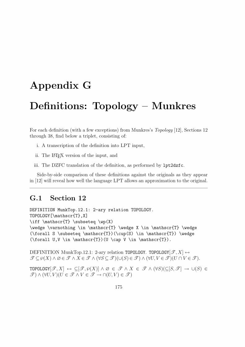
Appendix G
Definitions: Topology – Munkres
For each definition (with a few exceptions) from Munkres’s Topology [12], Sections 12through 38, find below a triplet, consisting of:
i. A transcription of the definition into LPT input,
ii. The LATEX version of the input, and
iii. The DZFC translation of the definition, as performed by lpt2dzfc.
Side-by-side comparison of these definitions against the originals as they appearin [12] will reveal how well the language LPT allows an approximation to the original.
G.1 Section 12
DEFINITION MunkTop.12.1: 2-ary relation TOPOLOGY.
TOPOLOGY[\mathscrT,X]
\iff \mathscrT \subseteq \wp(X)
\wedge \varnothing \in \mathscrT \wedge X \in \mathscrT \wedge
(\forall S \subseteq \mathscrT)(\cup(S) \in \mathscrT) \wedge
(\forall U,V \in \mathscrT)(U \cap V \in \mathscrT).
DEFINITION MunkTop.12.1: 2-ary relation TOPOLOGY. TOPOLOGY[T , X] ↔T ⊆℘(X) ∧∅∈T ∧X ∈T ∧ (∀S⊆T )(∪(S)∈T ) ∧ (∀U, V ∈T )(U ∩ V ∈T ).
TOPOLOGY[T , X] ↔ ⊆[T , ℘(X)] ∧ ∅ ∈ T ∧ X ∈ T ∧ (∀S)(⊆[S, T ] → ∪(S) ∈T ) ∧ (∀U, V )(U ∈ T ∧ V ∈ T → ∩(U, V ) ∈ T )
175
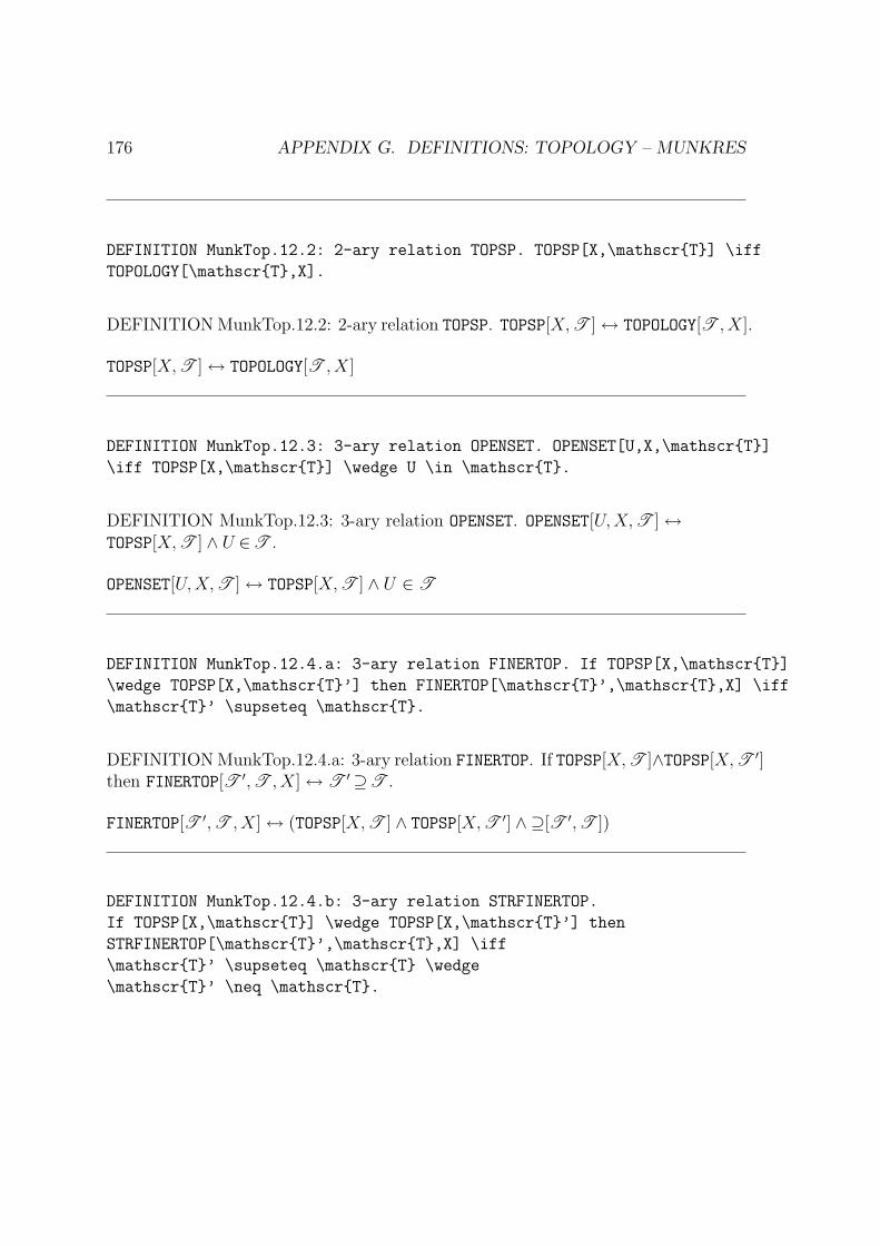
176 APPENDIX G. DEFINITIONS: TOPOLOGY – MUNKRES
DEFINITION MunkTop.12.2: 2-ary relation TOPSP. TOPSP[X,\mathscrT] \iff
TOPOLOGY[\mathscrT,X].
DEFINITION MunkTop.12.2: 2-ary relation TOPSP. TOPSP[X, T ] ↔ TOPOLOGY[T , X].
TOPSP[X, T ] ↔ TOPOLOGY[T , X]
DEFINITION MunkTop.12.3: 3-ary relation OPENSET. OPENSET[U,X,\mathscrT]
\iff TOPSP[X,\mathscrT] \wedge U \in \mathscrT.
DEFINITION MunkTop.12.3: 3-ary relation OPENSET. OPENSET[U,X, T ] ↔TOPSP[X, T ] ∧ U ∈T .
OPENSET[U,X, T ] ↔ TOPSP[X, T ] ∧ U ∈ T
DEFINITION MunkTop.12.4.a: 3-ary relation FINERTOP. If TOPSP[X,\mathscrT]
\wedge TOPSP[X,\mathscrT’] then FINERTOP[\mathscrT’,\mathscrT,X] \iff
\mathscrT’ \supseteq \mathscrT.
DEFINITION MunkTop.12.4.a: 3-ary relation FINERTOP. If TOPSP[X, T ]∧TOPSP[X, T ′]then FINERTOP[T ′,T , X] ↔ T ′⊇T .
FINERTOP[T ′,T , X] ↔ (TOPSP[X, T ] ∧ TOPSP[X, T ′] ∧ ⊇[T ′,T ])
DEFINITION MunkTop.12.4.b: 3-ary relation STRFINERTOP.
If TOPSP[X,\mathscrT] \wedge TOPSP[X,\mathscrT’] then
STRFINERTOP[\mathscrT’,\mathscrT,X] \iff
\mathscrT’ \supseteq \mathscrT \wedge
\mathscrT’ \neq \mathscrT.

G.2. SECTION 13 177
DEFINITION MunkTop.12.4.b: 3-ary relation STRFINERTOP. If TOPSP[X, T ]∧TOPSP[X, T ′] then STRFINERTOP[T ′, T , X] ↔ T ′⊇T ∧T ′ 6= T .
STRFINERTOP[T ′,T , X] ↔ (TOPSP[X, T ] ∧ TOPSP[X, T ′] ∧ ⊇[T ′, T ] ∧ ¬(T ′ = T ))
DEFINITION MunkTop.12.4.c: 3-ary relation COARSERTOP.
If TOPSP[X,\mathscrT] \wedge TOPSP[X,\mathscrT’] then
COARSERTOP[\mathscrT’,\mathscrT,X] \iff
\mathscrT’ \subseteq \mathscrT.
DEFINITION MunkTop.12.4.c: 3-ary relation COARSERTOP. If TOPSP[X, T ]∧TOPSP[X, T ′]then COARSERTOP[T ′,T , X] ↔ T ′⊆T .
COARSERTOP[T ′,T , X] ↔ (TOPSP[X, T ] ∧ TOPSP[X, T ′] ∧ ⊆[T ′,T ])
DEFINITION MunkTop.12.4.d: 3-ary relation STRCOARSERTOP.
If TOPSP[X,\mathscrT] \wedge TOPSP[X,\mathscrT’] then
STRCOARSERTOP[\mathscrT’,\mathscrT,X] \iff
\mathscrT’ \subseteq \mathscrT \wedge \mathscrT’ \neq \mathscrT.
DEFINITION MunkTop.12.4.d: 3-ary relation STRCOARSERTOP. If TOPSP[X, T ] ∧TOPSP[X, T ′] then STRCOARSERTOP[T ′,T , X] ↔ T ′⊆T ∧T ′ 6= T .
STRCOARSERTOP[T ′,T , X] ↔ (TOPSP[X, T ]∧TOPSP[X, T ′]∧⊆[T ′, T ]∧¬(T ′ = T ))
G.2 Section 13
DEFINITION MunkTop.13.1: 2-ary relation TOPBASIS. TOPBASIS[\mathscrB,X]
\iff \mathscrB \subseteq \wp(X) \wedge
(\forall x \in X)(\exists B \in \mathscrB)(x \in B) \wedge
(\forall x \in X)(\forall B_1, B_2 \in \mathscrB)
(\exists B_3 \in \mathscrB)(
x \in B_3 \wedge B_3 \subseteq B_1 \cap B_2
).

178 APPENDIX G. DEFINITIONS: TOPOLOGY – MUNKRES
DEFINITION MunkTop.13.1: 2-ary relation TOPBASIS. TOPBASIS[B, X] ↔ B⊆℘(X)∧(∀x∈X)(∃B ∈B)(x∈B)∧ (∀x∈X)(∀B1, B2 ∈B)(∃B3 ∈B)(x∈B3∧B3⊆B1∩B2).
TOPBASIS[B, X] ↔ ⊆[B, ℘(X)] ∧ (∀x)(x ∈ X → (∃B)(B ∈ B ∧ x ∈ B)) ∧ (∀x)(x ∈X → (∀B1, B2)(B1 ∈ B ∧B2 ∈ B → (∃B3)(B3 ∈ B ∧ x ∈ B3 ∧ ⊆[B3,∩(B1, B2)])))
DEFINITION MunkTop.13.2: 2-ary function Basisgentop.
If TOPBASIS[\mathscrB,X] then
Basisgentop(\mathscrB,X) \simeq (!\mathscrT \subseteq \wp(X))(
(\forall U \subseteq X)(U \in \mathscrT \iff
(\forall x \in U)(\exists B \in \mathscrB)(
x \in B \wedge B \subseteq U
)
)
).
DEFINITION MunkTop.13.2: 2-ary function Basisgentop. If TOPBASIS[B, X] thenBasisgentop(B, X) ' (!T ⊆℘(X))((∀U ⊆X)(U ∈T ↔ (∀x∈U)(∃B ∈B)(x∈B ∧B⊆U))).
Basisgentop(B, X) ' (ιy0)(TOPBASIS[B, X]∧y0 ' (ιx0)(∃T )(x0 = T ∧((∀U)(⊆[U,X]→ U ∈ T ↔ (∀x)(x ∈ U → (∃B)(B ∈ B ∧ x ∈ B ∧ ⊆[B, U ])))) ∧ (⊆[T , ℘(X)])))
DEFINITION MunkTop.13.3.a.basis: 0-ary function Stdrealtopbasis.
Stdrealtopbasis \simeq U \subseteq \mathbbR :
(\exists a,b \in \mathbbR)(
U = x \in \mathbbR : a <_R x <_R b
)
.
DEFINITION MunkTop.13.3.a.basis: 0-ary function Stdrealtopbasis.Stdrealtopbasis ' U ⊆R : (∃a, b∈R)(U = x∈R : a<R x<R b).Stdrealtopbasis ' (ιx1)(∀z0)(z0 ∈ x1 ↔ (∃U)(z0 = U∧((∃a, b)(a ∈ R∧b ∈ R∧U =(ιy0)(∀x0)(x0 ∈ y0 ↔ (∃x)(x0 = x ∧ (<R[a, x] ∧<R[x, b]) ∧ (x ∈ R))))) ∧ (⊆[U,R])))

G.2. SECTION 13 179
DEFINITION MunkTop.13.3.a: 0-ary function Stdrealtop. Stdrealtop \simeq
Basisgentop(Stdrealtopbasis,\mathbbR).
DEFINITION MunkTop.13.3.a: 0-ary function Stdrealtop. Stdrealtop 'Basisgentop(Stdrealtopbasis,R).
Stdrealtop ' Basisgentop(Stdrealtopbasis,R)
DEFINITION MunkTop.13.3.b: 0-ary function Lowerlimitrealtop.
Lowerlimitrealtop \simeq Basisgentop(
U \subseteq \mathbbR :
(\exists a,b \in \mathbbR)(
U = x \in \mathbbR : a \leq_R x <_R b
)
,
\mathbbR
).
DEFINITION MunkTop.13.3.b: 0-ary function Lowerlimitrealtop.Lowerlimitrealtop ' Basisgentop(U ⊆R : (∃a, b∈R)(U = x∈R : a≤R x<R b),R).
Lowerlimitrealtop ' Basisgentop((ιx1)(∀z0)(z0 ∈ x1 ↔ (∃U)(z0 = U∧((∃a, b)(a ∈R∧b ∈ R∧U = (ιy0)(∀x0)(x0 ∈ y0 ↔ (∃x)(x0 = x ∧ (≤R[a, x] ∧ <R[x, b]) ∧ (x ∈R))))) ∧ (⊆[U,R]))),R)
DEFINITION MunkTop.13.3.c: 0-ary function Krealtop. Krealtop \simeq
Basisgentop(
Stdrealtopbasis \cup
V \subseteq \mathbbR :
(\exists W \in Stdrealtopbasis)(
V = W \less Incl_FrR(1_N/n) : n \in \mathbbN
)
,
\mathbbR
).

180 APPENDIX G. DEFINITIONS: TOPOLOGY – MUNKRES
DEFINITION MunkTop.13.3.c: 0-ary function Krealtop. Krealtop 'Basisgentop(Stdrealtopbasis∪V ⊆R : (∃W ∈ Stdrealtopbasis)(V = W\InclFrR(1N /n) : n∈N),R).
Krealtop ' Basisgentop(∪(Stdrealtopbasis, (ιx1)(∀z0)(z0 ∈ x1 ↔ (∃V )(z0 =V ∧ ((∃W )(W ∈ Stdrealtopbasis∧V = \(W, (ιy0)(∀x0)(x0 ∈ y0 ↔ (∃n)(x0 =InclFrR(/(1N, n)) ∧ (n ∈ N)))))) ∧ (⊆[V,R])))),R)
DEFINITION MunkTop.13.4.a: 2-ary relation TOPSUBBASIS.
TOPSUBBASIS[\mathscrS,X]
\iff \mathscrS \subseteq \wp(X) \wedge \cup(\mathscrS) = X.
DEFINITION MunkTop.13.4.a: 2-ary relation TOPSUBBASIS. TOPSUBBASIS[S , X] ↔S ⊆℘(X) ∧ ∪(S ) = X.
TOPSUBBASIS[S , X] ↔ ⊆[S , ℘(X)] ∧ ∪(S ) = X
DEFINITION MunkTop.13.4.b: 2-ary function Subbasisgentop.
Subbasisgentop(\mathscrS,X) \simeq U \subseteq X :
(\exists \mathscrA \subseteq \wp(\mathscrS))(
(\forall A \in \mathscrA)(DFIN[A]) \wedge
U = \cup(\cap(S) : S \in A)
)
.
DEFINITION MunkTop.13.4.b: 2-ary function Subbasisgentop.Subbasisgentop(S , X) ' U ⊆X : (∃A ⊆℘(S ))((∀A∈A )(DFIN[A])∧U = ∪(∩(S) :S ∈A)).
Subbasisgentop(S , X) ' (ιx1)(∀z0)(z0 ∈ x1 ↔ (∃U)(z0 = U∧((∃A )(⊆[A , ℘(S )]∧(∀A)(A ∈ A → DFIN[A]) ∧ U = ∪((ιy0)(∀x0)(x0 ∈ y0 ↔ (∃S)(x0 = ∩(S) ∧ (S ∈A)))))) ∧ (⊆[U,X])))

G.3. SECTION 14 181
G.3 Section 14
DEFINITION MunkTop.14.1: 4-ary function Oointerval. If SSORD[R,X]
\wedge a,b \in X then Oointerval(a,b,X,R) \simeq
x \in X : a \infixrlR x \infixrlR b.
DEFINITION MunkTop.14.1: 4-ary function Oointerval. If SSORD[R,X] ∧ a, b∈Xthen Oointerval(a, b, X, R) ' x∈X : aRxRb.
Oointerval(a, b, X, R) ' (ιz0)(SSORD[R, X] ∧ a ∈ X ∧ b ∈ X ∧ z0 ' (ιy0)(∀x0)(x0 ∈y0 ↔ (∃x)(x0 = x ∧ ($0(a, x) ∈ R ∧$0(x, b) ∈ R) ∧ (x ∈ X))))
DEFINITION MunkTop.14.1.A: 3-ary relation OOINTERVAL. If SSORD[R,X]
\wedge U \subseteq X then OOINTERVAL[U,X,R] \iff
(\exists a,b \in X)(U = Oointerval(a,b,X,R)).
DEFINITION MunkTop.14.1.A: 3-ary relation OOINTERVAL. If SSORD[R,X] ∧ U ⊆Xthen OOINTERVAL[U,X, R] ↔ (∃a, b∈X)(U = Oointerval(a, b, X, R)).
OOINTERVAL[U,X, R] ↔ (SSORD[R,X] ∧ ⊆[U,X] ∧ (∃a, b)(a ∈ X ∧ b ∈ X ∧ U =Oointerval(a, b, X, R)))
DEFINITION MunkTop.14.2: 4-ary function Ocinterval. If SSORD[R,X]
\wedge a,b \in X then Ocinterval(a,b,X,R) \simeq
x \in X : a \infixrlR x \infixrlR b \vee x = b.
DEFINITION MunkTop.14.2: 4-ary function Ocinterval. If SSORD[R,X] ∧ a, b∈Xthen Ocinterval(a, b, X, R) ' x∈X : aRxRb ∨ x = b.
Ocinterval(a, b, X, R) ' (ιz0)(SSORD[R, X] ∧ a ∈ X ∧ b ∈ X ∧ z0 ' (ιy0)(∀x0)(x0 ∈y0 ↔ (∃x)(x0 = x ∧ ($0(a, x) ∈ R ∧$0(x, b) ∈ R ∨ x = b) ∧ (x ∈ X))))
DEFINITION MunkTop.14.2.A: 3-ary relation OCINTERVAL. If SSORD[R,X]
\wedge W \subseteq X then OCINTERVAL[W,X,R] \iff
(\exists a,b \in X)(W = Ocinterval(a,b,X,R)).

182 APPENDIX G. DEFINITIONS: TOPOLOGY – MUNKRES
DEFINITION MunkTop.14.2.A: 3-ary relation OCINTERVAL. If SSORD[R,X]∧W ⊆Xthen OCINTERVAL[W,X, R] ↔ (∃a, b∈X)(W = Ocinterval(a, b, X,R)).
OCINTERVAL[W,X, R] ↔ (SSORD[R, X] ∧ ⊆[W,X] ∧ (∃a, b)(a ∈ X ∧ b ∈ X ∧ W =Ocinterval(a, b, X, R)))
DEFINITION MunkTop.14.3: 4-ary function Cointerval. If SSORD[R,X]
\wedge a,b \in X then Cointerval(a,b,X,R) \simeq
x \in X : a \infixrlR x \infixrlR b \vee x = a.
DEFINITION MunkTop.14.3: 4-ary function Cointerval. If SSORD[R,X] ∧ a, b∈Xthen Cointerval(a, b, X, R) ' x∈X : aRxRb ∨ x = a.Cointerval(a, b, X, R) ' (ιz0)(SSORD[R, X] ∧ a ∈ X ∧ b ∈ X ∧ z0 ' (ιy0)(∀x0)(x0 ∈y0 ↔ (∃x)(x0 = x ∧ ($0(a, x) ∈ R ∧$0(x, b) ∈ R ∨ x = a) ∧ (x ∈ X))))
DEFINITION MunkTop.14.3.A: 3-ary relation COINTERVAL. If SSORD[R,X]
\wedge W \subseteq X then COINTERVAL[W,X,R] \iff
(\exists a,b \in X)(W = Cointerval(a,b,X,R)).
DEFINITION MunkTop.14.3.A: 3-ary relation COINTERVAL. If SSORD[R,X]∧W ⊆Xthen COINTERVAL[W,X, R] ↔ (∃a, b∈X)(W = Cointerval(a, b, X,R)).
COINTERVAL[W,X, R] ↔ (SSORD[R, X] ∧ ⊆[W,X] ∧ (∃a, b)(a ∈ X ∧ b ∈ X ∧ W =Cointerval(a, b, X, R)))
DEFINITION MunkTop.14.4: 4-ary function Ccinterval. If SSORD[R,X]
\wedge a,b \in X then Ccinterval(a,b,X,R) \simeq
x \in X : a \infixrlR x \infixrlR b \vee x = a \vee x = b.
DEFINITION MunkTop.14.4: 4-ary function Ccinterval. If SSORD[R,X] ∧ a, b∈Xthen Ccinterval(a, b, X, R) ' x∈X : aRxRb ∨ x = a ∨ x = b.Ccinterval(a, b, X, R) ' (ιz0)(SSORD[R, X] ∧ a ∈ X ∧ b ∈ X ∧ z0 ' (ιy0)(∀x0)(x0 ∈y0 ↔ (∃x)(x0 = x ∧ ($0(a, x) ∈ R ∧$0(x, b) ∈ R ∨ x = a ∨ x = b) ∧ (x ∈ X))))
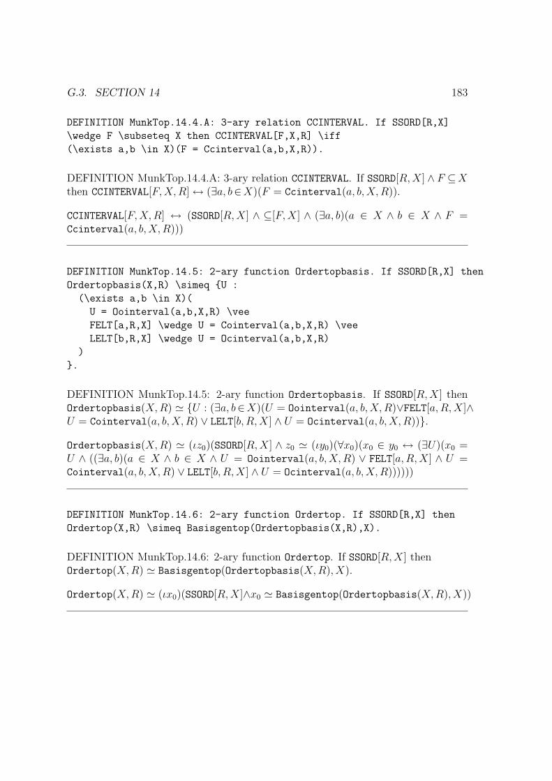
G.3. SECTION 14 183
DEFINITION MunkTop.14.4.A: 3-ary relation CCINTERVAL. If SSORD[R,X]
\wedge F \subseteq X then CCINTERVAL[F,X,R] \iff
(\exists a,b \in X)(F = Ccinterval(a,b,X,R)).
DEFINITION MunkTop.14.4.A: 3-ary relation CCINTERVAL. If SSORD[R, X] ∧ F ⊆Xthen CCINTERVAL[F,X,R] ↔ (∃a, b∈X)(F = Ccinterval(a, b, X, R)).
CCINTERVAL[F, X, R] ↔ (SSORD[R, X] ∧ ⊆[F,X] ∧ (∃a, b)(a ∈ X ∧ b ∈ X ∧ F =Ccinterval(a, b, X, R)))
DEFINITION MunkTop.14.5: 2-ary function Ordertopbasis. If SSORD[R,X] then
Ordertopbasis(X,R) \simeq U :
(\exists a,b \in X)(
U = Oointerval(a,b,X,R) \vee
FELT[a,R,X] \wedge U = Cointerval(a,b,X,R) \vee
LELT[b,R,X] \wedge U = Ocinterval(a,b,X,R)
)
.
DEFINITION MunkTop.14.5: 2-ary function Ordertopbasis. If SSORD[R, X] thenOrdertopbasis(X, R) ' U : (∃a, b∈X)(U = Oointerval(a, b,X,R)∨FELT[a,R, X]∧U = Cointerval(a, b, X, R) ∨ LELT[b, R, X] ∧ U = Ocinterval(a, b, X, R)).
Ordertopbasis(X, R) ' (ιz0)(SSORD[R, X] ∧ z0 ' (ιy0)(∀x0)(x0 ∈ y0 ↔ (∃U)(x0 =U ∧ ((∃a, b)(a ∈ X ∧ b ∈ X ∧ U = Oointerval(a, b, X, R) ∨ FELT[a,R, X] ∧ U =Cointerval(a, b, X, R) ∨ LELT[b, R, X] ∧ U = Ocinterval(a, b, X, R))))))
DEFINITION MunkTop.14.6: 2-ary function Ordertop. If SSORD[R,X] then
Ordertop(X,R) \simeq Basisgentop(Ordertopbasis(X,R),X).
DEFINITION MunkTop.14.6: 2-ary function Ordertop. If SSORD[R, X] thenOrdertop(X, R) ' Basisgentop(Ordertopbasis(X,R), X).
Ordertop(X, R) ' (ιx0)(SSORD[R, X]∧x0 ' Basisgentop(Ordertopbasis(X, R), X))
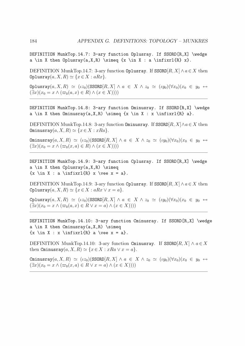
184 APPENDIX G. DEFINITIONS: TOPOLOGY – MUNKRES
DEFINITION MunkTop.14.7: 3-ary function Oplusray. If SSORD[R,X] \wedge
a \in X then Oplusray(a,X,R) \simeq x \in X : a \infixrlR x.
DEFINITION MunkTop.14.7: 3-ary function Oplusray. If SSORD[R,X]∧ a∈X thenOplusray(a,X,R) ' x∈X : aRx.Oplusray(a,X,R) ' (ιz0)(SSORD[R,X] ∧ a ∈ X ∧ z0 ' (ιy0)(∀x0)(x0 ∈ y0 ↔(∃x)(x0 = x ∧ ($0(a, x) ∈ R) ∧ (x ∈ X))))
DEFINITION MunkTop.14.8: 3-ary function Ominusray. If SSORD[R,X] \wedge
a \in X then Ominusray(a,X,R) \simeq x \in X : x \infixrlR a.
DEFINITION MunkTop.14.8: 3-ary function Ominusray. If SSORD[R, X]∧a∈X thenOminusray(a,X,R) ' x∈X : xRa.Ominusray(a,X,R) ' (ιz0)(SSORD[R,X] ∧ a ∈ X ∧ z0 ' (ιy0)(∀x0)(x0 ∈ y0 ↔(∃x)(x0 = x ∧ ($0(x, a) ∈ R) ∧ (x ∈ X))))
DEFINITION MunkTop.14.9: 3-ary function Cplusray. If SSORD[R,X] \wedge
a \in X then Cplusray(a,X,R) \simeq
x \in X : a \infixrlR x \vee x = a.
DEFINITION MunkTop.14.9: 3-ary function Cplusray. If SSORD[R,X]∧ a∈X thenCplusray(a,X,R) ' x∈X : aRx ∨ x = a.Cplusray(a,X,R) ' (ιz0)(SSORD[R,X] ∧ a ∈ X ∧ z0 ' (ιy0)(∀x0)(x0 ∈ y0 ↔(∃x)(x0 = x ∧ ($0(a, x) ∈ R ∨ x = a) ∧ (x ∈ X))))
DEFINITION MunkTop.14.10: 3-ary function Cminusray. If SSORD[R,X] \wedge
a \in X then Cminusray(a,X,R) \simeq
x \in X : x \infixrlR a \vee x = a.
DEFINITION MunkTop.14.10: 3-ary function Cminusray. If SSORD[R, X] ∧ a∈Xthen Cminusray(a,X, R) ' x∈X : xRa ∨ x = a.Cminusray(a,X,R) ' (ιz0)(SSORD[R,X] ∧ a ∈ X ∧ z0 ' (ιy0)(∀x0)(x0 ∈ y0 ↔(∃x)(x0 = x ∧ ($0(x, a) ∈ R ∨ x = a) ∧ (x ∈ X))))

G.4. SECTION 15 185
G.4 Section 15
DEFINITION MunkTop.15.1: 4-ary function Prodtopbasis.
If TOPSP[X,\mathscrT] \wedge
TOPSP[Y,\mathscrT’] then Prodtopbasis(X,\mathscrT,Y,\mathscrT’)
\simeq U \times V : U \in \mathscrT \wedge V \in \mathscrT’.
DEFINITION MunkTop.15.1: 4-ary function Prodtopbasis. If TOPSP[X, T ]∧TOPSP[Y, T ′] then Prodtopbasis(X, T , Y, T ′) ' U × V : U ∈T ∧ V ∈T ′.Prodtopbasis(X, T , Y, T ′) ' (ιz0)(TOPSP[X, T ]∧TOPSP[Y, T ′]∧z0 ' (ιy0)(∀x0)(x0 ∈y0 ↔ (∃U, V )(x0 = ×(U, V ) ∧ (U ∈ T ∧ V ∈ T ′))))
DEFINITION MunkTop.15.2: 4-ary function Prodtop. If TOPSP[X,\mathscrT]
\wedge TOPSP[Y,\mathscrT’] then Prodtop(X,\mathscrT,Y,\mathscrT’)
\simeq Basisgentop(Prodtopbasis(X,\mathscrT,Y,\mathscrT’),X).
DEFINITION MunkTop.15.2: 4-ary function Prodtop. If TOPSP[X, T ]∧TOPSP[Y, T ′]then Prodtop(X, T , Y, T ′) ' Basisgentop(Prodtopbasis(X, T , Y, T ′), X).
Prodtop(X, T , Y, T ′) ' (ιx0)(TOPSP[X, T ] ∧ TOPSP[Y, T ′] ∧ x0 'Basisgentop(Prodtopbasis(X, T , Y, T ′), X))
DEFINITION MunkTop.15.3: 2-ary function \pi_1. \pi_1(x,y) \simeq x.
DEFINITION MunkTop.15.3: 2-ary function π1. π1(x, y) ' x.
π1(x, y) ' x
DEFINITION MunkTop.15.4: 2-ary function \pi_2. \pi_2(x,y) \simeq y.
DEFINITION MunkTop.15.4: 2-ary function π2. π2(x, y) ' y.
π2(x, y) ' y
186 APPENDIX G. DEFINITIONS: TOPOLOGY – MUNKRES
DEFINITION MunkTop.15.5: 1-ary function \pi_1. If (\exists u,v)
(x = <u,v>) then \pi_1(x) \simeq u. Otherwise \pi_1(x) \up.
DEFINITION MunkTop.15.5: 1-ary function π1. If (∃u, v)(x = 〈u, v〉) then π1(x) 'u. Otherwise π1(x)↑.
π1(x) ' (ιx0)(((∃u, v)x = $0(u, v) ∧ x0 ' u))
DEFINITION MunkTop.15.6: 1-ary function \pi_2. If (\exists u,v)
(x = <u,v>) then \pi_2(x) \simeq v. Otherwise \pi_2(x) \up.
DEFINITION MunkTop.15.6: 1-ary function π2. If (∃u, v)(x = 〈u, v〉) then π2(x) 'v. Otherwise π2(x)↑.
π2(x) ' (ιx0)(((∃u, v)x = $0(u, v) ∧ x0 ' v))
G.5 Section 16
DEFINITION MunkTop.16.1: 3-ary function Subspacetop.
If TOPSP[X,\mathscrT] \wedge Y \subseteq X then
Subspacetop(Y,X,\mathscrT) \simeq Y \cap U : U \in \mathscrT.
DEFINITION MunkTop.16.1: 3-ary function Subspacetop. If TOPSP[X, T ]∧ Y ⊆Xthen Subspacetop(Y, X, T ) ' Y ∩ U : U ∈T .
Subspacetop(Y, X, T ) ' (ιz0)(TOPSP[X, T ] ∧ ⊆[Y,X] ∧ z0 ' (ιy0)(∀x0)(x0 ∈ y0 ↔(∃Y, U)(x0 = ∩(Y, U) ∧ (U ∈ T ))))
DEFINITION MunkTop.16.2: 4-ary relation SUBSPACE.
If TOPSP[X,\mathscrT] \wedge Y \subseteq X then
SUBSPACE[Y,\mathscrT’,X,\mathscrT] \iff
\mathscrT’ = Subspacetop(Y,X,\mathscrT).

G.5. SECTION 16 187
DEFINITION MunkTop.16.2: 4-ary relation SUBSPACE. If TOPSP[X, T ]∧Y ⊆X thenSUBSPACE[Y, T ′, X, T ] ↔ T ′ = Subspacetop(Y, X, T ).
SUBSPACE[Y, T ′, X, T ] ↔ (TOPSP[X, T ] ∧ ⊆[Y,X] ∧T ′ = Subspacetop(Y,X, T ))
DEFINITION MunkTop.16.3: 4-ary function Dictionaryorder. If SSORD[R,A]
\wedge SSORD[S,B] then Dictionaryorder(R,A,S,B) \simeq (!T)(
(\forall y)(
y \in T \iff (\exists p,q,r,s)(
y = <<p,q>,<r,s>> \wedge p,r \in A \wedge q,s \in B \wedge
( p \infixrlR r \vee p = r \wedge q \infixrlS s )
)
)
).
DEFINITION MunkTop.16.3: 4-ary function Dictionaryorder. If SSORD[R, A] ∧SSORD[S, B] then Dictionaryorder(R, A, S, B) ' (!T )((∀y)(y ∈T ↔ (∃p, q, r, s)(y =〈〈p, q〉 , 〈r, s〉〉 ∧ p, r∈A ∧ q, s∈B ∧ (pRr ∨ p = r ∧ qSs)))).
Dictionaryorder(R, A, S, B) ' (ιy0)(SSORD[R, A]∧SSORD[S, B]∧y0 ' (ιx0)(∃T )(x0 =T ∧ ((∀y)y ∈ T ↔ (∃p, q, r, s)y = $0($0(p, q), $0(r, s))∧ p ∈ A∧ r ∈ A∧ q ∈ B ∧ s ∈B ∧$0(p, r) ∈ R ∨ p = r ∧$0(q, s) ∈ S)))
DEFINITION MunkTop.16.4: 0-ary function Orderedsquare.
If I = Ccinterval(0_R,1_R,\mathbbR,<x,y> : x <_R y) \wedge
R = Dictionaryorder(<x,y> : x <_R y,I,<x,y> : x <_R y,I) then
Orderedsquare \simeq <I \times I, Ordertop(I \times I,R)>.
DEFINITION MunkTop.16.4: 0-ary function Orderedsquare.If I = Ccinterval(0R, 1R,R, 〈x, y〉 : x<R y) ∧ R = Dictionaryorder(〈x, y〉 :
x<R y, I, 〈x, y〉 : x<R y, I) then Orderedsquare ' 〈I × I, Ordertop(I × I, R)〉.Orderedsquare ' (ιz0)(I = Ccinterval(0R, 1R,R, (ιy0)(∀x0)(x0 ∈ y0 ↔ (∃x, y)(x0 =$0(x, y) ∧ (<R[x, y])))) ∧ R = Dictionaryorder((ιy0)(∀x0)(x0 ∈ y0 ↔ (∃x, y)(x0 =$0(x, y)∧(<R[x, y]))), I, (ιy0)(∀x0)(x0 ∈ y0 ↔ (∃x, y)(x0 = $0(x, y)∧(<R[x, y]))), I)∧z0 ' $0(×(I, I), Ordertop(×(I, I), R)))

188 APPENDIX G. DEFINITIONS: TOPOLOGY – MUNKRES
DEFINITION MunkTop.16.5: 3-ary relation CONVEX. If SSORD[R,X]
\wedge Y \subseteq X then CONVEX[Y,X,R] \iff
(\forall a,b \in Y)(
Oointerval(a,b,X,R) \subseteq Y
).
DEFINITION MunkTop.16.5: 3-ary relation CONVEX. If SSORD[R, X] ∧ Y ⊆X thenCONVEX[Y, X, R] ↔ (∀a, b∈Y )(Oointerval(a, b, X, R)⊆Y ).
CONVEX[Y, X, R] ↔ (SSORD[R,X] ∧ ⊆[Y,X] ∧ (∀a, b)(a ∈ Y ∧ b ∈ Y →⊆[Oointerval(a, b, X, R), Y ]))
G.6 Section 17
DEFINITION MunkTop.17.1: 3-ary relation CLOSEDSET. If A \subseteq X then
CLOSEDSET[A,X,\mathscrT] \iff TOPSP[X,\mathscrT] \wedge
OPENSET[X \less A,X,\mathscrT].
DEFINITION MunkTop.17.1: 3-ary relation CLOSEDSET. If A⊆X thenCLOSEDSET[A,X, T ] ↔ TOPSP[X, T ] ∧ OPENSET[X\A,X, T ].
CLOSEDSET[A,X, T ] ↔ (⊆[A,X] ∧ TOPSP[X, T ] ∧ OPENSET[\(X, A), X, T ])
DEFINITION MunkTop.17.2: 1-ary function Interior.
If TOPSP[X,\mathscrT] \wedge A \subseteq X then Interior(A) \simeq
\cup(U \in \mathscrT : U \subseteq A).
DEFINITION MunkTop.17.2: 1-ary function Interior. If TOPSP[X, T ]∧A⊆X thenInterior(A) ' ∪(U ∈T : U ⊆A).
Interior(A) ' (ιz0)(TOPSP[X, T ]∧⊆[A,X]∧z0 ' ∪((ιy0)(∀x0)(x0 ∈ y0 ↔ (∃U)(x0 =U ∧ (⊆[U,A]) ∧ (U ∈ T )))))
G.6. SECTION 17 189
DEFINITION MunkTop.17.3: 3-ary function Closure. If
TOPSP[X,\mathscrT] \wedge A \subseteq X then Closure(A,X,T) \simeq
\cap(F : A \subseteq F \wedge CLOSEDSET[F,X,\mathscrT]).
DEFINITION MunkTop.17.3: 3-ary function Closure. If TOPSP[X, T ]∧A⊆X thenClosure(A,X, T ) ' ∩(F : A⊆F ∧ CLOSEDSET[F, X, T ]).Closure(A,X, T ) ' (ιz0)(TOPSP[X, T ] ∧ ⊆[A,X] ∧ z0 ' ∩((ιy0)(∀x0)(x0 ∈ y0 ↔(∃F )(x0 = F ∧ (⊆[A,F ] ∧ CLOSEDSET[F, X, T ])))))
DEFINITION MunkTop.17.4: 2-ary relation INTERSECTS. INTERSECTS[A,B] \iff
A \cap B \neq \varnothing.
DEFINITION MunkTop.17.4: 2-ary relation INTERSECTS. INTERSECTS[A,B] ↔ A ∩B 6= ∅.
INTERSECTS[A,B] ↔ ¬(∩(A,B) = ∅)
DEFINITION MunkTop.17.4.5: 2-ary relation DISJOINT. DISJOINT[A,B] \iff
A \cap B = \varnothing.
DEFINITION MunkTop.17.4.5: 2-ary relation DISJOINT. DISJOINT[A,B] ↔ A∩B =∅.
DISJOINT[A,B] ↔ ∩(A,B) = ∅
DEFINITION MunkTop.17.5: 4-ary relation NBHD. If TOPSP[X,\mathscrT]
\wedge x \in X \wedge U \in \mathscrT then
NBHD[U,x,X,\mathscrT] \iff x \in U.
DEFINITION MunkTop.17.5: 4-ary relation NBHD. If TOPSP[X, T ] ∧ x∈X ∧ U ∈Tthen NBHD[U, x,X, T ] ↔ x∈U .
NBHD[U, x, X, T ] ↔ (TOPSP[X, T ] ∧ x ∈ X ∧ U ∈ T ∧ x ∈ U)

190 APPENDIX G. DEFINITIONS: TOPOLOGY – MUNKRES
DEFINITION MunkTop.17.6: 4-ary relation LIMITPT.
If TOPSP[X,\mathscrT] \wedge x \in X \wedge A \subseteq X then
LIMITPT[x,A,X,\mathscrT] \iff (\forall U)(
NBHD[U,x,X,\mathscrT] \implies INTERSECTS[U,A \less x]
).
DEFINITION MunkTop.17.6: 4-ary relation LIMITPT. If TOPSP[X, T ]∧x∈X∧A⊆Xthen LIMITPT[x,A, X, T ] ↔ (∀U)(NBHD[U, x,X, T ] → INTERSECTS[U,A\x]).
LIMITPT[x,A, X, T ] ↔ (TOPSP[X, T ] ∧ x ∈ X ∧ ⊆[A,X] ∧ (∀U) NBHD[U, x, X, T ] →INTERSECTS[U, \(A, (ιx0)(∀y0)(y0 ∈ x0 ↔ y0 = x))])
DEFINITION MunkTop.17.7: 3-ary relation TOPCONV.
If TOPSP[X,\mathscrT] \wedge f \in Maps(\mathbbN,X) \wedge
x \in X then TOPCONV[f,x,\mathscrT] \iff
(\forall U \in \mathscrT)(
NBHD[U,x,X,\mathscrT] \implies
(\exists N \in \mathbbN)(\forall n >_N N)(f(n) \in U)
).
DEFINITION MunkTop.17.7: 3-ary relation TOPCONV. If TOPSP[X, T ]∧f ∈ Maps(N, X)∧x∈X then TOPCONV[f, x, T ] ↔ (∀U ∈T )(NBHD[U, x,X, T ] →(∃N ∈N)(∀n>N N)(f(n)∈U)).
TOPCONV[f, x, T ] ↔ (TOPSP[X, T ] ∧ f ∈ Maps(N, X) ∧ x ∈ X ∧ (∀U)(U ∈ T →NBHD[U, x, X, T ] → (∃N)(N ∈ N∧(∀n)(>N[n,N ] → (ιx0)($0(n, x0) ∈ f) ∈ U))))
DEFINITION MunkTop.17.8: 2-ary relation HAUSDORFF.
If TOPSP[X,\mathscrT] then HAUSDORFF[X,\mathscrT] \iff
(\forall x,y \in X)(
x \neq y \implies
(\exists U,V \in \mathscrT)(
x \in U \wedge y \in V \wedge DISJOINT[U,V]
)
).

G.7. SECTION 18 191
DEFINITION MunkTop.17.8: 2-ary relation HAUSDORFF. If TOPSP[X, T ] then
HAUSDORFF[X, T ] ↔ (∀x, y ∈X)(x 6= y → (∃U, V ∈T )(x∈U∧y ∈V ∧DISJOINT[U, V ])).
HAUSDORFF[X, T ] ↔ (TOPSP[X, T ] ∧ (∀x, y)(x ∈ X ∧ y ∈ X → ¬(x = y) →(∃U, V )(U ∈ T ∧ V ∈ T ∧ x ∈ U ∧ y ∈ V ∧ DISJOINT[U, V ])))
DEFINITION MunkTop.17.9: 3-ary relation TOPLIMIT.
If HAUSDORFF[X,\mathscrT] \wedge
(\exists y)(TOPCONV[f,y,\mathscrT]) then
TOPLIMIT[x,f,\mathscrT] \iff
x = (!y)(TOPCONV[f,y,\mathscrT]).
DEFINITION MunkTop.17.9: 3-ary relation TOPLIMIT. If HAUSDORFF[X, T ]∧(∃y)(TOPCONV[f, y, T ]) then TOPLIMIT[x, f, T ] ↔ x = (!y)(TOPCONV[f, y, T ]).
TOPLIMIT[x, f, T ] ↔ (HAUSDORFF[X, T ]∧ (∃y) TOPCONV[f, y, T ]∧x = (ιx0)(∃y)(x0 =y ∧ (TOPCONV[f, y, T ])))
G.7 Section 18
DEFINITION MunkTop.18.1: 5-ary relation CONTINUOUS. If TOPSP[X,T]
\wedge TOPSP[Y,T’] \wedge f \in Maps(X,Y) then
CONTINUOUS[f,X,T,Y,T’] \iff
(\forall V \in T’)(Cnv(f) |_Rng V \in T).
DEFINITION MunkTop.18.1: 5-ary relation CONTINUOUS. If TOPSP[X, T ]∧TOPSP[Y, T ′]∧f ∈ Maps(X,Y ) then CONTINUOUS[f, X, T, Y, T ′] ↔ (∀V ∈T ′)(Cnv(f)|RngV ∈T ).
CONTINUOUS[f, X, T, Y, T ′] ↔ (TOPSP[X,T ]∧TOPSP[Y, T ′]∧f ∈ Maps(X,Y )∧(∀V )(V ∈T ′ → |Rng(Cnv(f), V ) ∈ T ))

192 APPENDIX G. DEFINITIONS: TOPOLOGY – MUNKRES
DEFINITION MunkTop.18.2: 6-ary relation CONTAT. If TOPSP[X,T] \wedge
TOPSP[Y,T’] \wedge f \in Maps(X,Y) \wedge x \in X then
CONTAT[x,f,X,T,Y,T’] \iff
(\forall V)(
NBHD[V,f(x),Y,T’] \implies (\exists U)(
NBHD[U,x,X,T] \wedge f |_Rng U \subseteq V
)
).
DEFINITION MunkTop.18.2: 6-ary relation CONTAT. If TOPSP[X,T ]∧ TOPSP[Y, T ′]∧f ∈ Maps(X,Y ) ∧ x∈X then CONTAT[x, f, X, T, Y, T ′] ↔ (∀V )(NBHD[V, f(x), Y, T ′] →(∃U)(NBHD[U, x, X, T ] ∧ f |RngU ⊆V )).
CONTAT[x, f,X, T, Y, T ′] ↔ (TOPSP[X,T ] ∧ TOPSP[Y, T ′] ∧ f ∈ Maps(X, Y ) ∧ x ∈ X ∧(∀V ) NBHD[V, (ιx0)($0(x, x0) ∈ f), Y, T ′] → (∃U) NBHD[U, x, X, T ] ∧ ⊆[|Rng(f, U), V ])
DEFINITION MunkTop.18.3: 5-ary relation HOMEOMORPHISM. If TOPSP[X,T]
\wedge TOPSP[Y,T’] \wedge BIJ[f,X,Y] then
HOMEOMORPHISM[f,X,T,Y,T’] \iff
CONTINUOUS[f,X,T,Y,T’] \wedge CONTINUOUS[Cnv(f),Y,T’,X,T].
DEFINITION MunkTop.18.3: 5-ary relation HOMEOMORPHISM. If TOPSP[X,T ]∧TOPSP[Y, T ′]∧BIJ[f, X, Y ] then HOMEOMORPHISM[f,X, T, Y, T ′] ↔ CONTINUOUS[f, X, T, Y, T ′]∧CONTINUOUS[Cnv(f), Y, T ′, X, T ].
HOMEOMORPHISM[f, X, T, Y, T ′] ↔ (TOPSP[X,T ] ∧ TOPSP[Y, T ′] ∧ BIJ[f, X, Y ]∧CONTINUOUS[f, X, T, Y, T ′] ∧ CONTINUOUS[Cnv(f), Y, T ′, X, T ])
DEFINITION MunkTop.18.3.5: 4-ary relation HOMEOMORPHIC. If TOPSP[X,T]
\wedge TOPSP[Y,T’] then HOMEOMORPHIC[X,T,Y,T’] \iff (\exists f)
(HOMEOMORPHISM[f,X,T,Y,T’]).
DEFINITION MunkTop.18.3.5: 4-ary relation HOMEOMORPHIC. If TOPSP[X, T ]∧TOPSP[Y, T ′] then HOMEOMORPHIC[X, T, Y, T ′] ↔ (∃f)(HOMEOMORPHISM[f, X, T, Y, T ′]).
HOMEOMORPHIC[X, T, Y, T ′] ↔ (TOPSP[X, T ]∧TOPSP[Y, T ′]∧(∃f) HOMEOMORPHISM[f, X, T, Y, T ′])

G.8. SECTION 19 193
DEFINITION MunkTop.18.4: 5-ary relation TOPIMBED. If TOPSP[X,T] \wedge
TOPSP[Y,T’] \wedge MONO[f,X,Y] \wedge CONTINUOUS[f,X,T,Y,T’] then
TOPIMBED[f,X,T,Y,T’] \iff
HOMEO[f,X,T,Rng(f),Subspacetop(Rng(f),Y,T’)].
DEFINITION MunkTop.18.4: 5-ary relation TOPIMBED. If TOPSP[X, T ]∧TOPSP[Y, T ′]∧MONO[f, X, Y ] ∧ CONTINUOUS[f,X, T, Y, T ′] then TOPIMBED[f,X, T, Y, T ′] ↔HOMEO[f, X, T, Rng(f), Subspacetop(Rng(f), Y, T ′)].
TOPIMBED[f, X, T, Y, T ′] ↔ (TOPSP[X,T ] ∧ TOPSP[Y, T ′] ∧ MONO[f, X, Y ]∧CONTINUOUS[f, X, T, Y, T ′]∧HOMEOMORPHISM[f,X, T, Rng(f), Subspacetop(Rng(f), Y, T ′)])
G.8 Section 19
DEFINITION MunkTop.19.1: 3-ary relation TUPLE. If FCN[f] \wedge
Dom(f) = J then TUPLE[x,f,J] \iff
FCN[x] \wedge Dom(x) = J \wedge
(\forall \alpha \in J)(x(\alpha) \in f(\alpha)).
DEFINITION MunkTop.19.1: 3-ary relation TUPLE. If FCN[f ] ∧ Dom(f) = J thenTUPLE[x, f, J ] ↔ FCN[x] ∧ Dom(x) = J ∧ (∀α∈ J)(x(α)∈ f(α)).
TUPLE[x, f, J ] ↔ (FCN[f ] ∧ Dom(f) = J ∧ FCN[x] ∧ Dom(x) = J ∧ (∀α)(α ∈ J →(ιx0)($0(α, x0) ∈ x) ∈ (ιx0)($0(α, x0) ∈ f)))
DEFINITION MunkTop.19.2: 2-ary function Cartesprod. If FCN[f]
\wedge Dom(f) = J then Cartesprod(f,J) \simeq x: TUPLE[x,f,J].
DEFINITION MunkTop.19.2: 2-ary function Cartesprod. If FCN[f ] ∧ Dom(f) = Jthen Cartesprod(f, J) ' x : TUPLE[x, f, J ].
Cartesprod(f, J) ' (ιz0)(FCN[f ]∧Dom(f) = J∧z0 ' (ιy0)(∀x0)(x0 ∈ y0 ↔ (∃x)(x0 =x ∧ (TUPLE[x, f, J ]))))

194 APPENDIX G. DEFINITIONS: TOPOLOGY – MUNKRES
DEFINITION MunkTop.19.2.5: 2-ary function Cartespow. Cartespow(A,B)
\simeq Cartesprod((\lambda b \in B)(A),B).
DEFINITION MunkTop.19.2.5: 2-ary function Cartespow. Cartespow(A,B) 'Cartesprod((λb∈B)(A), B).
Cartespow(A,B) ' Cartesprod((ιz0)(∀y0)(y0 ∈ z0 ↔ (∃b, x0)(y0 = $0(b, x0) ∧ x0 =(A) ∧ b ∈ B)), B)
DEFINITION MunkTop.19.3: 3-ary function Boxtopbasis. If FCN[X] \wedge
Dom(X) = J \wedge FCN[T] \wedge Dom(T) = J \wedge
(\forall \alpha \in J)(TOPSP[X(\alpha),T(\alpha)]) then
Boxtopbasis(X,T,J) \simeq
Cartesprod(U,J) :
FCN[U] \wedge
Dom(U) = J \wedge
(\forall \alpha \in J)(U(\alpha) \in T(\alpha))
.
DEFINITION MunkTop.19.3: 3-ary function Boxtopbasis. If FCN[X] ∧ Dom(X) =J∧FCN[T ]∧Dom(T ) = J∧(∀α∈ J)(TOPSP[X(α), T (α)]) then Boxtopbasis(X, T, J) 'Cartesprod(U, J) : FCN[U ] ∧ Dom(U) = J ∧ (∀α∈ J)(U(α)∈T (α)).
Boxtopbasis(X, T, J) ' (ιx1)(FCN[X]∧Dom(X) = J∧FCN[T ]∧Dom(T ) = J∧(∀α)(α ∈J → TOPSP[(ιx0)($0(α, x0) ∈ X), (ιx0)($0(α, x0) ∈ T )]) ∧ x1 ' (ιz0)(∀y0)(y0 ∈z0 ↔ (∃U, J)(y0 = Cartesprod(U, J) ∧ (FCN[U ] ∧ Dom(U) = J ∧ (∀α)(α ∈ J →(ιx0)($0(α, x0) ∈ U) ∈ (ιx0)($0(α, x0) ∈ T ))))))
DEFINITION MunkTop.19.4: 3-ary function Boxtop. If FCN[X] \wedge
Dom(X) = J \wedge FCN[T] \wedge Dom(T) = J \wedge
(\forall \alpha \in J)(TOPSP[X(\alpha),T(\alpha)]) then
Boxtop(X,T,J) \simeq <
Cartesprod(X,J),
Basisgentop(Boxtopbasis(X,T,J),Cartesprod(X,J))
>.

G.8. SECTION 19 195
DEFINITION MunkTop.19.4: 3-ary function Boxtop. If FCN[X] ∧ Dom(X) = J ∧FCN[T ] ∧ Dom(T ) = J ∧ (∀α∈ J)(TOPSP[X(α), T (α)]) then Boxtop(X, T, J) '〈Cartesprod(X, J), Basisgentop(Boxtopbasis(X, T, J), Cartesprod(X, J))〉.
Boxtop(X, T, J) ' (ιy0)(FCN[X]∧Dom(X) = J ∧FCN[T ]∧Dom(T ) = J ∧ (∀α)(α ∈ J →TOPSP[(ιx0)($0(α, x0) ∈ X), (ιx0)($0(α, x0) ∈ T )]) ∧ y0 '$0(Cartesprod(X, J), Basisgentop(Boxtopbasis(X, T, J), Cartesprod(X, J))))
DEFINITION MunkTop.19.5: 3-ary function Projection. If FCN[f]
\wedge Dom(f) = J \wedge \beta \in J then
Projection(\beta,f,J) \simeq
(\lambda x \in Cartesprod(f,J))(x(\beta)).
DEFINITION MunkTop.19.5: 3-ary function Projection. If FCN[f ] ∧ Dom(f) =J ∧ β ∈ J then Projection(β, f, J) ' (λx∈ Cartesprod(f, J))(x(β)).
Projection(β, f, J) ' (ιy1)(FCN[f ]∧Dom(f) = J ∧β ∈ J ∧y1 ' (ιx1)(∀z0)(z0 ∈ x1 ↔(∃x, y0)(z0 = $0(x, y0) ∧ y0 = ((ιx0)($0(β, x0) ∈ x)) ∧ x ∈ Cartesprod(f, J))))
DEFINITION MunkTop.19.6: 3-ary function Prodtopsubbasis. If FCN[X]
\wedge Dom(X) = J \wedge FCN[T] \wedge Dom(T) = J \wedge
(\forall \alpha \in J)(TOPSP[X(\alpha),T(\alpha)]) then
Prodtopsubbasis(X,T,J) \simeq
Cnv(Projection(\beta,X,J)) |_Rng U : \beta \in J \wedge U \in T(\beta)
.
DEFINITION MunkTop.19.6: 3-ary function Prodtopsubbasis. If FCN[X]∧Dom(X) =J∧FCN[T ]∧Dom(T ) = J∧(∀α∈ J)(TOPSP[X(α), T (α)]) then Prodtopsubbasis(X, T, J) 'Cnv(Projection(β, X, J))|RngU : β ∈ J ∧ U ∈T (β).
Prodtopsubbasis(X, T, J) ' (ιx1)(FCN[X] ∧ Dom(X) = J ∧ FCN[T ] ∧ Dom(T ) =J ∧ (∀α)(α ∈ J → TOPSP[(ιx0)($0(α, x0) ∈ X), (ιx0)($0(α, x0) ∈ T )]) ∧ x1 '(ιz0)(∀y0)(y0 ∈ z0 ↔ (∃β,X, J, U)(y0 = |Rng(Cnv(Projection(β, X, J)), U) ∧ (β ∈J ∧ U ∈ (ιx0)($0(β, x0) ∈ T )))))
196 APPENDIX G. DEFINITIONS: TOPOLOGY – MUNKRES
DEFINITION MunkTop.19.7: 3-ary function Productspace. If FCN[X] \wedge
Dom(X) = J \wedge FCN[T] \wedge Dom(T) = J \wedge
(\forall \alpha \in J)(TOPSP[X(\alpha),T(\alpha)]) then
Productspace(X,T,J) \simeq <
Cartesprod(X,J),
Subbasisgentop(Prodtopsubbasis(X,T,J),Cartesprod(X,J))
>.
DEFINITION MunkTop.19.7: 3-ary function Productspace. If FCN[X] ∧ Dom(X) =J∧FCN[T ]∧Dom(T ) = J∧(∀α∈ J)(TOPSP[X(α), T (α)]) then Productspace(X, T, J) '〈Cartesprod(X, J), Subbasisgentop(Prodtopsubbasis(X, T, J), Cartesprod(X, J))〉.
Productspace(X, T, J) ' (ιy0)(FCN[X]∧Dom(X) = J∧FCN[T ]∧Dom(T ) = J∧(∀α)(α ∈J → TOPSP[(ιx0)($0(α, x0) ∈ X), (ιx0)($0(α, x0) ∈ T )]) ∧ y0 '$0(Cartesprod(X, J), Subbasisgentop(Prodtopsubbasis(X, T, J), Cartesprod(X, J))))
G.9 Section 20
DEFINITION MunkTop.20.1: 2-ary relation METRIC. METRIC[d,X] \iff
d \in Maps(X \times X,\mathbbR) \wedge
(\forall x,y \in X)(d(x,y) \geq_R 0_R \wedge
(d(x,y) = 0_R \iff x = y)) \wedge
(\forall x,y \in X)(d(x,y) = d(y,x)) \wedge
(\forall x,y,z \in X)(d(x,y) +_R d(y,z) \geq_R d(x,z)).
DEFINITION MunkTop.20.1: 2-ary relation METRIC. METRIC[d,X] ↔ d∈ Maps(X ×X,R) ∧ (∀x, y ∈X)(d(x, y)≥R 0R ∧(d(x, y) = 0R ↔ x = y)) ∧ (∀x, y ∈X)(d(x, y) =d(y, x)) ∧ (∀x, y, z ∈X)(d(x, y) +R d(y, z)≥R d(x, z)).
METRIC[d,X] ↔ d ∈ Maps(×(X,X),R)∧(∀x, y)(x ∈ X∧y ∈ X → ≥R[(ιx0)($0($0(x, y), x0) ∈d), 0R] ∧ (ιx0)($0($0(x, y), x0) ∈ d) = 0R ↔ x = y) ∧ (∀x, y)(x ∈ X ∧ y ∈ X →(ιx0)($0($0(x, y), x0) ∈ d) = (ιx0)($0($0(y, x), x0) ∈ d)) ∧ (∀x, y, z)(x ∈ X ∧y ∈ X ∧ z ∈ X → ≥R[+R((ιx0)($0($0(x, y), x0) ∈ d), (ιx0)($0($0(y, z), x0) ∈d)), (ιx0)($0($0(x, z), x0) ∈ d)])

G.9. SECTION 20 197
DEFINITION MunkTop.20.2: 4-ary function Ball. If METRIC[d,X] \wedge
x \in X \wedge \veps >_R 0_R then Ball(\veps,x,d,X) \simeq
y \in X : d(x,y) <_R \veps.
DEFINITION MunkTop.20.2: 4-ary function Ball. If METRIC[d,X]∧ x∈X ∧ ε>R 0Rthen Ball(ε, x, d,X) ' y ∈X : d(x, y) <R ε.Ball(ε, x, d, X) ' (ιx1)(METRIC[d,X]∧ x ∈ X ∧>R[ε, 0R]∧ x1 ' (ιz0)(∀y0)(y0 ∈ z0 ↔(∃y)(y0 = y ∧ (<R[(ιx0)($0($0(x, y), x0) ∈ d), ε]) ∧ (y ∈ X))))
DEFINITION MunkTop.20.3: 2-ary function Metrictopbasis. If METRIC[d,X]
then Metrictopbasis(d,X) \simeq
Ball(\veps,x,d,X) : x \in X \wedge \veps >_R 0_R.
DEFINITION MunkTop.20.3: 2-ary function Metrictopbasis. If METRIC[d,X] thenMetrictopbasis(d, X) ' Ball(ε, x, d, X) : x∈X ∧ ε>R 0R.Metrictopbasis(d, X) ' (ιz0)(METRIC[d,X] ∧ z0 ' (ιy0)(∀x0)(x0 ∈ y0 ↔ (∃ε, x, d,X)(x0 = Ball(ε, x, d, X) ∧ (x ∈ X ∧>R[ε, 0R]))))
DEFINITION MunkTop.20.4: 2-ary function Metrictop. If METRIC[d,X] then
Metrictop(d,X) \simeq Basisgentop(Metrictopbasis(d,X),X).
DEFINITION MunkTop.20.4: 2-ary function Metrictop. If METRIC[d,X] thenMetrictop(d,X) ' Basisgentop(Metrictopbasis(d,X), X).
Metrictop(d,X) ' (ιx0)(METRIC[d,X]∧x0 ' Basisgentop(Metrictopbasis(d,X), X))
DEFINITION MunkTop.20.5: 2-ary relation METRIZABLE. If TOPSP[X,T] then
METRIZABLE[X,T] \iff (\exists d)(T = Metrictop(d,X)).
DEFINITION MunkTop.20.5: 2-ary relation METRIZABLE. If TOPSP[X,T ] thenMETRIZABLE[X, T ] ↔ (∃d)(T = Metrictop(d,X)).
METRIZABLE[X, T ] ↔ (TOPSP[X,T ] ∧ (∃d)T = Metrictop(d,X))

198 APPENDIX G. DEFINITIONS: TOPOLOGY – MUNKRES
DEFINITION MunkTop.20.6: 3-ary relation METRICSPACE. If TOPSP[X,T] then
METRICSPACE[X,T,d] \iff T = Metrictop(d,X).
DEFINITION MunkTop.20.6: 3-ary relation METRICSPACE. If TOPSP[X,T ] thenMETRICSPACE[X, T, d] ↔ T = Metrictop(d,X).
METRICSPACE[X, T, d] ↔ (TOPSP[X, T ] ∧ T = Metrictop(d,X))
DEFINITION MunkTop.20.7: 3-ary relation BOUNDED. If METRICSPACE[X,T,d]
\wedge A \subseteq X then BOUNDED[A,X,d] \iff
(\exists M \in \mathbbR)
(\forall a_1,a_2 \in A)(d(a_1,a_2) \leq_R M).
DEFINITION MunkTop.20.7: 3-ary relation BOUNDED. If METRICSPACE[X, T, d] ∧A⊆X then BOUNDED[A, X, d] ↔ (∃M ∈R)(∀a1, a2 ∈A)(d(a1, a2)≤R M).
BOUNDED[A,X, d] ↔ (METRICSPACE[X, T, d] ∧ ⊆[A,X] ∧ (∃M)(M ∈ R∧(∀a1, a2)(a1 ∈A ∧ a2 ∈ A → ≤R[(ιx0)($0($0(a1, a2), x0) ∈ d), M ])))
DEFINITION MunkTop.20.8: 1-ary function Diam. If METRICSPACE[X,T,d]
\wedge A \subseteq X \wedge A \neq \varnothing \wedge
BOUNDED[A,X,d] then Diam(A) \simeq (!s)(
SUP[s,<x,y>: x <_R y,d(a_1,a_2) : a_1,a_2 \in A]
).
DEFINITION MunkTop.20.8: 1-ary function Diam. If METRICSPACE[X, T, d]∧A⊆X∧A 6= ∅∧ BOUNDED[A,X, d] then Diam(A) ' (!s)(SUP[s, 〈x, y〉 : x<R y, d(a1, a2) :a1, a2 ∈A]).
Diam(A) ' (ιy1)(METRICSPACE[X, T, d] ∧ ⊆[A,X] ∧ ¬(A = ∅) ∧ BOUNDED[A,X, d] ∧y1 ' (ιx1)(∃s)(x1 = s ∧ (SUP[s, (ιy0)(∀x0)(x0 ∈ y0 ↔ (∃x, y)(x0 = $0(x, y) ∧(<R[x, y]))), (ιz0)(∀y0)(y0 ∈ z0 ↔ (∃a1, a2, d)(y0 = (ιx0)($0($0(a1, a2), x0) ∈ d) ∧(a1 ∈ A ∧ a2 ∈ A)))])))
G.9. SECTION 20 199
DEFINITION MunkTop.20.9: 2-ary function Stdbddmetric.
If METRICSPACE[X,T,d] then Stdbddmetric(d,X) \simeq (!d’)(
FCN[d’,X \times X,\mathbbR] \wedge
(\forall x,y \in X)(d’(x,y) = Min_R(d(x,y),1_R))
).
DEFINITION MunkTop.20.9: 2-ary function Stdbddmetric. If METRICSPACE[X, T, d]then Stdbddmetric(d,X) ' (!d′)(FCN[d′, X ×X,R] ∧ (∀x, y ∈X)
(d′(x, y) = MinR(d(x, y), 1R))).
Stdbddmetric(d,X) ' (ιy1)(METRICSPACE[X, T, d] ∧ y1 ' (ιx1)(∃d′)(x1 = d′ ∧ (FCN[d′,×(X, X),R] ∧ (∀x, y)(x ∈ X ∧ y ∈ X → (ιx0)($0($0(x, y), x0) ∈d′) = MinR((ιy0)(∀z0)(z0 ∈ y0 ↔ z0 = (ιx0)($0($0(x, y), x0) ∈ d) ∨ z0 = 1R))))))
DEFINITION MunkTop.20.10: 2-ary function Rnnorm. If n \in \omega \wedge
x \in Cartespow(\mathbbR,n)
then Rnnorm(n,x) \simeq Sqrt_R(
Finitesum_R(
(\lambda m \in n)(x(m) \cdot_R x(m))
)
).
DEFINITION MunkTop.20.10: 2-ary function Rnnorm. If n∈ω ∧x∈ Cartespow(R, n)then Rnnorm(n, x) ' SqrtR(FinitesumR((λm∈n)(x(m) ·R x(m)))).
Rnnorm(n, x) ' (ιy1)(n ∈ ω ∧x ∈ Cartespow(R, n)∧y1 ' SqrtR(FinitesumR((ιx1)(∀z0)(z0 ∈x1 ↔ (∃m, y0)(z0 = $0(m, y0) ∧ y0 = (·R((ιx0)($0(m,x0) ∈ x), (ιx0)($0(m,x0) ∈x))) ∧m ∈ n)))))
DEFINITION MunkTop.20.11: 3-ary function Rneuclideanmetric.
If n \in \omega \wedge x,y \in Cartespow(\mathbbR,n) then
Rneuclideanmetric(n,x,y) \simeq Rnnorm(n,x -_R y).

200 APPENDIX G. DEFINITIONS: TOPOLOGY – MUNKRES
DEFINITION MunkTop.20.11: 3-ary function Rneuclideanmetric. If n∈ω ∧x, y ∈ Cartespow(R, n) then Rneuclideanmetric(n, x, y) ' Rnnorm(n, x−R y).
Rneuclideanmetric(n, x, y) ' (ιx0)(n ∈ ω ∧x ∈ Cartespow(R, n)∧y ∈ Cartespow(R, n) ∧ x0 ' Rnnorm(n,−R(x, y)))
DEFINITION MunkTop.20.12: 3-ary function Rnsqmetric. If n \in \omega \wedge
x,y \in Cartespow(\mathbbR,n) then Rnsqmetric(n,x,y) \simeq
Max_R(
Av_R(x(i) -_R y(i)) : i \in n
).
DEFINITION MunkTop.20.12: 3-ary function Rnsqmetric. If n∈ω ∧x, y ∈ Cartespow(R, n)then Rnsqmetric(n, x, y) ' MaxR(AvR(x(i)−R y(i)) : i∈n).Rnsqmetric(n, x, y) ' (ιx1)(n ∈ ω ∧x ∈ Cartespow(R, n) ∧ y ∈ Cartespow(R, n) ∧x1 ' MaxR((ιz0)(∀y0)(y0 ∈ z0 ↔ (∃i, x, y)(y0 = AvR(−R((ιx0)($0(i, x0) ∈ x), (ιx0)($0(i, x0) ∈y))) ∧ (i ∈ n)))))
DEFINITION MunkTop.20.13: 3-ary function Uniformmetric. If x,y \in
Cartespow(\mathbbR,J) \wedge d’ = Stdbddmetric(
(\lambda u,v)(Rneuclideanmetric(1,u,v)),
\mathbbR
)
then Uniformmetric(J,x,y) \simeq Sup_R(
d’(x(\alpha),y(\alpha)) : \alpha \in J
).
DEFINITION MunkTop.20.13: 3-ary function Uniformmetric. If x, y ∈ Cartespow(R, J)∧d′ = Stdbddmetric((λu, v)(Rneuclideanmetric(1, u, v)),R) then Uniformmetric(J, x, y) 'SupR(d′(x(α), y(α)) : α∈ J).Uniformmetric(J, x, y) ' (ιy1)(x ∈ Cartespow(R, J) ∧ y ∈ Cartespow(R, J) ∧ d′ =Stdbddmetric((ιz0)(∀y0)(y0 ∈ z0 ↔ (∃u, v, x0)(y0 = $0($0(u, v), x0)∧x0 = (Rneuclideanmetric(1N, u, v)))),R)∧y1 ' SupR((ιx1)(∀z0)(z0 ∈ x1 ↔ (∃α, x, y, d′)(z0 =(ιy0)($0($0((ιx0)($0(α, x0) ∈ x), (ιx0)($0(α, x0) ∈ y)), y0) ∈ d′) ∧ (α ∈ J)))))

G.10. SECTION 21 201
G.10 Section 21
DEFINITION MunkTop.21.1: 3-ary relation CNTBLBASISAT. If TOPSP[X,T]
\wedge x \in X then CNTBLBASISAT[X,T,x] \iff
(\exists f : FCN[f,\mathbbN,T])(
(\forall U : NBHD[U,x,X,T])(
(\exists n \in \mathbbN)(
f(n) \subseteq U
)
)
).
DEFINITION MunkTop.21.1: 3-ary relation CNTBLBASISAT. If TOPSP[X, T ] ∧ x∈Xthen CNTBLBASISAT[X,T, x] ↔ (∃f : FCN[f,N, T ])((∀U : NBHD[U, x, X, T ])((∃n∈N)(f(n)⊆U))).
CNTBLBASISAT[X, T, x] ↔ (TOPSP[X,T ]∧x ∈ X∧(∃f)(FCN[f,N, T ]∧(∀U)(NBHD[U, x, X, T ] →(∃n)(n ∈ N∧⊆[(ιx0)($0(n, x0) ∈ f), U ]))))
DEFINITION MunkTop.21.2: 2-ary relation FIRSTCNTBL. If TOPSP[X,T]
then FIRSTCNTBL[X,T] \iff (\forall x \in X)(CNTBLBASISAT[X,T,x]).
DEFINITION MunkTop.21.2: 2-ary relation FIRSTCNTBL. If TOPSP[X,T ] thenFIRSTCNTBL[X, T ] ↔ (∀x∈X)(CNTBLBASISAT[X, T, x]).
FIRSTCNTBL[X, T ] ↔ (TOPSP[X,T ] ∧ (∀x)(x ∈ X → CNTBLBASISAT[X, T, x]))
DEFINITION MunkTop.21.3: 7-ary relation UNIFCONV. If TOPSP[X,T] \wedge
METRICSPACE[Y,T’,d] \wedge FCN[F] \wedge Dom(F) = \mathbbN \wedge
(\forall n \in \mathbbN)(FCN[F(n),X,Y]) then
UNIFCONV[F,f,X,T,Y,T’,d] \iff (\forall \veps \in \mathbbR)(
\veps >_R 0_R \implies (\exists N \in \mathbbN)(
(\forall n >_N N)(\forall x \in X)(
d(F(n)(x),f(x)) <_R \veps
)
)
).

202 APPENDIX G. DEFINITIONS: TOPOLOGY – MUNKRES
DEFINITION MunkTop.21.3: 7-ary relation UNIFCONV. If TOPSP[X,T ]∧METRICSPACE[Y, T ′, d] ∧ FCN[F ] ∧ Dom(F ) = N∧(∀n∈N)(FCN[F (n), X, Y ]) thenUNIFCONV[F, f, X, T, Y, T ′, d] ↔ (∀ε∈R)(ε>R 0R → (∃N ∈N)((∀n>N N)(∀x∈X)(d(F (n)(x), f(x)) <R ε))).
UNIFCONV[F, f, X, T, Y, T ′, d] ↔ (TOPSP[X, T ]∧METRICSPACE[Y, T ′, d]∧FCN[F ]∧Dom(F ) =
N∧(∀n)(n ∈ N → FCN[(ιx0)($0(n, x0) ∈ F ), X, Y ]) ∧ (∀ε)(ε ∈ R → >R[ε, 0R] →(∃N)(N ∈ N∧(∀n)(>N[n, N ] → (∀x)(x ∈ X → <R[(ιz0)($0($0((ιy0)($0(x, y0) ∈(ιx0)($0(n, x0) ∈ F )), (ιx0)($0(x, x0) ∈ f)), z0) ∈ d), ε])))))
G.11 Section 22
DEFINITION MunkTop.22.1: 5-ary relation QUOTIENTMAP. If TOPSP[X,T]
\wedge TOPSP[Y,T’] \wedge SURJ[p,X,Y] then
QUOTIENTMAP[p,X,T,Y,T’] \iff (\forall U \subseteq Y)(
U \in T’ \iff Cnv(p) |_Rng U \in T
).
DEFINITION MunkTop.22.1: 5-ary relation QUOTIENTMAP. If TOPSP[X, T ]∧TOPSP[Y, T ′]∧SURJ[p,X, Y ] then QUOTIENTMAP[p,X, T, Y, T ′] ↔ (∀U ⊆Y )(U ∈T ′ ↔ Cnv(p)|RngU ∈T ).
QUOTIENTMAP[p,X, T, Y, T ′] ↔ (TOPSP[X,T ]∧TOPSP[Y, T ′]∧SURJ[p,X, Y ]∧(∀U)(⊆[U, Y ] →U ∈ T ′ ↔ |Rng(Cnv(p), U) ∈ T ))
DEFINITION MunkTop.22.2: 5-ary relation SATURATED. If TOPSP[X,T]
\wedge TOPSP[Y,T’] \wedge SURJ[p,X,Y] \wedge C \subseteq X then
SATURATED[C,X,T,Y,T’] \iff
(\forall y \in Y)(
INTERSECTS[C,Cnv(p) |_Rng y] \implies Cnv(p) |_Rng y \subseteq C
).
DEFINITION MunkTop.22.2: 5-ary relation SATURATED. If TOPSP[X, T ]∧TOPSP[Y, T ′]∧SURJ[p,X, Y ] ∧ C ⊆X then SATURATED[C,X, T, Y, T ′] ↔ (∀y ∈Y )(INTERSECTS[C, Cnv(p)|Rngy] → Cnv(p)|Rngy⊆C).

G.11. SECTION 22 203
SATURATED[C, X, T, Y, T ′] ↔ (TOPSP[X,T ] ∧ TOPSP[Y, T ′] ∧ SURJ[p,X, Y ] ∧ ⊆[C,X] ∧(∀y)(y ∈ Y → INTERSECTS[C, |Rng(Cnv(p), (ιx0)(∀y0)(y0 ∈ x0 ↔ y0 = y))] →⊆[|Rng(Cnv(p), (ιx0)(∀y0)(y0 ∈ x0 ↔ y0 = y)), C]))
DEFINITION MunkTop.22.3: 5-ary relation OPENMAP. If TOPSP[X,T] \wedge
TOPSP[Y,T’] \wedge FCN[p,X,Y] then OPENMAP[f,X,T,Y,T’] \iff
(\forall U \in T)(
f |_Rng U \in T’
).
DEFINITION MunkTop.22.3: 5-ary relation OPENMAP. If TOPSP[X,T ]∧TOPSP[Y, T ′]∧FCN[p,X, Y ] then OPENMAP[f, X, T, Y, T ′] ↔ (∀U ∈T )(f |RngU ∈T ′).
OPENMAP[f, X, T, Y, T ′] ↔ (TOPSP[X,T ]∧ TOPSP[Y, T ′]∧ FCN[p,X, Y ]∧ (∀U)(U ∈ T →|Rng(f, U) ∈ T ′))
DEFINITION MunkTop.22.4: 5-ary relation CLOSEDMAP. If TOPSP[X,T] \wedge
TOPSP[Y,T’] \wedge FCN[p,X,Y] then CLOSEDMAP[f,X,T,Y,T’] \iff
(\forall A : CLOSEDSET[A,X,T])(
CLOSEDSET[f |_Rng A,Y,T’]
).
DEFINITION MunkTop.22.4: 5-ary relation CLOSEDMAP. If TOPSP[X, T ]∧TOPSP[Y, T ′]∧FCN[p,X, Y ] then CLOSEDMAP[f, X, T, Y, T ′] ↔ (∀A : CLOSEDSET[A,X, T ])(CLOSEDSET[f |RngA, Y, T ′]).
CLOSEDMAP[f, X, T, Y, T ′] ↔ (TOPSP[X,T ] ∧ TOPSP[Y, T ′] ∧ FCN[p,X, Y ] ∧ (∀A)(CLOSEDSET[A,X, T ] → CLOSEDSET[|Rng(f, A), Y, T ′]))
DEFINITION MunkTop.22.5: 3-ary function Quotienttop. If TOPSP[X,T] \wedge
SURJ[p,X,A] then Quotienttop(p,X,A) \simeq (!T’)(
TOPOLOGY[T’,A] \wedge QUOTIENTMAP[p,X,T,A,T’]
).

204 APPENDIX G. DEFINITIONS: TOPOLOGY – MUNKRES
DEFINITION MunkTop.22.5: 3-ary function Quotienttop. If TOPSP[X,T ]∧SURJ[p,X, A]then Quotienttop(p,X, A) ' (!T ′)(TOPOLOGY[T ′, A] ∧ QUOTIENTMAP[p,X, T, A, T ′]).
Quotienttop(p,X,A) ' (ιy0)(TOPSP[X, T ] ∧ SURJ[p,X, A] ∧ y0 ' (ιx0)(∃T ′)(x0 =T ′ ∧ (TOPOLOGY[T ′, A] ∧ QUOTIENTMAP[p,X, T,A, T ′])))
DEFINITION MunkTop.22.6: 2-ary relation QUOTIENTSPACE. If TOPSP[X,T]
\wedge PART[X*,X] \wedge SURJ[p,X,X*] \wedge
(\forall x \in X)(p(x) = (!w \in X*)(x \in w)) \wedge
T = Quotienttop(p,X,X*) then
QUOTIENTSPACE[X*,T] \iff \top.
DEFINITION MunkTop.22.6: 2-ary relation QUOTIENTSPACE. If TOPSP[X, T ]∧PART[X∗, X]∧SURJ[p,X,X∗] ∧ (∀x∈X)(p(x) = (!w∈X∗)(x∈w)) ∧ T = Quotienttop(p,X, X∗)then QUOTIENTSPACE[X∗, T ] ↔ >.
QUOTIENTSPACE[X∗, T ] ↔ (TOPSP[X, T ] ∧ PART[X∗, X] ∧ SURJ[p,X,X∗] ∧ (∀x)(x ∈X → (ιx0)($0(x, x0) ∈ p) = (ιx0)(∃w)(x0 = w ∧ (x ∈ w) ∧ (w ∈ X∗))) ∧ T =Quotienttop(p,X,X∗) ∧ >)
G.12 Section 23
DEFINITION MunkTop.23.1: 4-ary relation SEPARATION. If TOPSP[X,T]
then SEPARATION[U,V,X,T] \iff U,V \in T \wedge DISJOINT[U,V]
\wedge U,V \neq \varnothing
\wedge U \cup V = X.
DEFINITION MunkTop.23.1: 4-ary relation SEPARATION. If TOPSP[X,T ] thenSEPARATION[U, V, X, T ] ↔ U, V ∈T ∧ DISJOINT[U, V ] ∧ U, V 6= ∅∧U ∪ V = X.
SEPARATION[U, V, X, T ] ↔ (TOPSP[X, T ] ∧ U ∈ T ∧ V ∈ T ∧ DISJOINT[U, V ] ∧ ¬(U =∅) ∧ ¬(V = ∅) ∧ ∪(U, V ) = X)

G.13. SECTION 24 205
DEFINITION MunkTop.23.2: 2-ary relation CONNECTED. If TOPSP[X,T] then
CONNECTED[X,T] \iff \neg(\exists U,V)(SEPARATION[U,V,X,T]).
DEFINITION MunkTop.23.2: 2-ary relation CONNECTED. If TOPSP[X,T ] thenCONNECTED[X, T ] ↔ ¬(∃U, V )(SEPARATION[U, V, X, T ]).
CONNECTED[X, T ] ↔ (TOPSP[X,T ] ∧ ¬((∃U, V ) SEPARATION[U, V,X, T ]))
DEFINITION MunkTop.23.3: 2-ary relation TOTALLYDISCONNECTED.
If TOPSP[X,T] then TOTALLYDISCONNECTED[X,T] \iff
(\forall U \subseteq X)(
CONNECTED[U,Subspacetop(U,X,T)] \implies U \approx_C 1_N
).
DEFINITION MunkTop.23.3: 2-ary relation TOTALLYDISCONNECTED. If TOPSP[X,T ]then TOTALLYDISCONNECTED[X,T ] ↔ (∀U ⊆X)(CONNECTED[U, Subspacetop(U,X, T )] →U ≈C 1N).
TOTALLYDISCONNECTED[X, T ] ↔ (TOPSP[X,T ] ∧ (∀U)(⊆[U,X] →CONNECTED[U, Subspacetop(U,X, T )] → ≈C[U, 1N]))
G.13 Section 24
DEFINITION MunkTop.24.1: 2-ary relation LINEARCONTINUUM. If SSORD[R,X]
\wedge 1_N <_C X then LINEARCONTINUUM[R,X] \iff
(\forall U \subseteq X)(
U \neq \varnothing \wedge (\exists u \in X)(UB[u,R,U]) \implies
(\exists u \in X)(SUP[u,R,U])
) \wedge
(\forall x,y \in X)(
x \infixrlR y \implies
(\exists z \in X)(x \infixrlR z \infixrlR y)
).
206 APPENDIX G. DEFINITIONS: TOPOLOGY – MUNKRES
DEFINITION MunkTop.24.1: 2-ary relation LINEARCONTINUUM. If SSORD[R, X] ∧1N <C X then LINEARCONTINUUM[R,X] ↔ (∀U ⊆X)(U 6= ∅∧(∃u∈X)(UB[u,R, U ]) →(∃u∈X)(SUP[u,R, U ])) ∧ (∀x, y ∈X)(xRy → (∃z ∈X)(xRzRy)).
LINEARCONTINUUM[R, X] ↔ (SSORD[R,X] ∧<C[1N, X] ∧ (∀U)(⊆[U,X] → ¬(U = ∅) ∧(∃u)(u ∈ X ∧ UB[u,R, U ]) → (∃u)(u ∈ X ∧ SUP[u,R, U ]))∧ (∀x, y)(x ∈ X ∧ y ∈ X →$0(x, y) ∈ R → (∃z)(z ∈ X ∧$0(x, z) ∈ R ∧$0(z, y) ∈ R)))
DEFINITION MunkTop.24.2: 5-ary relation PATH. If TOPSP[X,T] \wedge
x,y \in X then PATH[f,X,T,x,y] \iff (\exists a,b \in \mathbbR)(
CONTINUOUS[f,
Ccinterval(a,b,\mathbbR,<u,v> : u <_R v),
Subspacetop(Ccinterval(a,b,\mathbbR,
<u,v> : u <_R v),
\mathbbR,
Stdrealtop),
X,T
] \wedge
f(a) = x \wedge f(b) = y
).
DEFINITION MunkTop.24.2: 5-ary relation PATH. If TOPSP[X, T ] ∧ x, y ∈X thenPATH[f, X, T, x, y] ↔ (∃a, b∈R)(CONTINUOUS[f, Ccinterval(a, b,R, 〈u, v〉 : u<R v),Subspacetop(Ccinterval(a, b,R, 〈u, v〉 : u<R v),R, Stdrealtop), X, T ] ∧ f(a) =x ∧ f(b) = y).
PATH[f, X, T, x, y] ↔ (TOPSP[X, T ] ∧ x ∈ X ∧ y ∈ X ∧ (∃a, b)(a ∈ R∧b ∈ R∧CONTINUOUS[f, Ccinterval(a, b,R, (ιy0)(∀x0)(x0 ∈ y0 ↔ (∃u, v)(x0 = $0(u, v) ∧(<R[u, v])))), Subspacetop(Ccinterval(a, b,R, (ιy0)(∀x0)(x0 ∈ y0 ↔ (∃u, v)(x0 =$0(u, v)∧(<R[u, v])))),R, Stdrealtop), X, T ]∧(ιx0)($0(a, x0) ∈ f) = x∧(ιx0)($0(b, x0) ∈f) = y))
DEFINITION MunkTop.24.3: 2-ary relation PATHCONNECTED. If TOPSP[X,T] then
PATHCONNECTED[X,T] \iff (\forall x,y \in X)(\exists f)(PATH[f,X,T,x,y]).

G.13. SECTION 24 207
DEFINITION MunkTop.24.3: 2-ary relation PATHCONNECTED. If TOPSP[X,T ] thenPATHCONNECTED[X, T ] ↔ (∀x, y ∈X)(∃f)(PATH[f,X, T, x, y]).
PATHCONNECTED[X, T ] ↔ (TOPSP[X,T ]∧(∀x, y)(x ∈ X∧y ∈ X → (∃f) PATH[f, X, T, x, y]))
DEFINITION MunkTop.24.4: 1-ary function Rnunitball. If n \in \mathbbN
then Rnunitball(n) \simeq
x \in Cartespow(\mathbbR,n) : Rnnorm(n,x) \leq_R 1_R.
DEFINITION MunkTop.24.4: 1-ary function Rnunitball. If n∈N then Rnunitball(n) 'x∈ Cartespow(R, n) : Rnnorm(n, x)≤R 1R.
Rnunitball(n) ' (ιz0)(n ∈ N∧z0 ' (ιy0)(∀x0)(x0 ∈ y0 ↔ (∃x)(x0 = x ∧ (≤R[Rnnorm(n, x), 1R]) ∧ (x ∈ Cartespow(R, n)))))
DEFINITION MunkTop.24.5: 1-ary function Puncturedeuclideanspace.
If n \in \mathbbN then Puncturedeuclideanspace(n) \simeq
< Cartespow(\mathbbR,n) \less 0_R,
Subspacetop(
Cartespow(\mathbbR,n) \less 0_R,
Cartespow(\mathbbR,n),
Cartespow(Stdrealtop,n)
)
>.
DEFINITION MunkTop.24.5: 1-ary function Puncturedeuclideanspace. If n∈Nthen Puncturedeuclideanspace(n) ' 〈Cartespow(R, n)\0R,Subspacetop(Cartespow(R, n)\0R, Cartespow(R, n), Cartespow(Stdrealtop, n))〉.
Puncturedeuclideanspace(n) ' (ιz0)(n ∈ N∧z0 ' $0(\(Cartespow(R, n), (ιx0)(∀y0)(y0 ∈x0 ↔ y0 = 0R)), Subspacetop(\(Cartespow(R, n), (ιx0)(∀y0)(y0 ∈ x0 ↔ y0 = 0R)),Cartespow(R, n), Cartespow(Stdrealtop, n))))

208 APPENDIX G. DEFINITIONS: TOPOLOGY – MUNKRES
DEFINITION MunkTop.24.6: 1-ary function Unitsphere. If n \in \mathbbN
\wedge n >_N 0_N then Unitsphere(n) \simeq
x \in Cartespow(\mathbbR,n) : Rnnorm(n,x) = 1_R.
DEFINITION MunkTop.24.6: 1-ary function Unitsphere. If n∈N∧n>N 0N thenUnitsphere(n) ' x∈ Cartespow(R, n) : Rnnorm(n, x) = 1R.Unitsphere(n) ' (ιz0)(n ∈ N∧>N[n, 0N] ∧ z0 ' (ιy0)(∀x0)(x0 ∈ y0 ↔ (∃x)(x0 =x ∧ (Rnnorm(n, x) = 1R) ∧ (x ∈ Cartespow(R, n)))))
G.14 Section 25
DEFINITION MunkTop.25.1: 2-ary function Ccequiv. If TOPSP[X,T] then
Ccequiv(X,T) \simeq <x,y> \in Cartespow(X,2):
(\exists U : SUBSPACE[U,Subspacetop(U,X,T),X,T])(
CONNECTED[U,Subspacetop(U,X,T)] \wedge x,y \in U
)
.
DEFINITION MunkTop.25.1: 2-ary function Ccequiv. If TOPSP[X, T ] thenCcequiv(X, T ) ' 〈x, y〉 ∈ Cartespow(X, 2) : (∃U : SUBSPACE[U,Subspacetop(U,X, T ), X, T ]) (CONNECTED[U, Subspacetop(U,X, T )] ∧ x, y ∈U).Ccequiv(X, T ) ' (ιz0)(TOPSP[X, T ] ∧ z0 ' (ιy0)(∀x0)(x0 ∈ y0 ↔ (∃x, y)(x0 =$0(x, y) ∧ ((∃U)(SUBSPACE[U, Subspacetop(U,X, T ), X, T ]∧CONNECTED[U, Subspacetop(U,X, T )]∧x ∈ U∧y ∈ U))∧($0(x, y) ∈ Cartespow(X, 2N)))))
DEFINITION MunkTop.25.2: Infix relation \sim_CC. If TOPSP[X,T]
\wedge x,y \in X then x \sim_CC y \iff <x,y> \in Ccequiv(X,T).
DEFINITION MunkTop.25.2: Infix relation ∼CC. If TOPSP[X, T ] ∧ x, y ∈X thenx∼CC y ↔ 〈x, y〉 ∈ Ccequiv(X,T ).
∼CC[x, y] ↔ (TOPSP[X, T ] ∧ x ∈ X ∧ y ∈ X ∧$0(x, y) ∈ Ccequiv(X,T ))

G.14. SECTION 25 209
DEFINITION MunkTop.25.3: 2-ary function Components. If TOPSP[X,T] then
Components(X,T) \simeq Part(Ccequiv(X,T)).
DEFINITION MunkTop.25.3: 2-ary function Components. If TOPSP[X, T ] thenComponents(X, T ) ' Part(Ccequiv(X, T )).
Components(X, T ) ' (ιx0)(TOPSP[X, T ] ∧ x0 ' Part(Ccequiv(X, T )))
DEFINITION MunkTop.25.4: 2-ary function Pcequiv. If TOPSP[X,T] then
Pcequiv(X,T) \simeq <x,y> \in Cartespow(X,2):
(\exists f)(
PATH[f,X,T,x,y]
)
.
DEFINITION MunkTop.25.4: 2-ary function Pcequiv. If TOPSP[X,T ] then Pcequiv(X,T ) '〈x, y〉 ∈ Cartespow(X, 2) : (∃f)(PATH[f, X, T, x, y]).
Pcequiv(X, T ) ' (ιz0)(TOPSP[X, T ] ∧ z0 ' (ιy0)(∀x0)(x0 ∈ y0 ↔ (∃x, y)(x0 =$0(x, y) ∧ ((∃f) PATH[f, X, T, x, y]) ∧ ($0(x, y) ∈ Cartespow(X, 2N)))))
DEFINITION MunkTop.25.5: Infix relation \sim_PC. If TOPSP[X,T]
\wedge x,y \in X then x \sim_PC y \iff <x,y> \in Pcequiv(X,T).
DEFINITION MunkTop.25.5: Infix relation ∼PC. If TOPSP[X, T ] ∧ x, y ∈X thenx∼PC y ↔ 〈x, y〉 ∈ Pcequiv(X,T ).
∼PC[x, y] ↔ (TOPSP[X, T ] ∧ x ∈ X ∧ y ∈ X ∧$0(x, y) ∈ Pcequiv(X,T ))
DEFINITION MunkTop.25.6: 2-ary function Pathcomponents. If TOPSP[X,T] then
Pathcomponents(X,T) \simeq Part(Pcequiv(X,T)).
210 APPENDIX G. DEFINITIONS: TOPOLOGY – MUNKRES
DEFINITION MunkTop.25.6: 2-ary function Pathcomponents. If TOPSP[X, T ] thenPathcomponents(X, T ) ' Part(Pcequiv(X, T )).
Pathcomponents(X, T ) ' (ιx0)(TOPSP[X, T ] ∧ x0 ' Part(Pcequiv(X, T )))
DEFINITION MunkTop.25.7: 3-ary relation LOCALCONNAT. If TOPSP[X,T]
\wedge x \in X then LOCALCONNAT[X,T,x] \iff
(\forall U : NBHD[U,x,X,T])(\exists V \subseteq U)(
NBHD[V,x,X,T] \wedge CONNECTED[V,Subspacetop(V,X,T)]
).
DEFINITION MunkTop.25.7: 3-ary relation LOCALCONNAT. If TOPSP[X, T ] ∧ x∈Xthen LOCALCONNAT[X,T, x] ↔ (∀U : NBHD[U, x, X, T ])(∃V ⊆U)(NBHD[V, x,X, T ] ∧CONNECTED[V, Subspacetop(V, X, T )]).
LOCALCONNAT[X, T, x] ↔ (TOPSP[X,T ]∧x ∈ X∧(∀U)(NBHD[U, x,X, T ] → (∃V )(⊆[V, U ]∧NBHD[V, x,X, T ] ∧ CONNECTED[V, Subspacetop(V, X, T )])))
DEFINITION MunkTop.25.8: 2-ary relation LOCALCONN. If TOPSP[X,T] then
LOCALCONN[X,T] \iff (\forall x \in X)(LOCALCONNAT[X,T,x]).
DEFINITION MunkTop.25.8: 2-ary relation LOCALCONN. If TOPSP[X,T ] thenLOCALCONN[X, T ] ↔ (∀x∈X)(LOCALCONNAT[X, T, x]).
LOCALCONN[X, T ] ↔ (TOPSP[X,T ] ∧ (∀x)(x ∈ X → LOCALCONNAT[X, T, x]))
DEFINITION MunkTop.25.9: 3-ary relation LOCALPATHCONNAT. If TOPSP[X,T]
\wedge x \in X then LOCALPATHCONNAT[X,T,x] \iff
(\forall U : NBHD[U,x,X,T])(\exists V \subseteq U)(
NBHD[V,x,X,T] \wedge PATHCONNECTED[V,Subspacetop(V,X,T)]
).

G.14. SECTION 25 211
DEFINITION MunkTop.25.9: 3-ary relation LOCALPATHCONNAT. If TOPSP[X,T ] ∧x∈X then LOCALPATHCONNAT[X, T, x] ↔ (∀U : NBHD[U, x,X, T ])(∃V ⊆U)(NBHD[V, x, X, T ]∧PATHCONNECTED[V, Subspacetop(V, X, T )]).
LOCALPATHCONNAT[X, T, x] ↔ (TOPSP[X, T ]∧x ∈ X∧(∀U)(NBHD[U, x,X, T ] → (∃V )(⊆[V, U ]∧NBHD[V, x,X, T ] ∧ PATHCONNECTED[V, Subspacetop(V, X, T )])))
DEFINITION MunkTop.25.10: 2-ary relation LOCALPATHCONN. If TOPSP[X,T] then
LOCALPATHCONN[X,T] \iff (\forall x \in X)(LOCALPATHCONNAT[X,T,x]).
DEFINITION MunkTop.25.10: 2-ary relation LOCALPATHCONN. If TOPSP[X, T ] thenLOCALPATHCONN[X, T ] ↔ (∀x∈X)(LOCALPATHCONNAT[X, T, x]).
LOCALPATHCONN[X, T ] ↔ (TOPSP[X,T ] ∧ (∀x)(x ∈ X → LOCALPATHCONNAT[X,T, x]))
DEFINITION MunkTop.25.11: 3-ary relation WEAKLOCALCONNAT. If TOPSP[X,T]
\wedge x \in X then WEAKLOCALCONNAT[X,T,x] \iff
(\forall U : NBHD[U,x,X,T])(\exists V \subseteq U)(
CONNECTED[V,Subspacetop(V,X,T)] \wedge (\exists W \subseteq V)(
NBHD[W,x,X,T]
)
).
DEFINITION MunkTop.25.11: 3-ary relation WEAKLOCALCONNAT. If TOPSP[X, T ] ∧x∈X then WEAKLOCALCONNAT[X, T, x] ↔ (∀U : NBHD[U, x,X, T ])(∃V ⊆U)
(CONNECTED[V, Subspacetop(V, X, T )] ∧ (∃W ⊆V )(NBHD[W,x, X, T ])).
WEAKLOCALCONNAT[X, T, x] ↔ (TOPSP[X, T ] ∧ x ∈ X ∧ (∀U)(NBHD[U, x, X, T ] → (∃V )
(⊆[V, U ]∧CONNECTED[V, Subspacetop(V,X, T )]∧(∃W )(⊆[W,V ]∧NBHD[W,x,X, T ]))))
212 APPENDIX G. DEFINITIONS: TOPOLOGY – MUNKRES
G.15 Section 26
DEFINITION MunkTop.26.1: 2-ary relation COVER. If \mathscrA
\subseteq \wp(X) then COVER[\mathscrA,X] \iff
\cup(\mathscrA) = X.
DEFINITION MunkTop.26.1: 2-ary relation COVER. If A ⊆℘(X) then COVER[A , X] ↔∪(A ) = X.
COVER[A , X] ↔ (⊆[A , ℘(X)] ∧ ∪(A ) = X)
DEFINITION MunkTop.26.2: 3-ary relation OPENCOVER. If TOPSP[X,T] then
OPENCOVER[A,X,T] \iff COVER[A,X] \wedge A \subseteq T.
DEFINITION MunkTop.26.2: 3-ary relation OPENCOVER. If TOPSP[X,T ] thenOPENCOVER[A,X, T ] ↔ COVER[A,X] ∧ A⊆T .
OPENCOVER[A,X, T ] ↔ (TOPSP[X, T ] ∧ COVER[A, X] ∧ ⊆[A, T ])
DEFINITION MunkTop.26.3: 2-ary relation COMPACT. If TOPSP[X,T] then
COMPACT[X,T] \iff (\forall A : OPENCOVER[A,X,T])(\exists C \subseteq A)(
OPENCOVER[C,X,T] \wedge DFIN[C]
).
DEFINITION MunkTop.26.3: 2-ary relation COMPACT. If TOPSP[X,T ] thenCOMPACT[X, T ] ↔ (∀A : OPENCOVER[A,X, T ])(∃C ⊆A)(OPENCOVER[C,X, T ]∧DFIN[C]).
COMPACT[X, T ] ↔ (TOPSP[X, T ] ∧ (∀A)(OPENCOVER[A,X, T ] → (∃C)(⊆[C, A]∧OPENCOVER[C, X, T ] ∧ DFIN[C])))
DEFINITION MunkTop.26.4: 3-ary relation COVER. If \mathscrA
\subseteq \wp(X) \wedge Y \subseteq X then
COVER[Y,\mathscrA,X] \iff
\cup(\mathscrA) \supseteq Y.

G.16. SECTION 27 213
DEFINITION MunkTop.26.4: 3-ary relation COVER. If A ⊆℘(X) ∧ Y ⊆X thenCOVER[Y, A , X] ↔ ∪(A )⊇Y .
COVER[Y, A , X] ↔ (⊆[A , ℘(X)] ∧ ⊆[Y,X] ∧ ⊇[∪(A ), Y ])
DEFINITION MunkTop.26.5: 1-ary relation FINITEINTERSPROP.
FINITEINTERSPROP[C] \iff
(\forall F \subseteq C)(
DFIN[F] \implies \cap(F) \neq \varnothing
).
DEFINITION MunkTop.26.5: 1-ary relation FINITEINTERSPROP.FINITEINTERSPROP[C] ↔ (∀F ⊆C)(DFIN[F ] → ∩(F ) 6= ∅).
FINITEINTERSPROP[C] ↔ (∀F )(⊆[F,C] → DFIN[F ] → ¬(∩(F ) = ∅))
G.16 Section 27
DEFINITION MunkTop.27.1: 4-ary function Distance. If METRICSPACE[X,T,d]
\wedge A \subseteq X \wedge A \neq \varnothing \wedge x \in X then
Distance(x,A,X,d) \simeq Inf_R(d(x,a) : a \in A).
DEFINITION MunkTop.27.1: 4-ary function Distance. If METRICSPACE[X, T, d] ∧A⊆X ∧ A 6= ∅∧x∈X then Distance(x,A, X, d) ' InfR(d(x, a) : a∈A).Distance(x,A, X, d) ' (ιx1)(METRICSPACE[X, T, d] ∧ ⊆[A,X] ∧ ¬(A = ∅) ∧ x ∈X ∧ x1 ' InfR((ιz0)(∀y0)(y0 ∈ z0 ↔ (∃x, a, d)(y0 = (ιx0)($0($0(x, a), x0) ∈ d)∧ (a ∈A)))))
DEFINITION MunkTop.27.2: 4-ary relation LEBESGUENUM.
If METRICSPACE[X,T,d] \wedge OPENCOVER[A,X,T] \wedge
COMPACT[X,T] then LEBESGUENUM[\delta,A,X,d] \iff
\delta >_R 0_R \wedge
(\forall Y \subseteq X)(
Diam(Y) <_R \delta \implies (\exists U \in A)(Y \subseteq U)
).

214 APPENDIX G. DEFINITIONS: TOPOLOGY – MUNKRES
DEFINITION MunkTop.27.2: 4-ary relation LEBESGUENUM. If METRICSPACE[X,T, d]∧OPENCOVER[A,X, T ] ∧ COMPACT[X,T ] then LEBESGUENUM[δ, A, X, d] ↔ δ >R 0R ∧(∀Y ⊆X)(Diam(Y ) <R δ → (∃U ∈A)(Y ⊆U)).
LEBESGUENUM[δ, A,X, d] ↔ (METRICSPACE[X, T, d]∧OPENCOVER[A,X, T ]∧COMPACT[X, T ]∧>R[δ, 0R] ∧ (∀Y )(⊆[Y, X] → <R[Diam(Y ), δ] → (∃U)(U ∈ A ∧ ⊆[Y, U ])))
DEFINITION MunkTop.27.3: 5-ary relation UNIFORMCONT.
If METRICSPACE[X,T,d] \wedge METRICSPACE[Y,T’,d’] \wedge
f \in Maps(X,Y) then UNIFORMCONT[f,X,d,Y,d’] \iff
(\forall \veps >_R 0_R)(\exists \delta >_R 0_R)
(\forall x_0,x_1 \in X)(
d(x_0,x_1) <_R \veps \implies
d’(f(x_0),f(x_1)) <_R \delta
).
DEFINITION MunkTop.27.3: 5-ary relation UNIFORMCONT. If METRICSPACE[X,T, d]∧METRICSPACE[Y, T ′, d′] ∧ f ∈ Maps(X, Y ) then UNIFORMCONT[f,X, d, Y, d′] ↔(∀ε>R 0R)(∃δ >R 0R)(∀x0, x1 ∈X)(d(x0, x1) <R ε → d′(f(x0), f(x1)) <R δ).
UNIFORMCONT[f, X, d, Y, d′] ↔ (METRICSPACE[X, T, d] ∧ METRICSPACE[Y, T ′, d′] ∧ f ∈Maps(X, Y ) ∧ (∀ε)(>R[ε, 0R] → (∃δ)(>R[δ, 0R] ∧ (∀x0, x1)(x0 ∈ X ∧ x1 ∈ X →<R[(ιy0)($0($0(x0, x1), y0) ∈ d), ε] → <R[(ιz0)($0
($0((ιy0)($0(x0, y0) ∈ f), (ιx0)($0(x1, x0) ∈ f)), z0) ∈ d′), δ]))))
DEFINITION MunkTop.27.4: 3-ary relation ISOLATEDPT. If TOPSP[X,T]
\wedge x \in X then ISOLATEDPT[x,X,T] \iff x \in T.
DEFINITION MunkTop.27.4: 3-ary relation ISOLATEDPT. If TOPSP[X,T ] ∧ x∈Xthen ISOLATEDPT[x,X, T ] ↔ x∈T .
ISOLATEDPT[x,X, T ] ↔ (TOPSP[X,T ] ∧ x ∈ X ∧ (ιx0)(∀y0)(y0 ∈ x0 ↔ y0 = x) ∈ T )

G.17. SECTION 28 215
G.17 Section 28
DEFINITION MunkTop.28.1: 2-ary relation LIMITPTCPT. If TOPSP[X,T] then
LIMITPTCPT[X,T] \iff (\forall Y \subseteq X)(
INF[Y] \implies (\exists y \in X)(LIMITPT[y,Y,X,T])
).
DEFINITION MunkTop.28.1: 2-ary relation LIMITPTCPT. If TOPSP[X,T ] thenLIMITPTCPT[X, T ] ↔ (∀Y ⊆X)(INF[Y ] → (∃y ∈X)(LIMITPT[y, Y, X, T ])).
LIMITPTCPT[X, T ] ↔ (TOPSP[X,T ] ∧ (∀Y )(⊆[Y, X] → INF[Y ] → (∃y)(y ∈ X ∧LIMITPT[y, Y,X, T ])))
DEFINITION MunkTop.28.2: 2-ary relation SUBSEQ. If f \in Maps(\omega,A)
\wedge g \in Maps(\omega,\omega) \wedge h = g \circ f then
SUBSEQ[h,f] \iff (\forall n,m \in \omega)(
n <_O m \implies g(n) <_O g(m)
).
DEFINITION MunkTop.28.2: 2-ary relation SUBSEQ. If f ∈ Maps(ω,A)∧g ∈ Maps(ω, ω)∧h = g f then SUBSEQ[h, f ] ↔ (∀n,m∈ω)(n <O m → g(n) <O g(m)).
SUBSEQ[h, f ] ↔ (f ∈ Maps(ω,A)∧ g ∈ Maps(ω, ω)∧h = (g, f)∧ (∀n,m)(n ∈ ω ∧m ∈ω → <O[n,m] → <O[(ιx0)($0(n, x0) ∈ g), (ιx0)($0(m,x0) ∈ g)]))
DEFINITION MunkTop.28.3: 2-ary relation SEQCPT. If TOPSP[X,T] then
SEQCPT[X,T] \iff (\forall f \in Maps(\omega,X))
(\exists g : SUBSEQ[g,f])(
(\exists x \in X)(TOPCONV[g,x,T])
).
DEFINITION MunkTop.28.3: 2-ary relation SEQCPT. If TOPSP[X, T ] then SEQCPT[X, T ] ↔(∀f ∈ Maps(ω,X))(∃g : SUBSEQ[g, f ])((∃x∈X)(TOPCONV[g, x, T ])).
SEQCPT[X, T ] ↔ (TOPSP[X, T ]∧ (∀f)(f ∈ Maps(ω,X) → (∃g)(SUBSEQ[g, f ]∧ (∃x)(x ∈X ∧ TOPCONV[g, x, T ]))))

216 APPENDIX G. DEFINITIONS: TOPOLOGY – MUNKRES
DEFINITION MunkTop.28.4: 2-ary relation CNTBLCPT. If TOPSP[X,T] then
CNTBLCPT[X,T] \iff (\forall A : OPENCOVER[A,X,T])(
CNTBL[A] \implies (\exists C \subseteq A)(
OPENCOVER[C,X,T] \wedge DFIN[C]
)
).
DEFINITION MunkTop.28.4: 2-ary relation CNTBLCPT. If TOPSP[X,T ] thenCNTBLCPT[X, T ] ↔ (∀A : OPENCOVER[A,X, T ])(CNTBL[A] → (∃C ⊆A)(OPENCOVER[C, X, T ] ∧ DFIN[C])).
CNTBLCPT[X, T ] ↔ (TOPSP[X, T ] ∧ (∀A)(OPENCOVER[A,X, T ] → CNTBL[A] → (∃C)(⊆[C,A] ∧ OPENCOVER[C,X, T ] ∧ DFIN[C])))
G.18 Section 29
DEFINITION MunkTop.29.1: 3-ary relation LOCCPTAT. If TOPSP[X,T]
\wedge x \in X then LOCCPTAT[X,T,x] \iff (\exists C,V \subseteq X)(
COMPACT[C,Subspacetop(C,X,T)] \wedge
NBHD[V,x,X,T] \wedge V \subseteq C
).
DEFINITION MunkTop.29.1: 3-ary relation LOCCPTAT. If TOPSP[X,T ] ∧ x∈X thenLOCCPTAT[X, T, x] ↔ (∃C, V ⊆X)(COMPACT[C, Subspacetop(C,X, T )]∧NBHD[V, x,X, T ]∧V ⊆C).
LOCCPTAT[X, T, x] ↔ (TOPSP[X,T ] ∧ x ∈ X ∧ (∃C, V )(⊆[C,X] ∧ ⊆[V,X]∧COMPACT[C, Subspacetop(C, X, T )] ∧ NBHD[V, x, X, T ] ∧ ⊆[V, C]))
DEFINITION MunkTop.29.2: 2-ary relation LOCCPT. If TOPSP[X,T] then
LOCCPT[X,T] \iff (\forall x \in X)(LOCCPTAT[X,T,x]).
DEFINITION MunkTop.29.2: 2-ary relation LOCCPT. If TOPSP[X, T ] then LOCCPT[X, T ] ↔(∀x∈X)(LOCCPTAT[X,T, x]).
LOCCPT[X, T ] ↔ (TOPSP[X, T ] ∧ (∀x)(x ∈ X → LOCCPTAT[X, T, x]))
G.19. SECTION 30 217
DEFINITION MunkTop.29.3: 4-ary relation COMPACTIFICATION.
If COMPACT[Y,T’] \wedge HAUSDORFF[Y,T’] \wedge X \neq Y \wedge
SUBSPACE[X,T,Y,T’] \wedge Closure(X,Y,T’) = Y then
COMPACTIFICATION[Y,T’,X,T] \iff \top.
DEFINITION MunkTop.29.3: 4-ary relation COMPACTIFICATION. If COMPACT[Y, T ′]∧HAUSDORFF[Y, T ′] ∧ X 6= Y ∧ SUBSPACE[X,T, Y, T ′] ∧ Closure(X, Y, T ′) = Y thenCOMPACTIFICATION[Y, T ′, X, T ] ↔ >.
COMPACTIFICATION[Y, T ′, X, T ] ↔ (COMPACT[Y, T ′] ∧ HAUSDORFF[Y, T ′] ∧ ¬(X = Y ) ∧SUBSPACE[X, T, Y, T ′] ∧ Closure(X,Y, T ′) = Y ∧ >)
DEFINITION MunkTop.29.4: 2-ary function Oneptcompactification.
If TOPSP[X,T] then Oneptcompactification(X,T) \simeq (!<Y,T’>)(
COMPACTIFICATION[Y,T’,X,T] \wedge Y \less X \approx_C 1_N
).
DEFINITION MunkTop.29.4: 2-ary function Oneptcompactification. If TOPSP[X, T ]then Oneptcompactification(X, T ) ' (! 〈Y, T ′〉)(COMPACTIFICATION[Y, T ′, X, T ] ∧Y \X ≈C 1N).
Oneptcompactification(X, T ) ' (ιy0)(TOPSP[X,T ]∧y0 ' (ιx0)(∃Y, T ′)(x0 = $0(Y, T ′)∧(COMPACTIFICATION[Y, T ′, X, T ] ∧ ≈C[\(Y, X), 1N])))
G.19 Section 30
DEFINITION MunkTop.30.1: 2-ary relation SECONDCNTBL. If TOPSP[X,T] then
SECONDCNTBL[X,T] \iff (\exists \mathscrB)(
CNTBL[\mathscrB] \wedge Basisgentop(\mathscrB,X) = T
).
DEFINITION MunkTop.30.1: 2-ary relation SECONDCNTBL. If TOPSP[X,T ] thenSECONDCNTBL[X, T ] ↔ (∃B)(CNTBL[B] ∧ Basisgentop(B, X) = T ).
SECONDCNTBL[X, T ] ↔ (TOPSP[X,T ] ∧ (∃B) CNTBL[B] ∧ Basisgentop(B, X) = T )

218 APPENDIX G. DEFINITIONS: TOPOLOGY – MUNKRES
DEFINITION MunkTop.30.2: 3-ary relation DENSE. If TOPSP[X,T] \wedge
A \subseteq X then DENSE[A,X,T] \iff Closure(A,X,T) = X.
DEFINITION MunkTop.30.2: 3-ary relation DENSE. If TOPSP[X,T ] ∧ A⊆X thenDENSE[A,X, T ] ↔ Closure(A,X, T ) = X.
DENSE[A,X, T ] ↔ (TOPSP[X, T ] ∧ ⊆[A,X] ∧ Closure(A,X, T ) = X)
DEFINITION MunkTop.30.3: 2-ary relation LINDELOF. If TOPSP[X,T] then
LINDELOF[X,T] \iff (\forall A : OPENCOVER[A,X,T])(
(\exists C \subseteq A)(
CNTBL[C] \wedge OPENCOVER[C,X,T]
)
).
DEFINITION MunkTop.30.3: 2-ary relation LINDELOF. If TOPSP[X,T ] thenLINDELOF[X, T ] ↔ (∀A : OPENCOVER[A,X, T ])((∃C ⊆A)(CNTBL[C]∧OPENCOVER[C, X, T ])).
LINDELOF[X, T ] ↔ (TOPSP[X, T ]∧(∀A)(OPENCOVER[A,X, T ] → (∃C)(⊆[C, A]∧CNTBL[C]∧OPENCOVER[C, X, T ])))
DEFINITION MunkTop.30.4: 2-ary relation SEPARABLESPACE. If TOPSP[X,T]
then SEPARABLESPACE[X,T] \iff (\exists Y \subseteq X)(
CNTBL[Y] \wedge DENSE[Y,X,T]
).
DEFINITION MunkTop.30.4: 2-ary relation SEPARABLESPACE. If TOPSP[X, T ] thenSEPARABLESPACE[X, T ] ↔ (∃Y ⊆X)(CNTBL[Y ] ∧ DENSE[Y,X, T ]).
SEPARABLESPACE[X, T ] ↔ (TOPSP[X,T ]∧ (∃Y )(⊆[Y, X]∧CNTBL[Y ]∧DENSE[Y,X, T ]))
DEFINITION MunkTop.30.5: 0-ary function Sorgenfreyplane.
Sorgenfreyplane \simeq
< \mathbbR \times \mathbbR,
Lowerlimitrealtop \times Lowerlimitrealtop
>.

G.20. SECTION 31 219
DEFINITION MunkTop.30.5: 0-ary function Sorgenfreyplane. Sorgenfreyplane '〈R×R, Lowerlimitrealtop× Lowerlimitrealtop〉.Sorgenfreyplane ' $0(×(R,R),×(Lowerlimitrealtop, Lowerlimitrealtop))
DEFINITION MunkTop.30.6: 3-ary relation GDELTA. If TOPSP[X,T] \wedge
A \subseteq X then GDELTA[A,X,T] \iff (\exists S,f)(
CNTBL[S] \wedge f \in Maps(S,T) \wedge A = \cap(f(s) : s \in S)
).
DEFINITION MunkTop.30.6: 3-ary relation GDELTA. If TOPSP[X,T ] ∧ A⊆X thenGDELTA[A,X, T ] ↔ (∃S, f)(CNTBL[S] ∧ f ∈ Maps(S, T ) ∧ A = ∩(f(s) : s∈S)).GDELTA[A,X, T ] ↔ (TOPSP[X, T ]∧⊆[A,X]∧ (∃S, f) CNTBL[S]∧ f ∈ Maps(S, T )∧A =∩((ιz0)(∀y0)(y0 ∈ z0 ↔ (∃s, f)(y0 = (ιx0)($0(s, x0) ∈ f) ∧ (s ∈ S)))))
G.20 Section 31
DEFINITION MunkTop.31.1: 2-ary relation REGULARSP. If TOPSP[X,T] then
REGULARSP[X,T] \iff
(\forall x \in X)(CLOSEDSET[x,X,T]) \wedge
(\forall x \in X)(\forall B \subseteq X)(
CLOSEDSET[B,X,T] \wedge \neg(x \in B) \implies
(\exists U,V \in T)(
DISJOINT[U,V] \wedge x \in U \wedge B \subseteq V
)
).
DEFINITION MunkTop.31.1: 2-ary relation REGULARSP. If TOPSP[X,T ] thenREGULARSP[X, T ] ↔ (∀x∈X)(CLOSEDSET[x, X, T ])∧(∀x∈X)(∀B⊆X)(CLOSEDSET[B,X, T ]∧¬(x∈B) → (∃U, V ∈T )(DISJOINT[U, V ] ∧ x∈U ∧B⊆V )).
REGULARSP[X, T ] ↔ (TOPSP[X,T ] ∧ (∀x)(x ∈ X → CLOSEDSET[(ιx0)(∀y0)(y0 ∈ x0 ↔y0 = x), X, T ]) ∧ (∀x)(x ∈ X → (∀B)(⊆[B, X] → CLOSEDSET[B,X, T ] ∧ ¬(x ∈ B) →(∃U, V )(U ∈ T ∧ V ∈ T ∧ DISJOINT[U, V ] ∧ x ∈ U ∧ ⊆[B, V ]))))
220 APPENDIX G. DEFINITIONS: TOPOLOGY – MUNKRES
DEFINITION MunkTop.31.2: 2-ary relation NORMALSP. If TOPSP[X,T] then
NORMALSP[X,T] \iff
(\forall x \in X)(CLOSEDSET[x,X,T]) \wedge
(\forall A,B \subseteq X)(
CLOSEDSET[A,X,T] \wedge CLOSEDSET[B,X,T] \wedge DISJOINT[A,B] \implies
(\exists U,V \in T)(
DISJOINT[U,V] \wedge A \subseteq U \wedge B \subseteq V
)
).
DEFINITION MunkTop.31.2: 2-ary relation NORMALSP. If TOPSP[X, T ] then NORMALSP[X, T ] ↔(∀x∈X)(CLOSEDSET[x, X, T ])∧(∀A, B⊆X)(CLOSEDSET[A,X, T ]∧CLOSEDSET[B,X, T ]∧DISJOINT[A,B] → (∃U, V ∈T )(DISJOINT[U, V ] ∧ A⊆U ∧B⊆V )).
NORMALSP[X, T ] ↔ (TOPSP[X, T ] ∧ (∀x)(x ∈ X → CLOSEDSET[(ιx0)(∀y0)(y0 ∈ x0 ↔y0 = x), X, T ])∧(∀A,B)(⊆[A,X]∧⊆[B, X] → CLOSEDSET[A,X, T ]∧CLOSEDSET[B, X, T ]∧DISJOINT[A,B] → (∃U, V )(U ∈ T ∧ V ∈ T ∧ DISJOINT[U, V ] ∧ ⊆[A, U ] ∧ ⊆[B, V ])))
G.21 Section 32
DEFINITION MunkTop.32.1: 2-ary relation COMPLETELYNORMALSP.
If TOPSP[X,T] then COMPLETELYNORMALSP[X,T] \iff
(\forall Y \subseteq X)(
NORMALSP[Y,Subspacetop(Y,X,T)]
).
DEFINITION MunkTop.32.1: 2-ary relation COMPLETELYNORMALSP. If TOPSP[X,T ]then COMPLETELYNORMALSP[X,T ] ↔ (∀Y ⊆X)(NORMALSP[Y, Subspacetop(Y,X, T )]).
COMPLETELYNORMALSP[X, T ] ↔ (TOPSP[X,T ] ∧ (∀Y )(⊆[Y, X] →NORMALSP[Y, Subspacetop(Y,X, T )]))

G.22. SECTION 33 221
G.22 Section 33
DEFINITION MunkTop.33.1: 4-ary relation SEPBYCONTFUNC. If TOPSP[X,T] \wedge
A,B \subseteq X then SEPBYCONTFUNC[A,B,X,T] \iff
(\exists f \in Maps(X,Ccinterval(0_R,1_R,\mathbbR,
<u,v> : u <_R v)))(
CONTINUOUS[
f,X,T,
Ccinterval(0_R,1_R,\mathbbR,<u,v> : u <_R v),
Subspacetop(
Ccinterval(0_R,1_R,\mathbbR,<u,v> : u <_R v),
\mathbbR,
Stdrealtop
)
] \wedge
f |_Rng A = 0_R \wedge
f |_Rng B = 1_R
).
DEFINITION MunkTop.33.1: 4-ary relation SEPBYCONTFUNC. If TOPSP[X, T ]∧A,B⊆Xthen SEPBYCONTFUNC[A,B,X, T ] ↔ (∃f ∈ Maps(X, Ccinterval(0R, 1R,R, 〈u, v〉 : u<R v)))(CONTINUOUS[f, X, T, Ccinterval(0R, 1R,R, 〈u, v〉 : u<R v), Subspacetop(Ccinterval(0R, 1R,R, 〈u, v〉 : u<R v),R, Stdrealtop)]∧ f |RngA = 0R∧ f |RngB =1R).
SEPBYCONTFUNC[A,B, X, T ] ↔ (TOPSP[X,T ] ∧ ⊆[A,X] ∧ ⊆[B, X] ∧ (∃f)(f ∈Maps(X, Ccinterval(0R, 1R,R, (ιy0)(∀x0)(x0 ∈ y0 ↔ (∃u, v)(x0 = $0(u, v)∧(<R[u, v])))))∧CONTINUOUS[f, X, T, Ccinterval(0R, 1R,R, (ιy0)(∀x0)(x0 ∈ y0 ↔ (∃u, v)(x0 = $0(u, v)∧(<R[u, v])))), Subspacetop(Ccinterval(0R, 1R,R, (ιy0)(∀x0)(x0 ∈ y0 ↔ (∃u, v)(x0 =$0(u, v) ∧ (<R[u, v])))),R, Stdrealtop)] ∧ |Rng(f,A) = (ιx0)(∀y0)(y0 ∈ x0 ↔ y0 =0R) ∧ |Rng(f, B) = (ιx0)(∀y0)(y0 ∈ x0 ↔ y0 = 1R)))
DEFINITION MunkTop.33.2: 2-ary relation COMPLETELYREGULARSP.
If TOPSP[X,T] then
COMPLETELYREGULARSP[X,T] \iff
(\forall x \in X)(CLOSEDSET[x,X,T]) \wedge
(\forall x \in X)(\forall A \subseteq X)(

222 APPENDIX G. DEFINITIONS: TOPOLOGY – MUNKRES
\neg(x \in A) \wedge CLOSEDSET[A,X,T] \implies
SEPBYCONTFUNC[A,x,X,T]
).
DEFINITION MunkTop.33.2: 2-ary relation COMPLETELYREGULARSP. If TOPSP[X,T ]then COMPLETELYREGULARSP[X,T ] ↔ (∀x∈X)(CLOSEDSET[x, X, T ]) ∧ (∀x∈X)(∀A⊆X)(¬(x∈A) ∧ CLOSEDSET[A,X, T ] → SEPBYCONTFUNC[A, x, X, T ]).
COMPLETELYREGULARSP[X, T ] ↔ (TOPSP[X,T ]∧(∀x)(x ∈ X → CLOSEDSET[(ιx0)(∀y0)(y0 ∈x0 ↔ y0 = x), X, T ])∧(∀x)(x ∈ X → (∀A)(⊆[A,X] → ¬(x ∈ A)∧CLOSEDSET[A, X, T ] →SEPBYCONTFUNC[A, (ιx0)(∀y0)(y0 ∈ x0 ↔ y0 = x), X, T ])))
DEFINITION MunkTop.33.3: 2-ary relation PERFECTLYNORMALSP. If TOPSP[X,T]
then PERFECTLYNORMALSP[X,T] \iff NORMALSP[X,T] \wedge
(\forall F : CLOSEDSET[F,X,T])(GDELTA[F,X,T]).
DEFINITION MunkTop.33.3: 2-ary relation PERFECTLYNORMALSP. If TOPSP[X,T ]then PERFECTLYNORMALSP[X,T ] ↔ NORMALSP[X, T ] ∧ (∀F : CLOSEDSET[F,X, T ])(GDELTA[F, X, T ]).
PERFECTLYNORMALSP[X, T ] ↔ (TOPSP[X,T ]∧NORMALSP[X,T ]∧(∀F )(CLOSEDSET[F, X, T ] →GDELTA[F, X, T ]))
G.23 Section 34
DEFINITION MunkTop.34.1: 2-ary relation LOCALLYMETRIZABLE. If TOPSP[X,T]
then LOCALLYMETRIZABLE[X,T] \iff (\forall x \in X)(
(\exists U : NBHD[U,x,X,T]) (
METRIZABLE[U,Subspacetop(U,X,T)]
)
).
DEFINITION MunkTop.34.1: 2-ary relation LOCALLYMETRIZABLE. If TOPSP[X,T ]then LOCALLYMETRIZABLE[X,T ] ↔ (∀x∈X)((∃U : NBHD[U, x,X, T ])(METRIZABLE[U, Subspacetop(U,X, T )])).

G.24. SECTION 35 223
LOCALLYMETRIZABLE[X, T ] ↔ (TOPSP[X,T ] ∧ (∀x)(x ∈ X → (∃U)(NBHD[U, x,X, T ] ∧METRIZABLE[U, Subspacetop(U,X, T )])))
G.24 Section 35
DEFINITION MunkTop.35.0: Infix relation EXTENDS. If f \in Maps(A,B) \wedge
f’ \in Maps (A’,B) \wedge A \subseteq A’ then f’ EXTENDS f \iff
(\forall a \in A)(f’(a) = f(a)).
DEFINITION MunkTop.35.0: Infix relation EXTENDS. If f ∈ Maps(A,B)∧f ′ ∈ Maps(A′, B)∧A⊆A′ then f ′ EXTENDS f ↔ (∀a∈A)(f ′(a) = f(a)).
EXTENDS[f ′, f ] ↔ (f ∈ Maps(A,B) ∧ f ′ ∈ Maps(A′, B) ∧ ⊆[A,A′] ∧ (∀a)(a ∈ A →(ιx0)($0(a, x0) ∈ f ′) = (ιx0)($0(a, x0) ∈ f)))
DEFINITION MunkTop.35.1: 2-ary relation UNIVEXTPROP. If TOPSP[Y,T] then
UNIVEXTPROP[Y,T] \iff (\forall X,T’,A,f)(
NORMALSP[X,T’] \wedge
CLOSEDSET[A,X,T’] \wedge
CONTINUOUS[f,A,Subspacetop(A,X,T’),Y,T] \implies
(\exists f’)(
CONTINUOUS[f’,X,T’,Y,T] \wedge
f’ EXTENDS f
)
).
DEFINITION MunkTop.35.1: 2-ary relation UNIVEXTPROP. If TOPSP[Y, T ] thenUNIVEXTPROP[Y, T ] ↔ (∀X, T ′, A, f)(NORMALSP[X, T ′] ∧ CLOSEDSET[A,X, T ′]∧CONTINUOUS[f, A, Subspacetop(A,X, T ′), Y, T ] → (∃f ′)(CONTINUOUS[f ′, X, T ′, Y, T ]∧f ′ EXTENDS f)).
UNIVEXTPROP[Y, T ] ↔ (TOPSP[Y, T ]∧(∀X, T ′, A, f) NORMALSP[X, T ′]∧CLOSEDSET[A,X, T ′]∧CONTINUOUS[f, A, Subspacetop(A,X, T ′), Y, T ] → (∃f ′) CONTINUOUS[f ′, X, T ′, Y, T ] ∧EXTENDS[f ′, f ])
224 APPENDIX G. DEFINITIONS: TOPOLOGY – MUNKRES
G.25 Section 36
DEFINITION MunkTop.36.1: 1-ary function Manifold. If m \in \mathbbN
then Manifold(m) \simeq <X,T> :
HAUSDORFF[X,T] \wedge SECONDCNTBL[X,T] \wedge
(\forall x \in X)(\exists U : NBHD[U,x,X,T])
(\exists V \in Cartespow(Stdrealtop,m))(
HOMEOMORPHIC[
U,Subspacetop(U,X,T),
V,Subspacetop(V,Cartespow(\mathbbR,m),Cartespow(Stdrealtop,m))
]
)
.
DEFINITION MunkTop.36.1: 1-ary function Manifold. If m∈N then Manifold(m) '〈X, T 〉 : HAUSDORFF[X, T ] ∧ SECONDCNTBL[X,T ] ∧ (∀x∈X)(∃U : NBHD[U, x, X, T ])(∃V ∈ Cartespow(Stdrealtop,m))(HOMEOMORPHIC[U, Subspacetop(U,X, T ), V,Subspacetop(V, Cartespow(R,m), Cartespow(Stdrealtop,m))]).
Manifold(m) ' (ιz0)(m ∈ N∧z0 ' (ιy0)(∀x0)(x0 ∈ y0 ↔ (∃X, T )(x0 = $0(X, T ) ∧(HAUSDORFF[X, T ] ∧ SECONDCNTBL[X,T ] ∧ (∀x)(x ∈ X → (∃U)(NBHD[U, x,X, T ] ∧(∃V )(V ∈ Cartespow(Stdrealtop,m) ∧ HOMEOMORPHIC[U, Subspacetop(U,X, T ), V,Subspacetop(V, Cartespow(R,m), Cartespow(Stdrealtop,m))])))))))
DEFINITION MunkTop.36.2: 2-ary relation TOPCURVE. TOPCURVE[X,T] \iff
<X,T> \in Manifold(1).
DEFINITION MunkTop.36.2: 2-ary relation TOPCURVE. TOPCURVE[X, T ] ↔〈X,T 〉 ∈ Manifold(1).
TOPCURVE[X, T ] ↔ $0(X, T ) ∈ Manifold(1N)
DEFINITION MunkTop.36.3: 2-ary relation TOPSURFACE. TOPSURFACE[X,T] \iff
<X,T> \in Manifold(2).

G.25. SECTION 36 225
DEFINITION MunkTop.36.3: 2-ary relation TOPSURFACE. TOPSURFACE[X, T ] ↔〈X,T 〉 ∈ Manifold(2).
TOPSURFACE[X, T ] ↔ $0(X, T ) ∈ Manifold(2N)
DEFINITION MunkTop.36.4: 1-ary function Support. If TOPSP[X,T] \wedge
\vphi \in Maps(X,\mathbbR) then Support(\vphi) \simeq
Closure(
Cnv(\vphi) |_Rng (\mathbbR \less 0_R),
X,T
).
DEFINITION MunkTop.36.4: 1-ary function Support. If TOPSP[X,T ]∧ϕ∈ Maps(X,R)then Support(ϕ) ' Closure(Cnv(ϕ)|Rng(R \0R), X, T ).
Support(ϕ) ' (ιz0)(TOPSP[X, T ] ∧ ϕ ∈ Maps(X,R) ∧ z0 ' Closure(|Rng(Cnv(ϕ),(\(R, (ιx0)(∀y0)(y0 ∈ x0 ↔ y0 = 0R)))), X, T ))
DEFINITION MunkTop.36.5: 4-ary relation PARTITIONOFUNITY. If TOPSP[X,T]
\wedge I = Ccinterval(0_R,1_R,\mathbbR,<u,v> : u <_R v) \wedge
T’ = Subspacetop(I,\mathbbR,Stdrealtop) \wedge
n \in \mathbbN \wedge \vphi \in Maps(n,Maps(X,I)) \wedge
(\forall i \in n)(CONTINUOUS[\vphi(i),X,T,I,T’]) then
PARTITIONOFUNITY[\vphi,n,X,T] \iff
(\forall x \in X)(
Finitesum_R(
(\lambda i \in n)(\vphi(i)(x))
) = 1_R
).
DEFINITION MunkTop.36.5: 4-ary relation PARTITIONOFUNITY. If TOPSP[X, T ] ∧I = Ccinterval(0R, 1R,R, 〈u, v〉 : u<R v) ∧ T ′ = Subspacetop(I,R, Stdrealtop)∧n∈N∧ϕ∈ Maps(n, Maps(X, I)) ∧ (∀i∈n)(CONTINUOUS[ϕ(i), X, T, I, T ′]) thenPARTITIONOFUNITY[ϕ, n,X, T ] ↔ (∀x∈X)(FinitesumR((λi∈n)(ϕ(i)(x))) = 1R).

226 APPENDIX G. DEFINITIONS: TOPOLOGY – MUNKRES
PARTITIONOFUNITY[ϕ, n,X, T ] ↔ (TOPSP[X, T ]∧I = Ccinterval(0R, 1R,R, (ιy0)(∀x0)(x0 ∈y0 ↔ (∃u, v)(x0 = $0(u, v) ∧ (<R[u, v])))) ∧ T ′ = Subspacetop(I,R, Stdrealtop) ∧n ∈ N∧ϕ ∈ Maps(n, Maps(X, I)) ∧ (∀i)(i ∈ n → CONTINUOUS[(ιx0)($0(i, x0) ∈ϕ), X, T, I, T ′]) ∧ (∀x)(x ∈ X → FinitesumR((ιy1)(∀x1)(x1 ∈ y1 ↔ (∃i, z0)(x1 =$0(i, z0) ∧ z0 = ((ιy0)($0(x, y0) ∈ (ιx0)($0(i, x0) ∈ ϕ))) ∧ i ∈ n))) = 1R))
DEFINITION MunkTop.36.6: 5-ary relation POUDOMBY.
If PARTITIONOFUNITY[\vphi,n,X,T] \wedge U \in Maps(n,T) \wedge
OPENCOVER[U(i): i \in n,X,T] then
POUDOMBY[\vphi,n,X,T,U] \iff (\forall i \in n)(
Support(\vphi(i)) \subseteq U(i)
).
DEFINITION MunkTop.36.6: 5-ary relation POUDOMBY. If PARTITIONOFUNITY[ϕ, n, X, T ]∧U ∈ Maps(n, T )∧OPENCOVER[U(i) : i∈n, X, T ] then POUDOMBY[ϕ, n, X, T, U ] ↔ (∀i∈n)(Support(ϕ(i))⊆U(i)).
POUDOMBY[ϕ, n, X, T, U ] ↔ (PARTITIONOFUNITY[ϕ, n, X, T ] ∧ U ∈ Maps(n, T )∧OPENCOVER[(ιz0)(∀y0)(y0 ∈ z0 ↔ (∃i, U)(y0 = (ιx0)($0(i, x0) ∈ U)∧ (i ∈ n))), X, T ]∧(∀i)(i ∈ n → ⊆[Support((ιx0)($0(i, x0) ∈ ϕ)), (ιx0)($0(i, x0) ∈ U)]))
DEFINITION MunkTop.36.7: 3-ary relation POINTFINFAM.
If A \in Maps(I,\wp(X))
then POINTFINFAM[I,A,X] \iff (\forall x \in X)(
DFIN[\alpha \in I : x \in A(\alpha)]
).
DEFINITION MunkTop.36.7: 3-ary relation POINTFINFAM. If A∈ Maps(I, ℘(X)) thenPOINTFINFAM[I, A, X] ↔ (∀x∈X)(DFIN[α∈ I : x∈A(α)]).
POINTFINFAM[I, A, X] ↔ (A ∈ Maps(I, ℘(X)) ∧ (∀x)(x ∈ X → DFIN[(ιz0)(∀y0)(y0 ∈z0 ↔ (∃α)(y0 = α ∧ (x ∈ (ιx0)($0(α, x0) ∈ A)) ∧ (α ∈ I)))]))
G.26. SECTION 37 227
G.26 Section 37
DEFINITION MunkTop.37.1: 1-ary relation CNTBLINTERSPROP.
CNTBLINTERSPROP[\mathscrA] \iff
(\forall \mathscrB \subseteq \mathscrA)(
CNTBL[\mathscrB] \implies \cap(\mathscrB) \neq \varnothing
).
DEFINITION MunkTop.37.1: 1-ary relation CNTBLINTERSPROP.CNTBLINTERSPROP[A ] ↔ (∀B⊆A )(CNTBL[B] → ∩(B) 6= ∅).
CNTBLINTERSPROP[A ] ↔ (∀B)(⊆[B,A ] → CNTBL[B] → ¬(∩(B) = ∅))
G.27 Section 38
DEFINITION MunkTop.38.1: 6-ary relation EQUIVCOMPACTIFICATION. If
COMPACTIFICATION[Y_1,T_1,X,T] \wedge
COMPACTIFICATION[Y_2,T_2,X,T] then
EQUIVCOMPACTIFICATION[Y_1,T_1,Y_2,T_2,X,T] \iff
(\exists h : HOMEOMORPHISM[h,Y_1,T_1,Y_2,T_2])(
(\forall x \in X)(h(x) = x)
).
DEFINITION MunkTop.38.1: 6-ary relation EQUIVCOMPACTIFICATION.If COMPACTIFICATION[Y1, T1, X, T ] ∧ COMPACTIFICATION[Y2, T2, X, T ] thenEQUIVCOMPACTIFICATION[Y1, T1, Y2, T2, X, T ] ↔ (∃h : HOMEOMORPHISM[h, Y1, T1, Y2, T2])((∀x∈X)(h(x) = x)).
EQUIVCOMPACTIFICATION[Y1, T1, Y2, T2, X, T ] ↔ (COMPACTIFICATION[Y1, T1, X, T ] ∧COMPACTIFICATION[Y2, T2, X, T ] ∧ (∃h)(HOMEOMORPHISM[h, Y1, T1, Y2, T2] ∧ (∀x)(x ∈X → (ιx0)($0(x, x0) ∈ h) = x)))
DEFINITION MunkTop.38.2: 1-ary function Imbedinducedcptfcation. If
TOPIMBED[h,X,T,Z,T’] then Imbedinducedcptfcation(h) \simeq <Y,T’’> :
COMPACTIFICATION[Y,T’’,X,T] \wedge
228 APPENDIX G. DEFINITIONS: TOPOLOGY – MUNKRES
(\exists H : TOPIMBED[H,Y,T’’,Z,T’])(
H EXTENDS h
)
.
DEFINITION MunkTop.38.2: 1-ary function Imbedinducedcptfcation.If TOPIMBED[h,X, T, Z, T ′] then Imbedinducedcptfcation(h) '〈Y, T ′′〉 : COMPACTIFICATION[Y, T ′′, X, T ]∧(∃H : TOPIMBED[H, Y, T ′′, Z, T ′])(H EXTENDSh).
Imbedinducedcptfcation(h) ' (ιz0)(TOPIMBED[h,X, T, Z, T ′]∧ z0 ' (ιy0)(∀x0)(x0 ∈y0 ↔ (∃Y, T ′′)(x0 = $0(Y, T ′′) ∧ (COMPACTIFICATION[Y, T ′′, X, T ] ∧ (∃H)(TOPIMBED[H,Y, T ′′, Z, T ′] ∧ EXTENDS[H, h])))))
DEFINITION MunkTop.38.3: 2-ary function Stonecech.
If COMPLETELYREGULARSP[X,T] then Stonecech(X,T) \simeq
<Y,T’> :
COMPACTIFICATION[Y,T’,X,T] \wedge
(\forall f,C,S)(
COMPACT[C,S] \wedge HAUSDORFF[C,S] \wedge
CONTINUOUS[f,X,T,C,S] \implies
(\exists ! g \in Maps(Y,C))(
CONTINUOUS[g,Y,T’,C,S] \wedge
g EXTENDS f
)
)
.
DEFINITION MunkTop.38.3: 2-ary function Stonecech. If COMPLETELYREGULARSP[X, T ]then Stonecech(X,T ) ' 〈Y, T ′〉 : COMPACTIFICATION[Y, T ′, X, T ]∧(∀f, C, S)(COMPACT[C, S]∧HAUSDORFF[C, S]∧CONTINUOUS[f, X, T, C, S] → (∃!g ∈ Maps(Y,C))(CONTINUOUS[g, Y, T ′, C, S]∧g EXTENDS f)).
Stonecech(X, T ) ' (ιx1)(COMPLETELYREGULARSP[X, T ] ∧ x1 ' (ιz0)(∀y0)(y0 ∈ z0 ↔(∃Y, T ′)(y0 = $0(Y, T ′)∧(COMPACTIFICATION[Y, T ′, X, T ]∧(∀f, C, S) COMPACT[C, S]∧HAUSDORFF[C, S] ∧ CONTINUOUS[f, X, T, C, S] → (∃x0)(∀g)(g ∈ Maps(Y, C)∧CONTINUOUS[g, Y, T ′, C, S] ∧ EXTENDS[g, f ] ↔ g = x0)))))
Bibliography
[1] Mizar Home Page: http://mizar.org.
[2] Wikipedia: http://en.wikipedia.org/wiki/LL parser.
[3] Alfred V. Aho and Jeffrey D. Ullman. The Theory of Parsing, Translation, andCompiling, volume 1. Prentice-Hall, Englewood Cliffs, N.J., 1972.
[4] Andrea Asperti, Grzegorz Bancerek, and Andrzej Trybulec, editors. Mathe-matical Knowledge Management: Third International Conference, MKM 2004,Lecture Notes in Computer Science. Springer, 2004.
[5] Jeremy Avigad. Personal communication.
[6] Jeremy Avigad. Understanding Proofs. Oxford University Press.
[7] Arnon Avron. Formalizing set theory as it is actually used. In Asperti et al. [4],pages 32–43.
[8] Solomon Feferman. Definedness. U.C. Irvine, May 1995.
[9] H. Friedman and R. C. Flagg. A framework for measuring the complexity ofmathematical concepts. Advances in Applied Mathematics, 11:1–34, 1990.
[10] Harvey M. Friedman. The formalization of mathematics. Available online:http://www.math.ohio-state.edu/˜friedman/, May 1997.
[11] Harvey M. Friedman. Proofless text. September 2005.
[12] James R. Munkres. Topology. Prentice Hall, Upper Saddle River, N.J., secondedition.
[13] Joe Ramsey. Personal communication.
229

230 BIBLIOGRAPHY
[14] Frdrich Wilhelm Schroer. Accent, a compiler compiler for the entire class ofcontext-free grammars. Technical report, Fraunhofer Institute for ComputerArchitecture and Software Technology, 2006.
[15] Patrick Suppes. Axiomatic Set Theory. Van Nostrand, Princeton, 1960.
[16] A.S. Troelstra and D. van Dalen. Constructivism in mathematics: an introduc-tion, volume 1. North-Holland, Amsterdam, 1988.