A L2-Norm Regularized Pseudo-Code for Change Analysis in ... · A L2-Norm Regularized Pseudo-Code for Change Analysis in Satellite Image Time Series Anamaria Radoi1;2 and Mihai Datcu3

A L2-Norm Regularized Pseudo-Code forChange Analysis in Satellite Image Time Series

Anamaria Radoi1,2 and Mihai Datcu3

1 Department of Applied Electronics, University Politehnica of Bucharest, Romania2 Research Center for Spatial Information, CEOSpaceTech, Romania

[email protected],3 Remote Sensing Technology Institute, German Aerospace Center (DLR), 82234

Oberpfaffenhofen, [email protected]

Abstract. The continuous progress in the acquisition of high-dimensionalinformation (e.g., satellite image time series, or medical screening) im-plies an efficient characterization of changes that occur in a temporalseries of data. A pseudo-encoding technique can be designed to representthe changes between two consecutive moments of time, based on the min-imization of a convex error function which has an analytical solution.The domain transformed feature vectors are grouped into clusters usingK-Means. The proposed approach results in a better separation betweenclasses and, thus, in an enhanced characterization of temporal changes.The experiments are done on 5 Landsat multispectral images at 30 me-ters spatial resolution, covering an area of approximately 59 × 51 km2

around Bucharest, Romania.

Keywords: Domain adaptation, data mining, information retrieval, mul-titemporal images, satellite image time series

1 Introduction

Lately, with the increasing demand in Earth surveillance, the interest developedin the automatic analysis of change has constantly accrued. This work is centeredaround satellite image time series, for which most of the methods that analyzetemporal series of data are mainly looking at the change detection aspect, ne-glecting the information that can be obtained from a more complex analysis.

Intuitively, features belonging to different classes are distributed differentlyacross datasets. For these reasons, classifiers behave in a different manner for eachof these distributions. Information-theoretical learning methods [3] and kernelsdesigned to have specific properties [2] were used to correct the distributiondifferences. Similarly, change analysis has to deal with problems of revealing thechanges in all types of classes, not only the dominant ones.

Moreover, one class of unsupervised domain adaptation methods, related tothe proposed approach, is to change the feature representations such that theshared characteristics between the source and target domains are kept. In this

2 Pseudo-Code for Change Analysis in Satellite Image Time Series

case, we aim to keep the information regarding the class provenience in theanalysis applied to changes that occur between two temporal satellite images.One way to do this is to derive new feature representations that are able tomodel the particular characteristics of the classes.

This paper addresses the above mentioned issues from the perspective ofminimizing a convex cost function, which results in a pseudo-encoder that quan-tifies the dissimilarities between the feature maps of two consecutive images,whereas the multispectral information is included in the descriptor of each pixel,or patch.

The rest of the paper is organized as follows. Section 2 presents some of thecurrently used methods for change detection, whereas Section 3 introduces thebasic idea of the proposed pseudo-encoding based on a functional minimization.Section 4 comes with a set of experimental results, whilst Section 5 concludesthe paper.

2 Related Work

The traditional change detection techniques in satellite image time series (SITS)are divided into several groups [1]: algebra based approach (i.e., image differenc-ing, image rationing), linear transformations (i.e., Principal Component Anal-ysis, Tasseled Cap), classification based methods (i.e., unsupervised change de-tection, artificial neural networks). These techniques can be also combined inorder to yield better results in terms of change detection.

An automatic change detection method is depicted in [7] by finding thebest threshold between “change” and “no change” through an Expectation-Maximization algorithm applied to the difference between two images. To smooththe detection and to get benefit from the interpixel dependencies, a Markov Ran-dom Field is used. Another approach to change detection is [6], which projectseach difference pixels on the first principal components of the difference images.

Change map time series are tackled by [9] using a Latent Dirichlet Allocation(LDA) model to describe the dynamic evolution of the Earth’s surface. Thechange detection process comprises four similarity measures, namely: correlationcoefficient, Kullback-Leibler divergence, conditional information, and normalizedcompression distance.

Algebraic techniques are widely used in the change detection chain, even inspecialized tools, due to their simplicity and low complexity. They are based onthe differences (i.e., subtractions, ratios, or log-ratios depending on the type ofsatellite image) of the pixel values situated at the same location, or differences ofthe linear transformation results. Post-classification methods aim at providing anoverview of the types of changes that occur in the temporal series, by classifyingthe resulted feature vectors into classes of change.

Image Differencing. This algebra-based method consists of the pixel-wisedifference between the satellite images registered at different times, over the

Pseudo-Code for Change Analysis in Satellite Image Time Series 3

same space location. More precisely, we compute, for each subband of frequency:

DIFF(t) = I(t) − I(t−1), (1)

where I(t) is the matrix of pixel values at time t, i.e. the satellite image capturedat time t, and DIFF(t) represents the pixel-wise difference between two imagesregistered at two consecutive moments of time. No temporal changes in a locationis translated in a 0 entry in the corresponding position of the image differencingmatrix. Due to residual differences (i.e., not caused by the temporal changes),the 0’s are, in fact, gray-levels, for which a threshold has to be found in orderto demarcate between the change and no change states.

Image Rationing. In a similar manner, image rationing is defined as:

R(t) =I(t)

I(t−1), (2)

where R(t) represents the ratio between pixel values of both images, I(t−1) andI(t), and the division is done point-wise. As before, the images are registered atconsecutive moments of time. In the ideal case, no temporal changes imply aratio of 1, whereas changes are represented by ratios higher or lower than 1.

3 Proposed Method for Change Analysis

3.1 Overview of the Proposed Method

Let us denote by I(t−1) and I(t) two temporal images, rescaled between [0, 1].The corresponding descriptors are D(t−1) and D(t), that can be taken at a pixel-level, or at a patch-level, as we will see in the next section. The change matrix,

C(t)λ , quantifies the dissimilarity between the two temporal images, using dif-

ferent algebraic measures such as: image differencing, image rationing, or theproposed pseudo-encoder described in this section. Post-classification is doneusing a simple and fast K-means, where K is the number of classes of change,and the classifier’s inputs are exactly the resulted pseudo-codes. The idea behindthe post-classification is to show that each change belongs to a particular class,which is strongly correlated to the classes perceived by a user.

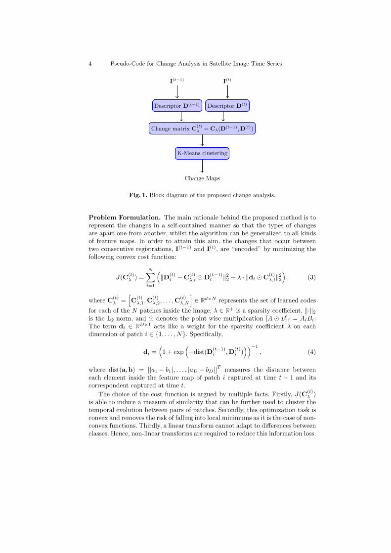
Fig. 1 summarizes the change analysis chain that was described above. Asmentioned before, throughout this paper, we bring into discussion change anal-ysis as opposed to change detection, the former being less deliberated in mostof the related papers.

3.2 Pseudo-Encoder with L2-Norm Regularization Term

Let us consider a temporal series (e.g., SITS) with T observations (e.g., satelliteimages), {I(t) ∈ RS1×S2}t∈{1,...,T}, where S1 and S2 are the dimensions of theimages. Each image is divided in N patches of size p×p pixels. At limit, the patchcan be considered of 1 pixel (i.e., p = 1). Additionally, let D(t) ∈ Rd×N containd -dimensional local descriptors (i.e., patch features, pixel values) extracted fromthe image I(t) captured at time t.


I(t−1) I(t)

Descriptor D(t−1) Descriptor D(t)

Change matrix C(t)λ = Cλ(D(t−1),D(t))

K-Means clustering

Change Maps

Fig. 1. Block diagram of the proposed change analysis.

Problem Formulation. The main rationale behind the proposed method is torepresent the changes in a self-contained manner so that the types of changesare apart one from another, whilst the algorithm can be generalized to all kindsof feature maps. In order to attain this aim, the changes that occur betweentwo consecutive registrations, I(t−1) and I(t), are “encoded” by minimizing thefollowing convex cost function:

J(C(t)λ ) =

N∑i=1

(‖D(t)

i −C(t)λ,i �D

(t−1)i ‖22 + λ · ‖di �C

(t)λ,i‖

22

), (3)

where C(t)λ =

[C

(t)λ,1,C

(t)λ,2, . . . ,C

(t)λ,N

]∈ Rd×N represents the set of learned codes

for each of the N patches inside the image, λ ∈ R+ is a sparsity coefficient, ‖·‖2is the L2-norm, and � denotes the point-wise multiplication [A � B]i = AiBi.The term di ∈ RD×1 acts like a weight for the sparsity coefficient λ on eachdimension of patch i ∈ {1, . . . , N}. Specifically,

di =(

1 + exp(−dist(D

(t−1)i ,D

(t)i )))−1

, (4)

where dist(a,b) = [|a1 − b1|, . . . , |aD − bD|]T measures the distance betweeneach element inside the feature map of patch i captured at time t − 1 and itscorrespondent captured at time t.

The choice of the cost function is argued by multiple facts. Firstly, J(C(t)λ )

is able to induce a measure of similarity that can be further used to cluster thetemporal evolution between pairs of patches. Secondly, this optimization task isconvex and removes the risk of falling into local minimums as it is the case of non-convex functions. Thirdly, a linear transform cannot adapt to differences betweenclasses. Hence, non-linear transforms are required to reduce this information loss.


Furthermore, imposing the sparsity constraint in equation (3) leads to a bet-ter separation between codes, and, thus, to a better separation between clusters,as we will see in Section 4. The sparseness is not induced using a commonL0-norm, or L1-norm, but by using the L2-norm regularization term similar tothe one proposed in [11]. This imposes the presence of few significant values inthe code, and also an analytical global solution for the minimization problem,avoiding the computational burden carried by other sparse coding methods.

The weights {di}i=1,...,N give different freedom on each dimension of the code

C(t)λ,i depending on the distance between the elements of the feature maps. In

addition, the function f(x, y) = 11+exp(−|x−y|) in expression (4) has the following

useful properties:

1. |x−y| is not sensitive to the direction of change (i.e., the distance is the samebetween feature vector at time t− 1 and those at time t, and vice-versa);

2. If |x − y| is large enough (i.e., a major change took place in the respectivearea), f(x, y)↗ 1;

3. If lim inf |x−y|→0 f(x, y) = 0.5 (i.e., no major changes).

Solution to the minimization problem. The minimization of the convex

function J(C(t)λ ) is equivalent to solving a linear system with d × N equations

and d×N unknowns, namely C(t)λ ∈ Rd×N :

−(D(t) −C

(t)λ �D(t−1)

)�D(t−1) + λ · d�

(d�C

(t)λ

)= 0.

The solution of this system of equations can be derived simply as:

C(t)λ =

D(t−1) �D(t)

D(t−1) �D(t−1) + λ · d� d, (5)

where d = [d1, . . . ,dN ] ∈ Rd×N and the division is taken element by element.

Advantages. Firstly, as already mentioned, having an analytical solution (5)to the minimization of the error function (3) represents a major advantage.

Secondly, the sparsity (i.e., of course, in the sense of fewer important values)in the codes is beneficial: It helps the clustering algorithm to distinguish betterbetween the classes, as we will see in Section 4, reducing the impact of thenoise on the data analysis, a frequent source of errors in satellite imagery (e.g.,different atmospheric conditions, different seasons between the registrations).

Furthermore, besides the direct advantages of the encoding procedure (i.e.,analytical solution, better separation), we mention also the generality of thealgorithm: the method can be applied to any type of feature maps, at a pixel-level, or patch-level, as we will show shortly.


Relation with other algebraic measures for change detection. As a firstremark, if no transform is applied to the images and λ = 0, then the pseudo-encoder is equivalent to an image rationing operation:

C(t)0 = R(t) if D(j) = I(j),∀j ∈ {t− 1, t}, (6)

where the pixel level case is considered for C(t)0 . However, image rationing is not

well-defined if the values of the pixels are close to 0, which is often the case. For

this reason, the term λ ·‖di�C(t)λ,i‖22 reduces this risk, being an added advantage

of the proposed encoding model.Moreover, the values that result by image differencing are transformed into

weights for the cost function J(C(t)λ ), which tries to equalize the importance

between the levels of change so that all changes are taken into account.

4 Experimental results

In this section, we report the results obtained by using the pseudo-encoder de-scribed in Section 3 on a challenging type of temporal series, namely satelliteimage time series (SITS). This paper uses 5 Landsat multispectral SITS cap-tured between 2001 and 2003, at 30 meters spatial resolution, covering an areaof approximately 59 × 51 km2. The satellite images are captured using six sub-bands of frequency, namely: near-infrared (NIR – the wavelengths are between0.77 – 0.90 µm) and shortwave infrared (SWIR1 and SWIR2 – the wavelenghtsare between 1.55 – 1.75 µm and 2.09 – 2.35 µm).

4.1 Feature maps

The pseudo-encoding method presented in the previous section is a general algo-rithm that can be used with any type of feature maps, depending on the desiredlevel of detail. Two cases can be depicted, namely: pixel-level, and patch-leveldescriptors.

Pixel–Level Descriptors At a given time t, for a single spectral subband,the pixel–level descriptor is built considering each pixel value, namely D(t) ∈R1×S1S2 is the vectorized form of the image, taken column by column. Themultispectral information is included by a simple concatenation of the values ofall the spectral subbands (i.e., D(t) ∈ R6×S1S2 for 6 bands).

Patch–Level Descriptors There are many types of patch based descriptorsthat describe locally the shapes and textures in an image, starting from waveletcoefficients, edge descriptors, Fourier coefficients, and so on. In this case, we willopt for local image descriptors that result from the projections onto a learnedbasis, as shown below.


Table 1. The reconstruction error of the SITS decreases with the level of detail.

Patch size MSE11 46.44 · 10−3

9 44.07 · 10−3

7 42.65 · 10−3

5 42.20 · 10−3

Let us denote by Yi ∈ Rp2×1 the column-wise form of a patch Xi ∈ Rp×p in an

image from the database. As described in [10], sparse dictionaries can be learnedstarting from n randomly selected patches from the dataset, by minimizing thefollowing convex function:

J (B, {ti}i=1,...,n) =

n∑i=1

(‖Yi −B · ti‖22 + µ · ‖ti‖1

)(7)

where B = [Bj ]j=1,...,d has the filters that compose the filterbank on each col-umn, ti are d - dimensional vectors that represent the projection of vector Yi

onto the learned dictionary B, whereas ‖·‖2 and ‖·‖1 represent the L2 - normand L1 - norm, respectively. µ models the degree of sparsity considered for therepresentation.

Table 1 shows that the mean squared reconstruction error (MSE) decreaseswith the size of the patch:

MSE =1

n

n∑i=1

1

p2‖Yi −B · ti‖22. (8)

In order to learn specific filterbanks for SITS, we considered n = 100 patchesof 7 × 7 pixels (i.e., 210 × 210 m2 covered area), D = p2 = 49, and µ = 0.5.The learned filterbanks for each spectral band of the SITS are shown in Fig. 2.The choice p = 7 is made in accordance with the analysis of change in SITS,developed in this paper. More precisely, a more detailed level of analysis (i.e., asmaller size of the patch) would lead to inconsistent detection of change, whereasa coarser one would have included different classes in the same patch, which isnot desirable.

Furthermore, the corresponding feature vector t of an arbitrary patch X,with the corresponding vector form Y, can be computed using the approximationt = BT ·Y that incorporates all the projections on the columns of the filterbankB. The feature vectors corresponding to the six subbands are concatenated,leading to a new feature vector, i.e. [tT1 , . . . , t

T6 ]T , where tl is the corresponding

descriptor that represents the lth subband of the patch in the satellite image.Under these circumstances, the length of each patch’s descriptor is 6p2.


(a) Blue filterbank (b) Green filterbank (c) Red filterbank

(d) NIR filterbank (e) SWIR1 filterbank (f) SWIR2 filterbank

Fig. 2. Learned filterbanks from SITS

4.2 Clustering the changes in SITS

Further, we perform a post-classification over the resulting pseudo-codes usingK-Means, noting that our aim is not a simple separation between “change” and“no change” as in [6] or [8], but a more complex one: The changes are groupedinto “types of changes”, that mark the transitions between the two temporalmoments.

In addition, the analysis shows that the clusters are specific to individualuser-defined classes. In order to attain this desideratum, the images are manu-ally labeled, by direct observation, as: Urban, Forest, Water, and Agriculture.For example, a change occurring in an urban environment is more likely to beincluded in an urban prototype of changes, rather than grouped with changes re-lated to water, forest, or agriculture. Moreover, these classes are time-invariant,meaning that a change doesn’t imply any kind of modification over these classes.This assumption holds for relatively short periods of time (i.e., one year in ourcase). If the analysis spans a longer period of time, the pseudo-encoder acts morelike a similarity measure, that, in conjunction with the K-Means algorithm, hasthe added capability of enhancing the separability between types of changes thata human observer cannot easily distinguish.

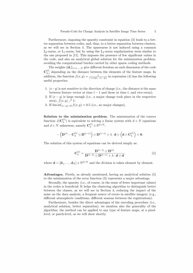
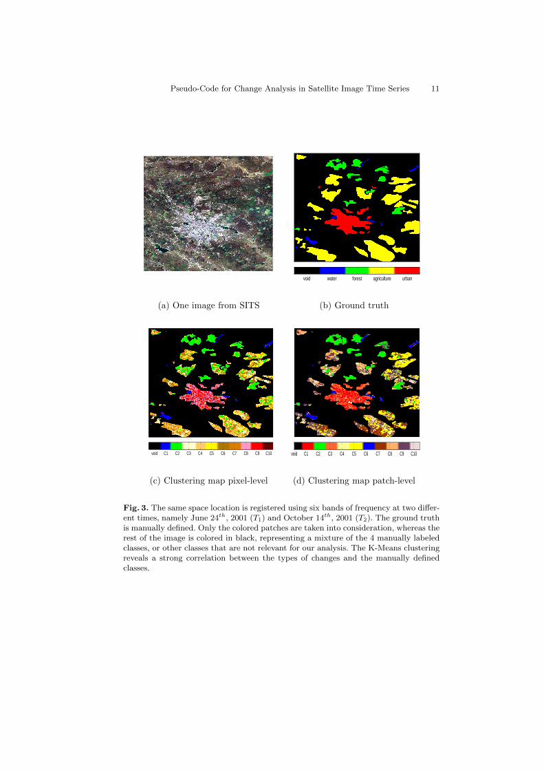
An example of 10-Means clustering is shown in Table 2, where each cluster isassigned to the class which is most frequent in the cluster. This kind of mapping,for this example in particular, can be observed in Fig. 3. The figure displays onlythe transition between June 24th, 2001 (T1) and October 14th, 2001 (T2), whilstTable 2 shows the results obtained over the 5 SITS.


Table 2. Repartition of each of the 10-Means clusters over the manually labeled classesin percentages [%]

Descriptor 10-Meansclusters

Urban Forest Water Agriculture

Pixel-level

C1 0 0 100 0C2 1.31 86.56 0.27 11.86C3 2.10 0.23 0 97.67C4 0.07 0.15 0 99.78C5 0.39 2.29 0 97.32C6 0.89 0.26 0 98.85C7 0.23 7.63 0 92.14C8 98.41 0.77 0.82 0C9 100 0 0 0C10 99.94 0 0.06 0

Patch-level

C1 99.22 0.58 0 0.19C2 0.77 86.17 12.43 0.63C3 95.78 0.32 2.00 1.90C4 1.75 2.43 2.99 92.83C5 1.03 0 1.45 97.52C6 0.34 0 98.10 1.56C7 0.67 0.91 11.72 86.70C8 0.30 0 0.30 99.40C9 6.60 2.83 10.09 80.48C10 0.80 7.40 5.39 86.41

In order to evaluate the results of our proposed method with respect tothe performance of clustering in terms of domain separation, we consider Purityand Adjusted Rand Index as the criteria for analyzing the clustering quality withrespect to the number of clusters and sparsity constraint λ. In what follows, letus denote by S = {Sj}j the manually labeled partition (i.e., user-defined classes)and, by C = {Ck}k, the resulted K-means partition.

Formally, purity [5] is defined as:

Purity =1

N

K∑k=1

maxj=1,...,|S|

|Ck ∩ Sj |, (9)

where Ck represents the kth cluster, Sj is the jth user-defined class, and |S| isthe cardinality of S. It measures the agreement between the two partitions interms of class separation. A complete agreement translates into a 100% purity,whilst independent partitions give a 0% purity.

The second criteria, Adjusted Rand Index (or, shortly ARI ), is one of themost popular performance measures for comparing two partitions of a set by


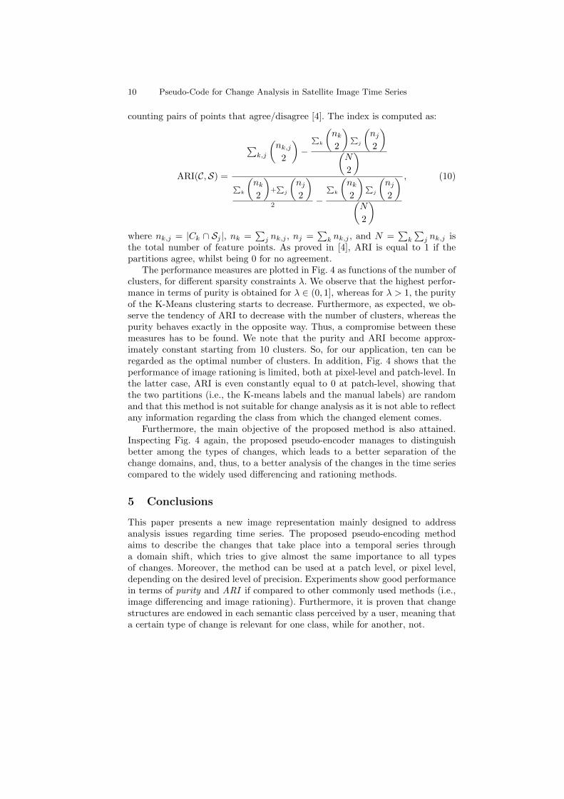
counting pairs of points that agree/disagree [4]. The index is computed as:

ARI(C,S) =

∑k,j

(nk,j

2

)−

∑k

(nk2

)∑j

(nj2

)(N

2

)∑

k

(nk2

)+∑

j

(nj2

)2 −

∑k

(nk2

)∑j

(nj2

)(N

2

), (10)

where nk,j = |Ck ∩ Sj |, nk =∑j nk,j , nj =

∑k nk,j , and N =

∑k

∑j nk,j is

the total number of feature points. As proved in [4], ARI is equal to 1 if thepartitions agree, whilst being 0 for no agreement.

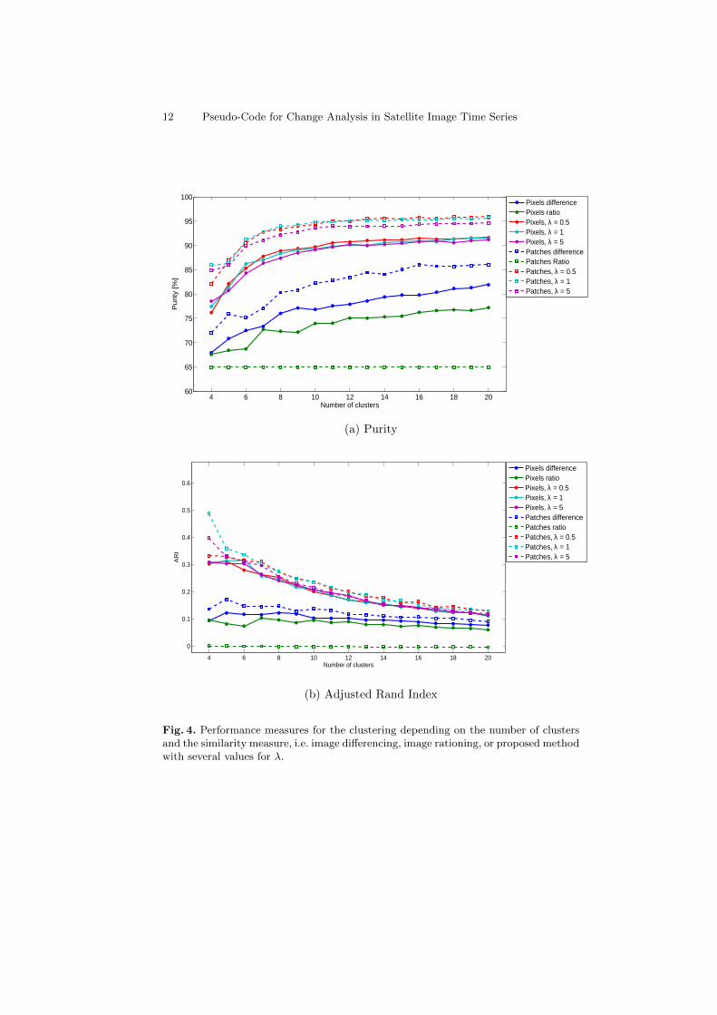
The performance measures are plotted in Fig. 4 as functions of the number ofclusters, for different sparsity constraints λ. We observe that the highest perfor-mance in terms of purity is obtained for λ ∈ (0, 1], whereas for λ > 1, the purityof the K-Means clustering starts to decrease. Furthermore, as expected, we ob-serve the tendency of ARI to decrease with the number of clusters, whereas thepurity behaves exactly in the opposite way. Thus, a compromise between thesemeasures has to be found. We note that the purity and ARI become approx-imately constant starting from 10 clusters. So, for our application, ten can beregarded as the optimal number of clusters. In addition, Fig. 4 shows that theperformance of image rationing is limited, both at pixel-level and patch-level. Inthe latter case, ARI is even constantly equal to 0 at patch-level, showing thatthe two partitions (i.e., the K-means labels and the manual labels) are randomand that this method is not suitable for change analysis as it is not able to reflectany information regarding the class from which the changed element comes.

Furthermore, the main objective of the proposed method is also attained.Inspecting Fig. 4 again, the proposed pseudo-encoder manages to distinguishbetter among the types of changes, which leads to a better separation of thechange domains, and, thus, to a better analysis of the changes in the time seriescompared to the widely used differencing and rationing methods.

5 Conclusions

This paper presents a new image representation mainly designed to addressanalysis issues regarding time series. The proposed pseudo-encoding methodaims to describe the changes that take place into a temporal series througha domain shift, which tries to give almost the same importance to all typesof changes. Moreover, the method can be used at a patch level, or pixel level,depending on the desired level of precision. Experiments show good performancein terms of purity and ARI if compared to other commonly used methods (i.e.,image differencing and image rationing). Furthermore, it is proven that changestructures are endowed in each semantic class perceived by a user, meaning thata certain type of change is relevant for one class, while for another, not.


(a) One image from SITS

void water forest agriculture urban

(b) Ground truth

void C1 C2 C3 C4 C5 C6 C7 C8 C9 C10

(c) Clustering map pixel-level

void C1 C2 C3 C4 C5 C6 C7 C8 C9 C10

(d) Clustering map patch-level

Fig. 3. The same space location is registered using six bands of frequency at two differ-ent times, namely June 24th, 2001 (T1) and October 14th, 2001 (T2). The ground truthis manually defined. Only the colored patches are taken into consideration, whereas therest of the image is colored in black, representing a mixture of the 4 manually labeledclasses, or other classes that are not relevant for our analysis. The K-Means clusteringreveals a strong correlation between the types of changes and the manually definedclasses.


4 6 8 10 12 14 16 18 2060

65

70

75

80

85

90

95

100

Number of clusters

Pu

rity

[%

]

Pixels differencePixels ratioPixels, λ = 0.5Pixels, λ = 1Pixels, λ = 5Patches differencePatches RatioPatches, λ = 0.5Patches, λ = 1Patches, λ = 5

(a) Purity

4 6 8 10 12 14 16 18 20

0

0.1

0.2

0.3

0.4

0.5

0.6

Number of clusters

AR

I

Pixels differencePixels ratioPixels, λ = 0.5Pixels, λ = 1Pixels, λ = 5Patches differencePatches ratioPatches, λ = 0.5Patches, λ = 1Patches, λ = 5

(b) Adjusted Rand Index

Fig. 4. Performance measures for the clustering depending on the number of clustersand the similarity measure, i.e. image differencing, image rationing, or proposed methodwith several values for λ.


Acknowledgments. The work has been partially funded by the Sectoral Op-erational Program Human Resources Development 2007-2013 of the Ministry ofEuropean Funds through the Financial Agreement POSDRU/159/1.5/S/134398.

References

1. J. Theau, “Change detection,” in Springer Handbook of Geographic Information,pp. 75–94. Springer Berlin Heidelberg, 2012.

2. B. Gong, F. Sha, and K. Grauman, “Overcoming Dataset Bias: An UnsupervisedDomain Adaptation Approach,” in Big Data Meets Computer Vision: First In-ternational Workshop on Large Scale Visual Recognition and Retrieval, December2012.

3. Y. Shi, and F. Sha, “Information-Theoretical Learning of Discriminative Clusters forUnsupervised Domain Adaptation,” in Proceedings of the International Conferenceon Machine Learning (ICML), 2012.

4. L. Hubert and P. Arabie, “Comparing partitions,” Journal of Classification, vol. 2,no. 1, pp. 193–218, 1985.

5. Christopher D. Manning, Prabhakar Raghavan, and Hinrich Schutze, Introductionto Information Retrieval, Cambridge University Press, New York, NY, USA, 2008.

6. T. Celik, “Unsupervised Change Detection in Satellite Images Using Principal Com-ponent Analysis and k -Means Clustering,” IEEE Transactions on Geoscience andRemote Sensing, vol. 6, no. 4, pp. 772–776, 2009.

7. L. Bruzzone, D.F. Prieto, “Automatic analysis of the difference image for unsuper-vised change detection,” IEEE Transactions on Geoscience and Remote Sensing,vol. 38, no. 3, pp. 1171–1181, 2000.

8. Y. Zheng, X. Zhang, B. Hou, G. Liu, “Using Combined Difference Image and K-Means Clustering for SAR Image Change Detection,” IEEE Geoscience and RemoteSensing Letters, vol. 11, no. 3, pp. 691–695, 2014.

9. C. Vaduva, T. Costachioiu, C. Patrascu, I. Gavat, V. Lazarescu, and M. Datcu, “Alatent analysis of earth surface dynamic evolution using change map time series,”IEEE Transactions on Geoscience and Remote Sensing, vol. 51, no. 4, pp. 2105–2118, 2013.

10. B. A. Olshausen and D. J. Field, “Sparse coding with an overcomplete basis set:a strategy employed by v1,” Vision Research, vol. 37, pp. 3311–3325, 1997.

11. J. Wang, J. Yang, K. Yu, F. Lv, T. Huang, and Y. Gong, “Locality-constrainedlinear coding for image classification,” in IEEE Conference on Computer Visionand Pattern Recognition (CVPR), June 2010, pp. 3360–3367.

Documents

A L2-Norm Regularized Pseudo-Code for Change Analysis in ... · A L2-Norm Regularized Pseudo-Code for Change Analysis in Satellite Image Time Series Anamaria Radoi1;2 and Mihai Datcu3