A Hybrid Discrete Choice Model of Differentiated ProductDemand with An Application to Personal Computers

Minjae Song∗

Simon Graduate School of Business, University of Rochester

May 2012

Abstract

In this paper I consider a new discrete choice model of differentiated product demand thatdistinguishes a brand-level differentiation from a product-level differentiation. The model is ahybrid of the random coeffi cient logit model of Berry, Levinsohn, and Pakes (1995) and thepure characteristics model of Berry and Pakes (2007). This hybrid model describes marketswhere firms offer multiple products of different qualities under the same brand name. I showthe advantages of using the hybrid model in such markets using Monte Carlo simulations as wellas product-level data on personal computers. Using the estimates of the hybrid model, I alsoprovide empirical evidence that firms reposition their brands in a post-merger market.

JEL classification numbers: C51, D43, L13, L63Keywords: Discrete choice models, product differentiation, personal computer market,

post-merger analysis

∗Please send your comments to minjae.song@simon.rochester.edu. I have benefited from discussions with AnaAizcorbe, Yuk-Fai Fong, Maurizio Iacopetta, Sarit Markovich, Aviv Nevo, Robert Porter, and participants at variousseminars and conferences. I especially thank Bureau of Economic Analysis for providing me with data used in thispaper. Yang Lin and Mark Yuan provided excellent research assistance. All errors are mine.

1

1 Introduction

Consider a market where brands compete with multiple products, and products of a given brand

can be ranked with respect to product characteristics. The auto market is a good example. There

are different brands of cars, and each brand has a low-end economy car, a mid-range car, and a

high-end luxury car. The computer market is another example. Products of each brand range

from computers of a low CPU speed with low memory and hard disk capacities to computers of a

high CPU speed with large memory and hard disk capacities. In such markets each brand targets

“high-end" consumers with high quality and high price products and “low-end" consumers with

low quality and low price products.

In this paper I consider a new discrete-choice model of differentiated product demand

in which product groups are “horizontally" differentiated while products of a given group are

“vertically" differentiated with respect to observed characteristics. I call a product group that

contains “vertically" differentiated products a brand. This is consistent with the role of brands

found in many markets. In my model products of the same brand are not necessarily ranked on

the single dimension. In the car market case, for example, it is not straightforward to compare

SUVs with sports cars on the single quality dimension. My model can accommodate this case by

allowing consumers to differ in multiple dimensions. In the car example, consumers may value the

car size differently but agree on the quality ranking conditional on the size.

I distinguish these two types of differentiation by assuming that consumers receive an

idiosyncratic shock only at a brand level so that all products within a brand share the same shock.

This shock represents each consumer’s idiosyncratic "taste" for a brand that is not captured by

observed and unobserved product characteristics, and I assume that it is independent and identically

distributed with Type I extreme value distribution. As a result, consumers’product choice within

a brand is solely determined by their preference for product characteristics, and their brand choice

is determined by the realization of the brand-level shock in addition to the preference. The model

has at least one random coeffi cient that describes heterogeneous consumer preferences. With one

random coeffi cient, for example, consumers endowed with different degrees of willingness to pay for

2

overall product quality know for sure which product to choose in each brand, and choose among

those products after the taste shock for brands is realized.

I call this model a hybrid model because it resembles the random coeffi cient logit demand

model in describing a brand choice (Berry, Levinsohn, and Pakes 1995; BLP hereafter) and the

pure characteristics demand model in describing a within-brand product choice (Berry and Pakes

2007; the PCM hereafter). For the markets described above the hybrid model provides a more

realistic substitution pattern than the existing demand models. Since the within-brand product

choice is not affected by the idiosyncratic shock, only a subset of products are substitutes for one

another within a brand and these substitutes are similar in their characteristics. Yet, all brands

are substitutable as each brand has one of the products that consumers choose from.1 This is

an important feature for the aforementioned markets where firms compete to attract each type of

consumer with products of different qualities.

Another important feature is that the hybrid model distinguishes brand entry from product

entry. New products introduced by existing brands do not add idiosyncratic shock, while new prod-

ucts by a new brand add one brand-level shock. As a result, consumer welfare does not necessarily

grow by adding more products. This is in contrast to models with product-level idiosyncratic shock

such as BLP where consumer welfare grows without a bound as the number of products increases.

One should note that my hybrid model is different from the nested logit model. The

two models are similar in that both divide products into groups and distinguish within-group

substitution from cross-group substitution. However, the nested logit model does not accommodate

non-idiosyncratic consumer types. As a result, the choice probabilities for groups and products

within a group are determined by the average utility the consumer receives. On the other hand,

in the hybrid model each consumer has a different group choice probability that is determined by

her type and chooses a product within a group solely based on her type. Also, while grouping is

arbitrary in the nested logit model, the hybrid model requires that each group have a (conditional)

quality ranking.

One should also note that the hybrid model is different from the PCM with random coeffi -

1All products are substitutes to one another in BLP and all brands are not necessarily substitutable in the PCM.

3

cients on the brand dummy variables.2 In the hybrid model the brand-level shock is idiosyncratic,

so all consumers have a positive probability of choosing any brand, which makes all brands substi-

tutable for one another. On the other hand, a random coeffi cient on the brand dummy represents

(non-idiosyncratic) consumer types, so only consumers endowed with high values of the random

coeffi cient choose that brand, which makes brands less substitutable.3

Using Monte Carlo simulations I show how the hybrid model is different from the existing

models such as BLP and the PCM. Rather than choosing the hybrid model as a true model, I use

all of the three models as a true model one at a time and estimate the other two models. All models

have the common feature that multiple brands (firms) compete with multiple products and prices

are set according to their within-brand quality ranking. Depending on which model is chosen as a

true model, the idiosyncratic error structure differs and, hence, simulated market shares differ as

well.

Simulation results show that the hybrid model is more robust to the (mis-)selection of

models. Comparing the hybrid model and BLP, the mean square errors of the hybrid estimates

(when BLP is treated as a true model) are about one third of those of the BLP estimates (when

the hybrid model is a true model). The BLP estimates are close to true values on average but their

variances are much larger, resulting in larger MSEs. However, both the hybrid model and BLP

perform equally poorly when the PCM is a true model and the PCM performs poorly when either

of the two models is a true model.

The results on the markup and consumer welfare show that the model structure deter-

mines their magnitudes while the choice of a true model only has marginal impact. For example,

the PCM’s markup is drastically lower than those of the other two no matter which model is chosen

as a true model. They also show that, despite much higher own-price elasticity, the hybrid model’s

markup prediction is not substantially different from that of BLP. This is because close substitutes

belong to the same brand and the brand-level taste renders the degree of the cross-brand substitu-

tion not much different from that of BLP. Yet, the welfare effects of new products introduced by

existing brands are similar to those of the PCM because the welfare contribution of the taste term

2See Song (2007) for an example of how the PCM with two random coeffi cients is used to estimate demand.3 It may not be computationally feasible to include the random coeffi cients for all brands in the PCM.

4

is limited to the brand level.4

I also show the advantages of using the hybrid model in a real world application by es-

timating demand for desktop personal computers (PCs).5 I use monthly product-level data over

three years starting from October 2001. The data set covers about 60 percent of PCs sold at U.S.

retail stores. Data on prices, sales in unit, and ten product characteristics are available at a UPC

bar code level. There are six brands included in the data: Sony, Hewlett-Packard (HP hereafter),

Gateway, Compaq, eMachines and Apple.

Previous studies on PC demand use BLP-type models with much more aggregate data. For

example, Chu, Chintagunta and Vilcassim (2007) define a desktop PC as a brand-model-CPU type

combination. Goeree (2008) defines it as a brand-model-CPU type-CPU speed combination. These

data formats eliminate the quality ranking within brands such that products are presented as much

more horizontally differentiated than they actually are. An exception is Bajari and Benkard (2005)

who use the same product-level data I use here. Their model is similar to the PCM in that it does

not have the idiosyncratic taste shock, but more flexible in a sense that they do not make any

distributional assumption on the random coeffi cient for product characteristics. However, they can

only set-identify preference, and their demand estimates cannot be used to learn about supply-side

parameters such as the marginal cost and markup.

Estimation results show that in the hybrid model almost all coeffi cients on product char-

acteristics are statistically significant and have expected signs and reasonable magnitudes. The

random coeffi cient on the price variable is also statistically significant, which is especially en-

couraging because no individual-level data such as the current population survey or the consumer

expenditure survey is used in estimation. On the other hand, in BLP no coeffi cient other than those

on the CPU speed and the DVD Writer is statistically significant. Although the demand estimates

in the PCM are statistically significant and have expected signs, the consumer’s willingness to pay

for quality improvement is unrealistically low. For example, the average consumer is willing to pay

4Song (2010) shows that the price index based on the PCM is comparable to the standard dummy variable hedonicprice index as well as the Pakes index in Pakes (2003).

5Other researchers have adopted my model for various applications. Byzalov (2010) applies the hybrid modelto the cable TV market and finds that it fits data better than the PCM and gives more reasonable predictionsin counterfactual exercises than BLP. Ghose, Ipeirotis, and Li (forthcoming) apply the hybrid model to the hotelindustry and find that it outperforms the nested logit and BLP in out-of-sample predictions.

5

about $30 to increase CPU speed by 1 GHz. This is much less than the money needed to put a

1 GHz faster CPU. This low magnitude is a result of ignoring the brand-level differentiation and

ranking all products on the single quality dimension. In the hybrid model the average consumer’s

willingness to pay for the same CPU speed difference is about $200.

Estimated markup and consumer welfare confirm the findings in the Monte Carlo exercises.

In addition, the markup level is reasonable (lower than 30 percent) in the hybrid model when

potential consumers are included in defining the market, while it is consistently unrealistically

high in BLP (higher than 50 percent) and unrealistically low in the PCM (lower than 1 percent).

As expected, consumer welfare is less sensitive to new product introduction than in BLP, but

surprisingly it is less sensitive than in the PCM as well. This is because in the PCM consumers

who buy new products have much higher willingness to pay as the new products are positioned on

the far left end of the random coeffi cient distribution.

Lastly, I show how demand estimates can be used to analyze product repositioning in the

post-merger market. In particular, I analyze the PC market after the merger between HP and

Compaq, which took place in February 2002. The price gap between HP and Compaq was less

than $100 right before the merger but reached about $300 by the end of the sample period mainly

due to Compaq’s price decline. This price trend is not consistent with the usual prediction that

the merged firm will increase prices, at least relative to those of non-merged firms, by exploiting

its market power.

To see if this post-merger market trend is associated with product repositioning, I construct

a quality index for each brand using the demand estimates in the hybrid model. This index is a linear

function of observed product characteristics with each characteristic weighted by the estimated

marginal utility. Having statistically significant estimates with realistic magnitudes is important

in correctly projecting product positioning on characteristics space. The trend of the quality index

shows that Compaq’s quality improves more slowly than that of HP such that their difference

becomes increasingly larger over time. Moreover, Compaq’s quality becomes almost identical to

that of eMachines from July 2003, suggesting that Compaq now competes with eMachines at the

low end of the market. This provides the evidence that the merged firm repositioned Compaq and

6

HP by including more low-end products in Compaq’s product line.

The rest of the paper is organized as follows. Section 2 describes the hybrid demand

model, followed by an estimation procedure in section 3. Section 4 uses Monte Carlo simulations to

compare the hybrid model with BLP and the PCM. Section 5 estimates demand for PCs. Section

6 analyzes the post-merger PC market. Section 7 concludes.

2 Hybrid Demand Model

2.1 Utility Function

Suppose there are t = 1, 2, ..., T markets with K brands. Each brand has Jk products that are

ranked on a single quality dimension, ie., vertically differentiated. Products of the same brand do

not have to be vertically differentiated. The model I present below becomes more general by adding

more random coeffi cients, but I will confine my exposition to the simplest case. Each market has

i = 1, 2, ..., It consumers. Given a market, the indirect utility of consumer i from product j of

brand k is

uijk = δjk − αipjk + εik, for 1 ≤ jk ≤ Jk and 1 ≤ k ≤ K (1)

where δjk and pjk are quality and price of product j of brand k respectively, αi is the individual-

specific price coeffi cient with αi ∼ F (θ), and εik is consumer i′s idiosyncratic taste for brand k

which is assumed to be a Type I extreme-value random variable. Note that εik is independent and

identically distributed across consumers and brands, but not across products of the same brand.

This means that consumers receive an idiosyncratic taste shock when they consider which brand

to choose, but have the same shock for products of the same brand.

I assume that product quality δjk is a linear function of product characteristics so that

δjk = xjkβ + ξjk

where xjk is a vector of observable characteristics of product j of brand k, β represents a marginal

7

utility that a consumer derives from product characteristics, and ξjk is the mean quality of char-

acteristics that the consumer observes but the econometrician does not. In a more general version

of the hybrid model a subset of β can be random variables to describe consumer heterogeneity in

multi-dimensions.

2.2 Market Share

A rational consumer with a value of αi chooses brand k over other brands if and only if

maxjk∈k

(δjk − αipjk) + εik > maxjr∈r

(δjr − αipjr) + εir, ∀r 6= k.

Within brand k consumer i chooses product j if and only if

δjk − αipjk > δhk − aiphk , ∀hk 6= jk.

Thus the probability of brand k being chosen is

Pr (brand k being chosen) =

∫exp (maxjk∈k (δjk − αipjk))∑Kr=1 exp (maxjr∈r (δjr − αipjr))

f (α) dα, (2)

and the probability of product j being chosen conditional on brand k being chosen is

Pr (j being chosen |k being chosen) = F(4jk

(δk, pk) |θ)− F

(4jk

(δk, pk) |θ), (3)

where F (.) is the cdf of αi, 4j (δk, pk) =δjk−δj−1kpjk−pj−1k

, and 4jk

(δk, pk) =δj+1k−δjkpj+1k−pjk

with products in

each brand sorted in the order of ascending price. Note that the probability of the brand choice

also depends on the consumer’s product choice within each brand through a max function.

The market share of product j of brand k is

sjk =

∫αi∈jk

exp (δjk − αipjk)∑Kr=1 exp (maxjr∈r (δjr − αipjr))

f (α) dα

where αi ∈ jk indicates consumers who choose product j in brand k. Note that there is no max

8

function in the numerator. This share function can be rewritten as the product of the probability

in equation (3) and the probability that brand k is chosen by those consumers who buy product j

of brand k. That is,

sjk =[F(4jk

(δk, pk) |θ)− F

(4jk

(δk, pk) |θ)] ∫

αi∈jk

exp (δjk − αipjk)∑Kr=1 exp (maxjr∈r (δjr − αipjr))

g (α) dα

(4)

where

g (α) =f (α)[

F(4jk

(δk, pk) |θ)− F

(4jk

(δk, pk) |θ)] ,

and its numerical approximation is

s̃jk =[F(4jk

(δk, pk) |θ)− F

(4jk

(δk, pk) |θ)] 1

ns

∑i∈jk

exp (δjk − αipjk)∑Kr=1 exp (maxjr∈r (δjr − αipjr))

,

where ns is the number of simulated consumers whose α ∈[4jk

(δk, pk) ,4jk(δk, pk)

). The market

share function shows why the model is a hybrid model. By limiting the idiosyncratic taste shock

at a brand level, the model combines the choice probabilities of the PCM and BLP.

The random coeffi cient captures heterogeneous consumer preferences in product charac-

teristics. In this particular model, a value of αi determines which product to choose within each

brand. A consumer with a low value of αi chooses a high quality product (almost equivalently, an

expensive product) within brands and a consumer with a high value chooses a low quality product.

In equation (4) consumers endowed with α ∈[4jk

(δk, pk) ,4jk(δk, pk)

)choose product j of brand

k for sure, given that they choose brand k.

However, their brand choice is stochastic because of the brand-level idiosyncratic shock, and

is described by the integral part in equation (4) . There is a product in each brand that maximizes

the utility of a consumer endowed with α and the brand-choice probability for this consumer is a

function of these products. This means that even consumers who choose the same product of a

certain brand can have different brand-choice probabilities as the utility-maximizing products of

other brands can differ. In equation (4) this is determined by the max function in the denominator

9

of the integral part. This also means consumers who choose the same product of a certain brand

may switch to different products of another brand depending on their values of α.

As a result, a product has fewer substitutes than in BLP but more substitutes than in

the PCM, and these substitutes are similar in their quality as consumer types determine which

products are substitutes. This is a realistic description of many markets, including the PC market

where consumers rarely switch to very low-end products when the price of a very high-end product

goes up.

Equation (4) also shows how the hybrid model distinguishes the within-brand quality (ver-

tical) differentiation from the brand-level differentiation. With one random coeffi cient, as in this

specification, prices determine the quality ranking within a brand, meaning that δjk > δhk if

pjk > phk . The brand-level differentiation is horizontal in a sense that all brands are substitutes

for one another, but can still reflect brand-level quality differences. Since the random coeffi cient

determines the utility-maximizing product of each brand, it is possible that one brand’s low-end

product is a substitute for another brand’s high-end product.

The hybrid model accommodates two types of the outside option. One is to choose the

lowest quality product in each brand, and its value is set to zero.6 Consumers whose αi is very high

choose this outside option. This is the same outside option used in the PCM. The other outside

option is to choose brands that are not included in the sample or to not choose any products, and

its market share is determined by how the market is defined. Instead of setting its value to zero, it

can be excluded as in equation (4) or its value can be estimated if included. When included, the

denominator inside the integral in equation (4) becomes

exp (δ0) +

K∑r=1

exp

(maxjr∈r

(δjr − αipjr)),

where δ0 is estimated. For example, I do not have data on Dell products as the data were collected

from retail stores. Instead of ignoring them, I include it in the outside option and estimate the

average value of choosing Dell products. More details are provided in section 5.2.

6The zero value assumption does not mean that there is no systematic quality difference across brands. See Section3 for details.

10

2.3 Price Elasticity

The own-price elasticity of demand is

∂sjk∂pjk

pjksjk

=pjksjk

∂

∂pjk

(∫αi∈jk

exp (δjk − αipjk)∑Kr=1 exp (maxjr∈r (δjr − αipjr))

f (α) dα

)

=pjksjk

(Ψ(4jk

)f(4jk|θ) ∂4jk

∂pjk−Ψ

(4jk

)f(4jk|θ) ∂4

jk

∂pjk

)

+pjksjk

(∫αi∈jk

−αiΨ (αi) (1−Ψ (αi)) f (α) dα

)(5)

where

Ψ (αi) =exp (δjk − αipjk)∑K

r=1 exp (maxjr∈r (δjr − αipjr)).

Equation (5) shows that the own-price elasticity equation consists of two parts. The term in the

first bracket captures changes in market share due to substitution among products of the same

brand, and the term in the second bracket captures changes due to substitution across brands. The

former resembles the own elasticity in the PCM, but is a function of products of the same brand

and is weighted by Ψ(4jk

)and Ψ

(4jk

). The latter resembles the own elasticity in BLP, but only

a subset of consumers is considered such that −αiΨ (αi) (1−Ψ (αi)) is integrated over consumers

who buy product j of brand k.

There are two types of cross-price elasticity: within-brand cross elasticity and cross-brand

elasticity. Within-brand cross elasticity measures the impact of price changes on products of the

same brand, while cross-brand elasticity measures the impact of price changes on products of

different brands. The former is defined as

∂sjk∂phk

phksjk

=phksjk

∂

∂phk

(∫αi∈jk

exp (δjk − αipjk)∑Kr=1 exp (maxjr∈r (δjr − αipjr))

f (α) dα

)

=phksjk

(Ψ(4jk

)f(4jk|θ) ∂4jk

∂phk−Ψ

(4jk

)f(4jk|θ) ∂4

jk

∂phk

), (6)

where ∂4jk/∂phk

(or ∂4

jk/∂phk

)is zero if 4jk

(or 4

jk

)is not a function of phk . The latter cross

11

elasticity is defined as

∂sjk∂phm

phmsjk

=phmsjk

∫αi∈jk

αi exp (δjk − αipjk) exp (δhm − αiphm)[∑Kr=1 exp (maxjr∈r (δjr − αipjr))

]2 f (α) dα

(7)

if (δhm − αiphm) = arg maxjm (δjm − αipjm) for αi ∈ jk. If not, ∂sjk/∂phm = 0.

Equations (4) ∼ (7) show that when the price of a given product changes it affects products

of the same brand in its adjacent neighborhood as well as the products of different brands of a

similar quality. This is an important difference from other discrete choice models. For example,

in the PCM with one random coeffi cient a price change only affects products in a given product’s

adjacent neighborhood of the quality ranking. In any sort of logit demand model, it affects all other

products in the market. The functional form of these equations also shows that the degree of the

within-brand substitution is larger than that of the cross-brand substitution, and this is confirmed

in the Monte Carlo simulation in section 4. This means that products of the same brand are much

closer substitutes than products of different brands.

As shown in sections 4 and 5, despite these differences in the substitution pattern, estimated

markup in the hybrid model is not much lower than that of BLP because the degree of the cross-

brand substitution is not drastically different between the two models. However, the markup is

more responsive to the market size in the hybrid model such that the markup level goes down to

a realistic level when the market is defined to include potential consumers. A larger market size

does not have much impact on the second part of equation (5) but increases the magnitude of the

first part through a smaller sjk , and thus increases the own-price elasticity. An intuition for the

larger impact on the first part is as follows. When the market size becomes larger by including

more potential consumers, it does not affect how many of the existing consumers switch to the

same-brand products from a price increase. However, this same change is now larger relative to the

decreased market share, resulting in a larger percentage change.

12

2.4 Consumer Welfare

Consumer welfare of a consumer with a value of αi, converted into a monetary unit, is given as

ln(∑K

k=1 exp (maxjk∈k (δjk − αipjk)))

αi. (8)

The summation in the numerator is over brands, not over all products in the market, and there is

a maximum function inside the exponential function. The model links the consumer to a product

in each brand that maximizes her utility, and computes her welfare over products of her choice in

each brand. This implies that when firms introduce new products that are better than the existing

products, their welfare contribution is limited to a subset of consumers whose willingness to pay for

quality improvement is high. The equation also shows that the overall welfare grows more slowly

than that of models with the product-level taste term. The average consumer welfare is given as

∫ ln(∑K

k=1 exp (maxjk∈k (δjk − αipjk)))

αidF (α) (9)

Note that, as the value of αi changes, a product choice within brands also changes by the maximum

function.

3 Estimation

I use a non-linear GMM estimation to estimate the model. Given parameter values, I search

for a vector of product quality, δ, such that the model-predicted market shares equate observed

market shares. Then I compute a GMM objective function using the moment condition that the

mean of unobserved characteristics is uncorrelated with instrumental variables. By repeating this

for different parameter values, I find a set of values that minimizes the GMM objective function.

Parameters to estimate are the coeffi cients of product characteristics and the parameters for the

distribution of α.

A computational challenge lies in finding product quality, δ, that matches the model-

13

predicted market shares with observed market shares. The Newton-Raphson method is a natural

candidate for this type of problem. For each market there are∑K

k=1 Jk number of nonlinear

equations, which is equal to the number of products, and∑K

k=1 Jk variables, a vector of product

quality. In my experience this method works well when the number of products per market is less

than twenty. When the number of products is higher, it is important to have good starting values.

However, when there are more than fifty products per market, the computational time increases so

much that it becomes impractical.

Thus, for markets with more than fifty products, I developed a more practical yet theoreti-

cally valid method. The key idea is to use a product’s observed within-brand share to approximate

the conditional probability of choosing a product within a brand.7 My method consists of two steps.

In the first step, the quality of the lowest quality product in each brand is set to an arbitrary value,

and the qualities of the other products are computed by equating (observed) within-brand shares to

equation (3). The second step searches for the quality of the lowest quality product in each brand

by equating observed brand shares to equation (2) . The first step is the same procedure used in

the PCM and the second step is the Newton-Raphson method with the number of roots equal to

the number of brands. In the one random coeffi cient hybrid model, the first step’s computational

burden is trivial as inverting equation (3) is straightforward.8 The second step takes longer, but

the computational burden is rarely prohibitive as the number of brands is usually far smaller than

the number of products.

This method always finds the unique δ with one random coeffi cient. The existence and

uniqueness of δ can be established using the proof in Berry (1994) . Because the first step uses the

inversion of the market share function, all I need to show is that the quality of the lowest quality

product uniquely exists in the second step. The suffi cient conditions for existence in Berry (1994)

7A similar idea is used in Berry (1994) to estimate a nested logit demand model.8For product j of brand k,

δjk = δj−1k + (pjk − pj−1k )F−1

(1−

j−1k∑r=0

s̃r|θ)

where F is the cdf of the log normal distribution and s̃r is the within-brand market shares. Note that in the tworandom coeffi cient hybrid model the computational burden increases substantially in the first step as this inversionis no longer possible.

14

are that the market share function, s (δ) , is everywhere differentiable with respect to δ, and its

derivatives obey the following strict inequalities.

∂sjk∂δjk

> 0

∂sjk∂δk

< 0 for k 6= jk.

Notice that the second inequality is not satisfied if all products are not necessarily substi-

tutes for one another. However, they are satisfied with the brand share function. Let sk be the

brand share function.

sk (δ1) =

∫exp (maxjk∈k (δjk (δ1k)− αipjk))∑Kr=1 exp (maxjr∈r (δjr (δ1r)− αipjr))

f (α) dα

where δ1 is a vector of the lowest quality product in each brand. Notice that δjk and δjr are

functions of δ1k and δ1r respectively. It is straightforward to show that

∂sk∂δ1k

> 0

∂sk∂δ1r

< 0 for r 6= k.

Therefore, it follows that δ1 exists such that sk (δ1) equals brand k′s market share for all k. Once

the existence is established, the uniqueness follows from the property that increasing all the mean

product quality, including the within-brand outside option, by the same amount does not change

any brand market share.

Note that researchers do not usually have data on brand-level shares that include the

within-brand outside option. In that case, they can match∑Jk

jk=1sjk to

(1− s̃0k (δ1))

∫exp (maxjk∈k (δjk (δ1k)− αipjk))∑Kr=1 exp (maxjr∈r (δjr (δ1r)− αipjr))

f (α) dα

where s̃0k is the within-brand market share of the outside option and determined by 1−F (δ1k/p1k |θ),

15

given δ1k and θ.9 Alternatively, one may compute the model-predicted market share for each prod-

uct given the product quality recovered in the first step, and sum them up for each brand to match

it to∑Jk

jk=1sjk . This method gives similar results for the data used in this paper but is slower since

it needs to compute individual product shares.

The GMM estimator in the one random coeffi cient hybrid model belongs to the class of es-

timators that Berry, Linton, and Pakes (2004) consider. The share function in equation (4) satisfies

their regularity conditions, and the share function simulator is the same as theirs. Therefore, their

results on the consistency and the asymptotic normality (Theorems 1 and 2) can be applied directly.

However, they do not formally provide asymptotic properties for the multi-dimensional pure char-

acteristics model. Instead, they explain why it is not likely to differ from the unidimensional model,

and support their argument with Monte Carlo simulations. I expect the multi-random coeffi cient

hybrid model to share the same asymptotic properties as the multi-dimensional pure characteristics

model, but leave a formal proof for future research.

Simple examples may help the reader understand how the hybrid model uses prices and

market shares to infer product quality. Suppose there are two brands with each brand having two

(vertically differentiated) products. Suppose further that the price of Brand 1’s low-end product is

the same as the price of Brand 2’s high-end product, ie.,

p1,high > p1,low = p2,high > p2,low

and

p1,high − p1,low = p2,high − p2,low

Note that the outside option here is to choose another product in each brand that we do not data

on and its utility is set to zero. First, assume that all four products have the same market shares.

Then it should hold thatδ1,lowp1,low

=δ2,lowp2,low

9∑Jkjk=1

sjk =∑Jk

jk=1qjk/M = (1− s̃0k )

∑Jkjk=0

qjk/M

16

andδ1,high − δ1,lowp1,high − p1,low

=δ2,high − δ2,lowp2,high − p2,low

Because p1,low > p2,low, it follows that δ1,low > δ2,low, and thus δ1,high > δ2,high. This implies that

Brand 1 can charge higher prices and still have the same market shares because the quality of their

products is higher.

Now suppose the market share of Brand 1 products is larger than that of Brand 2 products.

This will make the difference between δ1,low and δ2,low even larger, which is consistent with the

economic logic that if more consumers choose a more expensive brand, its quality must be so much

higher. It is also easy to see that the quality difference will be smaller as Brand 1’s share becomes

smaller. It is even possible that δ1,low < δ2,low if the market share of Brand 1 is substantially

smaller than that of Brand 2. It is not surprising that a brand with higher prices and lower quality

attracts much fewer consumers. These examples also show that the zero utility normalization for

the outside option does not mask the systematic quality differences across the brands.

4 Model Comparisons Using Monte Carlo Simulation

In this section I use Monte Carlo simulations to compare the hybrid model with BLP and the PCM.

The purpose of this section is to provide researchers and practitioners with guidelines on model

selections. I compare the models on three dimensions. First, I generate market shares in the three

models and compare them. All three models have the same product quality and prices, so any

differences in market shares come from the idiosyncratic error structure. Second, I take one of the

three models as a “true" model one at a time and use its market shares to estimate the other two

models. For example, when BLP is treated as a “true" model, I use the market shares generated by

BLP and estimate the PCM and the hybrid model. Third, I repeat the second exercise to compute

markups and consumer welfare, using both the “true" and the estimated demand parameters.

When I use BLP shares as true shares, for example, the true demand parameters are those of BLP

and the estimated demand parameters are those of the other two models estimated in the second

exercise. This way I show to what extent the differences in markups and consumer welfare are

17

attributed to differences in the error structure or in the parameter values.

4.1 Market Shares

In a market there are three brands with each brand having four products. There is one observable

attribute, x, and I assume that this attribute is a desirable characteristic and distributed uniformly

on (0, 1). There are brand dummy variables, γ = [γ1, γ2, γ3] , that capture the average utility of

brand-level unobserved attributes, and I set γ = [1, 0.5, 0]. I assume that price is an exponential

function of the mean product quality which is a linear combination of the observable attribute and

the brand dummies. Thus, the price of product j of brand k is

pjk = c exp (β0 + β1xjk + γk)

where I set c = 1/20, β0 = 2 and β1 = 1.5.

I allow for an unobservable attribute, ξjk but do not allow it to be correlated with the price

to make estimation simple. Thus, the price endogeneity problem is absent in this exercise. I assume

that ξjk ∼ 0.001×N (0, 1) . The small variance provides two benefits. First, the number of markets

required for consistent estimation is small. The estimates of the “true" model are no different from

true values with ten independent markets (120 products in total). Second, the smaller variance of

ξjk, the easier it is to generate positive market shares in the hybrid model and especially in the

PCM.

Consumers are heterogeneous on a single dimension and the heterogeneity, denoted by αi,

is captured by a random coeffi cient on the price variable. I assume that log (α) ∼ N (µ, σ) where

(µ, σ) = (0, 1) . In all models I fix µ at 0 and treat σ as a parameter to estimate. Let Uijk be the

component of the utility function that all of the three models share,

Uijk = δjk − αipjk

where δjk = β0+β1xjk+γk+ξjk. Despite being simple, this utility function describes many markets

including the PC market where multiple brands compete with vertically differentiated products.

18

Given this common component, each model generates different market shares because of

the different structure of the idiosyncratic error term. Table 1 summarizes the brand-level as well

as the product-level market shares that each model generates over 100 repetitions. I compute the

mean and the standard deviation across ten markets for each repetition and report their averages

across 100 repetitions. For each brand, product 1 is the lowest quality and product 4 is the highest

quality product.

First, note that in BLP market shares are more evenly distributed across the quality ranking

and the product-level standard deviations are smaller. Because of the product-level idiosyncratic

shock, the quality difference and consumer heterogeneity is less important in generating market

shares. Also, note that the standard deviation is much larger in the PCM at both brand- and

product-level. In the PCM all products are ranked on the single quality dimension, and the most

expensive and the least expensive products have substantially larger market shares because they

have one less substitute, resulting in the large product-level standard deviation. Since any brand

can have these products, the brand-level standard deviation is also large. In the hybrid model, the

most expensive and the least expensive products of each brand have larger market shares, resulting

in smaller standard deviations.

4.2 Parameter Estimation

Table 2 shows estimation results when one of the three models is treated as a “true" model. Under

the heading Hybrid, for example, a true model is the hybrid model so all models use the market

shares generated in the hybrid model.10 This exercise shows how close estimates are to true values

when a model is mis-specified. I use the method of moments for estimation. Since µ is fixed and

the price variable is not correlated with ξ, the number of moments is the same as the number of

parameters. I use the grid search for the price parameter, σ, as it enters the model non-linearly.

The table shows that the hybrid model is closer to BLP than to the PCM with respect

to the mean square error. Both the hybrid model and BLP do poorly when the PCM is a true

model. Their estimate for σ is far above the true value and the MSEs for all parameters are the10The estimates of the “correct" model (e.g., the hybrid model estimated with the hybrid market shares) are very

close to the true values so I put the true values instead.

19

largest than in any other cases. When either of the hybrid model or BLP is a true model, the PCM

substantially underestimates σ but estimates the brand parameters, γ, closer to the true values

than the other two models do.

Between the hybrid model and BLP, the hybrid estimates are more robust with respect to

the model (mis-)selection. Their means are very close to the true values, and their mean square

errors are one third of those of the BLP estimates for almost all parameters. The BLP estimates

are close to the true values on average, but their variances are much larger, resulting in much larger

MSEs.

4.3 Markup and Welfare

Next I calculate the markup using the estimation results in table 2. In table 3 I report the absolute

markup for Products 1, 2, 3, and 4 averaged across the brands. Both the mean and the standard

deviation are computed across the markets and then averaged over 100 repetitions.

Table 3 first shows that the markup is similar between the hybrid model and BLP, no

matter which market shares (and demand estimates) are used. The latter model tends to have

larger markups for Products 3 and 4, but the differences are small.11 This is interesting, considering

their differences in the substitution pattern and the magnitude of price elasticities. This similarity

comes from comparable cross-brand elasticities between the two models. In the hybrid model

the brand-level taste shock renders the cross-brand elasticity much lower than the within-brand

elasticity and the former elasticity has a much larger impact on the magnitude of markup. The

table also shows that no matter which market shares are used, the markup is substantially lower

in the PCM relative to the other two models.

I also calculate consumer welfare, following the same procedure as for the markup. Rather

than comparing levels, I compare how consumer welfare changes when (1) the number of brands

changes and (2) the number of products changes. I compute consumer welfare without (all products

of) Brand 3 for the former and without Product 4 (of each brand) for the latter, and report in table

4 their ratios to consumer welfare with all brands and products, which I normalize to 1. I report11The markup is noticeably larger when the PCM market share is used (reported in the last two columns). It is

mainly because both the hybrid model and BLP predict much higher product qualities with the PCM market shares.

20

results with prices fixed as well as with new equilibrium prices.

Consider the case with fixed prices first (the rows of No Price Change) where welfare

changes depend solely on changes in product quality. Comparing BLP and the PCM, welfare

changes are much smaller in the PCM as expected. Also, in both models welfare changes are larger

when Product 4 is taken out than when Brand 3 is taken out. Since neither model distinguishes

product exits from brand exits, this simply means that the welfare contribution of each brand’s

highest quality product is larger than that of Brand 3’s four products.12 In the hybrid model, on

the other hand, consumer welfare goes down less when Product 4 is taken out because product exit

does not affect the brand-level taste shock. In terms of the magnitude, the welfare change from

taking out Product 4 is similar to that of the PCM, while the welfare change from taking out Brand

3 is similar to that of BLP.

Consider next the impact of price changes on welfare changes (the rows of Price Change).

In both BLP and the hybrid model the impact of price changes on welfare changes is larger when

Brand 3 is taken out, implying that prices change more substantially in response to the entry/exit

of a brand than existing brands’new products. Between the two models the price impact is much

more pronounced in the hybrid model. However, this is not necessarily true in the PCM where

some products may not have substitutes in other brands. In the extreme case where all of Brand

3 products are cheaper than the other two brands, their absence has negligible effects on the other

brands’prices.

5 Demand for Personal Computers

5.1 Data and Industry

Scanner data on desktop PCs are used to estimate household demand for desktop PCs. The data

were collected from US retail stores by NPD Techworld, a private consulting firm specializing in

information technology. I exclude laptops from the data and estimate the one random coeffi cient

12An exception is BLP with the BLP market shares where the inferred quality of Brand 3 products is higher thanthe other cases.

21

hybrid model.13 The data provide information on revenue, quantity sold, and product character-

istics at a product level. I calculate the price by dividing revenue by quantity sold. Observations

are on a monthly basis and the sample period starts in October 2001 and ends in September 2004.

Product characteristics include CPU speed, CPU type (Intel, AMD, or Apple), memory capacity,

hard drive capacity, the size of the level 2 cache, the screen size, whether the screen is LCD, whether

the DVD reader is included, and whether the DVD writer is included. I select observations with

more than 1,000 units of sale, which cover about 90% of the total sale. My sample consists of 534

products and 1,875 observations for 36 months.14

There are six brands in the sample: Sony, HP, Gateway, Compaq, eMachines, and Apple.

Dell is not included as it sells only through the internet. However, I include Dell’s presence in the

hybrid model using its aggregate market share. Details are in the next section. In the sample HP

has the highest number of products, 20.3 products per month on average, followed by Compaq with

13.1 products and eMachines with 9.3 products per month on average. Sony has 6.7 products and

Apple has 2.5 products per month on average. Gateway products appear after February 2004 and

only 1 product has more than 1,000 units of sale per month.

Summary statistics are reported in Tables 5, A-1, and A-2. For presentation I first averaged

all variables using monthly-level sales as weights and then averaged at a quarterly level. The tables

show the well known trend in the PC industry that product attributes improve over time without a

significant price increase. The average CPU speed increased from 1.2 GHz to 2.48 GHz, the average

memory capacity from 232.78 MB to 445.36 MB, the average hard drive capacity from 42.29 GB to

113.17 GB, the proportion of computers with a DVD reader from 0.51 to 0.93, and the proportion of

computers with a DVD writer from 0.02 to 0.44. Despite these quality improvements, the average

price decreased from $825.88 to $690.64. The average and total sales follow a seasonal cycle with

the fourth quarter of each year showing higher demand than the other three quarters.

Figure 1 shows a brand-level (within) market share during the sample period. I do not have

product-level data on Dell, but used an industry report to recover its brand-level share. The figure

shows that HP’s market share decreased from 27 percent to 16 percent over time, while Compaq’s

13 If laptops were included, another random coeffi cient could be put on the dummy variable for portability.14See the appendix for details of the data.

22

share increased from 12 percent to 16 percent. Note that HP and Compaq merged in February of

2001. The merged firm’s total share sharply decreased from 40 percent to 30 percent in six months

after the merger but stabilized at around 30 percent afterwards. Dell and eMachines both gained

market share during the sample period, while Sony lost its share. Apple’s market share rarely

exceeded one percent for the entire sample period. At the end of the sample period, HP, Compaq

and eMachines had very similar market shares. All brands’total sales did not change much after

the first quarter of 2002, which suggests that most of the consumers that HP lost switched to other

brands like Compaq, eMachines and Dell.

Figure 2 shows a brand-level average price during the sample period. I take the simple

average across products instead of using sales as a weight. All brands do not follow the same price

trend. HP’s average price fluctuated between $800 and $1,000 and Apple’s average price fluctuated

around $1,500. eMachines’average price did not change significantly. But Compaq’s average price

went down from $900 to $600 and Sony’s average price went up from below $1,200 to $1,400. Most

interestingly, the price gap between HP and Compaq became wider over time. It was less than

$100 right before the merger, but reached about $300 by the end of the sample period.

These figures suggest that the merged firm did not necessarily benefit from the merger.

It did not gain market share, nor raised prices. Compaq’s increased market share seems to be a

result of the decreasing price, but its impact on the firm’s profit is unclear without having markup

estimates. Also, the source of Compaq’s price decline is unclear. It could be due to a decreasing

marginal cost or product repositioning. More discussion on the post-merger PC market is provided

in section 6.

5.2 Market Size and Outside Options

I consider two types of the market in my estimation. One is the US household desktop computer

market, and I set its size based on the number of computers sold to household consumers. According

to IDC, a research company specializing in information technology, 17.1 million computers were

sold to household consumers in 2002 and 20 million in 2003. Based on these numbers I set the

monthly market size, accounting for seasonality. The mean size per month is about 1.4 million.

23

I also estimate the monthly sales of Dell computers based on industry reports. The second type

of the market is a potential household computer market in the US and it includes all potential

consumers who consider buying computers. I choose three sizes: three million, five million and ten

million.

I consider three outside options based on the two market definitions above. The first is

to buy products that belong to the six brands but do not appear in the sample. These are the

outside options within each brand, and I assume that consumers receive the lowest utility from

these products and set their values to zero.15 Thus, consumers with high values of α are likely to

choose these products. As shown in section 3, one does not need data on the market share of this

outside option to estimate the model. The second outside option is to buy Dell products and its

share is Dell’s aggregate market share. The third option is to make no purchase and its share is

the difference between the size of a potential household computer market and the US household

desktop computer market.

With these three outside options the denominator inside the integral in equation (4) be-

comes

exp (δDell) + exp (δ0) +

K∑r=1

exp

(maxjr∈r

(δjr − αipjr)), (10)

where δDell and δ0 are the average value of choosing Dell products and the average value of making

no purchase respectively. These two values are estimated.16 Note that both BLP and the PCM

have only one outside option. In BLP the outside option enters in the denominator of its share

function and its value is set to zero. In the PCM the outside option is similar to the first outside

option described above, and its value is also set to zero.

15 It is possible that this outside option can include high-end products that are dropped from the sample eitherbecause their market shares are tiny or because they are dropped in a data collection process by mistake.16The third type of the outside option represents consumers who actively search for personal computers but do not

buy any products. This group may play an important role in determining a price trend over time. However, treatingthis dynamic aspect is beyond the scope of this paper.

24

5.3 Demand Estimates

I first estimate four versions of the logit model and the PCM. The four logit models are the OLS

logit, the IV logit, and two versions of BLP. Demand estimates are reported in Table 6. The time

dummy variables are included in all models but are not reported. With the exception of the OLS

logit model, I use the BLP-type instrumental variables interacted with the month dummy variables

as instrumental variables. Characteristics used for these instrumental variables are the CPU speed,

the memory capacity, and the screen size. The interaction with the time dummy variable accounts

for technological advances that reduce production costs over time. Demand estimates with other

instrumental variables are reported in Table B-1 in the appendix.

The first two columns in Table 6 show that the price variable is positively correlated with

unobservable characteristics and that the instrumental variables mitigate this problem. However,

only two product characteristics (CPU speed and DVD writer) have statistically significant coeffi -

cients in the IV logit. The coeffi cient on the smaller cache is positive and statistically significant

in the OLS logit model but becomes statistically insignificant in the IV logit, although it is still

positive. The positive coeffi cient of the smaller cache misleadingly suggests that consumers prefer

products with a smaller cache size controlling for other characteristics and price. Nevertheless,

notice that the estimates change in the “right" direction as the price coeffi cient becomes more

negative. The coeffi cients on desirable characteristics such as Memory, Hard Drive, Screen Size,

etc. become more positive and those on undesirable ones such as Small Cache move towards zero.

The third and the fourth columns report demand estimates in BLP. The price coeffi cient is

distributed normal in the third column (BLP I) and distributed log normal in the fourth (BLP II).

BLP I is not statistically different from IV Logit. The variance parameter of the price coeffi cient

is not statistically significant, while the mean of the price coeffi cient is no longer significant. All

other estimates are not statistically different from those of IV Logit. CPU speed and DVD writer

are still the only characteristics with significant coeffi cients. In BLP II the price coeffi cient is not

statistically significant, and most of other estimates are not significant either. Tables B-2 and B-3

in the appendix report BLP estimates in different specifications, and those estimates are not very

different from those in Table 6. The insignificant estimates in BLP may not be surprising since I

25

do not use any micro-level data for consumer heterogeneity. The literature shows that using such

data helps estimating BLP-type models (BLP; Nevo, 2001; Petrin, 2002, etc.).

The last column reports demand estimates in the PCM. The US household desktop com-

puter market excluding Dell products is used as the market because estimates become too small

as the market size approaches 2 million.17 All coeffi cients on product characteristics are significant

at a 5% significance level. The smaller cache variable coeffi cient has a negative sign, correctly

suggesting that consumers prefer products with a larger cache size. Intel and AMD CPU have

negative coeffi cients, suggesting that consumers prefer Apple computer CPUs.

However, consumers’willingness to pay for improved characteristics is unrealistically low

in the PCM. For example, the average consumer is willing to pay $30 more for a 1 GHz faster

CPU. This is less than the money needed for a 1 GHz faster CPU. The top 10% consumers are

willing to pay $320 more, implying a large degree of consumer heterogeneity. In BLP I the average

consumer is willing to pay $318 more, while the top 10% are only willing to pay $466 more for the

same improvement.

While none of the brand dummy variables have statistically significant coeffi cients in the

IV logit and BLP I, all brand dummies except eMachines have significant coeffi cients in the PCM.

These estimates imply that among the brands that use Intel and AMD CPUs, Sony products have

the highest unobserved brand quality followed by HP, Compaq, and eMachines products. Since I

use the CPU type dummy variables and Apple used a different type from the others during the

sample period, the Apple effect is not distinguishable from its CPU effect. This ranking implies

that the observed product characteristics do not suffi ciently explain price differences across the

brands. Recall that in the PCM the quality ranking is determined by prices.

Table 7 reports demand estimates in the hybrid model. The price coeffi cient is distributed

log normal with the log mean set to zero.18 In the first column the market is defined as the US

household desktop computer market so the third outside option is excluded. In the second to the

fourth columns the market includes potential consumers, and its size is set to three million, five

17 In the logit model a larger market size does not change estimates substantially except for the constant term. Inthe vertical model magnitudes of estimates decrease as the market size increases.18The mean parameter is not identifiable as it changes the mean product quality of all products proportionally.

The PCM requires the same normalization. See Song (2007).

26

million and ten million respectively.

All coeffi cients except the coeffi cient of the memory variable are significant at a 5% level,

and the signs of the coeffi cients are reasonable. All desirable characteristics like CPU speed, hard

drive, screen size, etc. have positive coeffi cients. Consumers prefer the DVD writer as much as a

1 GHz faster CPU. The small cache, the Intel CPU, and the AMD CPU variables have negative

coeffi cients as in the PCM. The average consumer is willing to pay $130 more for a 1 GHz faster

CPU. The top 10% are willing to pay $220 more.

The estimates for the brand dummies are all statistically significant and imply that HP

products have the highest unobserved brand quality followed by Compaq, eMachines, and Sony,

although differences among the last three are relatively small. As explained in section 3, either

higher prices or larger market shares lead to higher quality in the hybrid model. HP has the largest

market share but its average price is lower than those of Apple and Sony. This implies that HP’s

large market share is not fully explained by the observed characteristics.

Notice that the random coeffi cient is statistically significant in both the hybrid model and

the PCM. Their main difference from BLP is that both models link the value of the random coeffi -

cient to product choices deterministically such that consumers endowed with low values are certain

to choose high price products and those with high values choose low price products. In BLP con-

sumers endowed with low values are more likely to choose high price products but may also choose

low price products at some probability. The estimation results show that this deterministic rela-

tionship between consumer types and products helps estimating the shape of the random coeffi cient

distribution more precisely.

The difference between the hybrid model and the PCM lies in how they rank products.

With one random coeffi cient the PCM ranks all products on a single quality dimension, while the

hybrid model ranks products of each brand separately. The results show that the hybrid model

produces economically more reasonable estimates by doing so.

Interestingly, the coeffi cients hardly change as the market size increases. This is because

the preferences for product characteristics are identified from characteristics variations within the

desktop computer market. This is similar to the logit model case where a larger market size makes

27

the constant term larger without much changing the magnitude of the coeffi cients. A difference

is that the hybrid model makes δ0 larger. However, the markup goes down as the market size

increases as shown below.

5.4 Price Elasticity and Markup

The left panel of Table 8 compares the (product-level) price elasticity among the three models.

Although the random coeffi cient is not statistically significant in BLP I, I use its estimate in all of

the following analyses. The own-price elasticity is the largest in the PCM where a market share

changes by a factor of 34 from one percent price change. It is much lower in the hybrid model

where a market share changes by a factor of 11. It is still a big change compared to the IV logit

model or BLP where a share changes by less than 2 percent.

Note that the hybrid model’s high own-price elasticity is driven by high substitutability

among products of the same brand. This feature is important for two reasons. First, it is a realistic

description of the market. Products of the same brand that are substitutes usually have exactly

the same characteristics except for one or two. Second, because these close substitutes belong to

the same brand, the high price elasticity does not necessary result in unrealistically low markup,

which is shown below in more detail.

The table also shows that only about 10% of products are substitutes across brands in

the hybrid model and that the average cross-brand elasticity is 0.035, which is much smaller than

the within-brand elasticity and more comparable to the cross elasticity in the logit models. To

gain a better sense of the brand-level substitutability, I compare the brand-level elasticity on the

right panel of table 8 where it measures a percent change in a brand’s share when the prices of all

products of that brand change by 1 percent. The table shows that the own brand-level elasticity is

similar between the hybrid model and BLP. In Hybrid I, the average own-brand price elasticity is

-2.355 and the average cross-brand elasticity is 0.066, while they are -2.977 and 0.005 respectively

in BLP I. This similarity suggests that the two models may not have drastically different markups.

Table 9 lists the average product-level percentage markup over time. IV Logit and BLP I

have very similar markups, although the average markup in BLP I is slightly lower in all periods.

28

Changing a market size does not change the magnitude. Other specifications in Table B-2 do not

change the markup significantly either. With the log normal distribution on the price coeffi cient

(BLP II in the third column) markups become higher than 1 for all periods and only 36% of products

have elastic demand.19 The average markup in the PCM (the fourth column) is no higher than

0.005 in all periods, which is not surprising considering its high price elasticities and substitution

pattern.

Columns 5 to 7 report the average markup for the hybrid model with different market sizes.

Notice first that the markup in Hybrid I is generally lower than that of BLP I but not substantially

different, consistent with the implication of the brand-level elasticity and also with the results of the

Monte Carlo exercise. Notice also that the average markup decreases as the market size increases

as predicted in section 2. It ranges 0.31 ∼ 0.70 in Hybrid I. When potential consumers are included

in Hybrid II, it goes down to 0.15 ∼ 0.42. When more people are included as potential consumers

in Hybrid III, it goes down to 0.09 ∼ 0.30.

Table 10 lists the brand-level average markup, both in percentage and absolute terms, based

on demand estimates in BLP I, PCM, Hybrid I and Hybrid II. Brands include Apple, Compaq,

eMachines, HP, and Sony.20 HP has the largest market share (39.5 percent on average), followed by

eMachines (25.4 percent) and Compaq (24.5 percent). Sony and Apple have small market shares,

9.8 percent and 1.4 percent respectively. Apple computers are the most expensive ones: $1,400 on

average. Sony also sells expensive products with the average price around $1,200. eMachines sells

the cheapest computers with the average price less than $600. Compaq computers are about $150

more expensive than eMachines, while HP computers are about $300 more.

In BLP I all brands have similar absolute markups and, thus, a brand with more (less)

expensive products has a lower (higher) percentage markup. This pattern always appears in the

logit model where the absolute markup is an inverse function of α (1− sj) which is usually close to

1 for any product. Thus, a higher price means a lower percentage markup. When α is the random

coeffi cient as in BLP I, the absolute markup becomes higher (lower) for brands with more (less)

19One needs a larger estimate of the price coeffi cient to have lower markup in IV logit and BLP.20The data set also includes Gateway computers and I use them in demand estimation. However, I exclude Gateway

from discussion since its products only appear in March 2004.

29

expensive products, but the percentage markup is still in the reverse order of the average price. The

opposite pattern appears in the PCM where a brand with more expensive products tends to have

higher percentage and absolute markups. Apple has the highest markup in both the percentage

and the absolute terms, while the other brands have substantially lower markups. Nevertheless,

the markup level is unrealistically low.

In the hybrid model both market shares and prices determine the brand-level absolute

markup. If two brands have similar market shares, the one with more expensive products enjoys

a higher (absolute) markup. If two brands are similar in prices, one with a larger share enjoys a

higher markup. Recall from section 3 that either a higher market share or a higher price leads to a

higher brand quality. Compare Sony and Compaq. Although Sony’s average price is higher, both

brands have similar markups because Compaq’s market share is much higher. Consider eMachines

next. Although its average market share is slightly higher than Compaq, its absolute markup is

lower than Sony because its price is much lower. On the other hand, despite the highest average

price Apple’s absolute markup is the lowest because of its tiny share.21 In the case of HP, its large

market share combined with the mid-range price level results in the highest markup.

Note that the ordering of the within-brand markup is solely determined by prices in the

hybrid model. This never holds true in the logit model where products of the same brand, ie.,

the same ownership, have the same absolute markup. BLP has this ordering with the random

coeffi cient on the price variable, or on any variables that differentiate products vertically, but with

the current variance estimate the markup difference among products is much smaller. For example,

in August of 2004 the absolute markup of the least expensive Compaq product is $208 while that

of the most expensive one is $363 in the hybrid model. In BLP I the markup for the same products

is $395 and $449 respectively.

The magnitude of the marginal cost implied by the demand estimates provides additional

evidence that the hybrid model describes the PC market better than any other model. In Hybrid II

the average marginal cost ranges from $483 for eMachines to $1,356 for Apple. In the PCM it is no

21 I do not model Apple’s unique position in the market in this paper. Apple’s operating system is not compatiblewith that of the other brands and its customers are considered more loyal. Treating it at the same level as the otherbrands may not be realistic and could be a reason for its small markup.

30

different from prices because of small markups. In BLP I the implied marginal cost is unreasonably

low for low-end brands such as eMachines ($160) and Compaq ($300) and also for low-end products

of all brands.

In all three models HP earns the largest variable profit due to its large market share. The

profit ranking among the other brands is similar between BLP I and Hybrid I and II, and is mainly

determined by the market share. Although Compaq and eMachines have similar markups and

market shares, Compaq earns a higher profit because its price is higher. In the PCM Apple earns

the second highest profit, followed by Sony, eMachines, and Compaq, but their profit levels are,

again, unrealistically low.

5.5 Consumer Welfare

Figure 3 compares the percentage change in consumer welfare. All three models are re-estimated

using the same market size as in the PCM to avoid differences due to market size. With the smaller

market size the constant term goes down to -1.67 in BLP. The mean of the price coeffi cient is -2.26

and the standard deviation is 0.21, but they are not statistically significant. CPU Speed and DVD

writer are still the only variables with significant coeffi cients and their magnitudes are almost the

same as in Table 6. The estimates in the hybrid model do not change much either and are almost

same as those in Table 7. All estimates are still significant at a 5% level except for the memory

coeffi cient.

Despite all the differences in the model structures and demand estimates, the figure shows

similar trends of welfare changes. The direction of changes is the same in 20 periods out of 35. In

most periods the magnitude of changes is similar. However, there are a few interesting differences.

First, consumer welfare seems to fluctuate more in BLP than in the other two models. The standard

deviation is 0.12 in BLP, while it is 0.086 in PCM and 0.074 in the hybrid model. This is mainly

due to the product-level taste shock in BLP that is added with a new product and goes away with

a product exit. As a result, consumer welfare responds more sensitively to product entry and exit

than in the other two models.

Secondly, BLP and the PCM are more similar to each other than to the hybrid model with

31

respect to the direction of changes. The hybrid model has a different sign from the other two in

10 periods. The correlation coeffi cient is higher between BLP and PCM (0.88) than between the

hybrid model and either of the two (0.52 with PCM and 0.51 with BLP). This may be because the

hybrid model treats brand entry/exit differently from product entry and exit. The introduction of

a new brand introduces a taste shock but the introduction of a new product does not. For example,

in March 2004 consumer welfare decreased in both BLP and the PCM, but increased in the hybrid

model. This is a period when another brand, Gateway, is added in the data but the total number

of products decreases.

Lastly, consumer welfare is more sensitive to new product introduction in BLP and the

PCM than in the hybrid model. This is surprising considering the results in the Monte Carlo

simulations. The correlation coeffi cient between a percentage change in consumer welfare and the

number of new products is 0.43 in BLP and 0.33 in the PCM, while it is 0.16 in the hybrid model.

A high correlation in BLP is due to the taste shock as explained above. In the PCM it is because

a value of the price coeffi cient (α) for a new product is very small as it is positioned at the far left

end of the price coeffi cient distribution. Since welfare changes are multiplied by the inverse of the

price coeffi cient, its value increases rapidly with the number of new products.

6 Product Repositioning in The Post-Merger Market

In this section I show how demand estimates can be used to analyze product repositioning in the

post-merger market. The merger between HP and Compaq took place in February 2002, which is

the fifth period of my 36-period sample. As explained in section 5.1, the price gap between HP

and Compaq was less than $100 right before the merger, but reached about $300 by the end of

the sample period mainly due to Compaq’s price decline. As a matter of fact, Compaq is the only

brand that lowered its price substantially in the post-merger period.

This price trend is not consistent with the usual prediction that the merged firm will

increase prices, at least relative to the prices of non-merged firms, by exploiting its market power.

According to this logic, a merger can only be justified if the supply-side effi ciency gain is larger than

32

a loss in consumer welfare. This motivates a post-merger simulation, such as Nevo (2000), that

computes a consumer welfare loss from a hypothetical merger to estimate the supply-side effi ciency

gain that justifies the merger.

It may be the case that only Compaq enjoyed the effi ciency gain from the merger. Although

the trend and the level of the markup differs across the models, all models show that Compaq’s

(estimated) cost went down after the merger. This is not surprising considering the time trend

of its price and market share.22 Compaq’s decreasing cost could have resulted from the effi ciency

gain, but it is also possible that it is associated with changes in product characteristics. That

is, the merged firm may have repositioned Compaq by including disproportionately more low-end

products, and Compaq’s cost went down as a result.

My data on product characteristics support this possibility. Compaq did not upgrade the

memory and the hard disk capacities as fast as HP, and put the DVD Writer in much fewer prod-

ucts (less than 40 percent) than HP (more than 60 percent). Note that the DVD writer was rarely

installed in products of both brands before the merger. It also increased a portion of products with

lower-end CPUs (Celeron-type CPUs) to over 60 percent, and decreased a portion of products with

LCD displays from the beginning of 2004.23 These multidimensional changes can be summarized

into a single dimensional consumer utility using the demand estimates. The sign of each coeffi -

cient indicates whether consumers prefer having more of the corresponding characteristic, and its

magnitude shows their willingness to pay for having more of it.

As shown in section 5.3, the hybrid model provides most sensible estimates of the coeffi -

cients. All except one are statistically significant, and their signs and economic implications are

most reasonable. If the BLP estimates were used, I would not be able to use other characteris-

tics other than the CPU speed and the DVD Writer. The estimates in the PCM are statistically

significant, but their economic implications are unrealistically low.

Thus, I use the demand estimates in the hybrid model to construct a brand-level index

that translates changes in characteristics into the consumer utility. I construct this index, which

22The marginal cost is estimated by the difference between (observed) price and the inverse of (estimated) priceelasticity. Thus, when price changes without much change in market share as in Compaq’s case, any demand modelwill predict that the marginal cost moves in the same direction as price.23Around the time of the merger, both brands had about 30 percent of their products with lower-end CPUs.

33

I call the quality index, in the following way. I first compute the average value of all observed

characteristics for each brand. They include CPU speed, CPU type, memory capacity, hard drive

capacity, the size of the level 2 cache, the screen size, whether the screen is LCD, whether the

DVD reader is included, and whether the DVD writer is included. I use the simple average, instead

of the sale weighted average, in order to reflect product characteristics that the brands offer, not

characteristics that consumers choose. Then for brand j, I construct the index by

qj =K∑k=1

β̂kxjk, (11)

where xjk is brand j’s average value of characteristic k and β̂k is its estimated marginal utility. If

β̂k is not statistically significant, it is replaced with zero.

Figure 4 shows the quality index for five brands during the sample period. Apple’s index

is highest, followed by Sony and HP. The gap between Apple and Sony becomes narrower towards

the end of the sample period. eMachines’index is the lowest. Most importantly, the figure shows

that the quality indices of Compaq and HP diverge over time. HP’s index keeps up with those of

Sony and Apple, while Compaq’s index becomes closer and almost identical to that of eMachines.

This suggests that the merged firm gradually repositioned its two brands after the merger and that

Compaq’s decreased marginal cost is an outcome of this product repositioning.

I formally test if there are breaks in the trends using the Quandt Likelihood Ratio (QLR)

test with 15% trimming. The regression is

ykt = αk + βkykt−1 + γ0Dt (τ r) + γ1 [Dt (τ r)× yt−1] + εt,

where ykt is the quality index of brand k at period t and εt ∼ N(0, σ2

). τ r denotes the hypothesized

break point and Dt (τ r) is a dummy variable that equals zero before τ r and one after. With 15

percent trimming I test for breaks at all months between April 2002 and April 2004. Unfortunately,

the first period that can be tested for a break is two months after the merger. Thus if the divergence

between HP and Compaq had started sometime before or right after the merger, this test misses

34

the starting period.

The test results show that Compaq’s largest break is in October 2002 and HP’s largest

one is in September 2002. However, both breaks are not statistically significant at a 10 percent

significant level with 15 percent trimming. This result suggests that the divergence started around

the merger so that the two brands’trends were already on different paths in the sample period. The

QLR test is applied to the other brands as well. Sony’s largest break is in July 2002 and Apple’s

largest break is in September 2003, but both breaks are not significant at a 10 percent significant

level. Moreover, Apple’s largest break is about a year after the other brands’breaks. However,

eMachines’quality index shows a significant break in November 2002 with the QLR statistics 10.21.

This suggests that eMachines responded to the merged firm’s product repositioning by repositioning

its own products.

Recently, researchers have begun to pay more attention to product repositioning in post-

merger markets. Berry and Waldfogel (2001) and Sweeting (2010) provide the empirical evidence

of post-merger product repositioning in the radio industry. Gandhi, Froeb, Tschanz and Werden

(2008) provide a theoretical model of product repositioning. Sweeting (2011) constructs and es-

timates a rich dynamic model where multi-product firms make decisions on product positioning.

Although I do not formally model a relationship between the merger and product positioning, my

finding is consistent with the theoretical prediction in Gandhi, et.al. (2008). In their model firms

instantly change both price and location after the merger. They show that the merged firm moves

its products away from each other to reduce cannibalization. The merged firm’s incentive to raise

prices is reduced by this repositioning, and the anti-competitive merger effects are mitigated as a

result.

7 Conclusions

In this paper I consider a new discrete choice model of differentiated product demand where con-

sumers receive an idiosyncratic taste shock only at a brand level. This model distinguishes a

brand-level differentiation from a product-level differentiation. The model is a hybrid of BLP and

35

the PCM with BLP features at a brand-level and the PCM features for products within brands.

This hybrid model describes markets where firms offer multiple products of different qual-

ities under the same brand name. Its substitution pattern is realistic such that a given product is

not necessarily a substitute for products that are either very superior or inferior in their character-

istics. Also, when firms introduce new products in the market, their welfare contribution is limited

to a subset of consumers.

I first use Monte Carlo simulations to show how the hybrid model is different from the

existing demand models. The simulation results are informative and encouraging. The estimates

of the hybrid model are more robust to the model selection than those of BLP, and it predicts

much lower welfare changes from new product introductions. Yet, its markup is not substantially

different from that of BLP, despite limiting the idiosyncratic taste to a brand level. The results

also show that the magnitude of markup and welfare depends more on the model structure rather

than the data (ie., market share) generating process.

I also use the product-level PC data to show the advantages of using the hybrid model

in a real world application. Consumer preferences including the distribution of consumer types

can be estimated without using individual-level data such as the current population survey or the

consumer expenditure survey. This is an important advantage especially when a market is defined

as one geographical market. Also, the estimates’ economic implications are reasonable and the

implied markup is more realistic than that of BLP or the PCM.

Because the hybrid model’s demand estimates are statistically significant with reasonable

magnitudes, I use them to show how firms changed their product positioning in a post-merger

market. Using the quality index constructed with the demand estimates, I show that HP and

Compaq became further differentiated from each other after the merger. I admit that one may need

a dynamic demand model to formally analyze post-merger product repositioning. Nevertheless,

under the assumption that consumer preferences are stable over time, my study provides empirical

evidence on product repositioning in post-merger markets.

36

References

[1] Aizcorbe, A. and Y. Pho (2005), “Differences in Hedonic and Matched-Model Price Indexes:Do the Weights Matter?," BEA Working Papers 0025, Bureau of Economic Analysis.

[2] Bajari, P. and L. Benkard (2005), “Demand Estimation With Heterogeneous Consumers andUnobserved Product Characteristics: A Hedonic Approach," Journal of Political Economy,113, 1239-1276.

[3] Berry, S. (1994), “Estimating Discrete Choice Models of Product Differentiation," RANDJournal of Economics, 25, 242-262.

[4] Berry, S., J. Levinsohn, and A. Pakes (1995), “Automobile Prices in Market Equilibrium,"Econometrica, 63, 841-890.

[5] Berry, S. and J. Waldfogel (2001), “Do Mergers Increase Product Variety? Evidence fromRadio Broadcasting," Quarterly Journal of Economics, 116, 969—1007

[6] Berry, S., O. Linton, and A. Pakes (2004), “Limit Theorems for Estimating the Parameters ofDifferentiated Product Demand Systems," Review of Economic Studies, 71, 613-654.

[7] Berry, S. and A. Pakes (2007), “The Pure Characteristics Demand Model," InternationalEconomic Review, 48, 1193-1225.

[8] Bresnahan, F. (1987), “Competition and Collusion in the American Auto Industry: The 1995Price War," Journal of Industrial Economics, 35, 457-482.

[9] Byzalov, D. (2010), “Unbundling Cable Television: An Empirical Investigation," unpublishedmanuscript, Temple University.

[10] Chu, J., P. Chintagunta, and N. Vilcassim (2007), “Assessing the Economic Value of Distri-bution Channels: An Application to the Personal Computer Industry," Journal of MarketingResearch, 44, 29-41.

[11] Gandhi, A.K., L. M. Froeb, S. T. Tschantz, and G. J. Werden (2008), “Post-Merger ProductRepositioning," Journal of Industrial Economics, 56, 49-67.

[12] Ghose, A., P. Ipeirotis, and B. Li. (forthcoming) “Designing Ranking Systems for Hotels onTravel Search Engines by Mining User-Generated and Crowd-Sourced Content," MarketingScience.

[13] Goeree, M. (2008), “Limited Information and Advertising in the U.S. Personal ComputerIndustry," Econometrica, 76, 1017-1074.

[14] McFadden, D. (1981), “Econometric Models of Probabilistic Choice," Structural Analysis ofDiscrete Data with Econometric Applications, Manski. C and McFadden. D ed., The MITPress.

[15] Nevo, A. (2000), “Mergers with Differentiated Products: The Case of the Ready-to-Eat CerealIndustry," RAND Journal of Economics, 31, 395-421.

37

[16] Nevo, A. (2001), “Measuring Market Power in the Ready-to-Eat Cereal Industry," Economet-rica, 69, 307-322.

[17] Nevo, A. (2003), “New Products, Quality Changes and Welfare Measures Computed FromEstimated Demand Systems," The Review of Economics and Statistics, 85, 266-275.

[18] Pakes, A., S. Berry, and J. Levinsohn (1993), “Applications and Limitations of Some RecentAdvances in Empirical Industrial Organization: Price Indexes and the Analysis of Environ-mental Change," American Economic Review, Papers and Proceedings, 83, 240-246.

[19] Pakes, A. (2003), “A Reconsideration of Hedonic Price Indexes with an Application to PCs,"American Economic Review, 93, 1578-1596.

[20] Petrin, A. (2002), “Quantifying the Benefits of New Products: The Case of the Minivan,"Journal of Political Economy, 110, 705-729.

[21] Shaked, A. and J. Sutton (1982), “Relaxing Price Competition Through Product Differentia-tion," Review of Economic Studies, 49, 3-13.

[22] Shaked, A. and J. Sutton (1987), “Product Differentiation and Industrial Structure," TheJournal of Industrial Economics, 36, 131-146.

[23] Song, M. (2007), “Measuring Consumer Welfare in the CPU Market: An Application of thePure Characteristics Demand Model," RAND Journal of Economics, 38, 429-446.

[24] Song, M. (2010), “The Quality Adjusted Price Index in the Pure Characteristics DemandModel," Journal of Business and Economic Statistics, 28, 190-199.

[25] Sweeting, A. (2010), “The Effects of Mergers on Product Positioning: Evidence from the MusicRadio Industry", RAND Journal of Economics, 41, 372—397.

[26] Sweeting, A. (2011), “Dynamic Product Positioning in Differentiated Product Industries: TheEffect of Fees for Musical Performance Rights on the Commercial Radio Industry", unpublishedmanuscript, Duke University.

38

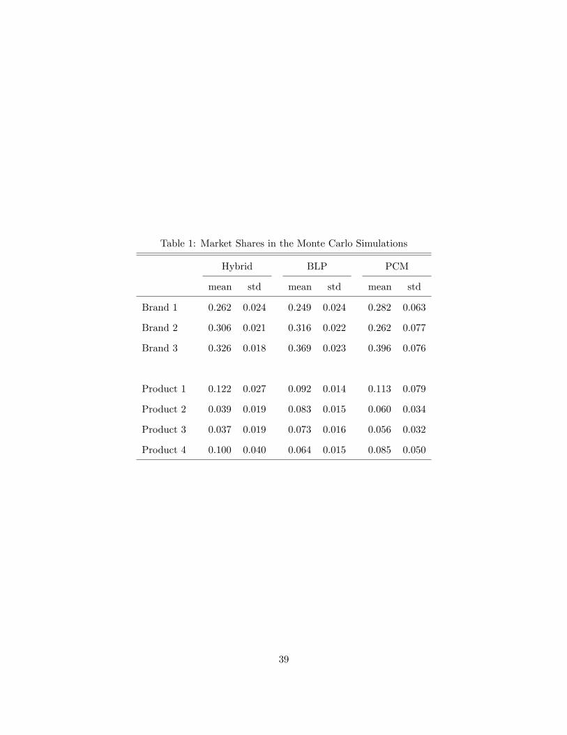
Table 1: Market Shares in the Monte Carlo Simulations

Hybrid BLP PCM

mean std mean std mean std

Brand 1 0.262 0.024 0.249 0.024 0.282 0.063

Brand 2 0.306 0.021 0.316 0.022 0.262 0.077

Brand 3 0.326 0.018 0.369 0.023 0.396 0.076

Product 1 0.122 0.027 0.092 0.014 0.113 0.079

Product 2 0.039 0.019 0.083 0.015 0.060 0.034

Product 3 0.037 0.019 0.073 0.016 0.056 0.032

Product 4 0.100 0.040 0.064 0.015 0.085 0.050

39

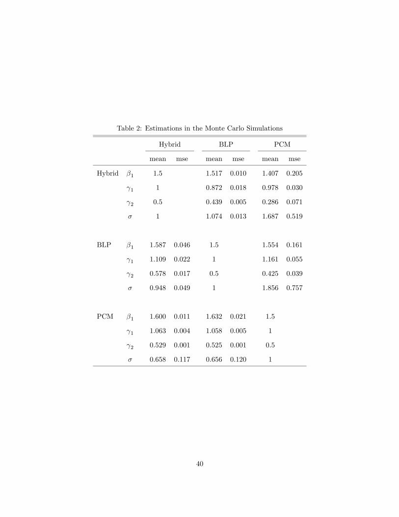
Table 2: Estimations in the Monte Carlo Simulations

Hybrid BLP PCM

mean mse mean mse mean mse

Hybrid β1 1.5 1.517 0.010 1.407 0.205

γ1 1 0.872 0.018 0.978 0.030

γ2 0.5 0.439 0.005 0.286 0.071

σ 1 1.074 0.013 1.687 0.519

BLP β1 1.587 0.046 1.5 1.554 0.161

γ1 1.109 0.022 1 1.161 0.055

γ2 0.578 0.017 0.5 0.425 0.039

σ 0.948 0.049 1 1.856 0.757

PCM β1 1.600 0.011 1.632 0.021 1.5

γ1 1.063 0.004 1.058 0.005 1

γ2 0.529 0.001 0.525 0.001 0.5

σ 0.658 0.117 0.656 0.120 1

40

Table 3: Absolute Markup in the Monte Carlo Simulations

Hybrid BLP PCM

mean std mean std mean std

Hybrid Product 1 1.075 0.279 1.116 0.281 1.234 0.556

Product 2 1.286 0.384 1.360 0.395 1.643 0.823

Product 3 1.539 0.481 1.629 0.503 2.135 1.053

Product 4 1.840 0.536 1.917 0.587 2.682 1.264

BLP Product 1 1.087 0.244 1.083 0.244 1.167 0.604

Product 2 1.301 0.364 1.337 0.406 1.658 0.942

Product 3 1.574 0.490 1.635 0.520 2.259 1.266

Product 4 1.887 0.582 1.934 0.617 2.923 1.566

PCM Product 1 0.040 0.047 0.048 0.067 0.095 0.132

Product 2 0.050 0.089 0.068 0.108 0.126 0.197

Product 3 0.098 0.171 0.114 0.181 0.207 0.327

Product 4 0.184 0.256 0.188 0.269 0.339 0.498

41

Table 4: Consumer Welfare in the Monte Carlo Simulations

Hybrid BLP PCM

mean std mean std mean std

Hybrid All Products∗ 1 1 1

No Brand 3† No Price Change 0.909 0.007 0.926 0.005 0.970 0.010

Price Change 0.875 0.013 0.906 0.013 0.961 0.025

No Product 4‡ No Price Change 0.972 0.013 0.989 0.005 0.984 0.011

Price Change 0.965 0.017 0.987 0.007 0.981 0.014

BLP All Products∗ 1 1 1

No Brand 3† No Price Change 0.915 0.008 0.930 0.004 0.982 0.007

Price Change 0.863 0.013 0.901 0.014 0.949 0.068

No Product 4‡ No Price Change 0.869 0.019 0.935 0.003 0.943 0.013

Price Change 0.839 0.023 0.923 0.005 0.923 0.025

PCM All Products∗ 1 1 1

No Brand 3† No Price Change 0.996 0.003 0.994 0.005 0.994 0.005

Price Change 0.970 0.018 0.962 0.024 0.976 0.012

No Product 4‡ No Price Change 0.984 0.012 0.991 0.006 0.980 0.017

Price Change 0.954 0.028 0.969 0.022 0.955 0.023

∗Consumer welfare with all products is normalized to 1.†All four products of Brand 3 are taken out.‡Product 4 of each brand is taken out.

42

Table 5: Trends in the Desktop Personal Computer Market from 4Q2001 to 3Q2004

Price (in dollars) Quantity (in thousands) CPU speed (in GHz)

Time mean std min max mean std min max mean std min max

4Q01 825.88 255.78 445.50 1,936.92 13.55 19.08 1.01 175.31 1.29 0.26 0.50 2.00

1Q02 827.45 259.00 350.38 2,081.72 9.51 9.90 1.03 54.09 1.35 0.26 0.60 2.20

2Q02 788.99 240.12 421.21 1,878.22 6.34 5.75 1.05 32.10 1.43 0.28 0.70 2.26

3Q02 795.12 252.50 393.65 1,987.81 6.42 6.38 1.00 29.17 1.60 0.35 0.70 2.53

4Q02 739.19 253.96 388.62 1,988.93 10.03 13.87 1.03 156.90 1.91 0.37 0.70 2.66

1Q03 718.78 291.42 360.04 2,265.47 7.15 7.43 1.00 32.67 1.97 0.36 0.70 3.06

2Q03 733.54 307.05 355.55 2,074.25 6.84 5.79 1.00 37.50 2.15 0.33 0.80 3.06

3Q03 710.00 299.60 343.41 2,073.72 7.17 9.25 1.00 57.58 2.26 0.31 1.00 3.00

4Q03 724.18 295.39 373.02 2,169.56 9.89 13.79 1.04 149.49 2.46 0.31 1.00 3.20

1Q04 729.75 289.46 322.21 2,147.68 7.15 8.49 1.01 55.13 2.55 0.33 1.00 3.20

2Q04 707.41 271.81 357.77 2,132.67 6.33 6.60 1.00 30.75 2.53 0.37 1.00 3.40

3Q04 690.64 248.03 222.14 1,699.68 7.27 7.76 1.07 44.57 2.48 0.34 1.25 3.40

43

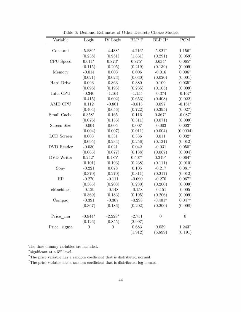
Table 6: Demand Estimates of Other Discrete Choice Models

Variable Logit IV Logit BLP I† BLP II‡ PCM

Constant -5.889∗ -4.488∗ -4.216∗ -5.821∗ 1.156∗

(0.238) (0.951) (1.831) (0.291) (0.059)CPU Speed 0.611∗ 0.873∗ 0.875∗ 0.634∗ 0.065∗

(0.115) (0.205) (0.219) (0.139) (0.009)Memory -0.014 0.003 0.006 -0.016 0.006∗

(0.021) (0.023) (0.030) (0.020) (0.001)Hard Drive 0.093 0.363 0.380 0.109 0.035∗

(0.096) (0.195) (0.235) (0.105) (0.009)Intel CPU -0.340 -1.164 -1.155 -0.374 -0.167∗

(0.415) (0.602) (0.653) (0.408) (0.022)AMD CPU 0.112 -0.801 -0.815 0.097 -0.181∗

(0.404) (0.656) (0.722) (0.395) (0.027)Small Cache 0.358∗ 0.165 0.116 0.367∗ -0.087∗

(0.076) (0.156) (0.311) (0.071) (0.009)Screen Size -0.004 0.005 0.007 -0.003 0.003∗

(0.004) (0.007) (0.011) (0.004) (0.0004)LCD Screen 0.003 0.331 0.336 0.011 0.032∗

(0.095) (0.234) (0.256) (0.131) (0.012)DVD Reader -0.030 0.021 0.042 -0.031 0.050∗

(0.065) (0.077) (0.138) (0.067) (0.004)DVD Writer 0.242∗ 0.485∗ 0.507∗ 0.249∗ 0.064∗

(0.101) (0.193) (0.238) (0.111) (0.010)Sony -0.221 0.078 0.105 -0.217 0.081∗

(0.370) (0.270) (0.311) (0.217) (0.012)HP -0.270 -0.111 -0.090 -0.270 0.067∗

(0.365) (0.203) (0.230) (0.200) (0.009)eMachines -0.129 -0.148 -0.158 -0.151 0.005

(0.369) (0.183) (0.195) (0.206) (0.009)Compaq -0.391 -0.307 -0.298 -0.401∗ 0.047∗

(0.367) (0.186) (0.202) (0.200) (0.008)

Price_mu -0.944∗ -2.228∗ -2.751 0 0(0.126) (0.855) (2.997)

Price_sigma 0 0 0.683 0.059 1.243∗

(1.912) (5.899) (0.191)

The time dummy variables are included.∗significant at a 5% level.†The price variable has a random coeffi cient that is distributed normal.‡The price variable has a random coeffi cient that is distributed log normal.

44

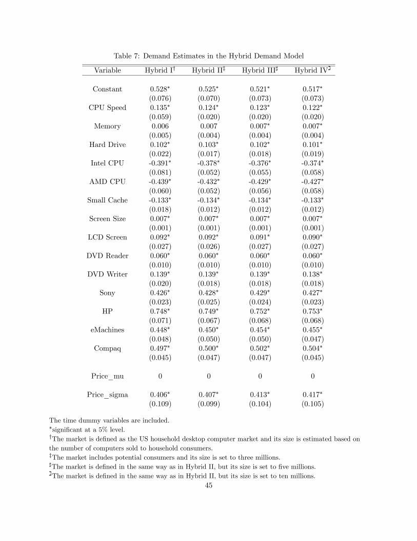
Table 7: Demand Estimates in the Hybrid Demand Model

Variable Hybrid I† Hybrid II‡ Hybrid III] Hybrid IVג

Constant 0.528∗ 0.525∗ 0.521∗ 0.517∗

(0.076) (0.070) (0.073) (0.073)CPU Speed 0.135∗ 0.124∗ 0.123∗ 0.122∗

(0.059) (0.020) (0.020) (0.020)Memory 0.006 0.007 0.007∗ 0.007∗

(0.005) (0.004) (0.004) (0.004)Hard Drive 0.102∗ 0.103∗ 0.102∗ 0.101∗

(0.022) (0.017) (0.018) (0.019)Intel CPU -0.391∗ -0.378∗ -0.376∗ -0.374∗

(0.081) (0.052) (0.055) (0.058)AMD CPU -0.439∗ -0.432∗ -0.429∗ -0.427∗

(0.060) (0.052) (0.056) (0.058)Small Cache -0.133∗ -0.134∗ -0.134∗ -0.133∗

(0.018) (0.012) (0.012) (0.012)Screen Size 0.007∗ 0.007∗ 0.007∗ 0.007∗

(0.001) (0.001) (0.001) (0.001)LCD Screen 0.092∗ 0.092∗ 0.091∗ 0.090∗

(0.027) (0.026) (0.027) (0.027)DVD Reader 0.060∗ 0.060∗ 0.060∗ 0.060∗

(0.010) (0.010) (0.010) (0.010)DVD Writer 0.139∗ 0.139∗ 0.139∗ 0.138∗

(0.020) (0.018) (0.018) (0.018)Sony 0.426∗ 0.428∗ 0.429∗ 0.427∗

(0.023) (0.025) (0.024) (0.023)HP 0.748∗ 0.749∗ 0.752∗ 0.753∗

(0.071) (0.067) (0.068) (0.068)eMachines 0.448∗ 0.450∗ 0.454∗ 0.455∗

(0.048) (0.050) (0.050) (0.047)Compaq 0.497∗ 0.500∗ 0.502∗ 0.504∗

(0.045) (0.047) (0.047) (0.045)

Price_mu 0 0 0 0

Price_sigma 0.406∗ 0.407∗ 0.413∗ 0.417∗

(0.109) (0.099) (0.104) (0.105)

The time dummy variables are included.∗significant at a 5% level.†The market is defined as the US household desktop computer market and its size is estimated based onthe number of computers sold to household consumers.‡The market includes potential consumers and its size is set to three millions.]The market is defined in the same way as in Hybrid II, but its size is set to five millions.Theג market is defined in the same way as in Hybrid II, but its size is set to ten millions.

45

Table 8: Price Elasticity in Different Demand Models

Product Elasticity Brand Elasticity

IV Logit BLP I PCM Hybrid I BLP I Hybrid I

Own elasticity -1.741 -1.882 -3,368 -1,136 -2.977 -2.355

Cross elasticity

Within-brand 4.8×10−4 4.1×10−4 1,946 489.8 n.a. n.a.

Cross-brand 4.7×10−4 3.6×10−4 1,453 0.035 0.005 0.066

% of substitutes across brands† 1 1 0.03 0.10

See Tables 6 and 7 for estimates in different demand models.The medians of each period are averaged over all periods.†The mean ratio of other brand products that are substitutes to a given brand product.

46

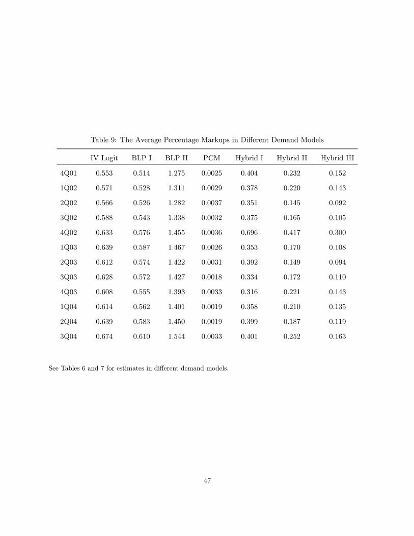
Table 9: The Average Percentage Markups in Different Demand Models

IV Logit BLP I BLP II PCM Hybrid I Hybrid II Hybrid III

4Q01 0.553 0.514 1.275 0.0025 0.404 0.232 0.152

1Q02 0.571 0.528 1.311 0.0029 0.378 0.220 0.143

2Q02 0.566 0.526 1.282 0.0037 0.351 0.145 0.092

3Q02 0.588 0.543 1.338 0.0032 0.375 0.165 0.105

4Q02 0.633 0.576 1.455 0.0036 0.696 0.417 0.300

1Q03 0.639 0.587 1.467 0.0026 0.353 0.170 0.108

2Q03 0.612 0.574 1.422 0.0031 0.392 0.149 0.094

3Q03 0.628 0.572 1.427 0.0018 0.334 0.172 0.110

4Q03 0.608 0.555 1.393 0.0033 0.316 0.221 0.143

1Q04 0.614 0.562 1.401 0.0019 0.358 0.210 0.135

2Q04 0.639 0.583 1.450 0.0019 0.399 0.187 0.119

3Q04 0.674 0.610 1.544 0.0033 0.401 0.252 0.163

See Tables 6 and 7 for estimates in different demand models.

47

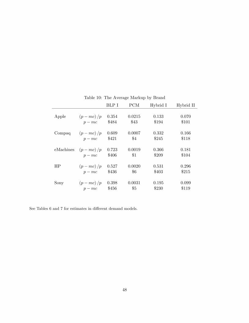
Table 10: The Average Markup by Brand

BLP I PCM Hybrid I Hybrid II

Apple (p−mc) /p 0.354 0.0215 0.133 0.070p−mc $484 $43 $194 $101

Compaq (p−mc) /p 0.609 0.0007 0.332 0.166p−mc $421 $4 $245 $118

eMachines (p−mc) /p 0.723 0.0019 0.366 0.181p−mc $406 $1 $209 $104

HP (p−mc) /p 0.527 0.0020 0.531 0.296p−mc $436 $6 $403 $215

Sony (p−mc) /p 0.398 0.0031 0.195 0.099p−mc $456 $5 $230 $119

See Tables 6 and 7 for estimates in different demand models.

48

Figure 1: The Market Share by Brand from October 2001 to September 2004

49

Figure 2: The Average Price by Brand from October 2001 to September 2004

50

Figure 3: Consumer Welfare from October 2001 to September 2004

­0.300

­0.200

­0.100

0.000

0.100

0.200

0.300

0.400

Nov­01

Jan­02

Mar­02

May­02

Jul­02

Sep­02

Nov­02

Jan­03

Mar­03

May­03

Jul­03

Sep­03

Nov­03

Jan­04

Mar­04

May­04

Jul­04

Sep­04

HybridBLPPCM

51

Figure 4: The Quality Index from October 2001 to September 2004

52

Appendix A: Data Description

Scanner data on PCs were collected from US retail outlets by NPD Techworld.24 The originaldata set contains 6,235 computer products ranging from PDAs to desktops and has 47,923 observa-tions for 36 months from October of 2001 to September of 2004. The main components of the dataset are desktop and notebook computers. There are 2,769 desktop and 2,756 notebook computerscovering 66% and 33% of the total sales respectively. The rest consists of small portable computerslike tablet PCs and subnotes. Dell’s products are not included in the data set since they are notsold at retail outlets.

IDC estimates that about 47.6 million computers were sold in the US in 2002 and 52.7million in 2003.25 And about 17.1 million were sold to household consumers in 2002 and about20 million in 2003. The total unit sold in the data set is 7.7 and 8.4 million in 2002 and 2003respectively, which means that the data set covers about 42 ∼ 45% of the US household market.Since products of Dell, which has about 30% market share in the US market, are not included, thedata set covers 60 ∼ 65% of the US retail outlet market.26

Most observations have very small sales. 53.95% of the total observations have less than10 units of sale, 78.64% less than 100 units, and 90% less than 1,000 units. However, the sale isconcentrated on a small number of products. Observations with more than 100 units cover about96% of the total sale and observations with more than 1,000 units cover about 90% of the sale.This means that 10% of observations cover 90% of the total sale. Moreover, when observations withless than 100 units are excluded, all of the outliers in price and product characteristics disappear.And the summary statistics of product characteristics do not change significantly when the cutoffis raised to 1,000 units.

Appendix B: Demand Estimation in the Random Coeffi cient Logit Model (BLP)In Table B-1 I report the IV logit estimation with different instrumental variables. The table

shows that the price coeffi cient becomes positive with the BLP-type IVs (IV 1). When productcharacteristics are interacted with the time dummy variables, the price coeffi cient becomes neg-ative. This is probably because the price does not increase over time with improving productcharacteristics. IV 4 is used to estimate BLP in Section 4.

In Tables B-2 and B-3 I report BLP estimates with different specifications. Table B-2reports variations of BLP I in Table 6. The random coeffi cients are added on the constant termand the speed variable in addition to the price variable, but they do not change estimation resultssignificantly. Table B-3 reports variations of BLP II in Table 6. Different parameters are normalizedand different instrumental variables are used for each specification.

24Aizcorbe and Pho (2005) use the same data and provide more details on the data.25Gartner estimates that 43.9 million were sold in 2002 and 57.7 million were sold in 2003.

26Gartner estimates that the market share of Dell in the US market is 29.69% in 2002 and 28.19% in 2003.

53

Table A-1: Summary Statistics of Product Characteristics

Memory (in Mega bytes) Hard Drive (in Giga bytes) Screen Size (in inches)

mean std min max mean std min max mean std min max

4Q01 232.78 131.00 64 512 42.29 18.03 20 80 16.90 0.35 15 17

1Q02 312.66 157.13 64 512 53.30 24.78 20 120 16.36 0.83 15 17

2Q02 239.29 141.12 64 512 50.36 21.28 20 120 16.50 0.84 15 17

3Q02 291.94 174.22 64 512 53.57 19.91 20 120 16.65 0.72 15 17

4Q02 306.26 157.01 128 512 63.16 23.03 20 120 16.51 0.80 15 17

1Q03 306.21 160.91 128 1024 64.83 26.45 40 250 16.27 0.96 15 18

2Q03 344.38 152.09 128 1024 74.31 30.51 40 160 16.18 0.86 15 17

3Q03 323.26 164.24 128 1024 79.17 33.01 40 160 16.45 0.89 15 17

4Q03 366.83 139.04 128 1024 88.32 39.17 40 200 16.63 0.80 15 20

1Q04 395.06 129.20 128 1024 99.97 47.95 40 250 16.68 0.82 15 20

2Q04 460.10 116.57 256 1024 111.76 52.66 40 250 16.83 0.60 15 20

3Q04 445.36 143.47 256 1024 113.17 56.84 40 250 16.90 0.47 15 19

54

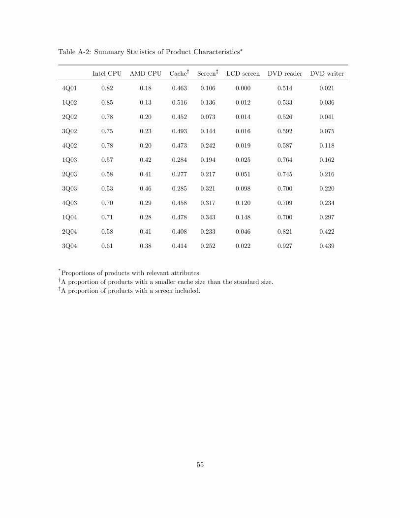
Table A-2: Summary Statistics of Product Characteristics∗

Intel CPU AMD CPU Cache† Screen‡ LCD screen DVD reader DVD writer

4Q01 0.82 0.18 0.463 0.106 0.000 0.514 0.021

1Q02 0.85 0.13 0.516 0.136 0.012 0.533 0.036

2Q02 0.78 0.20 0.452 0.073 0.014 0.526 0.041

3Q02 0.75 0.23 0.493 0.144 0.016 0.592 0.075

4Q02 0.78 0.20 0.473 0.242 0.019 0.587 0.118

1Q03 0.57 0.42 0.284 0.194 0.025 0.764 0.162

2Q03 0.58 0.41 0.277 0.217 0.051 0.745 0.216

3Q03 0.53 0.46 0.285 0.321 0.098 0.700 0.220

4Q03 0.70 0.29 0.458 0.317 0.120 0.709 0.234

1Q04 0.71 0.28 0.478 0.343 0.148 0.700 0.297

2Q04 0.58 0.41 0.408 0.233 0.046 0.821 0.422

3Q04 0.61 0.38 0.414 0.252 0.022 0.927 0.439

∗Proportions of products with relevant attributes†A proportion of products with a smaller cache size than the standard size.‡A proportion of products with a screen included.

55

Table B-1: Demand Estimates in the IV Logit Model

Variable Simple Logit IV 1† IV 2‡ IV 3♦ IV 4>

Constant -5.889∗ -9.927∗ -5.498∗ -4.722∗ -4.488∗

(0.238) (1.711) (0.735) (0.916) (0.951)CPU Speed 0.611∗ -0.115 0.565∗ 0.828∗ 0.873∗

(0.115) (0.342) (0.162) (0.198) (0.205)Memory -0.014 -0.069 -0.005 -0.001 0.003

(0.021) (0.037) (0.022) (0.023) (0.023)Hard Drive 0.093 -0.658 0.149 0.318 0.363

(0.096) (0.338) (0.157) (0.189) (0.195)Intel CPU -0.340 1.973 -0.446 -1.016 -1.164

(0.415) (1.049) (0.469) (0.582) (0.602)AMD CPU 0.112 2.721 -0.058 -0.637 -0.801

(0.404) (1.155) (0.504) (0.633) (0.656)Small Cache 0.358∗ 0.953∗ 0.310∗ 0.199 0.165

(0.076) (0.268) (0.128) (0.151) (0.156)Screen Size -0.004 -0.030∗ -0.004 0.004 0.005

(0.004) (0.012) (0.006) (0.007) (0.007)LCD Screen 0.003 -0.941∗ 0.102 0.277 0.331

(0.095) (0.415) (0.187) (0.227) (0.234)DVD Reader -0.030 -0.191 -0.010 0.014 0.021

(0.065) (0.102) (0.070) (0.076) (0.077)DVD Writer 0.242∗ -0.491 0.325∗ 0.446∗ 0.485∗

(0.101) (0.328) (0.158) (0.188) (0.193)Price -0.944∗ 2.759 -1.245 -2.012∗ -2.228∗

(0.126) (1.575) (0.656) (0.824) (0.855)Validity of IVs Yes Yes Yes Yes

†IV 1: BLP IVs. Characteristics used are CPU Speed, Memory, Hard Drive, Screen Size, and DVD

Writer‡IV 2: CPU Speed variable interacted with time dummy variables♦IV 3: BLP IVs interacted with time dummy variables>IV 4: BLP IVs interacted with time dummy variables excluding Hard Drive and DVD Writer variables.All specifications include dummy variables for firm and time.

56

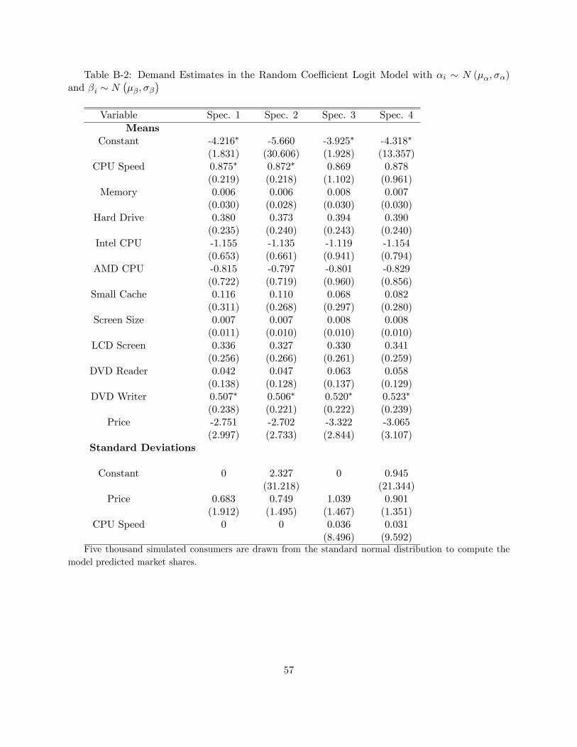
Table B-2: Demand Estimates in the Random Coeffi cient Logit Model with αi ∼ N (µα, σα)and βi ∼ N

(µβ, σβ

)Variable Spec. 1 Spec. 2 Spec. 3 Spec. 4

MeansConstant -4.216∗ -5.660 -3.925∗ -4.318∗

(1.831) (30.606) (1.928) (13.357)CPU Speed 0.875∗ 0.872∗ 0.869 0.878

(0.219) (0.218) (1.102) (0.961)Memory 0.006 0.006 0.008 0.007

(0.030) (0.028) (0.030) (0.030)Hard Drive 0.380 0.373 0.394 0.390

(0.235) (0.240) (0.243) (0.240)Intel CPU -1.155 -1.135 -1.119 -1.154

(0.653) (0.661) (0.941) (0.794)AMD CPU -0.815 -0.797 -0.801 -0.829

(0.722) (0.719) (0.960) (0.856)Small Cache 0.116 0.110 0.068 0.082

(0.311) (0.268) (0.297) (0.280)Screen Size 0.007 0.007 0.008 0.008

(0.011) (0.010) (0.010) (0.010)LCD Screen 0.336 0.327 0.330 0.341

(0.256) (0.266) (0.261) (0.259)DVD Reader 0.042 0.047 0.063 0.058

(0.138) (0.128) (0.137) (0.129)DVD Writer 0.507∗ 0.506∗ 0.520∗ 0.523∗

(0.238) (0.221) (0.222) (0.239)Price -2.751 -2.702 -3.322 -3.065

(2.997) (2.733) (2.844) (3.107)Standard Deviations

Constant 0 2.327 0 0.945(31.218) (21.344)

Price 0.683 0.749 1.039 0.901(1.912) (1.495) (1.467) (1.351)

CPU Speed 0 0 0.036 0.031(8.496) (9.592)

Five thousand simulated consumers are drawn from the standard normal distribution to compute themodel predicted market shares.

57

Table B-3: Demand Estimates in the Random Coeffi cient Logit Model with log (αi) ∼ N (µ, σ)

Variable IV 2† IV 4‡

Spec. 1 Spec. 2 Spec. 1 Spec. 2

Constant -5.772∗ -6.501∗ -5.821∗ -2.855(0.226) (1.160) (0.291) (1.900)

CPU Speed 0.508∗ 0.385∗ 0.634∗ 0.825∗

(0.150) (0.178) (0.139) (0.207)Memory -0.009 -0.018 -0.016 0.011

(0.020) (0.025) (0.020) (0.028)Hard Drive 0.089 -0.051 0.109 0.365

(0.126) (0.184) (0.105) (0.217)Intel CPU -0.262 0.130 -0.374 -1.002

(0.437) (0.523) (0.408) (0.621)AMD CPU 0.149 0.599 0.097 -0.673

(0.436) (0.579) (0.395) (0.693)Small Cache 0.352∗ 0.462∗ 0.367∗ 0.051

(0.073) (0.173) (0.071) (0.226)Screen Size -0.006 -0.011 -0.003 0.008

(0.004) (0.007) (0.004) (0.009)LCD Screen 0.015 -0.154 0.011 0.275

(0.163) (0.212) (0.131) (0.234)DVD Reader -0.019 -0.042 -0.031 0.089

(0.068) (0.081) (0.067) (0.102)DVD Writer 0.262∗ 0.136 0.249∗ 0.508∗

(0.121) (0.190) (0.111) (0.218)

Price (µ) 0 -1.422 0 2.115∗

(3.949) (0.744)Price (σ) 0.381 1 0.059 1

(1.456) (5.899)

Two thousand simulated consumers are drawn from the standard normal distribution to compute themodel predicted market shares.

†CPU Speed is interacted with time dummy variables.‡BLP IVs are interacted with time dummy variables.

58