A History of Radar Meteorology:

People, Technology, and Theory

Jeff Duda

Overview

• Will cover the period from just before World

War II through about 1980

– Pre-WWII

– WWII

– 1940s post-WWII

– 1950s

– 1960s

– 1970s

2

3

Pre-World War II

• Concept of using radio waves established starting in the very

early 1900s (Tesla)

• U.S. Navy (among others) tried using CW radio waves as a

“trip beam” to detect presence of ships

• First measurements of ionosphere height made in 1924 and

1925– E. V. Appleton and M. A. F. Barnett of Britain on 11 December 1924

– Merle A. Tuve (Johns Hopkins) and Gregory Breit (Carnegie Inst.) in July 1925• First that used pulsed energy instead of CW

4

Pre-World War II

• Robert Alexander Watson Watt

• “Death Ray” against Germans

• Assignment given to Arnold F.

“Skip” Wilkins:– “Please calculate the amount of radio

frequency power which should be radiated

to raise the temperature of eight pints of

water from 98°F to 105°F at a distance of 5

km and a height of 1 km.”

– Not feasible with current power production

Watson Watt

5

Pre-World War II

• Watson Watt and Wilkins pondered whether radio waves could

be used merely to detect aircraft

• Memo drafted by Watson Watt on February 12, 1935:

“Detection of Aircraft by Radio Methods”– Memo earned Watson Watt the title of “the father of radar”

– Term “RADAR” officially coined as an acronym by U.S. Navy Lt. Cmdr.

Samuel M. Tucker and F. R. Furth in November 1940

• The Daventry experiment– February 26, 1935

– First recorded detection of aircraft by radio waves

– Began the full-speed-ahead development of radar for use in the coming war

6

Pre-World War II• Orford village

– First site for radar development (spring

1935)

– Watson Watt recruited Welsh physicist

Eddie Bowen among three others to

develop radar

– Slowly but surely improved the

technology• Reduced wavelength and maximum range

from hundreds of meters and units of miles to

under 1 m and up to 100 miles within one year

• Bawdsey Manor (mid-1936)– More “official” (main lab) first site for

research and development

– Development of the Chain Home

defense system

– Bowen: “get these things into fighter

planes!”7

World War II

• Big development: cavity magnetron– Capable of increasing power output tenfold

plus• 30 – 40 W → 400 W at ~10 cm

– Invented by John Randall and Henry Boot at

the University of Birmingham on February

21, 1940

– Opened the door wide for significant

development

8

World War II

• Problem: British taking a lot of abuse from German Luftwaffe

bombing missions, can’t develop the technology on their own

• Solution: ask the Americans for help

• The Tizard Mission (August – October 1940)– Aka, “The British Technical and Scientific Mission to the United States”

– Secret mission across the Atlantic on the Duchess of Richmond to Nova Scotia

first

– Eddie Bowen among the leaders

– British hoped to trade one secret for another, but after being unable to reach an

agreement with the Americans, Churchill was okay with just sharing the secret

for free

– First tests showed the cavity magnetron could output 10 – 15 kW at ~10 cm!

9

World War II

• With help from Alfred Loomis and Vannevar Bush, funding for

full-scale development in America began in October 1940– Initial budget for first year: $455,000

– After much argument, location was chosen: MIT• Secrecy (who would suspect something so significant being developed at a university?)

• Initially named Microwave Laboratory → Radiation Laboratory to allay suspicion (common

practice for the development of radar during the war)

– Some initial scientists/researchers: Eddie “Taffy” Bowen,

Ernest O. Lawrence, Isidor Isaac Rabi, Lee A. Dubridge

(oversaw the “Rad Lab” for the first few years)

– “The” place to be for radar development in America during

the war

Alfred Loomis10

World War II

• Radar continues to be developed slowly but surely, now

mainly at the Rad Lab and Telecommunications Research

Establishment

• Radar gave Allied powers big advantage– U-boats: sneaky “b---ards” hung out along the east coast of N. America and

west coast of Europe, frequently sinking battleships, destroyers, and carriers

– After Air-to-Sea-Vessel (ASV) detection developed and put into airborne

fighters, one-third of all U-boats shot down between March-June 1943

– Unfortunately, a Pathfinder (bomber) carrying the radar technology was shot

down over Holland on 2 February 1943; the Germans reverse engineered the

technology; almost overnight, all German U-boats, as well as other vehicles,

had microwave detecting technology• The Rotterdam-Gerät

– Centimeter radar was considered the technology that gave the Allies the edge in

winning the Battle of the Atlantic, and arguably, the war11

Weather Radar during WWII• Not much to say (not a priority)

• First detection of precipitation echoes likely in England in late

1940– First detection at Rad Lab: 7 February 1941

• Precipitation echoes regarded as nuisance or “clutter”,

undesirable, throughout the war

• Most radars X-band (3 cm wavelength) or S-band (10 cm

wavelength)– Letter codes for bands used for secrecy

• First U.S. publication regarding meteorological weather

echoes: “Radar echoes from atmospheric phenomena” (Bent,

1943)– Covered observations made between March 1942 and January 1943

– Erroneously explained the bright band; hadn’t seen work of the Rydes yet 12

1940s post-WWII

• Secrecy no longer important

• Weather Radar Research Project at MIT: 15

February 1946– Initial project director: Alan Bemis

• U.S. Air Force All Weather Flying Division: project

AW-MET-8 formed in December 1945

– David Atlas among the first to lead

• Project Stormy Weather in Canada: 1943

– AKA the “Stormy Weather Group” after 1950 at McGill

University

– First led by J. Stewart Marshall

Alan Bemis

Dave Atlas13

1940s post-WWII

• John Walter Ryde (and wife Dorothy)– Ryde (1941); Ryde and Ryde (1944); Ryde

(1946)

– Developed the theory of scattering and

attenuation of microwaves• “The attenuation and radar echoes produced at

centimetre wavelengths by various meteorological

phenomena”; not published until after WWII

• Computed backscatter cross sections by hand

• Used the works of Rayleigh (1871), Mie (1908), and

Gans (1912)

• Years ahead of their time; disbelieved or ignored by

peers for awhile

– Also computed early Z-R relationships using

DSDs from Lenard (1904), Humphreys (1929),

and Laws and Parsons (1943)

14

1940s post-WWII

• J. Stewart Marshall– Met Walter Palmer while working in

Ottawa

• Stormy Weather Group focused on

precipitation and cloud microphysics

• Investigation of Z – R relationships

– Wexler and Swingle (1947): “Radar storm

detection”

– Marshall et al. (1947): “Measurement of

rainfall by radar”

– Marshall and Palmer (1948): “The

distribution of raindrops with size”

• Marshall and Palmer (1948) seminal

work in the field

15

1940s post-WWII

• More on Marshall-Palmer distribution and Z – R relationships– Z = 200*R1.6 (Marshall and Palmer 1948)

– “It may be possible therefore to determine with useful accuracy the intensity of

rainfall at a point quite distant (say 100 km) by the radar echo from that point.”

– Many other researchers suspicious of their computations due to simplicity

– Other papers like Twomey (1953), Imai et al. (1955), Atlas and Chmela (1957),

and Fujiwara (1960, 1965) derived other relationships in which reflectivity for

a given rain rate differed by up to 38%, but they also remarked that there were

physical explanations for the differences; could choose a relationship based on

physical explanation and for a particular situation

16

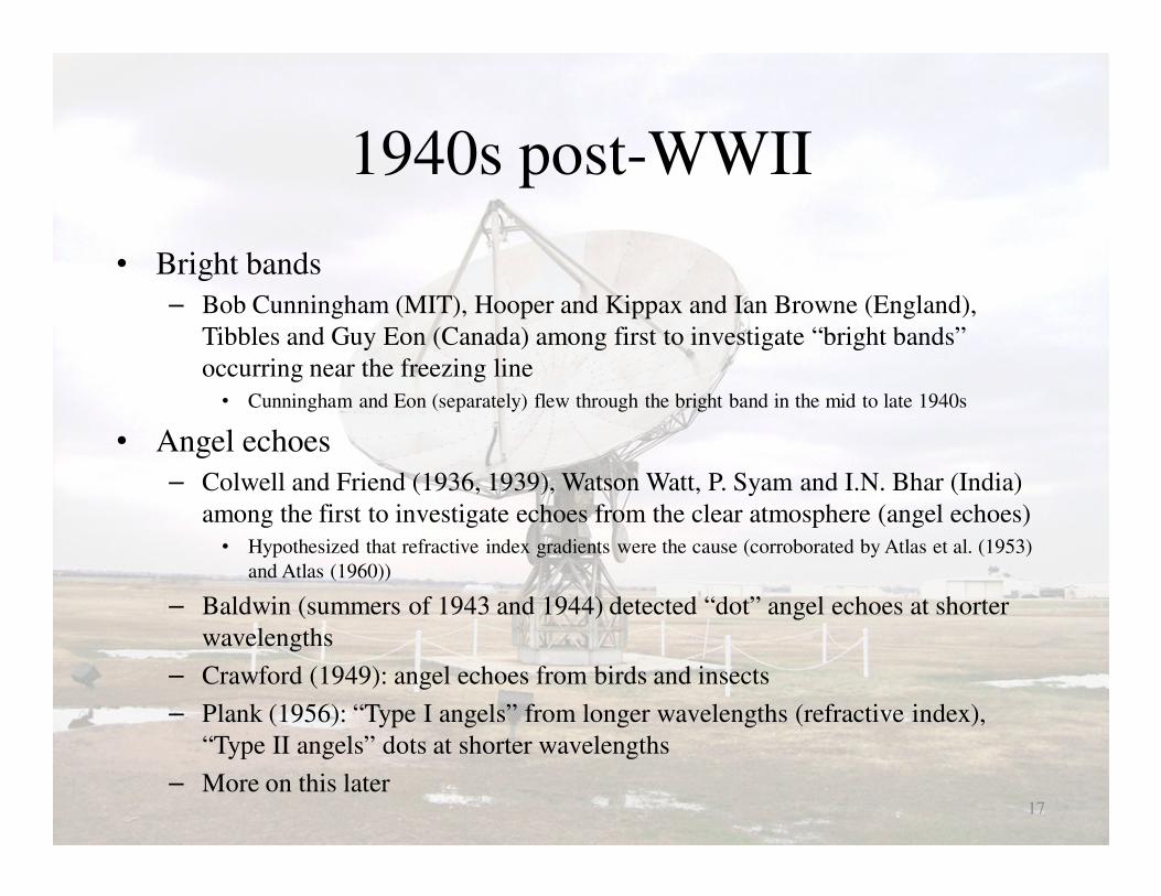
1940s post-WWII

• Bright bands

– Bob Cunningham (MIT), Hooper and Kippax and Ian Browne (England),

Tibbles and Guy Eon (Canada) among first to investigate “bright bands”

occurring near the freezing line• Cunningham and Eon (separately) flew through the bright band in the mid to late 1940s

• Angel echoes

– Colwell and Friend (1936, 1939), Watson Watt, P. Syam and I.N. Bhar (India)

among the first to investigate echoes from the clear atmosphere (angel echoes)• Hypothesized that refractive index gradients were the cause (corroborated by Atlas et al. (1953)

and Atlas (1960))

– Baldwin (summers of 1943 and 1944) detected “dot” angel echoes at shorter

wavelengths

– Crawford (1949): angel echoes from birds and insects

– Plank (1956): “Type I angels” from longer wavelengths (refractive index),

“Type II angels” dots at shorter wavelengths

– More on this later17

Bright bands and angel echoes

18

1940s post-WWII

• AN/CPS-9: first radar designed specifically for meteorological use

• Thunderstorm Project (Florida and Ohio, 1946 and 1947)– First multiagency field experiment for thunderstorm study and that relied so heavily

on radar for research

• Iso-echo contouring technique developed by Atlas, 1947

– Suppresses higher reflectivity values making gradients easier to see

• 14 March 1947: first Weather Radar Conference held at MIT

– Over 90 attendees from various agencies

• Operational radar meteorology forming

– Weather Bureau obtained 25 AN/APS-2 radars, modified them, and renamed them

WSR-1s, 1As, 3s, and 4s• First was commissioned at Washington D.C. on 12 March 1947

• Part of the Basic Weather Radar Network, established in 1946

19

1940s post-WWIIother notes

• Shipley (1941) uses the word “cell” to relate lightning

activity from thunderstorms

• Workman and Reynolds (1949) thought “cells” on radar

might actually represent fundamental units of

electrification and precipitation in thunderstorms

20

1950s

• Improving technology– Pulse integrator

• Used to get quantitative reflectivity measurements

– Sweep integrator• Developed by Nobuhiko Kodaira of Japan

• Enabled display of signals in 2D and 13 intensity levels

– R-meter• Developed by Walter Rutkowski

• Measures spectral width of a signal

• Rod R. Rogers used R-meter to try to separate components of spectrum width, unsuccessful

– CAPPI (constant altitude plan position indicator)• PPI was in use during WWII

– FASE (fast azimuth slow elevation)• Scanning strategy improved display of radar data

21

1950s

• U.S. operational radar networks underway– 1954 & 1955: several hurricanes struck the U.S. Atlantic coast

• No radar to detect them

– Weather Bureau appeals to Congress and gets funded in 1956, buys 31 radars

which will become WSR-57s• Built by Raytheon

• Had radomes (most previous radars didn’t, none of

previous operational radars did)

• 14 placed ~200 nmi apart along the coast

• First operational WSR-57 installed in Miami in June 1959

• 11 placed in the Midwest for storm detection

• Network will continue to expand through the 1960s

WSR-57 console

22

1950sAdvances in meteorology due to radar

• “Mesoscale” meteorology

– Myron Ligda, 1951: many

meteorological echoes of a size

not observed before (between

synoptic and storm/micro scale);

I’ll call them “mesoscale”

• Mesoscale meteorology would

not exist today if it weren’t for

radar!Excerpt from Radar in Meteorology,

Chapter 13, page 107

23

1950sMore advances

• Investigation of polarization diversity– Reginald Newell, Spiros Geotis, and Aaron Fleisher (MIT) studied variable

polarization of a 3-cm radar• Investigated measurement of orientation and shape of falling particles using both linearly and

circularly polarized waves

– Atlas et al. (1953) used circular and linear depolarization ratios to distinguish

hydrometeor shapes

– Early thoughts: falling hailstones had a horizontal orientation like raindrops,

and thus indistinguishable

– Research of polarization diversity dwindled during the 1960s, so little work

was done on this after the 1950s; it picked back up starting in the late 1960s,

though

24

1950sMore advances

• Stormy Weather Group investigates hail (Alberta Hail Studies

Project – ALHAS)– Designed to stop hail from falling to protect farmers from losing their crops

– Spotter network of farmers reported hail

– Decca type-41 storm radar pointed vertically to measure hail

– Never able to stop hail operationally (some experimentation was loosely

successful), but discovered many interesting facts relating probability of hail to

cloud top height: cloud tops that penetrated the tropopause much more likely to

produce large hail

– Results of this study agreed with those from similar studies in New England

and Texas with differences in actual range of cloud top height for hail

occurrence

– Variable polarization data from this study showed hailstones to have a random

orientation

25

1950sMore advances

• Storm detection and measurement– First hook echo discovery on a tornadic storm on 9

April 1953 in Illinois

– Garrett and Tice (1957) and Bigler (1958) identified

BWERs in tornadic storms

– Nolen (1959) found that ¾ of tornadoes studied

formed within a reflectivity pattern with a wave in a

line and called it a line-echo wave pattern (LEWP)

– Wokingham, England storm of 9 July 1959 passed

very close to the radar in southeast England• New observations obtained – storm did not change cloud top

height or mass character for one hour, echo-free vault region

(Keith Browning)

• Last storm to pass through southeast England for years

– 11 September 1954: Hurricane Edna observed by

multiple radars• FPS-4 (3 cm) first to get a vertical cross section through the eye

of a hurricane 26

1950sMore advances

• Advent of Doppler radar– Ian Browne and Peter Barratt (Cambridge) first to demonstrate the use of Doppler

techniques to calculate motion• 27 May 1953: vertical motion measured in a rain shower

– Doppler spectrum consistent with 2 m/s downdraft

– Paper reporting this (Barrat and Browne, 1953) not published or publicized at conferences for a few years

– James Brantley and Barczys got that work published and presented• Brantley and Barczys (1957): CW Doppler measurements of

weather echoes

– Brantley convinced Vaughn Rockney that this could

be used for tornado detection; applied for grant• 92 m/s winds measured by radar in tornado in El Dorado, KS

on 10 June 1958

– Thus began the Doppler era

27

1950s

• Texas Tornado Warning Network– Kicked off on 24 June 1953, but took 6 years to bring the network up to full

strength, at which time 17 radars were in use

– Volunteer spotter networks

– Used modified APS-2F (WSR-1,-1A,-3,-4)

– Texas A&M University managed the funds and arranged for the modifications

• 5 April 1956: Bryan and College Station, TX tornado

– Tornadic “hook” signature detected by APS-2F radar at Texas A&M Univ. at

2:00 PM• Ironically, not part of the Texas Tornado Warning Network

– At 2:45 PM, Texas A&M meteorologists told Bryan PD that tornado would

touch down in 30 minutes• Actual damage started at 3:09 PM

• Bigler (1956): A note on the successful identification and tracking of a tornado by

radar. Weatherwise

28

1950sOther notes

• 3rd Conference on Radar Meteorology held at McGill University in

1952

– First suggestion of using “preprints” made by Marshall

• 6th Conference on Radar Meteorology held at MIT in March 1957

– “More data!” they wanted

• Radar Meteorology, 1959, Louis Battan

– First textbook on radar meteorology

– Translated into Chinese for use by students and meteorologists in China until they

were able to obtain their own research radars in the 1960s

• Bergeron process becomes better defined and better understood

– 1930s: ice crystals grow at expense of liquid water

– 1940s: observations show rain from clouds not exceeding the freezing level• Coalescence process for precipitation growth first suggested

– 1950s: agreement that Bergeron process and coalescence compete for precip growth

29

“More Data!”

Louis Battan

30

1960s• Further improving technology

– Sweep generator modified (Donat Hoegl) to get more pulses to measure a volume (1962)• Effectively increased the resolution of radar images

• Mario Schaffner digitized sweep integrator in 1966

– Storm Radar Data Processor – (1960) – David Atlas• Enabled processing and displaying of radar data in real time; digital display

• Beginnings of digital radar meteorology in the 1960s

– RAYSPAN frequency analyzer• Used to construct the first vertical wind profile using the Velocity-Azimuth Display technique (27 May 1961)

– Coherent Memory Filter → Plan Shear Indicator• Developed by Graham Armstrong in 1966

• Used to display Doppler velocity data on a PPI

– Calibrated Echo Intensity Control (CEICON), 1966• Enabled control of reflectivity levels by inserting various degrees of attenuation into radar software

– Video Integrator and Processor, 1968• Allowed radar to average instantaneous backscattered power from targets, thus automating and standardizing

measurements

• Allowed display of six values of reflectivity based on rain rates

31

1960s

• Radar equation updated– Initial work by Rydes assumed target was small compared to radar volume

(single targets like planes)

– Meteorological targets fill volume

– Result: much higher predicted values of reflectivity compared to experimental

values obtained

32

1960s

• More advances in storm detection and structure– Walter Hitschfield discovers splitting storms in 1960; splitting storms further

investigated by Browning, Donaldson, and Hammond• Tornadic storm near Wichita Falls, TX on 4 April 1964 observed by NSSL radar to move to the

left of, and faster than, the mean wind vector! Another one seen on 23 April!

• Storm relative winds for right and left movers formed a mirror image

– Geary, OK storm of 1961 well documented to have weak echo regions• First to be identified as a supercell

– Donaldson (1961): different types of storms have different vertical profiles of

reflectivity• Only rain: decreasing reflectivity with height

• Tornadic: pronounced maximum aloft, decreasing from there

– First detection of mesocyclone on radar using PSI by Donaldson on 9 August

1968

33

34

1960s

• Further development of Doppler radar– Atlas (1963) suggested playing with PRF to be able to measure high velocities

(requires high PRF) and measure echoes at distant ranges (requires low PRF)• “Doppler dilemma”, problem had been recognized in the late 1950s; technology was lagging

substantially behind theory and practice

– Dual-Doppler wind measurements• First made on 2 May 1967 in a rain shower in England (Peace and Brown, 1968)

• Used one radar pointing vertically and another displaced horizontally looking horizontally into

the same area

– Rummler (1968) developed the pulse pair technique to obtain mean and

variance computations of Doppler velocities• First applied in 1972

35

1960s

• More research on clear air echoes– Wallops Island, VA research (Atlas)

• Started in 1964

• First observation of tropopause on radar

• Battan (1973) concluded that clear air echoes at wavelengths of 3 cm or less due to insects or

birds and those at 10 cm or longer due to refractive index fluxuations (not necessarily tight

gradients)

– Hardy and Ottersten (1969) showed donut

shaped clear air echoes due to boundaries of

dry convective thermals

36

1960s

• Operational networks expanding– Air Weather Service replaces FPS-68 with FPS-77 radar

• C-band to compromise between X and S bands

• First installed in March 1966; most installed by 1969

• Poor/no training, maintenance early on

– 14 more WSR-57s obtained by Weather Bureau in

1966-1967 to fill holes in coverage east of the Rockies• Up to 1966 all radars located near Weather Bureau/NWS offices; some of the new 14 weren’t;

were placed in places to optimize coverage

FPS-77 console

37

1970s

• Technology improvements– Movement of radar systems to computer based; digitizing

• Increased storage capacity dramatically from magnetic tape method

– Color radar displays• First invented by Ken Glover of Air Force Geophysics Lab and colleagues at Raytheon in 1974

– VIL technique invented by Greene and Clark (1971)

– Display techniques• HARPI, PPHI, AZLOR, ADA

38

1970s

• Storm detection using Doppler radar– Michael Krauss first unequivocal observation of a tornado on radar on 9

August 1972 (Brookline, MA)• “unequivocal” because it was sighted by NWS employees and an MIT student at the same time

it was being observed on radar

– Union City, OK tornado of 24 May 1973 observed by chasers and radar• Close enough to radar site to resolve what would later be called a “tornado vortex signature” by

Brown and Lemon (1976)

• Dual-Doppler radar network established

– One at NSSL in 1971, the other at Cimarron Field, OK in 1973

39

1970sOperational networks upgrading

• Enterprise Electronics Corporation developed a new brand of S- and

C-band radars

– First went to a TV station in Tampa, FL in 1969 (WSR-74S)

– NWS got funded to buy 66 in 1976 to replace aging WSR-57s; called them

WSR-74Cs

• Would buy 16 more between 1981 and 1985 – the last purchase made before

NEXRAD

• Some WSR-57s survived until upgraded to WSR-88Ds

• NWS conducted D/RADEX from 1971 – 1976

– Tested digitizing of radar output for meteorology and hydrology

– 5 WSR-57s used

– Idea tested: gradually increase antenna tilt to get a volume scan

40

1970sOperational networks upgrading

• Joint Doppler Operational Project (JDOP): 1977 – 1979– Battan (1976) and Atlas (1976) wrote reviews on Doppler radar to present to U.S.

government

– NWS and NSSL declare plans to upgrade operational network to Doppler capability

with or without DOD

– As much an operational experiment as it was a research experiment

– Success led immediately to the creation of the NEXRAD network

• Severe Environmental Storms and Mesoscale Experiment (Project

SESAME): spring 1979

– Conducted in the southern plains states

– Data aided JDOP• 10 April 1979 Witchita Falls, TX tornado invisible to a 5-cm radar due to attenuation, but plainly

visible to a 10-cm radar in a similar position

• Convinced project investigators to use 10-cm radar instead of 5-cm radar

• Successful studies of clear-air echoes in the 1970s led to the requirement

that NEXRAD radars be capable of detecting these echoes, especially in

the boundary layer and also being able to obtain Doppler velocities 41

1970s

• More studies of clear air echoes– Browning et al. (1972, 1973) studied Kelvin-Helmholtz waves in atmosphere

• Ben Balsley, Warner Ecklund, and David Carter (NOAA Aeronomy

Lab) showed use of VHF/UHF radars to determine atmospheric

winds

– Ecklund et al. (1979) used Platteville, CO radar to measure winds in 1978

– Work like this led to the establishment of the Colorado Wind Profiling

Network, and then the NOAA Profiler Network 42

NOAA Profiler Network

43

NEXRAD Network today

44

45

Atlas, D., and Coauthors, 1990: Radar in Meteorology. Amer. Meteor. Soc., 806 pp.

Buderi, R., 1996: The Invention that Changed the World. Simon and Schuster, 575 pp.

Doviak, R. J., and D. S. Zrnić, 1993: Doppler Radar and Weather Observations. 2nd Ed.,

Academic Press, 562 pp.

Probert-Jones, J. R., 1962: The radar equation in meteorology. 551.501.Sl : 551.508.S5 :

621.396.91

Whiddington, R., 1962: John Walter Ryde. 1898 – 1961. Bio. Mem. Fellows Roy. Soc., 8,

105 –117.

Whiton, R. C., P. L. Smith, S. G. Bigler, K. E. Wilk, and A. C. Harbuck, 1998a: History of

operational use of weather radar by U.S. weather services, Part I: The pre-NEXRAD

era. Wea. Forecasting, 13, 219 – 243.

―, ―, ―, ―, 1998b: History of operational use of weather radar by U.S. weather services, Part

II: Development of operational Doppler weather radars. Wea. Forecasting, 13, 244 –

252.

References

46