A hierarchical approach to construct Petri nets for

A hierarchical approach to construct Petri nets for modeling the faultpropagation mechanisms in sequential operations

Yi-Feng Wang, Chuei-Tin Chang *

Department of Chemical Engineering, National Cheng Kung University, Tainan 70101, Taiwan, ROC

Received 18 March 2002; received in revised form 5 September 2002; accepted 5 September 2002

Abstract

A systematic procedure has been proposed to construct Petri nets for modeling the fault propagation behaviors in batch processes.

In this work, a complete system model is organized according to a hierarchy of four levels, i.e. (1) the controller/operator; (2) the

valves; (3) the process units; and (4) the sensors. Every component in this system model consists of two distinct elements. One is used

to characterize the equipment states and the other the input�/output relations. For the purpose of reducing model construction

effort, the general structure of object-oriented abbreviations is also developed to represent the PN in a user-friendly format. The

effectiveness and correctness of this approach have been successfully demonstrated with a number of practical examples.

# 2002 Elsevier Science Ltd. All rights reserved.

Keywords: Sequential operation; Petri net; Digraph; Hazard analysis; Fault propagation mechanism; Hierarchical approach

1. Introduction

In order to ensure operation safety, hazard analysis is

one of the basic tasks that must be performed in

designing or revamping any chemical process. Numer-

ous techniques are available for this purpose, e.g. fault

tree analysis (FTA), event tree analysis (ETA), failure

modes and effects analysis (FMEA) and hazard and

operability study (HAZOP), etc. In implementing these

methods, there are always needs (1) to reason deduc-

tively for finding all combinations of basic events that

could lead to an undesirable condition and/or (2) to

predict all possible consequences of a given fault origin.

However, if every fault propagation mechanism is to be

identified manually, a rigorous hazard analysis is bound

to be labor- and time-consuming and its results often

error-prone. To alleviate these practical problems, there

have been many attempts in the past to develop

computer aids on the basis of various qualitative

models.

In the last two decades, the research on automatic

hazard analysis has advanced significantly. Many effi-

cient tools have been adopted to develop the fault-tree

synthesis algorithms, e.g. digraph (Lapp & Powers,

1977; Chang & Hwang, 1992), decision table (Kuma-

moto & Henley, 1979) and mini-fault tree (Kelly & Lees,

1986a,b). Several generic expert systems have also been

constructed to produce comprehensive HAZOP reports

(Vaidhyanathan & Venkatasubramanian, 1996a,b). The

prerequisite for identifying the fault propagation me-

chanisms in implementing any of these methods is

basically a qualitative system model. It can be observed

from the literature that the digraph is by far the most

popular choice (Allen & Rao, 1980; Andrews &

Morgan, 1986; Chang & Hwang, 1994; Chang, Hsu &

Hwang, 1994). Although the digraph-based approach

has been proven to be useful, it is effective mostly in

applications concerning the continuous processes. This

is due to the fact that the digraph is inherently

unsuitable for describing the dynamic causal relation-

ships among time, discrete events, equipment states and

system configurations in the batch or semi-batch pro-

cesses.

In this work, the Petri net (PN) is used as a modeling

tool to circumvent the above drawbacks. The ordinary

Petri net (Petri, 1962) is well known for its capability in

describing the discrete-event systems. However, it is also

apparent that this original version of PN lacks the* Corresponding author. Fax: �/886-6-234-4496

E-mail address: [email protected] (C.-T. Chang).

Computers and Chemical Engineering 27 (2003) 259�/280

www.elsevier.com/locate/compchemeng

0098-1354/02/$ - see front matter # 2002 Elsevier Science Ltd. All rights reserved.

PII: S 0 0 9 8 - 1 3 5 4 ( 0 2 ) 0 0 1 9 3 - X

mailto:[email protected]

capability of representing the relationships among con-tinuous process variables. Consequently, the idea of

automating procedure HAZOP on the basis of Petri

net�/digraph hybrid models was proposed in recent

literature (Srinivasan & Venkatasubramanian,

1998a,b). From a critical review of these works, one

can observe that this modeling approach is not suitable

for depicting a number of important features in more

complex batch (sequential) operations. Specifically,

1.1. Concurrent activities

Concurrent activities can be easily expressed in terms

of Petri nets. Most batch chemical processes are

designed with a certain degree of parallelism to ensure

flexibility and efficiency in operation. This type of

operation has not been considered in the publishedstudies.

1.2. Cyclic operations

In a sense, all batch operations are repetitive or cyclic.

It is thus necessary to investigate the possibilities of a

current failure causing undesirable consequences in the

later cycles. Therefore, in certain cases, it is not enoughto build a recipe-based PN model representing the

operation steps only in a single batch (or cycle).

1.3. Continuous transients

The batch operations are typically characterized by

time-variant operating conditions and/or process vari-

ables. These quantities were discretized and expressedwith digraphs in the hybrid models proposed by

Srinivasan and Venkatasubramanian (1998a,b). How-

ever, since these transients can be better described with

the continuous places, there is a strong incentive to

model the batch systems in a unified format with PNs

only.

1.4. Multi-purpose productions

It is a common practice to manufacture more than

one product with the same facilities in a batch plant.

Due to the need to share resources, it may be necessary

to run some units under different operation modes at

different times. As a result, the process configuration,

i.e. the connections among units, may be changed

accordingly. Since the conventional recipe-based PN

models are built individually for a single product, they

cannot be easily integrated to represent the overall

orchestrated production activities efficiently.

It should be noted that a large number of enhance-

ments have already been introduced since the original

PN was proposed (Peterson, 1981; David & Alla, 1994;

Alla & David, 1998). Two commonly used versions, i.e.

extensions and abbreviations , can be found in the

literature. The extensions are used to enrich the ordinary

PN by incorporating additional functions and thereby

allow a greater number of applications to be treated.

For example, David (1997) developed the hybrid and

continuous Petri nets to model a number of realistic

engineering systems. On the other hand, the abbrevia-

tions are used to simplify the overcrowded graphical

representations to ensure legibility. In this respect,

Szucs, Gerzson and Hangos (1998) used the colored

Petri net to concisely represent the transient behaviors of

the states, inputs and outputs in batch processes for

fault diagnosis purpose. Thus, by incorporating various

additional features, it is possible to systematically

construct a system model with the Petri nets for the

sequential operations in batch processes.

The rest of this paper is organized as follows. In order

to facilitate illustration of the component models, a

listing of the PN extensions used in this study is first

provided. The hierarchy in the system model and also

the generalized component models adopted in each level

of the hierarchy are then explained in detail. Additional

PN-building techniques for incorporating the failure

mechanisms into the component models are discussed in

a following section. Next, a systematic procedure is

presented to construct the system model by connecting

the component models according to the proposed

hierarchy. For the purpose of relieving the burden in

model construction, the object-oriented abbreviations

are adopted to organize the PN in a user-friendly

format. The general object structure is also briefly

described in this paper. Finally, the synthesis procedure

of the PN model for an air-drying process and the

results of a comprehensive hazard analysis are presented

Nomenclature

I-H (II-H) the fresh air to Bed-I (Bed-II) is heatedI-C (II-C) the fresh air to Bed-I (Bed-II) is not heatedI-P (II-P) the recycled air is directed to Bed-I (Bed-II)I-E (II-E) the outlet air from Bed-I (Bed-II) is discharged to stream 25I-R (II-R) the outlet air from Bed-I (Bed-II) is recycled to the proportionating valveI-T (II-T) the temperature of Bed-I (Bed-II)I-M (II-M) the water content in Bed-I (Bed-II)

Y.-F. Wang, C.-T. Chang / Computers and Chemical Engineering 27 (2003) 259�/280260

to demonstrate the effectiveness of the proposed

approach.

2. The extensions of ordinary Petri net

A formal mathematical description of the ordinaryPetri net can be found in Peterson (1981). For the sake

of brevity, only a condensed version is provided here. As

originally designed, the ordinary PN consists of only

three types of elements, i.e. places, transitions and arcs.

The state of a discrete-event system is basically reflected

with a marking , i.e. a vector of the token numbers in all

places of PN. Since only the discrete places are

considered in the original Petri net, this vector containsonly positive integers and/or zeros. The movements of

tokens can be realized by enabling and then immediately

firing the transitions. A transition is enabled if the token

number in every input place is larger than or equal to the

weight on the corresponding place-to-transition arc.

After firing the transition, additional tokens are intro-

duced into its output places and the increased token

number in each place is the weight on the correspondingtransition-to-place arc. Finally, it should be noted that

the only allowed weight in an ordinary Petri net is 1 and

all the transitions are without time delay.

In order to facilitate proper representation of sequen-

tial operations, several special extensions are adopted in

this study (David & Alla, 1994; Drath, 1998b; Bowden,

2000). Following is a list of specific places and transi-

tions used in the proposed PN models.

2.1. The discrete and continuous places

Both the discrete and continuous places are adopted

in this work. A discrete place can be used to represent

the Boolean state of a device, e.g. the open/close

position of a valve or the on/off status of a power

supply. On the other hand, since the token number in a

continuous place is real, it is well suited for describing

the variation of a state variable, such as the temperature,pressure or liquid level, associated with a process unit.

2.2. The timed and non-timed transitions

Both the timed and non-timed transitions are used in

the proposed PN-based system model. It should be

noted that various events can take place over a wide

range of different time spans in sequential operations.

The non-timed transitions are suitable for representing

events occurring almost instantly. There are in general

two alternative mechanisms for representing non-zeroevent times. They can be either associated with the

places (P-timed) or with the transitions (T-timed). Since

it is always possible to transform from a P-timed PN to

the T-timed PN, and vice versa, the latter is chosen in

this work.

In addition, three different types of place-to-transition

arcs are utilized, i.e. the weighted arcs, the inhibitor arcsand the static test arcs. The transition enabling rules of

these place-to-transition arcs are listed in Table 1. In this

table, M denotes the number of tokens in input places

and W denotes the weight of corresponding arc.

Note that a time-delayed transition cannot be fired

right after the enabling condition is satisfied. Extra

tokens will not be added in its output places until the

designated firing duration has elapsed. Additional de-tails concerning these arcs are summarized below.

2.3. The weighted arcs

A generalized version of the arcs in an ordinary PN is

one in which the arc weight may not be one. A positive

integer k can be used to label the outward arc of a

discrete place. A k -weighted arc can be interpreted as a

set of k parallel arcs. For the sake of simplicity, the

unity weights are omitted in the Petri net. On the otherhand, if an arc is attached to a continuous place, one can

use a mathematical function of the token numbers in a

set of selected places as the weight.

2.4. The inhibitor arcs

An inhibitor arc is usually represented by a directed

arc with a small circle at its end. The token number in its

input place remains unchanged even after firing theoutput transition. This type of arcs can be used in

executing zero test or in modeling the failure mechan-

isms that inhibit certain normal events in operation.

2.5. The static test arcs

The static test arc is marked by a directed dash line. In

general, it is often used to replace the self-looping

structure in PN. In other words, a static test arc isequivalent to two equally-weighted arcs pointing in

opposite directions. Notice that this arc also does not

allow token flow, i.e. the token quantity of its input

place cannot be reduced by firing the output transition.

Finally, it should be noted that all tranaition-to-place

arcs are weighted arcs. If an arc is directed toward a

continuous place and a mathematical function is used as

Table 1

The transition enabling rules

Arc type Enabling condition Token removal from input place

Normal arc M ]W Yes

Static test arc M ]W No

Inhibitor arc M BW No

Y.-F. Wang, C.-T. Chang / Computers and Chemical Engineering 27 (2003) 259�/280 261

its weight, the independent variables of this function

should be the token numbers in selected places.

3. The hierarchy in a system model

A hierarchical approach has been taken in this workto construct Petri nets for modeling the normal opera-

tion steps in batch processes. The components in a

complete system model can be classified into the four

different levels shown in Table 2. Basically every item in

the P&ID is described with a component model here.

Each component consists of two distinct parts. One is

used to characterize the equipment state and the other

the input�/output conditions. In the latter case, severaldifferent versions are needed if a change in the equip-

ment state alters the relations among process conditions.

Following is a general description of these component

models in every level.

3.1. Level 1

The operating steps specified in a recipe are executed

sequentially by a first-level component. Notice first that

it is not necessary to model its equipment state in thiscase since there is only one possibility during normal

operation, i.e. the component is in service.

In general, each operation step can be characterized

with two elementary actions: (1) confirmation of an

initiation signal and (2) execution of an operation

command. The operation command issued by the

controller/operator is always concerned with a change

in the equipment state of a second-level component. Onthe other hand, the initiation signal can be obtained

either from a sensor in the fourth level or from an

internal clock. In both cases, this signal is used to mark

the beginning of an operation step for execution.

The generalized operator/controller model can be

found in Fig. 1a. Notice that only discrete places are

needed to represent its input and output conditions. The

input place PS(i ) and the non-timed transition TS(i)denote, respectively, the status and confirmation action

of the ith initiation signal. The output place PC(i) is

used to reflect the status of the ith operation command.

Notice also that the order in which these commands are

issued can be arranged according to a given recipe.

If the initiation signals are generated by an internal

clock, an additional sub-PN should be included in the

component model. In particular, this clock can be

represented with the Petri net given in Fig. 1b. The

places PS(i)s in this figure can be regarded as the clock

signals marking the switching times of two successive

operating periods. The delay time ti associated with

transition TC(i) is the elapsed time of period i .

Table 2

The hierarchy in PN-based system models for sequential operations

Level Component models

1 Timer, operator, PLC

2 Valve, pump, compressor

3 Process unit

4 Sensor

Fig. 1. (a) The generalized PN model representing the input�/output

relations of an operator/controller. (b) The generalized PN model

describing the output conditions of an internal clock.


3.2. Level 2

All second-level components can be described with

two alternative equipment states. The equipment states

of these components determine the process configura-

tion, the operation mode and possibly the equipment

states of some process units in the third level. Let us

consider the 3-way valve presented in Fig. 2a as an

example. The corresponding component model for the

equipment states can be found in Fig. 2b. In this Petri

net, the places PV(�/) and PV(�/) denote two alternative

valve positions connecting lines 1 and 2 and 1 and 3,

respectively, and the transitions TV(1) and TV(2)

represent the valve-switching actions from PV(�/) to

PV(�/) and vice versa. Notice that the input places

PC(1) and PC(2) of the two transitions TV(1) and TV(2)

are associated with the corresponding operation com-

mands issued by controller/operator. The equipment

states of other level-2 components can be described with

essentially the same PN structure.

The causal relations between the input and output

conditions of a level-2 component can be described

qualitatively by digraphs with conditional edges (Lapp

& Powers, 1977). This task can also be accomplished

effectively with a PN model. Let us use the 3-way valve

in Fig. 2a again as example. The relation between its

input and output flow rates can be modeled either with

the digraph in Fig. 3a or with the Petri net in Fig. 3b.

Notice that the places in the latter model should be

considered as a new extension developed in this study.

They are referred to as the deviation places in this paper.

As shown in Fig. 3b, each deviation place is represented

with two circles. The outer circle is drawn with a solid

line and the inner one a dotted line.

This extension is created to properly describe input�/

output relations implied in digraphs and also to facil-

itate simulation of the fault propagation behaviors in

sequential operations. In particular, only integers are

allowed to be used as the token numbers in deviation

places. The value 0 is treated as an indication of normal

condition. On the other hand, positive and negative

integers are used to reflect the qualitative levels of

deviations from the normal state. If a transition is the

output of one or more deviation place, it is enabled only

when an updated token number is introduced in every

input place. After firing, the token numbers in its input

places remain unchanged and the those in the output

places are determined according to a set of user-supplied

mathematical functions. A more detailed characteriza-

tion of the deviation place can be found in Appendix A.

Finally, it should be noted that the process config-

uration can be uniquely defined by the equipment states

of all level-2 components in the system. A change in

process configuration may alter the operation modes

and equipment states of certain level-3 components.

3.3. Level 3

Basically all process units in the P&ID can be

considered as the third-level components. As mentioned

previously, a component model consists of two parts. A

general description of these two distinct elements is

provided below.

Fig. 2. (a) The flow diagram of a 3-way valve. (b) The PN model

describing the equipment states of a 3-way valve.

Fig. 3. (a) The digraph model representing the input�/output relations

of a 3-way valve. (b) The PN model representing the input�/output

relations of a 3-way valve.


3.3.1. Equipment state

In some cases, the equipment state of a process unit

can be safely assumed to be unchanged under normal

operating conditions. However, this assumption may

not be valid if:

1) there is a continuous accumulation (or depletion) of

mass and/or energy in the unit, e.g. the storage tank

and the batch reactor, or;

2) the performance of a unit deteriorates quickly

during operation, e.g. the fixed-bed catalytic reactor

and adsorption column.

Thus, it is necessary to describe the transients in these

process units. The continuous places are suitable for

describing the equipment states of level-3 components

quantitatively . The general PN model of any state

variable can be found in Fig. 4. Here, the continuous

place PES(j) (j�/1, 2, . . .) represents the j th equipment

state used to characterize a level-3 component; the

discrete place POM(i ) (i�/1, 2, . . .) denotes the i th

operation mode defined by the equipment states of level-

2 components; TESin(i ) and TESout(i) are time-delayed

transitions enabled after the ith mode is activated in

operation; the weight function win and wout denote,

respectively, the amounts of increase and decrease in the

state variable during a very small time increment Dt .

If the above Petri net is used for modeling every level-

3 component in a large system, the computation demand

for simulating the fault propagation behaviors may

become unnecessarily high. A qualitative model is often

sufficient for such applications. In particular, the range

of each state variable can be discretized into a finite

number of intervals and a positive integer or zero can be

used to signify a qualitative level. Therefore, the

continuous place PES(j ) in Fig. 4 can usually be

replaced with a discrete one in large system models. In

addition, a finite delay time Dt should be used in this

case and win�/wout�/1.

3.3.2. Input�/output conditions

Although the continuous places can be used to

quantitatively represent the input�/output conditions of

a level-3 component, it is in general more convenient touse the deviation places to construct a qualitative model

for the purpose of hazard analysis. Let us consider the

fictitious relations described with the digraph presented

in Fig. 5a. Here, the edge conditions ESa and ESb denote

two distinct equipment states. Notice that the input�/

output relations under the same equipment state may be

invoked according to the logic operator ‘OR.’ The same

relations can be expressed with the Petri net presented inFig. 5b. Noticed also that two additional features may

be introduced into this model:

1) The delay time associated with each transition may

be used to reflect the system response time with

respect to the a corresponding input disturbance.

2) It is also possible to model an output response

caused by simultaneous input disturbances. For

example, the Petri net in Fig. 5b should be changed

to Fig. 5c if the disturbances in the first two inputconditions must both occur to create an output

response.

For illustration purpose, let us consider a specific

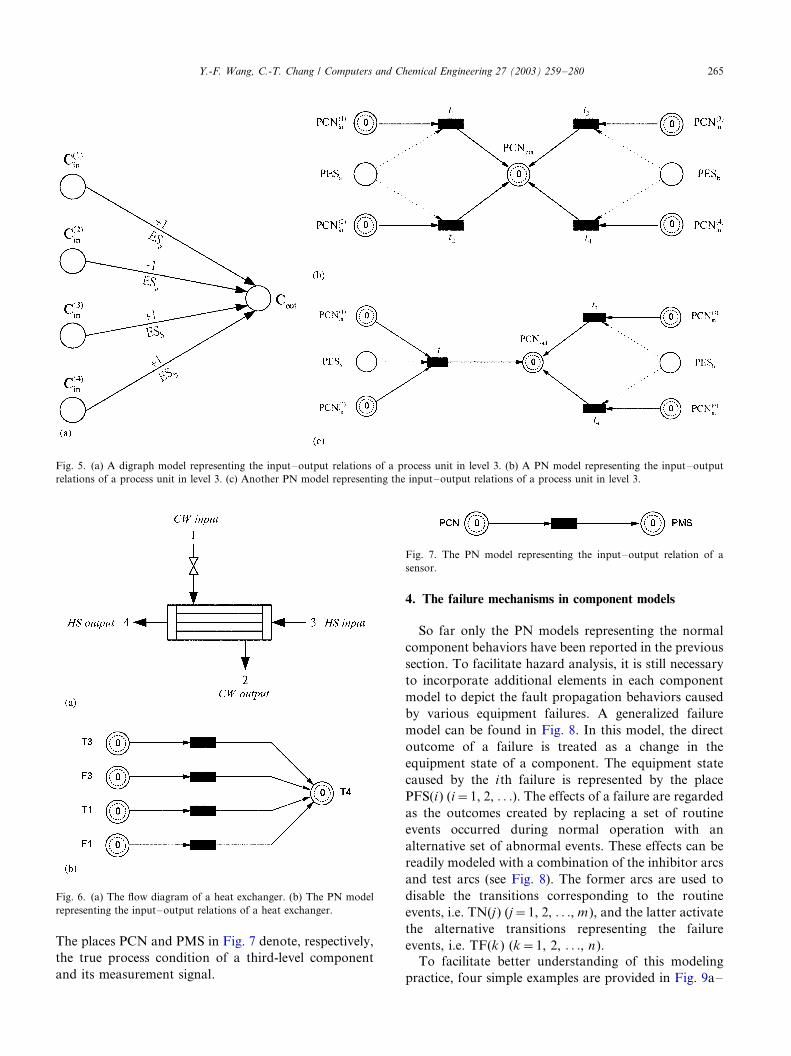
process unit, i.e. a heat exchanger in which a hot stream

HS is cooled with the cooling water CW (see Fig. 6a).

The qualitative model representing a part of its input�/

output conditions can be found in Fig. 6b.

3.4. Level 4

The equipment states and/or input�/output conditions

of a third-level component can be monitored via sensors

in the fourth level. Notice that there is no need to model

the equipment state of a sensor since it is always in theworking state during normal operation. The input�/

output relation of any sensor can also be represented

with a special version of Fig. 5b, i.e. the PN in Fig. 7.

Fig. 4. The generalized PN model describing the equipment state of a process unit in level 3.


The places PCN and PMS in Fig. 7 denote, respectively,

the true process condition of a third-level component

and its measurement signal.

4. The failure mechanisms in component models

So far only the PN models representing the normal

component behaviors have been reported in the previous

section. To facilitate hazard analysis, it is still necessary

to incorporate additional elements in each component

model to depict the fault propagation behaviors caused

by various equipment failures. A generalized failure

model can be found in Fig. 8. In this model, the direct

outcome of a failure is treated as a change in the

equipment state of a component. The equipment state

caused by the ith failure is represented by the place

PFS(i) (i�/1, 2, . . .). The effects of a failure are regarded

as the outcomes created by replacing a set of routine

events occurred during normal operation with an

alternative set of abnormal events. These effects can be

readily modeled with a combination of the inhibitor arcs

and test arcs (see Fig. 8). The former arcs are used to

disable the transitions corresponding to the routine

events, i.e. TN(j ) (j�/1, 2, . . ., m ), and the latter activate

the alternative transitions representing the failure

events, i.e. TF(k ) (k�/1, 2, . . ., n).

To facilitate better understanding of this modeling

practice, four simple examples are provided in Fig. 9a�/

Fig. 5. (a) A digraph model representing the input�/output relations of a process unit in level 3. (b) A PN model representing the input�/output

relations of a process unit in level 3. (c) Another PN model representing the input�/output relations of a process unit in level 3.

Fig. 6. (a) The flow diagram of a heat exchanger. (b) The PN model

representing the input�/output relations of a heat exchanger.

Fig. 7. The PN model representing the input�/output relation of a

sensor.


d. Following is a brief description of these failure

models:

. A controller/operator failure is described in Fig. 9a,

i.e. an extra operation step is carried out mistakenly.

Notice that the generalized model for the normal

control/operator behaviors (Fig. 1a) is repeated here

and, for the sake of clarity, the corresponding failure

model is enclosed with dotted line. In this case, the

place PC?(k ) and the transition TS?(k ) denote,

respectively, the status of the extra operation com-

mand and the event of issuing this command.

. The Petri net in Fig. 9b represents the fault propaga-

tion mechanism resulting from the failure ‘3-way

valve sticking.’ Again the PN used for modeling

normal operation (Fig. 2b) is included here and the

failure model is marked with dotted line. The

transitions denoting the valve-switching events, i.e.

TV(1) and TV(2), are disabled by inserting a token in

the place denoting the valve failure.

. The effects of ‘heat exchanger fouling’ on the output

temperature of hot stream arc modeled in Fig. 9c.

This failure causes a disruption of the normal

equipment state arid also an increase in the outlet

temperature, i.e. T4(�/1).

. The failure ‘temperature sensor failing low’ can be

described with a modeling approach similar to that in

the previous example. The corresponding Petri net is

presented in Fig. 9d. Notice that, other than the

obvious consequence that the sensor is no longer in

its normal equipment state, this failure yields a lower-

than-normal measurement value while the true tem-

perature is still kept at the normal level. In otherwords, the token number in the deviation place Tmeas

may be �/1 when that in Ttrue is still 0.

5. The model construction procedure

In building a PN-based system model for hazard

analysis, the component models should be constructed

and validated first and then connected in sequence from

top to bottom level according to the piping and

instrumentation diagram. The connection between two

adjacent component models can be described with Fig.10. Basically, the output conditions and, in some cases,

the equipment states of a downstream component are

controlled by the output conditions of an up-stream

component. However, if the equipment states of a third-

level component are time-variant, the transient beha-

viors of these states may also be affected by its operation

mode, which is uniquely defined by the equipment states

of one or more level-2 component.In principle, all component models should be included

to ensure the comprehensiveness of analysis. However,

some of them may be excluded for the sake of simplicity.

Specifically, a component can be neglected if:

1) its failure mechanisms are not of interest;

2) there is only one normal equipment state, and;

3) it is a single-input-and-single-output (SISO) com-

ponent.

Finally, it should be noted that the validity of the

system model can be confirmed by testing it with known

scenarios. In other words, the equipment states andprocess conditions of every component at different stage

of the batch operation should be simulated and com-

pared with the expected system behavior before actual

implementation of the proposed hazard identification

procedure.

Let us use, the simple mixing process given in Fig. 11

as an example to illustrate the proposed model con-

struction procedure. Here, tank 3 is being fed from theother two tanks. Initially, the amount of liquid A in tank

1 is 1 l and that of liquid B in tank 2 is 2 l. The mixing

operation begins when valve V1 and valve V2 are

opened by an operator. It is assumed that the flow rates

of these two feed streams are the same: 1/60 l/s. The

operator is instructed to close valve V2 whenever tank 1

is empty (step 1) or vice versa (step 2). The PN model for

this batch operation can be found in Fig. 12.The first-level component is the operator. For simpli-

city, only the two operation steps performed after

opening V1 and V2 are modeled here. Since they are

Fig. 8. A generalized failure model.


not required to be carried out in a specific order, the

input and output places associated with each step, i.e.

PS(i ) and PC(i ) (i�/1, 2), can be merged to simplify the

model structure.

There are two components in the second level, i.e.

valves V1 and V2. Their equipment states can be

described with two discrete places denoting ‘open’ and

‘closed.’ Two types of valve failures are considered in

this example, i.e. sticking and failing closed. The

corresponding failure models are included in this PN.

If the event ‘valve sticking’ occurs, it always disables a

transition representing the action to change valve

position. The corresponding token is, therefore, locked

in its input place. On the other hand, if a valve is

originally open and the event ‘valve failing closed’

occurs during operation, such a failure always moves

the token from the place representing the open position

to the other place denoting the opposite valve state.

The tanks in this example are the third-level compo-

nents. To characterize their equipment states, it is

necessary to trace the variations of the liquid levels in

all three tanks. Three continuous places are thus

adopted to represent these state variables. Notice that

the dead times of all time-delayed transitions are set to 1

s. Consequently, the weights on the output arcs from

and input arcs to these continuous places should be 1/60,

which is the same as the normal flow rate. The discrete

places F1 and F2 are used to reflect the output

conditions of Tank 1 and 2, respectively. If the flow

rate from Tank 1 (or Tank 2) to Tank 3 is maintained at

a normal level, then a token should be introduced into

the place F1 (or F2).

In this example, the possibility of sensor failures is

excluded and the sensor measurements are assumed to

be identical to the equipment states of Tank 1 and 2. As

a result, the sensor models can be omitted. It is also

assumed that the required mixing ratio of A�/B is 1.

Thus, an off-spec product may be produced if the

amounts of A and B in Tank 3 are not equal. This

undesirable outcome is flagged with a discrete place in

Fig. 12.

Fig. 9. (a) A failure model of the operator/controller. (b) A failure model of the 3-way valve. (c) A failure model of the heat exchanger. (d) A failure

model of the sensor.


The fault propagation behaviors resulting from the

valve failures given in Fig. 12 have been simulated with

an existing commercial software VISUAL OBJECT NET�/�/

(Drath, 1998a). Initially, all places are empty except the

two continuous places representing the amounts of

materials in Tanks 1 and 2. Their initial marks are 1.0

and 2.0, respectively. The failures were introduced later

in simulation. For the undesirable condition ‘off-spec

product,’ the simulation results can be found in Tables 3

and 4. It is clear from these results that the causes for thecondition ‘off-spec product’ occurring between 0 and 1

min are {valve V1 failing close between 0 and 1 min}

and {valve V2 failing close between 0 and 1 min} and

the cause for the same condition occurring between 1

and 2 min is {valve V2 sticking between 0 and 1 min}.

6. The object-oriented abbreviations

Strictly speaking, the PN models constructed with the

above procedure are only suitable for analyzing small

systems with moderately complex recipes. This is mainly

due to state-space explosion caused by the need to

describe not only the process configurations but also the

operation steps in an industrial-size system model. More

specifically, the total number of places and transitionstends to be overwhelmingly large in the corresponding

Petri nets. In order to handle this practical problem, the

object-oriented abbreviations (Drath, 1998b) have been

utilized in this study to simplify model structure and to

reduce the model-building effort. The inherent charac-

teristics of those abbreviations satisfy the basic needs in

constructing realistic models for sequential operations,

e.g. encapsulation, abstraction, inheritance, reusing,information hiding and message passing, etc.

As mentioned previously, a complete system model

consists of a large number of interacting components.

Fig. 9 (Continued)

Fig. 10. The connection between two adjacent component models.

Fig. 11. The process flow diagram of a mixing process.


Each component can be treated as an object. Basically,

every object can be fabricated according to a three-layer

structure. In the upper layer, it is only necessary to build

an object frame. For illustration clarity, this object

frame is always labeled with a heading and equipped

with multiple interface ports. Generally speaking, the

input and output ports can be configured according to

Fig. 10. The inputs should be taken from the output

ports of its up-stream objects and the outputs should be

passed to the input ports of its downstream objects.

There are two connected sub-frames in the underlying

second layer. They are used to encapsulate the PNs in

the bottom layer for describing equipment states and

input�/output conditions, respectively. The structures of

these two sub-frames are essentially identical to that of

the object frame. The outputs from the first, i.e. the

equipment states, are used as inputs to the second sub-

frame. The input and output ports on the object frame

in the upper layer are connected to those on these sub-

frames in the middle layer. As an example, the object

frame for a 3-way valve and its two sub-frames can be

found in Fig. 13a. The sub-frames and the encapsulated

PNs representing the equipment states and input�/out-

put conditions of the 3-way valve can be found in Fig.

13b and c, respectively.

7. Application

A practical example concerning an air-drying process

is presented here to demonstrate the feasibility of the

proposed model construction procedure and the useful-

ness of PN models in hazard assessment for the

sequential operations. Although a detailed description

of this process can be found in Shaeiwitz, Lapp and

Powers (1977), a brief review is still provided in the

sequel for the sake of completeness.

Fig. 12. The PN model of a mixing process.

Table 3

Simulation results of ‘valve sticking’ in mixing process

Valve number Failure time (u ) Occurrence time of ‘off-spec product’ Final valve state

V1 0BuB1 �/ V1: open

1BuB2 �/ V2: closed

V2 0BuB1 �1 V1: closed

V2: open

1BuB2 �/ V1: open

V2: closed


7.1. Process description

Fig. 14 is the flow diagram of a sequential process for

drying air by using fixed alumina beds. Ambient air,

which contains water vapor enters in stream 9, The airpasses through a bed of alumina, where the water vapor

is adsorbed. The dried air passes out of the process in

stream 25. In order to maintain a continuous supply of

dry air, two beds are employed. When one bed is

removing water from air, the other is being regenerated

and then cooled. Regeneration involves passing hot air

through a bed, which has been loaded to capacity with

water. The hot air strips the water from the alumina.After leaving the regenerating bed, it is then passed

through a cooler and a separator in turn to remove the

water vapor. Eventually, this air is recycled through the

lower port of the proportionating Valve and sent to the

bed currently in service. The regenerated bed must then

be cooled with the inlet air for a specific time period

before returning to its intended air-drying operation.

Both beds experience the same operation cycle. Table5 gives the detailed recipe in a complete cycle.

7.2. Model construction

The proposed model construction procedure can be

followed to build the PN for hazard analysis. Following

is a brief description of the component models in each

level.

7.2.1. Level 1

The first-level component in this system is the timer,which can be viewed as a device consisting of a

controller with an internal clock. The component model

for describing its normal behaviors can be assembled by

combining the two Petri nets in Fig. 1a and b (n�/4).

There are two timer failures considered in this study.

One is concerned with the controller. Notice from Table

5 that the 4-way valves are turned every two operation

periods when the initialization signals are generated bythe clock at the starting times of periods 1 and 3. It is

assumed that erroneous operation commands may be

issued by the controller to switch one or both of them to

the other position when period 2 or 4 begins. The

corresponding failure model can be found in Fig. 9a.

The other timer failure studied in this example is due to

clock malfunction. It is assumed that this clock stop

producing initiation signals should such an event occur.This failure can be modeled with inhibitor arcs pointing

to the transitions TC(i )s (i�/1, 2, 3, 4) in Fig. 1b.

7.2.2. Level 2

The second-level components are the 3-way valve 3W

and the two 4-way valves 4W-I and 4W-II. The

equipment states of these three valves can determine

the system configuration. The position of valve 3W

determines the route of inlet air flow. The fresh air caneither be directed to the heater or simply bypass it. The

position of valve 4W-I defines the connections between

the alumina beds and their air supplies. The air

consumed in each bed can be taken either from system

inlet (for regeneration or cooling) or from the lower port

of proportionating valve (for dehumidification). The

position of valve 4W-II governs the destinations of the

exit airs from these two beds, i.e. the air can be eitherdischarged or recycled.

Every valve in this system can only be switched to two

alternative positions, i.e. PV(�/) and PV(�/). The

relationships between the valve positions and the stream

connections are shown in Table 6. The model structures

for these three valves are essentially the same. The

equipment states of a normal valve can always be

represented with the Petri net presented in Fig. 2b.The failure model associated with ‘valve sticking’ can

then be attached according to Fig. 9b. The correspond-

ing model of the input�/output conditions can be built

on the basis of Fig. 3b. In this case, the relations

between the input and output temperatures and water

concentrations should also included in the same fashion.

Specifically, the PNs for these relations can be con-

structed according to Table 7.

7.2.3. Level 3

Six third-level components can be readily identified

from the P&ID given in Fig. 14, i.e. the two alumina

beds, the heater, the cooler, the separator and the

Table 4

Simulation results of ‘valve failing closed’ in mixing process

Valve number Failure time (u ) Occurrence time of ‘off-spec product’ Final valve state

V1 0BuB1 �u V1: closed

V2: open

1BuB2 �/ V1: closed

V2: closed

V2 0BuB1 �u V1: open

V2: closed

1BuB2 �/ V1: open

V2: closed


proportionating valve. In addition, the joint connecting

lines 16, 17 and 18 is also treated as a level-3 component

here. It is referred to as a mixer in this example. Other

than the beds, only one equipment state is needed to

characterize each level-3 component. The Petri nets

representing their qualitative input�/output relations

can be developed according to the model structure

presented in Fig. 5b. The correspondence between the

inputs and outputs of each one-state component is given

in Table 8. Notice that, instead of presenting the PN

models explicitly in this table, the edge gains in the

corresponding digraphs (see Fig. 5a) are specified for the

sake of conciseness.

The equipment states of each alumina bed can be

described with two parameters, i.e. the bed temperature

and water content. From a careful analysis of the

operation procedure for the air-drying process, it can

be observed that the main controlling factor of bed

temperature is the temperature of in-coming air. Within

one time period, hot air should raise the bed tempera-

ture until reaching an upper bound and, conversely, cool

air should decrease it to a lower limit. On the other

Fig. 13. (a) The object net of a 3-way valve. (b) The sub-object net of a 3-way valve (equipment state). (c) The sub-object net of a 3-way valve (input�/

output condition).


hand, the water content is a function of the temperature

of the inlet air and also the bed temperature. If both

temperatures are low and the bed is unsaturated, the

water content in alumina bed can be increased by

passing either fresh air from environment or recycled

air from the proportionating valve. Eventually, the

amount of water should reach a saturation level in at

most two time periods. A saturated bed cannot be used

for dehumidification purpose. Therefore, hot air should

be introduced in the adsorption beds to strip water from

the alumina. Here, it is assumed that the bed can be

dried ‘completely’ in one time period.

From the above discussions, it is clear that the

equipment states of an alumina bed are manipulated

in this system by switching from one operation mode to

another each time when a new period begins. These

operation modes can be instituted by adjusting the

positions of 3-way and 4-way valves according to Table

9. In this table, the symbols H, C, P, E and R represent

different operation modes of an alumina bed. The first

three are concerned with the input connections of the

bed. In particular, H is used to represent the facts that

the in-coming air is taken from environment and it is

pre-heated; C denotes that cool fresh air is used in bed; P

indicates that the entering air is obtained from the

proportionating valve. Notice that these modes are

defined by the positions of the 3-way valve 3W and

the first 4-way valve 4W-I. On the other hand, the last

two labels reflect the output connections. As mentioned

Fig. 14. The process flow diagram of a utility air drying process (Shaeiwitz et al., 1977).

Table 5

Operating procedure for fixed-bed air drying system

Time period Valve position Bed status

3W 4W-I 4W-II Bed-I Bed-II

1 11012 18019 20021 Regeneration In service

22023 24025

2 11017 18019 20021 Cooling In service

22023 24025

3 11012 18023 20025 In service Regeneration

22019 24021

4 11017 18023 20025 In service Cooling

22019 24021

Table 6

The relationships between valve positions and stream connections

Valve Valve position Stream connection

3W � 11012

� 11017

4W-I � 18019 and 22023

� 18023 and 22019

4W-II � 20021 and 24025

� 20025 and 24021


before, these connections are governed by the second 4-

way valve 4W-II. Specifically, the out-going air can be

either recycled (R) or sent downstream (E).

Since the equipment states of an alumina bed is

independent of the output conditions, the corresponding

PN model can be constructed by considering only theoperation modes listed in the first four rows of Table 9.

Although the bed temperature and water content are

basically continuous quantities, a discrete version of Fig.

4 is employed here to represent their transient behaviors

qualitatively. This practice is adopted mainly to reduce

model complexity. As an example, let us consider the

Petri net for the equipment states of Bed-I (Fig. 15). The

discrete places I-T and I-M are used to represent the bedtemperature and water content, respectively. The num-

ber of tokens in each place denotes the qualitative value

of the corresponding parameter. An empty place

represents the parameter is at its lowest level. Its upper

limit can be set by the capacity, i.e. the maximum

allowable token number, of the same place. In this

example, the capacities of I-T and I-M are 1 and 2,

respectively. A token in the place I-M denotes that thewater content in Bed-I is ‘partially’ saturated. The other

three discrete places, i.e. I-H, I-C and I-P, are used to

represent the three operation modes listed in the first

four rows of Table 9. Notice that the prefix ‘I’ in this

Petri net indicates that this model is associated with

Bed-I. The PN model for the equipment states of Bed-II

can be obtained simply by adopting ‘II’ as the prefix of

each place in Fig. 15.For the alumina beds, the qualitative causal relations

of input and output conditions are dependent upon not

only the equipment states but also the operation modes.

During normal operation, the input connections and

initial states of Bed-I in each time period can be

characterized with the token numbers in I-H, I-C, I-P,

I-T and I-M (see Table 10). Since the bed temperature,

water content and also input air temperature in the fourtime periods are not the same, different input�/output

models should be adopted accordingly. Furthermore, in

addition to the conditions listed in Table 10, there are

other possible scenarios which may be encountered

Table 7

The inputs and outputs of the second-level component models

Component Equipment state Input Output

3-Way valve � F11 F12

T11 T12

C11 C12

� F11 F17

T11 T17

C11 C17

4-Way valve (I) � F18 F19

T18 T19

C18 C19

F22 F23

T22 T23

C22 C23

� F18 F23

T18 T23

C18 C23

F22 F19

T22 T19

C22 C19

4-Way valve (II) � F20 F21

T20 T21

C20 C21

F24 F25

T24 T25

C24 C25

� F20 F25

T20 T25

C20 C25

F24 F21

T24 T21

C24 C21

Table 8

The input�/output relations of the one-state level-3 components

Component Input Output Edge gain

Proportionating valve F7 F11,F22 �1, �1

T7 T22 �1

C7 C22 �1

F9 F11, F22 �1, �1

T9 T11,T22 �1, �1

C9 C11,C22 �1, �1

Mixer F16 F18 �1

T16 T18 �1

C16 C18 �1

F17 F18 �1

T17 T18 �1

C17 C18 �1

Air heater F12 F16,T16 �1, �1

T12 T16 �1

C12 C16 �1

F13 T16 �1

T13 T16 �1

Cooler F21 F3,T3,C3 �1, �1, �1

T21 T3,C3 �1, �l

C21 C3 �1

F1 T3,C3 �1, �1

T1 T3,C3 �1, �1

Separator F3 F7 �1

T3 T7,C7 �1, �1

C3 C7 �1

Table 9

The relationships between valve positions and bed operation modes

Valve positions Operation modes

3W 4W-I 4W-II Bed-I Bed-II

� � H P

� � C P

� � P H

� � P C

� R E

� E R


during abnormal operations. To facilitate hazard ana-

lysis, it is also necessary to develop the corresponding

input�/output models. From the facts that (1) the

operation modes I-H, I-C and I-P are mutually exclusive

and (2) there are only two possible token numbers in I-T

(i.e. 0 and 1) and 3 in I-M (i.e. 0, 1, 2), it can be deduced

that the number of all possible combinations should be

18. In this example, these conditions are classified into

five groups according to Table 11 and the corresponding

models are presented in the first part of Table 12. Notice

that the values specified in the brackets in Table 11 are

the token numbers in the corresponding places. It can be

seen that the conditions listed in Table 10 are also

embedded in Table 11. Thus, models 1 and 2 in Table 12

can be used under the normal operating conditions

during time period 1 and 2, respectively, and model 3

can be used for the normal operation in both periods 3

and 4. Finally, it should be noted the input�/output

relations of Bed-II can be classified on the basis of Table

11. In particular, every prefix ‘I’ in this table should be

replaced with an ‘II’.

Finally, all level-3 component failures considered inthis example are listed in the third column of Table 13.

Each failure can be described according to the model

structure in Fig. 9c.

7.2.4. Level 4

It is assumed in this example that the measurement

instruments are not used in implementing the operation

procedure. Consequently, all level-4 component models

are neglected.

7.2.4.1. The complete system model. All componentmodels can be encapsulated in object frames and then

connected according to the P&ID presented in Fig. 14.

The resulting system model can be found in Fig. 16.

Fig. 15. The PN model describing the equipment states of Bed-I.

Table 10

The input connections and initial states of Bed-I in each time period

Time period I-H I-C I-P I-T I-M

1 1 0 0 0 2

2 0 1 0 1 0

3 0 0 1 0 0

4 0 0 1 0 1

Table 11

The input�/output relations of Bed-I

Model number Model conditions

1 I-H[1]�I-T[0]�I-M[1,2]

2 I-C[1]�I-T[1]�I-M[0,1,2]

I-P[1]�I-T[1]�I-M[0,1,2]

3 I-P[1]�I-T[0]�I-M[0,1]

I-C[1]�I-T[0]�I-M[0,1]

4 I-C[1]�I-T[0]�I-M[2]

I-P[1]�I-T[0]�I-M[2]

5 I-H[1]�I-T[0]�I-M[0]

I-H[1]�I-T[1]�I-M[0,1,2]

Table 12

The input�/output relations of the multi-states level-3 components

Component Model num-

ber

Input Output Gain

Alumina Bed (I) 1 F19 F20,T20,C20 �1, �1,

�1

T19 T20,C20 �1, �1

C19 C20 �1

2 F19 F20,T20 �1, �1

T19 T20 �1

C19 C20 �1

3 F19 F20,C20 �1, �1

T19 T20,C20 �1, �1

C19 C20 �1

4 F19 F20 �1

T19 T20 �1

C19 C20 �1

5 F19 F20,T20 �1, �1

T19 T20 �1

C19 C20 �1

Alumina Bed (II) 1 F23 F24,T24,C24 �1, �1,

�1

T23 T24,C24 �1, �1

C23 C24 �1

2 F23 F24,T24 �1, �1

T23 T24 �1

C23 C24 �1

3 F23 F24,C24 �1, �1

T23 T24,C24 �1, �1

C23 C24 �1

4 F23 F24 �1

T23 T24 �1

C23 C24 �1

5 F23 F24,T24 �1, �1

T23 T24 �1

C23 C24 �1


Table 13

The failure models of level-3 components

Component Model number Failure Output deviation

Proportionating valve �/ Failing height F11(�1), F22(�1)

Air heater �/ Steam leak into air F16(�1), T16(�1), C16(�1)

Cooler �/ External fire T3(�1), C3(�1)

Separator �/ Trap plugged F7(�1), C7(�1)

Alumina Bed (I) 1 Channeling T20(�1), C20(�1)

Leak out F20(�1)

2 Channeling T20(�1)

Leak out F20(�1)

3 Channeling C20(�1)

Leak out F20(�1), C20(�1)

Alumina Bed (II) 1 Channeling T24(�1), C24(�1)

Leak out F24(�1)

2 Channeling T24(�1)

Leak out F24(�1)

3 Channeling C24(�1)

Leak out F24(�1), C24(�1)

Fig. 16. The complete PN model of a utility air drying process.


7.3. Auxiliary devices

The fault propagation behaviors caused by all possi-

ble combinations of failures and/or disturbances are

simulated with the Petri net presented in Fig. 16.

Obviously, an extremely large number of case studies

must be carried out for a comprehensive hazard

analysis. It is, therefore, necessary to install additional

auxiliary devices in this PN model to facilitate efficient

and systematic implementation. These auxiliary devices

are described as follows.

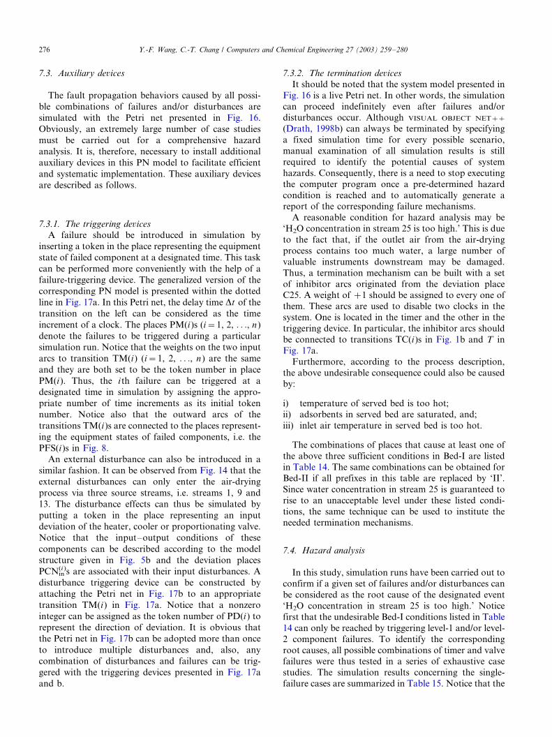
7.3.1. The triggering devices

A failure should be introduced in simulation by

inserting a token in the place representing the equipment

state of failed component at a designated time. This task

can be performed more conveniently with the help of a

failure-triggering device. The generalized version of the

corresponding PN model is presented within the dotted

line in Fig. 17a. In this Petri net, the delay time Dt of the

transition on the left can be considered as the time

increment of a clock. The places PM(i)s (i�/1, 2, . . ., n )

denote the failures to be triggered during a particular

simulation run. Notice that the weights on the two input

arcs to transition TM(i) (i�/1, 2, . . ., n ) are the same

and they are both set to be the token number in place

PM(i ). Thus, the ith failure can be triggered at a

designated time in simulation by assigning the appro-

priate number of time increments as its initial token

number. Notice also that the outward arcs of the

transitions TM(i )s are connected to the places represent-

ing the equipment states of failed components, i.e. the

PFS(i )s in Fig. 8.

An external disturbance can also be introduced in a

similar fashion. It can be observed from Fig. 14 that the

external disturbances can only enter the air-drying

process via three source streams, i.e. streams 1, 9 and

13. The disturbance effects can thus be simulated by

putting a token in the place representing an input

deviation of the heater, cooler or proportionating valve.

Notice that the input�/output conditions of these

components can be described according to the model

structure given in Fig. 5b and the deviation places

PCNin(i )s are associated with their input disturbances. A

disturbance triggering device can be constructed by

attaching the Petri net in Fig. 17b to an appropriate

transition TM(i) in Fig. 17a. Notice that a nonzero

integer can be assigned as the token number of PD(i ) to

represent the direction of deviation. It is obvious that

the Petri net in Fig. 17b can be adopted more than once

to introduce multiple disturbances and, also, any

combination of disturbances and failures can be trig-

gered with the triggering devices presented in Fig. 17a

and b.

7.3.2. The termination devices

It should be noted that the system model presented in

Fig. 16 is a live Petri net. In other words, the simulation

can proceed indefinitely even after failures and/ordisturbances occur. Although VISUAL OBJECT NET�/�/

(Drath, 1998b) can always be terminated by specifying

a fixed simulation time for every possible scenario,

manual examination of all simulation results is still

required to identify the potential causes of system

hazards. Consequently, there is a need to stop executing

the computer program once a pre-determined hazard

condition is reached and to automatically generate areport of the corresponding failure mechanisms.

A reasonable condition for hazard analysis may be

‘H2O concentration in stream 25 is too high.’ This is due

to the fact that, if the outlet air from the air-drying

process contains too much water, a large number of

valuable instruments downstream may be damaged.

Thus, a termination mechanism can be built with a set

of inhibitor arcs originated from the deviation placeC25. A weight of �/1 should be assigned to every one of

them. These arcs are used to disable two clocks in the

system. One is located in the timer and the other in the

triggering device. In particular, the inhibitor arcs should

be connected to transitions TC(i)s in Fig. 1b and T in

Fig. 17a.

Furthermore, according to the process description,

the above undesirable consequence could also be causedby:

i) temperature of served bed is too hot;ii) adsorbents in served bed are saturated, and;

iii) inlet air temperature in served bed is too hot.

The combinations of places that cause at least one of

the above three sufficient conditions in Bed-I are listed

in Table 14. The same combinations can be obtained for

Bed-II if all prefixes in this table are replaced by ‘II’.

Since water concentration in stream 25 is guaranteed to

rise to an unacceptable level under these listed condi-

tions, the same technique can be used to institute theneeded termination mechanisms.

7.4. Hazard analysis

In this study, simulation runs have been carried out to

confirm if a given set of failures and/or disturbances can

be considered as the root cause of the designated event

‘H2O concentration in stream 25 is too high.’ Notice

first that the undesirable Bed-I conditions listed in Table

14 can only be reached by triggering level-1 and/or level-

2 component failures. To identify the corresponding

root causes, all possible combinations of timer and valvefailures were thus tested in a series of exhaustive case

studies. The simulation results concerning the single-

failure cases are summarized in Table 15. Notice that the


occurrence times of the designated event are specified in

the second column, and the root causes and their

triggering times are provided in the third column. Let

us consider two scenarios resulting from the failure

‘valve 3W sticking’ as examples, i.e. rows 7 and 10. If

valve 3W sticks in period 1, the inlet air for regeneration

should pass through the heater in period 2. Thus, the

regenerated bed is not cooled in the same period.

Because of the fact that condition (i) is satisfied, the

designated undesirable condition should occur in the

next time period. On the other hand, if valve 3W sticks

in period 4, the inlet air for cooling should bypass the

heater in period 1 in the next cycle and thus Bed-I

cannot be regenerated. When the alumina bed is in

service during period 3 in the next cycle, it should still be

saturated with water. Since condition (ii) is satisfied, the

designated undesirable condition is bound to occur in

this period.

Naturally, the above condition may also be the result

of various combinations of multiple timer and valve

failures. All 2-failure and 3-failure scenarios resulting in

Fig. 17. (a) The failure triggering device. (b) The disturbance triggering device.

Table 14

The outcome places associated with the sufficient conditions of

undesirable consequence ‘C25(�1)’

Sufficient conditions Outcome places

(i) I-H[1]�I-E[1]�I-T[1]�I-M[0,1,2]

I-C[1]�I-E[1]�I-T[1]�I-M[0,1,2]

I-P[1]�I-E[1]�I-T[1]�I-M[0,1,2]

(ii) I-H[1]�I-E[1]�I-T[0,1]�I-M[2]

I-C[1]�I-E[1]�I-T[0,1]�I-M[2]

I-P[1]�I-E[1]�I-T[0,1]�I-M[2]

(iii) I-H[1]�I-E[1]�I-T[0,1]�I-M[0,1,2]


the undesirable Bed-I conditions in Table 14 are

presented in Tables 16 and 17, respectively. Let us

consider the root causes shown in the 1st row of Table

16 in detail. If valve 3W sticks in period 1, the system

should behave normally during the same period. If, in

addition, valve 4W-II is abnormally reversed in period 2,

the inlet air should be misdirected to Bed-I and it is still

hot due to 3W sticking. Thus, the outlet air from Bed-I

must be discharged to stream 25. Hence, the tempera-

ture and moisture content in stream 25 should be

abnormally high in period 2.As mentioned before, the level-1 and level-2 compo-

nent failures reported in Tables 15�/17 are only the root

causes of the abnormal Bed-I states listed in Table 14. It

should be noted that the undesirable consequence ‘H2O

concentration in stream 25 is too high’ may also be

attributed to Bed-II conditions. These missing root

causes can be easily recreated by subtracting two periods

from the occurrence times listed in the second and third

columns of Tables 15�/17. Notice also that the advan-

tages of the Petri net, models can be clearly observed

from a comparison between the above results and those

obtained with digraphs. Specifically, the fault propaga-

tion scenarios identified by Shaeiwitz et al. (1977) are

limited to only the cases in which the basic and top

events occur in the same operation period. In other

words, the possibilities of earlier failure(s) causing the

designated undesirable consequence in a later time

period are not considered in the conventional fault-

tree analysis. This restriction can be successfully re-

moved with Petri nets in the present work.

Since the above scenarios are only concerned with

level-1 and/or level-2 component failures, it is still

necessary to examine other possibilities, i.e. the external

disturbances and the level-3 component failures. From

the P&ID presented in Fig. 14, it is clear that changes in

the upstream conditions, i.e. flow rate, temperature or

H2O concentration, can be introduced into cooling

water (stream 1), inlet air (stream 9) and steam (stream

13). Simulation runs can thus be carried out by installing

Table 15

The single-failure causes involving level-1 and level-2 components

Outcome places Occurrence

time

Root causes

I-H[1]�I-E[1]�I-

T[0]�I-M[0]

(3) Spurious controller command

to 4W-I (2)

(3) 4W-I sticking (1)

(3) 4W-I sticking (2)

I-H[1]�I-E[1]�I-

T[0]�I-M[2]

(1) 4W-II sticking (3)

(1) 4W-II sticking (4)

I-C[1]�I-E[1]�I-

T[1]�I-M[0]

(2) Spurious controller command

to 4W-II (2)

I-P[1]�I-E[1]�I-

T[1]�I-M[0]

(3) 3W sticking (1)

I-P[1]�I-E[1]�I-

T[0]�I-M[2]

(1) Clock failing off (3)

(1) Clock failing off (4)

(3) 3W sticking (4)

Table 16

The 2-failure causes involving level-1 and level-2 components

Outcome places Occurrence

time

Root causes

I-H[1]�I-E[1]�I-

T[1]�I-M[0]

(2) 3W sticking (1), spurious con-

troller command to 4W-II (2)

(3) 3W sticking (1), 4W-I sticking (1)


I-H[1]�I-E[1]�I-

T[0]�I-M[1]


troller command to 4W-I (4)

I-C[1]�I-E[1]�I-

T[0]�I-M[2]

(1) 4W-II sticking (3), 3W sticking (4)

(1) 3W sticking (2), 4W-II sticking (3)




troller command to 4W-II (2)







I-P[1]�I-E[1]�I-

T[1]�I-M[0]

(2) Spurious controller command to

4W-I (2) and 4W-II (2)

I-P[1]�I-E[1]�I-

T[0]�I-M[2]

(1) 4W-I sticking (3), 4W-II sticking

(3)


(4)


(4)

(1) 4W-II sticking (3), 4W-I sticking

(4)

(1) 4W-II sticking (3), spurious con-


(1) 4W-II sticking (4), spurious con-


Table 17

The 3-failure causes involving level-1 and level-2 components

Occurrence

time

Root causes

(1) 3W sticking (2), spurious controller command to 4W-

I (2), 4W-II sticking (3)


I (2), 4W-II sticking (4)

(2) 3W sticking (4), 4W-I sticking (4), spurious controller

command to 4W-II (2)


I (2), spurious controller command to 4W-II (2)

(2) 4W-I sticking (3), 3W sticking (4), spurious controller

command to 4W-II (2)

(2) Spurious controller command to 4W-I (4), 3W

sticking (4), spurious controller command to 4W-II

(2)


the disturbance-triggering devices in Fig. 17a and baccordingly. It can be observed that the undesirable

consequence can be caused by any of the following seven

external disturbances during the same operation period;

(1) F1(�/1); (2) T1(�/1); (3) F9(�/1); (4) T9(�/1); (5)

C9(�/1); (6) F13(�/1); and (7) T13(�/1). On the other

hand, the effects of level-3 component failures in Table

13 can also be assessed by simulation. Notice that each

component failure can be modeled on the basis of Fig.9c. The effects of these failures can be introduced in

simulation using the failure-triggering device presented

in Fig. 17a. It was found that an increase in the H2O

concentration of stream 25 can be caused by any of the

following five level-3 component failures during the

same operation period:

1) proportionating valve failing high;

2) external fire near cooler;

3) separator trap plugged;4) Bed-I channeling in period 3 and 4;

5) Bed-II channeling in period 1 and 2.

Finally, it should be noted that the possibility of the

designated undesirable consequence cannot be ruled out

even if it does not occur during the same period in which

a disturbance or level-3 component failure is introduced.

The corresponding fault propagation behaviors in later

time periods can be easily simulated with the proposed

system model. In order words, it is possible to trace fromthe event ‘C25(�/1)’ to its root causes occurred in earlier

time periods. Since the detailed discussions of these

more subtle cases are quite lengthy, they are not

included in the present paper for the sake of brevity.

8. Conclusions

A hierarchical approach is proposed in this study to

construct a comprehensive PN model for any sequential

operation. Systematic simulation techniques are also

developed to describe the effects of a given set ofcomponent failures and/or external disturbances. By

following the proposed methodology, identification and

enumeration of critical fault propagation scenarios

become very efficient. It is clear from the application

results that the proposed PN models can indeed be used

as the basis for rigorous hazard analysis.

Acknowledgements

This work is supported by the National Science

Council of the ROC government under Giant NSC89-

2214-E006-027.

Appendix A: The deviation places

The properties of a deviation place can be clearly

characterized with existing places and transitions. The

resulting Petri net is presented in Fig. 18. Notice that thetoken numbers allowed in the continuous place PCN,

here, are the same as those in the corresponding

deviation place. Furthermore, the Petri net in Fig. 18

can be divided into two distinct components by remov-

ing PCN. The component on the left can be regarded as

a ‘receiver.’ A token in the place IN indicates that its

input transition has been fired. The existing token

number in PCN is then replaced with a new one. Thisnewly received token number is determined according to

a user-supplied weight function W (+). The independent

variables of this function are the token numbers of the

upstream deviation places. Basically, any desired input�/

output relation can be specified with W (+). On the other

hand, the component on the right can be considered as

an ‘activator,’ To facilitate simulation of the propaga-

tion behaviors of external disturbances, a continuousplace PREC is used, here, to store the old token number

in the deviation place before a new number is received in

PCN. In order to ensure that the fault propagation

Fig. 18. The PN model of a deviation place.


mechanism is activated only when the token numbers in

PCN and PREC are different, an inhibitor arc and a test

arc are attached to PCN as outputs to two separate

transitions. Notice the weight on the former arc isPREC. Thus, its output transition is enabled if the token

number in place PCN is less than that in place PREC.

Notice also that the weight on the latter arc is PREC�/1.

This implies that, its output transition is enabled only

when the token number in place PCN is greater than or

equal to that in place PREC. It is obvious from this

structure that only one of these two transitions can be

fired at any given time. After firing, the new tokennumber in PCN should be introduced into PREC to

replace the old one and, also, a token should be inserted

in place OUT to trigger its output transition.

References

Alla, H., & David, R. (1998). A modelling and analysis tool for

discrete events systems: continuous Petri net. Performnace

Evaluation 33 , 175.

Allen, D. J., & Rao, M. S. M. (1980). New algorithms for the synthesis

and analysis of fault trees. Industrial Engineering and Chemical

Fundamental 19 , 79.

Andrews, J. D., & Morgan, J. M. (1986). Application of digraph

method of fault tree construction to process plant. Reliable

Engineering 14 , 85.

Bowden, F. D. J. (2000). A brief survey and synthesis of the roles of

time in Petri nets. Mathematical and Computational Model 31 , 55.

Chang, C. T., & Hwang, H. C. (1992). New development of the

digraph-based techniques for fault-tree synthesis. Industrial En-

gineering Chemical Research 31 , 1490.

Chang, C. T., & Hwang, K. S. (1994). Studies on the digraph-based

approach for fault-tree synthesis 1, the ratio-control systems.

Industrial Engineering and Chemical Research 33 , 1520.

Chang, C. T., Hsu, D. S., & Hwang, D. M. (1994). Studies on the

digraph-based approach for fault-tree synthesis 2, the trip systems.

Industrial Engineering and Chemical Research 33 , 1700.

David, R. (1997). Modeling of hybrid systems using continuous and

hybrid Petri nets, Proceedings of the Seventh International Work-

shop on Petri Nets and Performance Models (p. 47). Saint Malo,

France.

David, R., & Alla, H. (1994). Petri net for modeling of dynamic

systems*/a survey. Automatica 30 (2), 175.

Drath, R. (1998a). URL http://www.systemtechnik.tu-ilmenau.de/--

drath.

Drath, R. (1998b). Hybrid object nets: An object oriented concept for

modeling complex hybrid systems. Proceeding of 3rd International

Conference on Automation of Mixed Processes: Hybrid Dynamical

Systems (p. 437). Reims.

Kelly, B. E., & Lees, F. P. (1986a). The propagation of faults in

process plants: 1, modeling of fault propagation. Reliable Engi-

neering 16 , 3.

Kelly, B. E., & Lees, F. P. (1986b). The propagation of faults in

process plants: 2, fault tree synthesis. Reliable Engineering 16 , 39.

Kumamoto, H., & Henley, E. J. (1979). Safety and reliability synthesis

of systems with control loops. American Institute of Chemical

Engineering Journal 20 , 376.

Lapp, S. A., & Powers, G. J. (1977). Computer-aided synthesis of

fault-trees. IEEE Transmission Reliable R-26 , 2.

Peterson, J. L. (1981). Petri net theory and the modeling of systems .

Englewood Cliffs, NJ: Prentico-Hall.

Petri, C. A. (1962), Kommunikation mit Automaten . Ph.D. thesis,

University of Bonn, Bonn, Germany.

Shaeiwitz, J. A., Lapp, S. A., & Powers, G. J. (1977). Fault tree

analysis of sequential systems. Industrial Engineering and Chemical

Process Description Development 16 (4), 529.

Srinivasan, R., & Venkatasubramanian, V. (1998a). Automating

HAZOP analysis of batch chemical plants: part i. the knowledge

representation framework. Computer and Chemical Engineering 22

(9), 1345.

Srinivasan, R., & Vonkatasubramanian, V. (1998b). Automating

HAZOP analysis of batch chemical plants: part ii. Algorithms

and application. Computer and Chemical Engineering 22 (9), 1357.

Szucs, A., Gerzson, M., & Hangos, K. (1998). An intelligent diagnostic

system based on Petri nets. Computer and Chemical Engineering 22

(9), 1335.

Vaidhyanathan, R., & Venkatasubramanian, V. (1996a). Haxop

expert: an expert system for automating HAZOP analysis. Process

Safe Programe 15 (2), 80.

Vaidhyanathan, R., & Venkatasubramanian, V. (1996b). A semi-

quantitative reasoning methodology for filtering and ranking

HAZOP results in HAZOP expert. Reliable Engineering and System

Safe 53 , 185.


http://www.systemtechnik.tu-ilmenau.de/-drath



Documents

A hierarchical approach to construct Petri nets for