Embed Size (px)
Citation preview
A Guide to Coordinate Systems in Great Britain
V3.3 © OS 2018
Page 1 of 53
G E O D E SY & PO S I T I O N I N G
A Guide to Coordinate
Systems in Great Britain
An introduction to mapping coordinate systems and the use of GNSS datasets with
Ordnance Survey mapping
A Guide to Coordinate Systems in Great Britain
V3.3 © OS 2018
Page 2 of 53
Contact Us
Ordnance Survey web site – www.os.uk
Customer Service Centre
Ordnance Survey
Adanac Drive
SOUTHAMPTON
United Kingdom
SO16 0AS
General enquiries: +44 (0)3456 05 05 05
Dedicated Welsh language Helpline: +44 (0)3456 05 05 04
Textphone : +44 (0)23 80 05 61 46
Trademarks
Ordnance Survey, OSGM15, OS Net and OSGB36 are registered trademarks and OS logos and
OSTN15 are trademarks of OS, Britain’s mapping agency.
All other trademarks are acknowledged.
Waiver
This document is made generally available by Ordnance Survey for free. As such it is provided 'as
is' and Ordnance Survey excludes all representations, warranties, obligations and liabilities in
relation to the document to the maximum extent permitted by law. Ordnance Survey shall not be
liable for any errors or omissions in this document and shall not be liable for any loss, injury or
damage of any kind caused by its use.
Acknowledgments
You are free to use this document under fair dealing or fair use or any other copyright exceptions.
Where you copy, publish or distribute the contents of this document to third parties, you must
acknowledge Ordnance Survey as the source of the information by including the attribution
statement ‘Copyright Ordnance Survey 2018’.
A Guide to Coordinate Systems in Great Britain
V3.3 © OS 2018
Page 3 of 53
Contents
Section Page no
1 Introduction ............................................................................................................................................. 5
1.1 Who should read this booklet? ....................................................................................................... 5
1.2 A few myths about coordinate systems ........................................................................................ 6
2 The shape of the Earth ............................................................................................................................ 8
2.1 The first geodetic question ............................................................................................................. 8
2.2 Ellipsoids........................................................................................................................................... 8
2.3 The geoid .......................................................................................................................................... 9
2.3.1 Local geoids ...................................................................................................................... 10
3 What is position...................................................................................................................................... 11
3.1 Types of coordinates ..................................................................................................................... 11
3.1.1 Latitude, longitude and ellipsoid height ........................................................................ 11
3.1.2 Cartesian coordinates ...................................................................................................... 13
3.1.3 Geoid height (also known as orthometric height) ........................................................ 13
3.1.4 Mean sea level height ....................................................................................................... 15
3.1.5 Eastings and northings .................................................................................................... 17
3.2 We need a datum ........................................................................................................................... 17
3.2.1 Datum definition before the space age .......................................................................... 18
3.3 Realising the datum definition with a Terrestrial Reference Frame ........................................ 19
3.4 Summary ........................................................................................................................................ 20
4 Modern GNSS coordinate systems....................................................................................................... 20
4.1 World Geodetic System 1984 (WGS84) ........................................................................................ 20
4.2 Realising WGS84 with a TRF ......................................................................................................... 22
4.2.1 The WGS84 broadcast TRF............................................................................................... 22
4.2.2 The International Terrestrial Reference Frame (ITRF) ................................................. 23
4.2.3 The International GNSS Service (IGS)............................................................................. 23
4.2.4 European Terrestrial Reference System 1989 (ETRS89)............................................... 24
5 Ordnance Survey coordinate systems................................................................................................. 26
5.1 ETRS89 realised through OS Net .................................................................................................. 26
5.2 National Grid and the OSGB36 TRF ............................................................................................. 27
5.2.1 The OSGB36 datum .......................................................................................................... 28
5.2.2 The OSGB36 TRF ............................................................................................................... 28
5.2.3 Relative accuracy of OSGB36 control points ................................................................. 29
5.3 Ordnance Datum Newlyn.............................................................................................................. 30
A Guide to Coordinate Systems in Great Britain
V3.3 © OS 2018
Page 4 of 53
5.3.1 The ODN datum ................................................................................................................ 30
5.3.2 The ODN TRF ..................................................................................................................... 31
5.3.3 Relative accuracy of ODN bench marks ......................................................................... 31
5.4 Other height datums in use across Great Britain ....................................................................... 32
5.5 The future of British mapping coordinate systems ................................................................... 32
6 From one coordinate system to another: geodetic transformations .............................................. 33
6.1 What is a geodetic transformation?............................................................................................. 33
6.2 Helmert datum transformations.................................................................................................. 35
6.3 National Grid Transformation OSTN15 (ETRS89–OSGB36) ...................................................... 38
6.4 National Geoid Model OSGM15 (ETRS89-Orthometric height) ................................................. 38
6.5 ETRS89 to and from ITRS .............................................................................................................. 39
6.6 Approximate WGS84 to OSGB36/ODN transformation ............................................................. 39
6.7 Transformation between OS Net v2001 and v2009 realisations .............................................. 40
7 Transverse Mercator map projections ................................................................................................ 41
7.1 The National Grid reference convention ..................................................................................... 42
8 Further information ............................................................................................................................... 43
A Datum, ellipsoid and projection information ..................................................................................... 44
A.1 Shape and size of biaxial ellipsoids used in the UK ................................................................... 44
A.2 Transverse Mercator projections used in the UK ....................................................................... 45
A.3 EPSG codes for common datums and coordinate operations in GB ....................................... 46
B Converting between 3D Cartesian and ellipsoidal latitude, longitude and height coordinates .. 47
B.1 Converting latitude, longitude and ellipsoid height to 3D Cartesian coordinates................. 47
B.2 Converting 3D Cartesian coordinates to latitude, longitude and ellipsoid height................. 48
C Converting between grid eastings and northings and ellipsoidal latitude and longitude ............ 49
C.1 Converting latitude and longitude to eastings and northings ................................................. 49
C.2 Converting eastings and northings to latitude and longitude ................................................. 50
D Helmert transformation worked example .......................................................................................... 52
E Glossary .................................................................................................................................................. 53
A Guide to Coordinate Systems in Great Britain
V3.3 © OS 2018
Page 5 of 53
1 Introduction
1.1 Who should read this booklet?
This booklet is aimed at people whose expertise is in fields other than geodesy, who need to know
the concepts of coordinate systems in order to deal with coordinate data, and who need
information on using mapping coordinate systems in Great Britain. It explains:
• the basic concepts of terrestrial1 coordinate systems;
• the coordinate systems used with Global Navigation Satellite Systems (GNSS) and in OS
mapping; and
• how these two relate to each other.
Although this booklet deals with the GPS system (WGS84), the concepts and techniques can also
be applied to other GNSS, for example, Russian GLONASS, European Galileo and Chinese BeiDou
Navigation Satellite System (BDS).
The subject of geodesy deals, amongst other things, with the definition of terrestrial coordinate
systems. Users of coordinates are often unaware that this subject exists, or that they need to know
some fundamental geodetic concepts in order to use coordinates properly. This booklet explains
these concepts. If you work with coordinates of points on the ground and would like to know the
answers to any of the following questions, or if you don’t understand the questions, this booklet is
a good place to start:
• How do geodesists define coordinate systems that are valid over large areas? What is difficult
about this task, anyway? Why can’t we all just use one simple coordinate system for all
positioning tasks?
• What exactly is WGS84? How accurate is it? How does WGS84 relate to map coordinates? Why
are there other GNSS coordinate systems that seem to be very similar to WGS84? Why are there
so many acronyms used to describe GNSS coordinate systems?
• How is the Ordnance Survey National Grid defined? How does OSGB36® relate to the National
Grid? Why does it seem to be difficult to relate the National Grid coordinates to GNSS
coordinates? How are grid references converted to latitude and longitude coordinates?
• Why do coordinate systems use ellipsoids? Why are there so many different ellipsoids? Why is it
so difficult to convert coordinates from one ellipsoid to another? Is an ellipsoid the same thing
as a datum? What is the difference between height above mean sea level and height above an
ellipsoid?
Why are transformations between different coordinate systems not exact? How can GNSS
coordinates be related precisely to the National Grid and mean sea level (orthometric) heights?
1 A terrestrial coordinate system is a coordinate system designed for describing the positions of objects on the land surface of the Earth.
A Guide to Coordinate Systems in Great Britain
V3.3 © OS 2018
Page 6 of 53
1.2 A few myths about coordinate systems
Myth 1: ‘A point on the ground has a unique latitude and longitude’
For reasons that are a mixture of valid science and historical accident, there is no one agreed
‘latitude and longitude’ coordinate system. There are many different meridians of zero longitude
(prime meridians) and many different circles of zero latitude (equators), although the former
generally pass somewhere near Greenwich, and the latter is always somewhere near the rotational
equator. There are also more subtle differences between different systems of latitude and
longitude which are explained in this booklet.
The result is that different systems of latitude and longitude in common use today can disagree on
the coordinates of a point by more than 200 metres. For any application where an error of this size
would be significant, it’s important to know which system is being used and exactly how it is
defined.
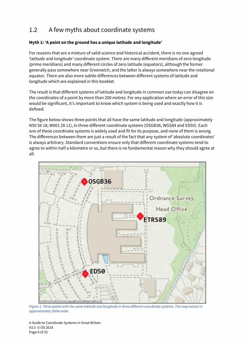
The figure below shows three points that all have the same latitude and longitude (approximately
N50 56 18, W001 28 11), in three different coordinate systems (OSGB36, WGS84 and ED50). Each
one of these coordinate systems is widely used and fit for its purpose, and none of them is wrong.
The differences between them are just a result of the fact that any system of ‘absolute coordinates’
is always arbitrary. Standard conventions ensure only that different coordinate systems tend to
agree to within half a kilometre or so, but there is no fundamental reason why they should agree at
all.
Figure 1. Three points with the same latitude and longitude in three different coordinate systems. The map extract is approximately 300m wide.
A Guide to Coordinate Systems in Great Britain
V3.3 © OS 2018
Page 7 of 53
Myth 2: ‘A horizontal plane is a level surface’
Of course it cannot be, because the Earth is round – any gravitationally level surface (such as the
surface of the wine in your glass, or the surface of the sea averaged over time) must curve as the
Earth curves, so it cannot be flat (that is, it cannot be a geometrical plane). But more than this, a
level surface has a complex shape – it is not a simple curved surface like a sphere. When we say ‘a
level surface’ we mean a surface that is everywhere at right angles to the direction of gravity. The
direction of gravity is generally towards the centre of the Earth as you would expect, but it varies in
direction and magnitude from place to place in a complex way, even on a very local scale. These
variations, which are too small for us to notice without specialist measuring equipment, are due to
the irregular distribution of mass on the surface (hills and valleys) and also to the variable density
of the Earth beneath us. Therefore, all level surfaces are actually bumpy and complex.
This is very important to coordinate systems used to map the height of the ground, because the
idea of quantified ‘height’ implies that there is a level surface somewhere below us which has zero
height. Even statements about relative height imply extended level surfaces. When we casually say
‘Point A is higher than point B’, what we really mean is ‘The level surface passing through point A, if
extended, would pass above point B’ So to accurately quantify the height difference between A
and B, we would need to know the shape of the level surface passing through point A. In fact we
choose a general ‘reference level surface’ of zero height covering the whole country to which we
can refer all our measured heights. This reference level surface is not flat!
Myth 3: ‘The true coordinates of a ground point do not change’
They certainly do, due to the continuous deforming motions of the Earth. Relative to the centre of
the Earth, a point on the ground can move as much as a metre up and down every day just because
of the tidal influences of the sun and moon. The relative motion of two continents can be 10
centimetres a year, which is significant for mapping because it is constant year after year – after 50
years a region of the earth may have moved by 5 metres relative to a neighbouring continent. Many
other small effects can be observed – the sinking of Britain when the tide comes in over the
continental shelf (a few centimetres), the sinking of inland areas under a weather system ‘high’
(about 5 millimetres), and the rising of the land in response to the melting of the last Ice Age (about
2 millimetres per year in Scotland, up to 1 centimetre per year in Scandinavia). Generally, as the
size of the region of the Earth over which we want to use a single coordinate system increases, the
more these dynamic Earth effects are significant.
The modern trend is to use global coordinate systems even for local applications. Therefore, it is
important to realise that in a global coordinate system, the ground on which we stand is
constantly moving. This leads to subtleties in coordinate system definition and use.
Myth 4: ‘There are exact mathematical formulae to change between coordinate systems’
Exact formulae only apply in the realm of perfect geometry – not in the real world of coordinated
points on the ground. The ‘known coordinates’ of a point in one coordinate system are obtained
from a large number of observations that are averaged together using a whole raft of assumptions.
Both the observations and the assumptions are only ever approximately correct and can be of
dubious quality, particularly if the point was coordinated a long time ago. It will also have moved
since it was coordinated, due to subsidence, continental plate motion and other effects.
A Guide to Coordinate Systems in Great Britain
V3.3 © OS 2018
Page 8 of 53
The result is that the relationship between two coordinate systems at the present time must also
be observed on the ground, and this observation too is subject to error. Therefore, only
approximate models can ever exist to transform coordinates from one coordinate system to
another. The first question to answer realistically is ‘What accuracy do I really require?’ In general,
if the accuracy requirements are low (5 to 10 metres, say) then transforming a set of coordinates
from one coordinate system to another is simple and easy. If the accuracy requirements are higher
(anywhere from 1 centimetre to half a metre, say), a more involved transformation process will be
required. In both cases, the transformation procedure should have a stated accuracy level.
2 The shape of the Earth
2.1 The first geodetic question
When you look at all the topographic and oceanographic details, the Earth is a very irregular and
complex shape. If you want to map the positions of those details, you need a simpler model of the
basic shape of the Earth, sometimes called the ‘figure of the Earth’, on which the coordinate
system will be based. The details can then be added by determining their coordinates relative to
the simplified shape, to build up the full picture.
The science of geodesy, on which all mapping and navigation is based, aims firstly to determine
the shape and size of the simplified ‘figure of the Earth’ and goes on to determine the location of
the features of the Earth’s land surface – from tectonic plates, coastlines and mountain ranges
down to the control marks used for surveying and making maps. Hence geodesists provide the
fundamental ‘points of known coordinates’ that cartographers and navigators take as their
starting point. The first question of geodesy, then, is ‘What is the best basic, simplified shape of the
Earth?’ Having established this, we can use it as a reference surface, with respect to which we
measure the topography.
Geodesists have two very useful answers to this question: ellipsoids and the Geoid. To really
understand coordinate systems, you need to understand these concepts first.
2.2 Ellipsoids
The Earth is very nearly spherical. However, it has a tiny equatorial bulge making the radius at the
equator about one third of one percent bigger than the radius at the poles. Therefore, the simple
geometric shape which most closely approximates the shape of the Earth is a biaxial ellipsoid,
which is the three-dimensional figure generated by rotating an ellipse about its shorter axis (less
exactly, it is the shape obtained by squashing a sphere slightly along one axis). The shorter axis of
the ellipsoid approximately coincides with the rotation axis of the Earth.
A Guide to Coordinate Systems in Great Britain
V3.3 © OS 2018
Page 9 of 53
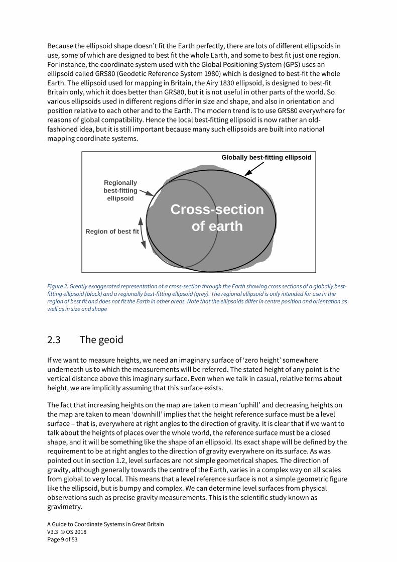
Because the ellipsoid shape doesn’t fit the Earth perfectly, there are lots of different ellipsoids in
use, some of which are designed to best fit the whole Earth, and some to best fit just one region.
For instance, the coordinate system used with the Global Positioning System (GPS) uses an
ellipsoid called GRS80 (Geodetic Reference System 1980) which is designed to best-fit the whole
Earth. The ellipsoid used for mapping in Britain, the Airy 1830 ellipsoid, is designed to best-fit
Britain only, which it does better than GRS80, but it is not useful in other parts of the world. So
various ellipsoids used in different regions differ in size and shape, and also in orientation and
position relative to each other and to the Earth. The modern trend is to use GRS80 everywhere for
reasons of global compatibility. Hence the local best-fitting ellipsoid is now rather an old-
fashioned idea, but it is still important because many such ellipsoids are built into national
mapping coordinate systems.
Figure 2. Greatly exaggerated representation of a cross-section through the Earth showing cross sections of a globally best-fitting ellipsoid (black) and a regionally best-fitting ellipsoid (grey). The regional ellipsoid is only intended for use in the region of best fit and does not fit the Earth in other areas. Note that the ellipsoids differ in centre position and orientation as well as in size and shape
2.3 The geoid
If we want to measure heights, we need an imaginary surface of ‘zero height’ somewhere
underneath us to which the measurements will be referred. The stated height of any point is the
vertical distance above this imaginary surface. Even when we talk in casual, relative terms about
height, we are implicitly assuming that this surface exists.
The fact that increasing heights on the map are taken to mean ‘uphill’ and decreasing heights on
the map are taken to mean ‘downhill’ implies that the height reference surface must be a level
surface – that is, everywhere at right angles to the direction of gravity. It is clear that if we want to
talk about the heights of places over the whole world, the reference surface must be a closed
shape, and it will be something like the shape of an ellipsoid. Its exact shape will be defined by the
requirement to be at right angles to the direction of gravity everywhere on its surface. As was
pointed out in section 1.2, level surfaces are not simple geometrical shapes. The direction of
gravity, although generally towards the centre of the Earth, varies in a complex way on all scales
from global to very local. This means that a level reference surface is not a simple geometric figure
like the ellipsoid, but is bumpy and complex. We can determine level surfaces from physical
observations such as precise gravity measurements. This is the scientific study known as
gravimetry.
Region of best fit
Globally best-fitting ellipsoid
Regionallybest-fitting
ellipsoid
Cross-sectionof earth
A Guide to Coordinate Systems in Great Britain
V3.3 © OS 2018
Page 10 of 53
Depending on what height we choose as ‘zero height’, there are any number of closed level
surfaces we could choose as our global height reference surface, and the choice is essentially
arbitrary. We can think of these level surfaces like layers of an onion inside and outside the Earth’s
topographic surface. Each one corresponds to a different potential energy level of the Earth’s
gravitational field, and each one, although an irregular shape, is a surface of constant height. The
one we choose as our height reference surface is that level surface which is closest to the average
surface of all the world’s oceans. This is a sensible choice since we are coastal creatures and we
like to think of sea level as having a height of zero. We call this irregular three-dimensional shape
the Geoid. Although it is both imaginary and difficult to measure, it is a single unique surface: it is
the only level surface which best fits the average surface of the oceans over the whole Earth. This is
by contrast with ellipsoids, of which there are many fitting different regions of the Earth.
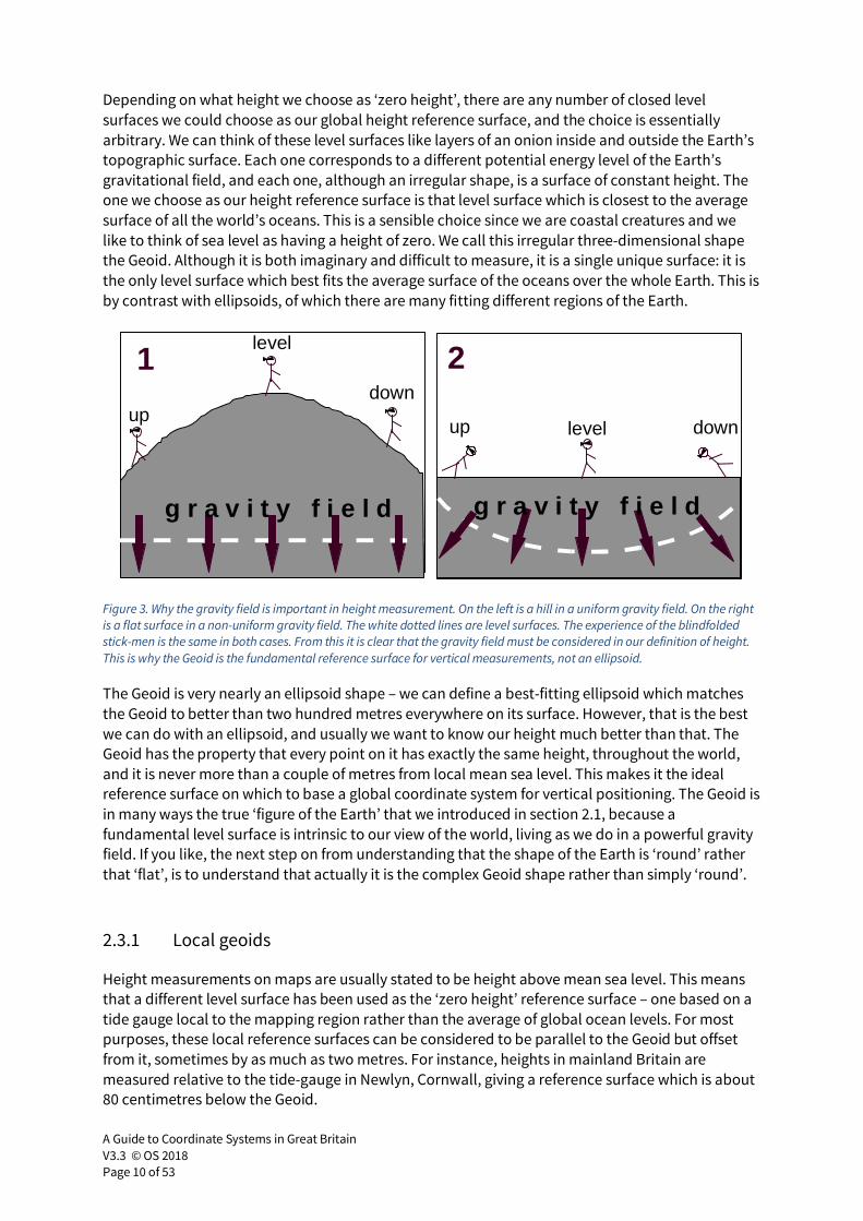
Figure 3. Why the gravity field is important in height measurement. On the left is a hill in a uniform gravity field. On the right is a flat surface in a non-uniform gravity field. The white dotted lines are level surfaces. The experience of the blindfolded stick-men is the same in both cases. From this it is clear that the gravity field must be considered in our definition of height. This is why the Geoid is the fundamental reference surface for vertical measurements, not an ellipsoid.
The Geoid is very nearly an ellipsoid shape – we can define a best-fitting ellipsoid which matches
the Geoid to better than two hundred metres everywhere on its surface. However, that is the best
we can do with an ellipsoid, and usually we want to know our height much better than that. The
Geoid has the property that every point on it has exactly the same height, throughout the world,
and it is never more than a couple of metres from local mean sea level. This makes it the ideal
reference surface on which to base a global coordinate system for vertical positioning. The Geoid is
in many ways the true ‘figure of the Earth’ that we introduced in section 2.1, because a
fundamental level surface is intrinsic to our view of the world, living as we do in a powerful gravity
field. If you like, the next step on from understanding that the shape of the Earth is ‘round’ rather
that ‘flat’, is to understand that actually it is the complex Geoid shape rather than simply ‘round’.
2.3.1 Local geoids
Height measurements on maps are usually stated to be height above mean sea level. This means
that a different level surface has been used as the ‘zero height’ reference surface – one based on a
tide gauge local to the mapping region rather than the average of global ocean levels. For most
purposes, these local reference surfaces can be considered to be parallel to the Geoid but offset
from it, sometimes by as much as two metres. For instance, heights in mainland Britain are
measured relative to the tide-gauge in Newlyn, Cornwall, giving a reference surface which is about
80 centimetres below the Geoid.
1 2
g r a v i t y f i e l dg r a v i t y f i e l d
up
level
down
up level down
A Guide to Coordinate Systems in Great Britain
V3.3 © OS 2018
Page 11 of 53
What causes this discrepancy between average global ocean levels and local mean sea levels? We
know that pure water left undisturbed does form a level surface, so the two should be in
agreement. The problem is that the sea around our coasts is definitely not left undisturbed! The
oceanic currents, effects of tides and winds on the coast, and variations in water temperature and
purity all cause ‘mean sea level’ to deviate slightly from the truly level Geoid surface. So, the mean
sea level surface contains very shallow hills and valleys which are described by the apt term ‘sea
surface topography’. The sea around Britain happens to form a ‘valley’ in the sea surface, so our
mean sea level is about 80 centimetres below the Geoid. Different countries have adopted different
local mean sea levels as their ‘zero height’ definition. Consequently, there are many ‘zero height’
reference surfaces used in different parts of the world which are (almost) parallel to, but offset
from, the true global Geoid. These reference surfaces are sometimes called ‘local geoids’ – the
capital G can be omitted in this case.
3 What is position
We have introduced an irregular, dynamic Earth and the concepts of ellipsoid and Geoid that are
used to describe its basic shape. Now we want to describe with certainty where we are on that
Earth, or where any feature is, in a simple numerical way. So, the challenge is to define a
coordinate system with which we can uniquely and accurately state the position of any
topographic feature as an unambiguous set of numbers. In the fields of geodesy, mapping and
navigation, a ‘position’ means a set of coordinates in a clearly defined coordinate system, along
with a statement of the likely error in those coordinates. How do we obtain this?
The answer to this question is the subject of the whole of this section. In section 3.1, we review the
different types of coordinates we commonly need to work with. In sections 3.2 and 3.3 we will look
at the two essential concepts in creating a terrestrial coordinate system that gives us a detailed
insight into what a set of coordinates (a geodetic position) really tells us.
3.1 Types of coordinates
3.1.1 Latitude, longitude and ellipsoid height
The most common way of stating terrestrial position is with two angles, latitude and longitude.
These define a point on the globe. More correctly, they define a point on the surface of an ellipsoid
that approximately fits the globe. Therefore, to use latitudes and longitudes with any degree of
certainty, you must know which ellipsoid you are dealing with.
A Guide to Coordinate Systems in Great Britain
V3.3 © OS 2018
Page 12 of 53
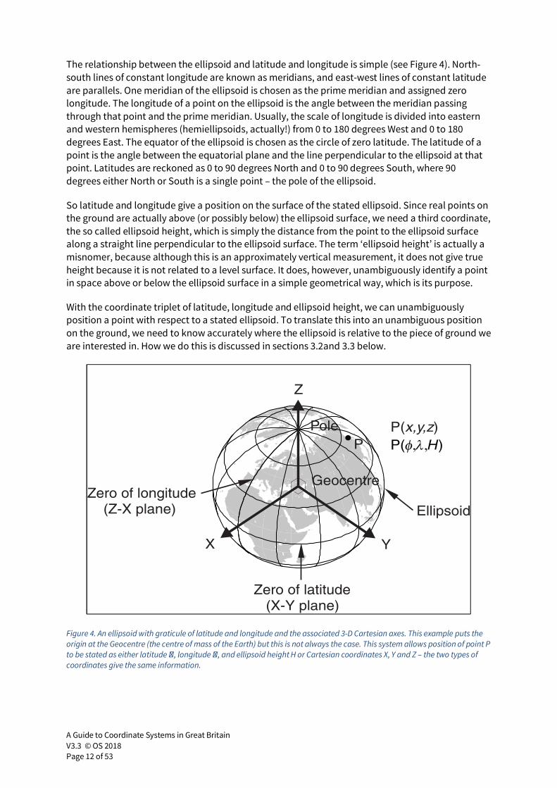
The relationship between the ellipsoid and latitude and longitude is simple (see Figure 4). North-
south lines of constant longitude are known as meridians, and east-west lines of constant latitude
are parallels. One meridian of the ellipsoid is chosen as the prime meridian and assigned zero
longitude. The longitude of a point on the ellipsoid is the angle between the meridian passing
through that point and the prime meridian. Usually, the scale of longitude is divided into eastern
and western hemispheres (hemiellipsoids, actually!) from 0 to 180 degrees West and 0 to 180
degrees East. The equator of the ellipsoid is chosen as the circle of zero latitude. The latitude of a
point is the angle between the equatorial plane and the line perpendicular to the ellipsoid at that
point. Latitudes are reckoned as 0 to 90 degrees North and 0 to 90 degrees South, where 90
degrees either North or South is a single point – the pole of the ellipsoid.
So latitude and longitude give a position on the surface of the stated ellipsoid. Since real points on
the ground are actually above (or possibly below) the ellipsoid surface, we need a third coordinate,
the so called ellipsoid height, which is simply the distance from the point to the ellipsoid surface
along a straight line perpendicular to the ellipsoid surface. The term ‘ellipsoid height’ is actually a
misnomer, because although this is an approximately vertical measurement, it does not give true
height because it is not related to a level surface. It does, however, unambiguously identify a point
in space above or below the ellipsoid surface in a simple geometrical way, which is its purpose.
With the coordinate triplet of latitude, longitude and ellipsoid height, we can unambiguously
position a point with respect to a stated ellipsoid. To translate this into an unambiguous position
on the ground, we need to know accurately where the ellipsoid is relative to the piece of ground we
are interested in. How we do this is discussed in sections 3.2and 3.3 below.
Figure 4. An ellipsoid with graticule of latitude and longitude and the associated 3-D Cartesian axes. This example puts the origin at the Geocentre (the centre of mass of the Earth) but this is not always the case. This system allows position of point P to be stated as either latitude , longitude , and ellipsoid height H or Cartesian coordinates X, Y and Z – the two types of coordinates give the same information.
A Guide to Coordinate Systems in Great Britain
V3.3 © OS 2018
Page 13 of 53
3.1.2 Cartesian coordinates
Rectangular Cartesian coordinates are a very simple system of describing position in three
dimensions, using three perpendicular axes X, Y and Z. Three coordinates unambiguously locate
any point in this system. We can use it as a very useful alternative to latitude, longitude and
ellipsoid height to convey exactly the same information.
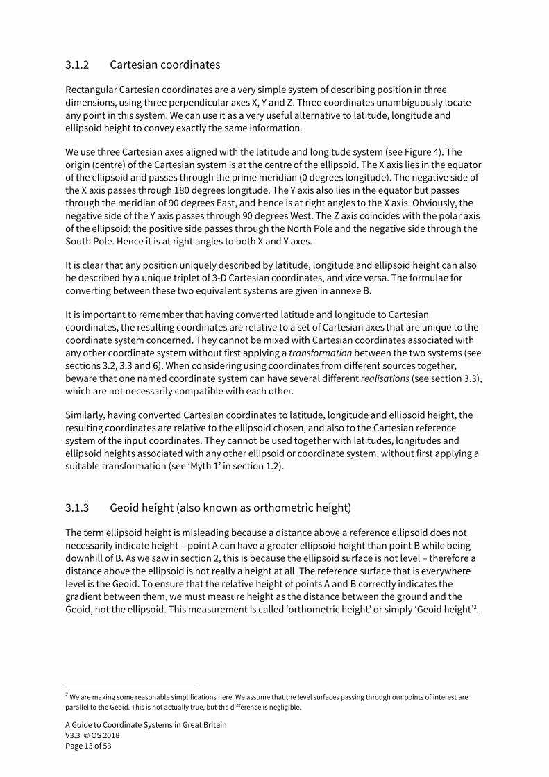
We use three Cartesian axes aligned with the latitude and longitude system (see Figure 4). The
origin (centre) of the Cartesian system is at the centre of the ellipsoid. The X axis lies in the equator
of the ellipsoid and passes through the prime meridian (0 degrees longitude). The negative side of
the X axis passes through 180 degrees longitude. The Y axis also lies in the equator but passes
through the meridian of 90 degrees East, and hence is at right angles to the X axis. Obviously, the
negative side of the Y axis passes through 90 degrees West. The Z axis coincides with the polar axis
of the ellipsoid; the positive side passes through the North Pole and the negative side through the
South Pole. Hence it is at right angles to both X and Y axes.
It is clear that any position uniquely described by latitude, longitude and ellipsoid height can also
be described by a unique triplet of 3-D Cartesian coordinates, and vice versa. The formulae for
converting between these two equivalent systems are given in annexe B.
It is important to remember that having converted latitude and longitude to Cartesian
coordinates, the resulting coordinates are relative to a set of Cartesian axes that are unique to the
coordinate system concerned. They cannot be mixed with Cartesian coordinates associated with
any other coordinate system without first applying a transformation between the two systems (see
sections 3.2, 3.3 and 6). When considering using coordinates from different sources together,
beware that one named coordinate system can have several different realisations (see section 3.3),
which are not necessarily compatible with each other.
Similarly, having converted Cartesian coordinates to latitude, longitude and ellipsoid height, the
resulting coordinates are relative to the ellipsoid chosen, and also to the Cartesian reference
system of the input coordinates. They cannot be used together with latitudes, longitudes and
ellipsoid heights associated with any other ellipsoid or coordinate system, without first applying a
suitable transformation (see ‘Myth 1’ in section 1.2).
3.1.3 Geoid height (also known as orthometric height)
The term ellipsoid height is misleading because a distance above a reference ellipsoid does not
necessarily indicate height – point A can have a greater ellipsoid height than point B while being
downhill of B. As we saw in section 2, this is because the ellipsoid surface is not level – therefore a
distance above the ellipsoid is not really a height at all. The reference surface that is everywhere
level is the Geoid. To ensure that the relative height of points A and B correctly indicates the
gradient between them, we must measure height as the distance between the ground and the
Geoid, not the ellipsoid. This measurement is called ‘orthometric height’ or simply ‘Geoid height’2.
2 We are making some reasonable simplifications here. We assume that the level surfaces passing through our points of interest are
parallel to the Geoid. This is not actually true, but the difference is negligible.
A Guide to Coordinate Systems in Great Britain
V3.3 © OS 2018
Page 14 of 53
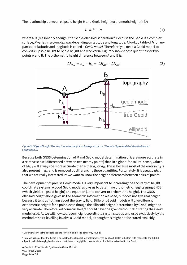
The relationship between ellipsoid height H and Geoid height (orthometric height) h is3:
� = ℎ +� �1�
where N is (reasonably enough) the ‘Geoid-ellipsoid separation’4. Because the Geoid is a complex
surface, N varies in a complex way depending on latitude and longitude. A lookup table of N for any
particular latitude and longitude is called a Geoid model. Therefore, you need a Geoid model to
convert ellipsoid height to Geoid height and vice-versa. Figure 5 shows these quantities for two
points A and B. The orthometric height difference between A and B is:
∆ℎ� = ℎ� − ℎ =∆�� − ∆�� �2�
Figure 5. Ellipsoid height H and orthometric height h of two points A and B related by a model of Geoid-ellipsoid separation N.
Because both GNSS determination of H and Geoid model determination of N are more accurate in
a relative sense (differenced between two nearby points) than in a global ‘absolute’ sense, values
of ∆ℎ� will always be more accurate than either ℎ or ℎ�. This is because most of the error in ℎ is
also present in ℎ� and is removed by differencing these quantities. Fortunately, it is usually ∆ℎ�
that we are really interested in: we want to know the height differences between pairs of points.
The development of precise Geoid models is very important to increasing the accuracy of height
coordinate systems. A good Geoid model allows us to determine orthometric heights using GNSS
(which yields ellipsoid height) and equation (1) (to convert to orthometric height). The GNSS
ellipsoid height alone gives us the geometric information we need, but does not give real height
because it tells us nothing about the gravity field. Different Geoid models will give different
orthometric heights for a point, even though the ellipsoid height (determined by GNSS) might be
very accurate. Therefore, orthometric height should never be given without also stating the Geoid
model used. As we will now see, even height coordinate systems set up and used exclusively by the
method of spirit levelling involve a Geoid model, although this might not be stated explicitly.
3 Unfortunately, some authors use the letters h and H the other way round!
4 Here we assume that the Geoid is parallel to the ellipsoid (actually it diverges by about 0.002° in Britain with respect to the GRS80
ellipsoid, which is negligible here) and that there is negligible curvature in a plumb-line extended to the Geoid.
ellipsoid
true Geoid
geoid model
topography
hA
NA
hB
NB
A
B
HAHB
A Guide to Coordinate Systems in Great Britain
V3.3 © OS 2018
Page 15 of 53
3.1.4 Mean sea level height
We will now take a look at the Geoid model used in OS mapping on the British mainland, although
most surveyors might not immediately think of it as such. This is the Ordnance Datum Newlyn
(ODN) vertical coordinate system. Ordnance Survey maps state that heights are given above ‘mean
sea level’. If we’re looking for sub-metre accuracy in heighting this is a vague statement, since
mean sea level (MSL) varies over time and from place to place, as we noted in section 2.3.
ODN corresponds to the average sea level measured by the tide-gauge at Newlyn, Cornwall
between 1915 and 1921. Heights that refer to this particular MSL as the point of zero height are
called ODN heights. ODN is therefore a ‘local geoid’ definition as discussed in section 2.3. ODN
heights are used for all British mainland Ordnance Survey contours, spot heights and bench mark
heights. ODN heights are unavailable on many offshore islands, which have their own MSL based
on a local tide-gauge.
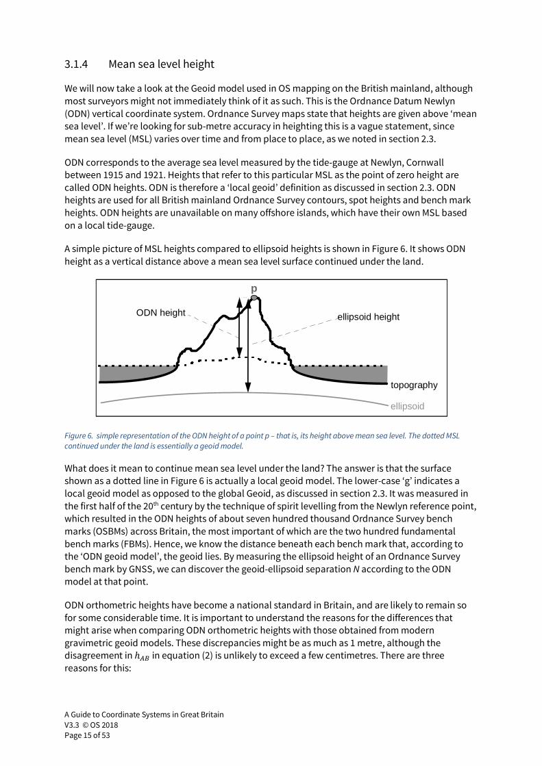
A simple picture of MSL heights compared to ellipsoid heights is shown in Figure 6. It shows ODN
height as a vertical distance above a mean sea level surface continued under the land.
Figure 6. simple representation of the ODN height of a point p – that is, its height above mean sea level. The dotted MSL continued under the land is essentially a geoid model.
What does it mean to continue mean sea level under the land? The answer is that the surface
shown as a dotted line in Figure 6 is actually a local geoid model. The lower-case ‘g’ indicates a
local geoid model as opposed to the global Geoid, as discussed in section 2.3. It was measured in
the first half of the 20th century by the technique of spirit levelling from the Newlyn reference point,
which resulted in the ODN heights of about seven hundred thousand Ordnance Survey bench
marks (OSBMs) across Britain, the most important of which are the two hundred fundamental
bench marks (FBMs). Hence, we know the distance beneath each bench mark that, according to
the ‘ODN geoid model’, the geoid lies. By measuring the ellipsoid height of an Ordnance Survey
bench mark by GNSS, we can discover the geoid-ellipsoid separation N according to the ODN
model at that point.
ODN orthometric heights have become a national standard in Britain, and are likely to remain so
for some considerable time. It is important to understand the reasons for the differences that
might arise when comparing ODN orthometric heights with those obtained from modern
gravimetric geoid models. These discrepancies might be as much as 1 metre, although the
disagreement in ℎ� in equation (2) is unlikely to exceed a few centimetres. There are three
reasons for this:
p
ODN height
topography
ellipsoid
ellipsoid height
A Guide to Coordinate Systems in Great Britain
V3.3 © OS 2018
Page 16 of 53
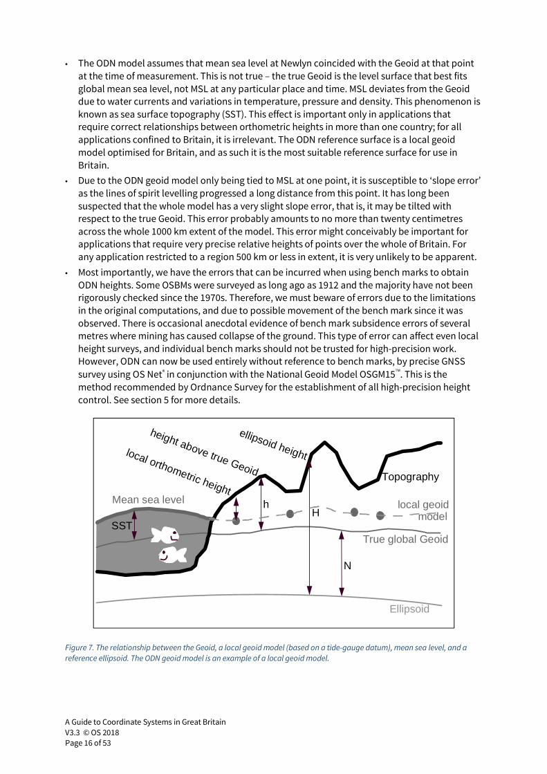
• The ODN model assumes that mean sea level at Newlyn coincided with the Geoid at that point
at the time of measurement. This is not true – the true Geoid is the level surface that best fits
global mean sea level, not MSL at any particular place and time. MSL deviates from the Geoid
due to water currents and variations in temperature, pressure and density. This phenomenon is
known as sea surface topography (SST). This effect is important only in applications that
require correct relationships between orthometric heights in more than one country; for all
applications confined to Britain, it is irrelevant. The ODN reference surface is a local geoid
model optimised for Britain, and as such it is the most suitable reference surface for use in
Britain.
• Due to the ODN geoid model only being tied to MSL at one point, it is susceptible to ‘slope error’
as the lines of spirit levelling progressed a long distance from this point. It has long been
suspected that the whole model has a very slight slope error, that is, it may be tilted with
respect to the true Geoid. This error probably amounts to no more than twenty centimetres
across the whole 1000 km extent of the model. This error might conceivably be important for
applications that require very precise relative heights of points over the whole of Britain. For
any application restricted to a region 500 km or less in extent, it is very unlikely to be apparent.
• Most importantly, we have the errors that can be incurred when using bench marks to obtain
ODN heights. Some OSBMs were surveyed as long ago as 1912 and the majority have not been
rigorously checked since the 1970s. Therefore, we must beware of errors due to the limitations
in the original computations, and due to possible movement of the bench mark since it was
observed. There is occasional anecdotal evidence of bench mark subsidence errors of several
metres where mining has caused collapse of the ground. This type of error can affect even local
height surveys, and individual bench marks should not be trusted for high-precision work.
However, ODN can now be used entirely without reference to bench marks, by precise GNSS
survey using OS Net® in conjunction with the National Geoid Model OSGM15. This is the
method recommended by Ordnance Survey for the establishment of all high-precision height
control. See section 5 for more details.
Figure 7. The relationship between the Geoid, a local geoid model (based on a tide-gauge datum), mean sea level, and a reference ellipsoid. The ODN geoid model is an example of a local geoid model.
ellipsoid height
Ellipsoid
True global Geoid
local geoid
Topography
Mean sea level
local orthometric height
SST
height above true Geoid
model
N
Hh
A Guide to Coordinate Systems in Great Britain
V3.3 © OS 2018
Page 17 of 53
3.1.5 Eastings and northings
The last type of coordinates we need to consider is eastings and northings, also called plane
coordinates, grid coordinates or map coordinates. These coordinates are used to locate position
with respect to a map, which is a two-dimensional plane surface depicting features on the curved
surface of the Earth. These days, the ‘map’ might be a computerised geographical information
system (GIS) but the principle is exactly the same. Map coordinates use a simple 2-D Cartesian
system, in which the two axes are known as eastings and northings. Map coordinates of a point are
computed from its ellipsoidal latitude and longitude by standard formulae known collectively as a
map projection. This is the coordinate type most often associated with the Ordnance Survey
National Grid.
A map projection cannot be a perfect representation, because it is not possible to show a curved
surface on a flat map without creating distortions and discontinuities. Therefore, different map
projections are used for different applications. The map projections commonly used in Britain are
the Ordnance Survey National Grid projection, and the Universal Transverse Mercator projection.
These are both projections of the Transverse Mercator type. Any coordinates stated as eastings
and northings should be accompanied by an exact statement of the map projection used to create
them. The formulae for the Transverse Mercator projection are given in annex C and the
parameters used in Britain are in annex A. There is more about map projections and the National
Grid in section 7.
In geodesy, map coordinates tend only to be used for visual display purposes. When we need to do
computations with coordinates, we use latitude and longitude or Cartesian coordinates, then
convert the results to map coordinates as a final step if needed. This working procedure is in
contrast to the practice in geographical information systems, where map coordinates are used
directly for many computational tasks. The Ordnance Survey transformation between the GNSS
coordinate system and the National Grid works directly with map coordinates – more about this in
section 6.3.
3.2 We need a datum
We have come some way in answering the question ‘What is position?’ by introducing various
types of coordinates: we use one or more of these coordinate types to state the positions of points
and features on the surface of the Earth.
No matter what type of coordinates we are using, we will require a suitable origin with respect to
which the coordinates are stated. For instance, we cannot use Cartesian coordinates unless we
have defined an origin point of the coordinate axes and defined the directions of the axes in
relation to the Earth we are measuring. This is an example of a set of conventions necessary to
define the spatial relationship of the coordinate system to the Earth. The general name for this
concept is the Terrestrial Reference System (TRS) or geodetic datum5. Datum is the most familiar
term amongst surveyors, and we will use it throughout this booklet. TRS is a more modern term for
the same thing.
To use 3-D Cartesian coordinates, a 3-D datum definition is required, in order to set up the three
5 This term is often misused. The term datum refers only to the arbitrarily chosen elements of a coordinate system necessary to define
the origin of coordinates – not to any control network based on this.
A Guide to Coordinate Systems in Great Britain
V3.3 © OS 2018
Page 18 of 53
axes, X, Y and Z. The datum definition must somehow state where the origin point of the three axes
lies and in what directions the axes point, all in relation to the surface of the Earth. Each point on
the Earth will then have a unique set of Cartesian coordinates in the new coordinate system. The
datum definition is the link between the ‘abstract’ coordinates and the real physical world.
To use latitude, longitude and ellipsoid height coordinates, we start with the same type of datum
used for 3-D Cartesian coordinates. To this, we add a reference ellipsoid centred on the Cartesian
origin (as in Figure 4), the shape and size of which is added to the datum definition. The size is
usually defined by stating the distance from the origin to the ellipsoid equator, which is called the
semi-major axis a. The shape is defined by any one of several parameters: the semi-minor axis
length b (the distance from the origin to the ellipsoid pole), the squared eccentricity e>, or the
inverse flattening . Exactly what these parameters represent is not important here. Each
conveys the same information: the shape of the chosen reference ellipsoid.
The term geodetic datum is usually taken to mean the ellipsoidal type of datum just described: a
set of 3-D Cartesian axes plus an ellipsoid, which allows positions to be equivalently described in 3-
D Cartesian coordinates or as latitude, longitude and ellipsoid height. This type of datum is
illustrated in figure 4. The datum definition consists of eight parameters: the 3-D location of the
origin (three parameters), the 3-D orientation of the axes (three parameters), the size of the
ellipsoid (one parameter) and the shape of the ellipsoid (one parameter).
There are, however, other types of geodetic datum. For instance, a local datum for orthometric
height measurement is very simple: it consists of the stated height of a single fundamental bench
mark. (NOTE: modern height datums are becoming more and more integrated with ellipsoidal datums through the use of Geoid models. The ideal is a single datum definition for horizontal and vertical measurements.)
What all datums have in common is that they are specified a priori – they are in essence, arbitrary
conventions, although they will be chosen to make things as easy as possible for users and to
make sense in the physical world. Because the datum is just a convention, a set of coordinates can
in theory be transformed from one datum to another and back again exactly. In practice, this
might not be very useful, as we shall see in sections 3.3 and 6.1.
3.2.1 Datum definition before the space age
How do we specify the position and orientation of a set of Cartesian axes in relation to the ground,
when the origin of the axes, and the surface of the associated ellipsoid, are within the Earth? The
way it used to be done before the days of satellite positioning was to use a particular ground mark
as the initial point of the coordinate system. This ground mark is assigned coordinates that are
essentially arbitrary, but fit for the purpose of the coordinate system.
Also, the direction towards the origin of the Cartesian axes from that point was chosen. This was
expressed as the difference between the direction of gravity at that point and the direction
towards the origin of the coordinate system. Because that is a three-dimensional direction, three
parameters were required to define it. So, we have six conventional parameters of the initial point
in all, which correspond to choosing the centre (in three dimensions) and the orientation (in three
dimensions) of the Cartesian axes. To enable us to use the latitude, longitude and ellipsoid height
coordinate type, we also choose the ellipsoid shape and size, which are a further two parameters.
Once the initial point is assigned arbitrary parameters in this way, we have defined a coordinate
f1
A Guide to Coordinate Systems in Great Britain
V3.3 © OS 2018
Page 19 of 53
system in which all other points on the Earth have unique coordinates – we just need a way to
measure them! We will look at the principles of doing this in the next section.
Although it is a good example of defining a datum, these days, a single initial point would never be
used for this purpose. Instead, we define the datum ‘implicitly’ by applying certain conditions to
the computed coordinates of a whole set of points, no one of which has special importance. This
method has become common in global GNSS coordinate systems since the 1980s. Avoiding
reliance on a single point gives practical robustness to the datum definition and makes error
analysis more straightforward.
3.3 Realising the datum definition with a Terrestrial Reference
Frame
With our datum definition we have located the origin, axes and ellipsoid of the coordinate system
with respect to the Earth’s surface, on which are the features we want to measure and describe.
We now come to the problem of making that coordinate system available for use in practice. If the
coordinate system is going to be used consistently over a large area, this is a big task. It involves
setting up some infrastructure of points to which users can have access, the coordinates of which
are known at the time of measurement. These reference points are typically either on the ground,
or on satellites orbiting the Earth. All positioning methods rely on line-of-sight from an observing
instrument to reference points of known coordinates. Putting some of the reference points on
orbiting satellites has the advantage that any one satellite is visible to a large area of the Earth’s
surface at any one time. This is the idea of satellite positioning.
The network of reference points with known coordinates is called the coordinate Terrestrial Reference Frame (TRF), and its purpose is to realise the coordinate system by providing accessible
points of known coordinates. Examples of TRFs are the network of Ordnance Survey triangulation
pillars seen on hilltops across Britain, and the constellation of 24 GPS satellites operated by the
United States Department of Defense. Both these TRFs serve exactly the same purpose: they are
highly visible points of known position in particular coordinate systems (in the case of satellites,
the points move so the ‘known position’ changes as a function of time). Users can observe these
TRF points using a positioning tool (a theodolite or a GNSS receiver in these examples) and hence
obtain new positions of previously unknown points in the coordinate system.
A vital conceptual difference between a datum and a TRF is that the former is errorless while the
latter is subject to error. A datum might be unsuitable for a certain application, but it cannot
contain errors because it is simply a set of conventionally adopted parameters – they are correct
by definition! A TRF, on the other hand, involves the physical observation of the coordinates of
many points – and wherever physical observations are involved, errors are inevitably introduced.
Therefore it is quite wrong to talk of errors in a datum: the errors occur in the realisation of that
datum by a TRF to make it accessible to users.
Most land surveyors do not speak of TRFs – instead we often misuse the term ‘datum’ to cover
both. This leads to a lot of misunderstandings, especially when comparing the discrepancies
between two coordinate systems. To understand the relationship between two coordinate
systems properly, we need to understand that the difference in their datums can be given by some
exact set of parameters, although we might not know what they are. On the other hand, the
difference in their TRFs (which is what we generally really want to know) can only be described in
approximate terms, with a statistical accuracy statement attached to the description.
A Guide to Coordinate Systems in Great Britain
V3.3 © OS 2018
Page 20 of 53
In sections 4 and 5 below, we look at real geodetic coordinate systems in terms of their datums
and TRFs in some detail. These case studies provide some examples to illustrate the concepts
introduced here.
3.4 Summary
With the three concepts summarised in table, we can set up and use a coordinate system.
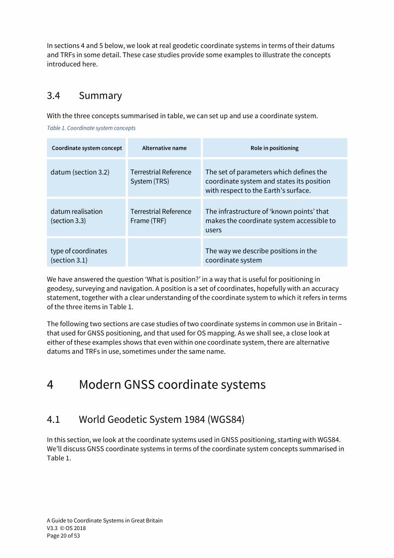
Table 1. Coordinate system concepts
Coordinate system concept Alternative name Role in positioning
datum (section 3.2) Terrestrial Reference
System (TRS)
The set of parameters which defines the
coordinate system and states its position
with respect to the Earth’s surface.
datum realisation
(section 3.3)
Terrestrial Reference
Frame (TRF)
The infrastructure of ‘known points’ that
makes the coordinate system accessible to
users
type of coordinates
(section 3.1)
The way we describe positions in the
coordinate system
We have answered the question ‘What is position?’ in a way that is useful for positioning in
geodesy, surveying and navigation. A position is a set of coordinates, hopefully with an accuracy
statement, together with a clear understanding of the coordinate system to which it refers in terms
of the three items in Table 1.
The following two sections are case studies of two coordinate systems in common use in Britain –
that used for GNSS positioning, and that used for OS mapping. As we shall see, a close look at
either of these examples shows that even within one coordinate system, there are alternative
datums and TRFs in use, sometimes under the same name.
4 Modern GNSS coordinate systems
4.1 World Geodetic System 1984 (WGS84)
In this section, we look at the coordinate systems used in GNSS positioning, starting with WGS84.
We’ll discuss GNSS coordinate systems in terms of the coordinate system concepts summarised in
Table 1.
A Guide to Coordinate Systems in Great Britain
V3.3 © OS 2018
Page 21 of 53
The datum used for GPS positioning is called WGS84 (World Geodetic System 1984). It consists of a
three-dimensional Cartesian coordinate system and an associated ellipsoid so that WGS84
positions can be described as either XYZ Cartesian coordinates or latitude, longitude and ellipsoid
height coordinates. The origin of the datum is the Geocentre (the centre of mass of the Earth) and
it is designed for positioning anywhere on Earth.
In line with the definition of a datum given in section 3.2 the WGS84 datum is nothing more than a
set of conventions, adopted constants and formulae. No physical infrastructure is included, and
the definition does not indicate how you might position yourself in this system. The WGS84
definition includes the following items:
• The WGS84 Cartesian axes and ellipsoid are geocentric; that is, their origin is the centre of mass
of the whole Earth including oceans and atmosphere.
• The scale of the axes is that of the local Earth frame, in the sense of the relativistic theory of
gravitation.
• Their orientation (that is, the directions of the axes, and hence the orientation of the ellipsoid
equator and prime meridian of zero longitude) coincided with the equator and prime meridian
of the Bureau Internationale de l’Heure at the moment in time 1984.0 (that is, midnight on New
Year’s Eve 1983).
• Since 1984.0, the orientation of the axes and ellipsoid has changed such that the average
motion of the crustal plates relative to the ellipsoid is zero. This ensures that the Z-axis of the
WGS84 datum coincides with the International Reference Pole, and that the prime meridian of
the ellipsoid (that is, the plane containing the Z and X Cartesian axes) coincides with the
International Reference Meridian.
• The shape and size of the WGS84 biaxial ellipsoid is defined by the semi-major axis length
a = 6378137.000 metres, and the reciprocal of flattening 1/f = 298.257223563. This ellipsoid is
very, very close in shape and size to the GRS80 ellipsoid.
• Conventional values are also adopted for the standard angular velocity of the Earth, and for the
Earth gravitational constant. The first is needed for time measurement, and the second to
define the scale of the system in a relativistic sense. We will not consider these parameters
further here.
There are a couple of points to note about this definition. Firstly, the ellipsoid is designed to
best-fit the Geoid of the Earth as a whole. This means it generally doesn’t fit the Geoid in a
particular country as well as the non-geocentric ellipsoid used for mapping that country. In Britain,
GRS80 lies about 50 metres below the Geoid and slopes from east to west relative to the Geoid, so
the Geoid-ellipsoid separation is 10 metres greater in the west than in the east. Our local mapping
ellipsoid (the Airy 1830 ellipsoid) is a much better fit.
Secondly, note that the axes of the WGS84 Cartesian system, and hence all lines of latitude and
longitude in the WGS84 datum, are not stationary with respect to any particular country. Due to
tectonic plate motion, different parts of the world move relative to each other with velocities of the
order of ten centimetres per year. The International Reference Meridian and Pole, and hence the
WGS84 datum, are stationary with respect to the average of all these motions. But this means they
are in motion relative to any particular region or country. In Britain, all WGS84 latitudes and
longitudes are changing at a constant rate of about 2.5 centimetres per year in a north-easterly
direction. Over the course of a decade or so, this effect becomes noticeable in large-scale
mapping. Some parts of the world (for example Hawaii and Australia) are moving at up to one
metre per decade relative to WGS84.
The full definition of WGS84 is available on the Internet – see section 8 for the address.
A Guide to Coordinate Systems in Great Britain
V3.3 © OS 2018
Page 22 of 53
4.2 Realising WGS84 with a TRF
So much for the theoretical definition of WGS84 – how can we use it? At first sight a coordinate
system centred on the centre of mass of the Earth, oceans and atmosphere might seem very
difficult to realise. Actually, this definition is very convenient for satellite positioning, because the
centre of mass of the Earth (often called the geocentre) is one of the foci of the elliptical orbits of
all Earth satellites6, assuming the mass of the satellite itself is negligible. Therefore, observing a
satellite can tell us, more or less, where the centre of the Earth is.
There are no fewer than three Terrestrial Reference Frames realising WGS84 that are very
important to us in Britain. They are: the United States military ‘broadcast’ realisation; the
International Terrestrial Reference Frame (ITRF) precise scientific realisation; and the European
Terrestrial Reference Frame (ETRF) Europe-fixed realisation. We will look at each in turn. We will
see that each of these actually realises a slightly different datum, although all of them are loosely
referred to as ‘WGS84 realisations’.
4.2.1 The WGS84 broadcast TRF
The primary means of navigating in the WGS84 coordinate system is via the WGS84 positions of the
GPS satellites, which are continuously broadcast by the satellites themselves. This satellite
constellation is a TRF – that is, it is a general-purpose access tool making the WGS84 coordinate
system available to users.
The WGS84 satellite positions are determined by the US Department of Defense using a network of
tracking stations, the positions of which have been precisely computed. The tracking stations
observe the satellites and hence determine the WGS84 coordinates of the satellites. The quality of
the resulting satellite coordinates depends on the quality of the known tracking station
coordinates. These were initially not very good (probably 10 metre accuracy) but have been
refined several times. The tracking station coordinates are now very close agreement with the
International Reference Meridian and International Reference Pole.
The network of GPS tracking stations can be considered the original WGS84 TRF. The satellite
constellation, which is a derived TRF, can be seen as a tool to transfer this realisation ‘over the
horizon’ to wherever positioning is needed in the world. The current coordinates of the tracking
station antennae implicitly state the physical origin, orientation and scale of the system – they
have been computed such that these elements are as close as possible to the theoretical
requirements listed in section 4.1. Of course, no TRF is perfect – this one is probably good to five
centimetres or so.
Prior to May 2000, the full accuracy of the US tracking station TRF was not made available to non-
military users. In the transfer of this TRF to satellite positions, positional accuracies were
deliberately worsened by a feature known as selective availability (SA). This meant that a civilian
user, with a single GPS receiver, could not determine WGS84 position to an accuracy better than
about 100 metres. In May 2000, this intentional degradation of the GPS signals was officially
switched off.
6 Orbiting satellites naturally move in ellipses, which have two focal points. The centre of mass of the earth-satellite system lies at one
focus of the ellipse. A circle is the special case of an ellipse where the two focal points coincide.
A Guide to Coordinate Systems in Great Britain
V3.3 © OS 2018
Page 23 of 53
With a pair of GNSS receivers we can accurately measure their relative positions (that is, the
three-dimensional vector between the two receivers can be accurately determined). We must put
one of these receivers on a known point and leave it there. This is known as relative GNSS
positioning or differential GNSS. Fortunately, there are methods of accurately determining the real
WGS84 position of the known point and hence recovering correct WGS84 positions, using the civil
GNSS TRFs which are the subject of the following sections.
4.2.2 The International Terrestrial Reference Frame (ITRF)
The ITRF is an alternative realisation of WGS84 that is produced by the International Earth
Rotation and Reference System Service (IERS) based in Paris, France. It includes many more
stations than the broadcast WGS84 TRF – more than 500 stations at 290 sites all over the world.
Four different space positioning methods contribute to the ITRF – Very Long Baseline
Interferometry (VLBI), Satellite Laser Ranging (SLR), Global Navigation Satellite Systems (GNSS)
and Doppler Ranging Integrated on Satellite (DORIS). Each has strengths and weaknesses – their
combination produces a strong multi-purpose TRF. ITRF was created by the civil GNSS community,
quite independently of the US military organisations that operate the broadcast TRF.
Each version of the ITRF is supplemented with a 4 digit year code to identify it – ITRFyyyy. Each
ITRFyyyy is simply a list of coordinates (X Y and Z in metres) and velocities (dX, dY and dZ in metres
per year) of each station in the TRF, together with the estimated level of error in those values. The
coordinates usually relate to the time yyyy.0 (i.e. 00:00 on 1st Jan of year yyyy). To obtain the
coordinates of a station at any other time, the station velocity is applied appropriately. This is to
cope with the effects of tectonic plate motion. Each ITRFyyyy is available as a SINEX format text file
from the IERS Internet website – see section 8 for the address.
The datum realised by the ITRF is actually called ITRS (International Terrestrial Reference System)
rather than WGS84. There used to be a difference between the two, but they have been
progressively brought together and are now so similar that they can be assumed identical for
almost all purposes. Because the ITRF is of higher quality than the military WGS84 TRF, the WGS84
datum now effectively takes its definition from ITRS. Therefore, although in principle the
broadcast TRF is the principal realisation of WGS84, in practice ITRF has become the more
important TRF because it has proven to be the most accurate global TRF ever constructed. The
defining conventions of ITRS are identical to those of WGS84 given in section 4.1.
The ITRF is important to us for two reasons. Firstly, we can use ITRF stations equipped with
permanent GNSS receivers as reference points of known coordinates to precisely coordinate our
own GNSS stations, using GNSS data downloaded from the Internet. This procedure is known as
‘fiducial GNSS analysis’. Secondly, we can obtain precise satellite positions (known as
ephemerides) in the current ITRF that are more accurate than the ephemerides transmitted by the
GNSS satellites. Both these vital geodetic services are provided free, via the Internet, by the
International GNSS Service.
4.2.3 The International GNSS Service (IGS)
The IGS is essential for anybody requiring high accuracy GNSS derived positions. The IGS operates
a global TRF of 505 GNSS stations (as of February 2018) and from these produces the following free
products, distributed via the Internet:
A Guide to Coordinate Systems in Great Britain
V3.3 © OS 2018
Page 24 of 53
• IGS tracking station dual-frequency GNSS data.
• Precise GNSS satellite orbits (ephemerides).
• GNSS satellite clock parameters.
• Earth orientation parameters.
• IGS tracking station coordinates and velocities; many of these stations are also listed in the
ITRF.
• Zenith path delay estimates.
Of these, the first two are commonly used for general-purpose high-accuracy positioning, and the
third is becoming increasingly important. The satellite ephemerides, clock parameters and Earth
rotation parameters are available two days after the time of observation, and also in advance of
the observation in a less accurate predicted version.
The IGS products give us access to a high-accuracy realisation based on the current ITRF. Used in
conjunction with the ITRF coordinates of nearby IGS tracking stations and the dual-frequency
GNSS data from those stations, a user can position a single geodetic-quality GNSS receiver to
within a few millimetres. Hence the IGS products are a vital part of the civil GNSS community’s
access to the ITRF.
Because the subject of this booklet is coordinate systems, not GNSS positioning methods, no more
will be said about IGS here. Please see the further information list in section 6 for more information
on precise GNSS positioning and the IGS web page address.
4.2.4 European Terrestrial Reference System 1989 (ETRS89)
With each of the three GNSS TRFs we have encountered so far (US DoD tracking stations, broadcast
GNSS orbits, and IERS/IGS TRF) a new version of the WGS84 datum has been introduced. Geodetic
datums are like this – in theory the datum is exactly specified by the adopted conventions (listed in
section 4.1) but in practice, each TRF intended to realise that specification actually implements a
slightly different datum. Often, there are deliberate reasons for this, as in the case of the deliberate
random element (Selective Availability) that was at one time introduced to the WGS84 datum in
the broadcast satellite orbits.
Another type of deliberate variation to the WGS84 datum definition is found in realisations that are
intended to serve a particular geographic region for mapping purposes. As we saw in listed in
section 4.1, the WGS84 position of any particular point on the Earth’s surface is changing
continuously due to various effects, the most important of which is tectonic motion. So WGS84
itself is unsuitable for mapping – the ground keeps sliding across the surface of any WGS84
mapping grid!
A Guide to Coordinate Systems in Great Britain
V3.3 © OS 2018
Page 25 of 53
However, it is still useful to have a mapping coordinate system that is compatible with GNSS. This
is done by selecting a particular moment in time (in geodesy a moment in time is called an epoch,
which is an unusual usage of that word), and stating the WGS84 coordinates of points in the region
of interest at that epoch, regardless of the time of observation. Remember that the Cartesian axes
and ellipsoid of WGS84 move steadily such that the motion is minimal with respect to the average
of tectonic plate motions worldwide. Fixing the datum epoch has the effect of creating a new
datum definition (that is, a new set of Cartesian axes and ellipsoid location and orientation) which
initially coincides exactly with WGS84, but from then on remains stationary with respect to the
particular piece of the Earth’s crust where the fixed points are, while moving steadily away from
the WGS84 axes and ellipsoid.
This adoption of a particular WGS84 epoch to remove the effect of tectonic motion has been done
in various places in the world – in fact, everywhere WGS84 has been adopted for mapping.
Examples of WGS84-like datums which are gradually diverging from WGS84 are North American
Datum 1983, New Zealand Geodetic Datum 2000, and the Geocentric Datum of Australia. There is
also a European example, the European Terrestrial Reference System 1989 (ETRS89), which as the
name suggests is a datum that coincided with WGS84 at the moment in time 1989.0, and has been
slowly diverging ever since, moving with the Eurasian land mass. ETRS89 is ideal for a Europe-wide
consistent mapping and data sets and it is mandatory for any data set complying with the EU
INSPIRE directive.
For every realisation of ITRS (e.g. ITRF97, ITRF2000, ITRF2005,…) there is an equivalent TRF
associated with ETRS89, called ETRFyyyy (or yy pre year 2000) where yyyy is the year of the
“parent” ITRF (e.g. ETRF97, ETRF2000, ETRF2005 and so on). However, the epoch of all the ETRFs is
1989.0 so they are closely aligned with each other. What can be confusing is that often the ETRF
will be quoted with an epoch relating to the parent ITRF from which it was derived. For example
the current realisation of the OS Net coordinates (see section 5.1) are of course in ETRS89 (epoch
1989.0) but the “official” designation would be ETRF97 epoch 2009.756. That is - the parent ITRF is
ITRF97 realised from observations centred on epoch 2009.756 (00:00:00, 04/10/2009). This
information regarding the “parent” ITRF is useful if transforming between an ETRF and other
ITRFs.
The reason for a new ETRF every time ITRF is updated is to take advantage of the improvements in
the ITRF realisation and also to keep the ETRS89 realisation as close as possible to the current ITRS
one, but still at epoch 1989.0.
Although not identical with WGS84, these locally-fixed GNSS datums are very easily and accurately
related back to WGS84. This is because tectonic plate motion is very steady, predictable and
precisely known. The ETRS89 coordinate of any point can easily be converted to a WGS84
coordinate via a simple transformation. See section 6.5.
The importance of ETRS89 and ETRF to us in Britain is that this is the datum and TRF used for all
OS GNSS positioning. It is a convenient system because we can forget about the tectonic effects
apparent in WGS84 (which do not concern us in British mapping), while still being able easily to
convert these coordinates to WGS84 when required. OS Net uses ETRS89 as its datum, and is a
densification of the ETRF. More about this in the next section.
A Guide to Coordinate Systems in Great Britain
V3.3 © OS 2018
Page 26 of 53
5 Ordnance Survey coordinate systems
Let’s now take a look at the coordinate systems used by OS for mapping Great Britain. There are
three coordinate systems to consider:
• OS Net, a modern 3-D TRF using the ETRS89 datum (as described in section 4.2.4). This
coordinate system is the basis of modern Ordnance Survey ‘control survey’ (the surveyor’s
jargon for adding local points to a TRF for mapping purposes), and is the basis of definition of
all Ordnance Survey coordinates. A subset of OS Net (see section 5.1) has been ratified as the
official densification of ETRF89 in GB.
• The National Grid, a ‘traditional’ horizontal coordinate system, which consists of: a traditional
geodetic datum (see section 3.2) using the Airy 1830 ellipsoid; a TRF called OSGB36
(Ordnance Survey Great Britain 1936) which was observed by theodolite triangulation of trig
pillars; and a Transverse Mercator map projection (see section 7 below) allowing the use of
easting and northing coordinates. This coordinate system is important because it is used to
describe the horizontal positions of features on British maps. However, its historical origins and
observation methods are not of interest to most users and will be skipped over in this booklet.
National Grid coordinates are nowadays determined by GNSS plus a transformation rather than
theodolite triangulation.
• Ordnance Datum Newlyn (ODN), a ‘traditional’ vertical coordinate system, consisting of a
tide-gauge datum with initial point at Newlyn (Cornwall), and a TRF observed by spirit levelling
between 200 fundamental bench marks (FBMs) across Britain. The TRF is densified by more
than half a million lower-accuracy bench marks. Each bench mark has an orthometric height
only (not ellipsoid height or accurate horizontal position). This coordinate system is important
because it is used to describe vertical positions of features on British maps (for example, spot
heights and contours) in terms of height above ‘mean sea level’. Again, its historical origins and
observation methods are not of interest to most users. The word ‘Datum’ in the title refers,
strictly speaking, to the tide-gauge initial point only, not to the national TRF of levelled bench
marks.
Because triangulation networks need hilltop stations whereas levelling networks need low-lying,
easily accessible routes, there are hardly any common points between the height bench mark
network and the OSGB36 horizontal network. OS Net provides a single 3-D TRF that unifies ODN
and OSGB36 via transformation software (see section 6 below). Using transformation techniques,
precise positions can be determined by GNSS in ETRS89 using OS Net and then converted to
National Grid and ODN coordinates. This is the approach used today by Ordnance Survey.
5.1 ETRS89 realised through OS Net
GNSS is the standard tool for precise surveying and mapping, used for all OS precise surveying
work. Some characteristics of GNSS as a surveying tool are:
• GNSS is a three-dimensional positioning system: a precise GNSS fix yields latitude, longitude
and ellipsoid height.
• The highest precision of GNSS positions is at the 2 mm level horizontally relative to a global
datum. To achieve this requires networks of permanently-installed GNSS receivers. Typical field
GNSS survey gives accuracies of a few centimetres relative to a global datum. Vertical position
quality is generally about 2.5 times worse than horizontal.
A Guide to Coordinate Systems in Great Britain
V3.3 © OS 2018
Page 27 of 53
• GNSS is a purely geometric positioning tool; that is, GNSS coordinates do not give you any
information in relation to level surfaces, only in relation to the geometric elements of
coordinate system axes and ellipsoid. For this reason, GNSS does not give orthometric height
information.
• GNSS does not require intervisibility between ground reference points; neither is the geometric
arrangement of the ground network crucial to the results as it is in theodolite triangulation
survey.
• With care, GNSS can be used very accurately for terrestrial survey over any distance – even
between points on opposite sides of the world. For this reason, global datums are used for
GNSS positioning. This feature makes GNSS vastly more powerful than traditional survey
techniques.
The datum of OS Net is the European Terrestrial Reference System 1989 (ETRS89), which we
looked at in section 4.2.4. Since this datum is realised by many European precise GNSS reference
points, OS Net is actually just a TRF enabling easier access to this datum in Great Britain.
Currently OS Net realises ETRS89 with an ETRF97 frame with a “parent” ITRF of ITRF97 at epoch
2009.756. This OS Net realisation is known as “OS Net v2009”. Prior to this the original OS Net also
had an ETRF97 frame with a parent ITRF at ITRF97 but the epoch was 2001.553 so this OS Net
realisation is now designated “OS Net v2001”. A small transformation between the two realisations
is given in section 6.7.
OS Net comprises of a network of over 100 continuously operating permanent GNSS receivers
(COGRs). Because precise GNSS positioning is always carried out in relative mode (that is,
observing the vector difference in coordinates between two simultaneously recording GNSS
stations), a network of COGRs with precisely known coordinates is a very useful infrastructure.
Precise positioning can then be carried out by one person with a single geodetic-quality GNSS
receiver, using data downloaded from the COGRs.
All OS Net stations are coordinated in three dimensions by GNSS in the ETRS89 terrestrial
reference system. Hence the user obtains ETRS89 coordinates for their unknown points, which are
suitable for use with the Ordnance Survey transformations to the mapping coordinate systems
OSGB36 and ODN (see section 6 below). ETRS89 coordinates can also very easily be transformed to
the international ITRS datum (see section 6.5 below) – this is usually only required for international
scientific applications.
5.2 National Grid and the OSGB36 TRF
The coordinates of all features shown on OS maps are determined with respect to a TRF called
OSGB36 (Ordnance Survey Great Britain 1936). This is what land surveyors would call a ‘traditional
triangulation datum’ (as we saw before, this is strictly a misuse of the term ‘datum’ – OSGB36
consists of a datum and a TRF). OSGB36 is usually used with National Grid easting and northing
coordinates (see section 7 below) using the formulae given in annex C.
A Guide to Coordinate Systems in Great Britain
V3.3 © OS 2018
Page 28 of 53
5.2.1 The OSGB36 datum
OSGB36 was not created in quite the logical way specified in traditional surveying textbooks for
the establishment of a geodetic coordinate system. Those textbooks say one should first choose an
astronomical observatory as the ‘initial point’ at which the datum will be defined. Here one
measures the latitude and the direction of north by astronomy, and defines the direction towards
the centre of the mapping ellipsoid7. By defining an ellipsoidal latitude, longitude and ellipsoid
height for the initial point, the mapping ellipsoid and Cartesian axes of the coordinate system is
fixed in space relative to that point – that is, the datum is defined. This is the traditional procedure
we outlined in section 3.2.
The original triangulation of Britain was carried out between 1783 and 1853 and is known as the
‘Principal Triangulation’. However, when the country was entirely retriangulated between 1936
and 1953 to create OSGB36, the datum definition (the arbitrary position and orientation of the
ellipsoid relative to the primary control stations) was adopted from the original triangulation using
the average of 11 old primary control station coordinates8. Therefore, OSGB36 does not have an
initial point – the datum is defined implicitly by the primary control station coordinates. This is an
equally acceptable way of defining a datum: the datum being a matter of convenience, it does not
matter much how you define it.
The ellipsoid used in the OSGB36 datum is that defined by Sir George Airy in 1830 (later
Astronomer Royal). Its defining constants are a = 6377563.396m and b = 6356256.909m (see
annex A for a summary of datum constants). Hence the Airy 1830 ellipsoid is a bit smaller than
GRS80 and a slightly different shape. Also, it is not geocentric as GRS80 is: it is designed to lie close
to the Geoid beneath the British Isles. Hence only a tiny fraction of the surface of the ellipsoid has
ever been used – the part lying beneath Britain. The rest is not useful. So, the Airy ellipsoid differs
from GRS80 in size, shape, position and orientation, and this is generally true of any pair of
geodetic ellipsoids9.
5.2.2 The OSGB36 TRF
Before the 1950s, coordinate system TRFs contained many angle measurements but very few
distance measurements. This is because angles could be measured relatively easily between
hilltop primary control stations with a theodolite, but distance measurement was very difficult. A
consequence of this was that the shape of the TRF was well known, but its size (scale) was poorly
known. The distance between primary control stations was established by measuring just one or
two such distances, then propagating these through the network of angles by trigonometry (hence
the name ‘trig pillars’).
When the OSGB36 triangulation TRF was established, no new distance measurements were used.
Instead, the overall size of the network was made to agree with that of the old 18th century
Principal Triangulation using the old coordinates of the 11 control stations mentioned in the
previous section. Hence the overall scale of the TRF still used for British mapping came to be
derived from the measurement of a single distance between two stations on Hounslow Heath in
7 This direction is defined in terms of the angle between it and the local direction of gravity. 8 So OSGB36 was an early example of a network with a datum defined by an average at a selection of stations. This procedure is now
universally used in GNSS networks! 9 If we want to convert latitudes and longitudes on one ellipsoid to those quantities on another ellipsoid, we need to take account of the
differences in position and orientation of the ellipsoids as well as the differences in size and shape.
A Guide to Coordinate Systems in Great Britain
V3.3 © OS 2018
Page 29 of 53
1784 using eighteen-foot glass rods! The error thus incurred in OSGB36 is surprisingly low – only
about 20 metres in the length of the country (which is approx. 20ppm).
The 326 primary control stations of the OSGB36 TRF cover the whole of Great Britain, including
Orkney and Shetland but not the Scilly Isles, Rockall or the Channel Islands. It is also connected to
Northern Ireland, the Irish Republic, and France. This primary control network was densified by the
addition of 2 695 secondary control stations, 12 236 tertiary control stations and 7 032 fourth order
control stations. Hence until recently the ‘official OSGB36’ included more than 22 000 reference
points. In continuous survey work over the decades, Ordnance Survey surveyors added many tens
of thousands more ‘minor control’ points, which were used in map revision.
OSGB36 coordinates are latitudes and longitudes on the Airy 1830 ellipsoid. Ideally, ellipsoid
heights relative to the Airy ellipsoid would be added to give complete three-dimensional
information. Unfortunately, no easy method of measuring ellipsoid height was available before the
late 1980s, so we only have horizontal information in OSGB36. The coordinates (National Grid
eastings and northings) of a large number of OSGB36 trig pillars are available from the
Ordnance Survey website.
In 2002 the definition of OSGB36 underwent a fundamental change with the release of the
Definitive Transformation OSTN02™. OSTN02 was updated in August 2016 to OSTN15. OSTN15, in
combination with the ETRS89 coordinates of the OS Net stations, rather than the fixed
triangulation network, now define the National Grid. This is a subtle change in definition only and
does not mean that existing OSGB36 coordinates need to be changed in any way.
5.2.3 Relative accuracy of OSGB36 control points
The following table is a statistical statement of the accuracy of OSGB36 control points relative to
surrounding control stations of the same type. The primary layer of the OSGB36 TRF consists of the
primary triangulation stations, which are considered error-free within the OSGB36 coordinate
system. The Ordnance Survey ETRS89–OSGB36 transformation (see section 6.3 below) describes
the real distortions in OSGB36 that are not considered here. Table 2 shows the expected accuracy
of control station positions in relation to other control stations of the same type within a circular
area of the given diameter.
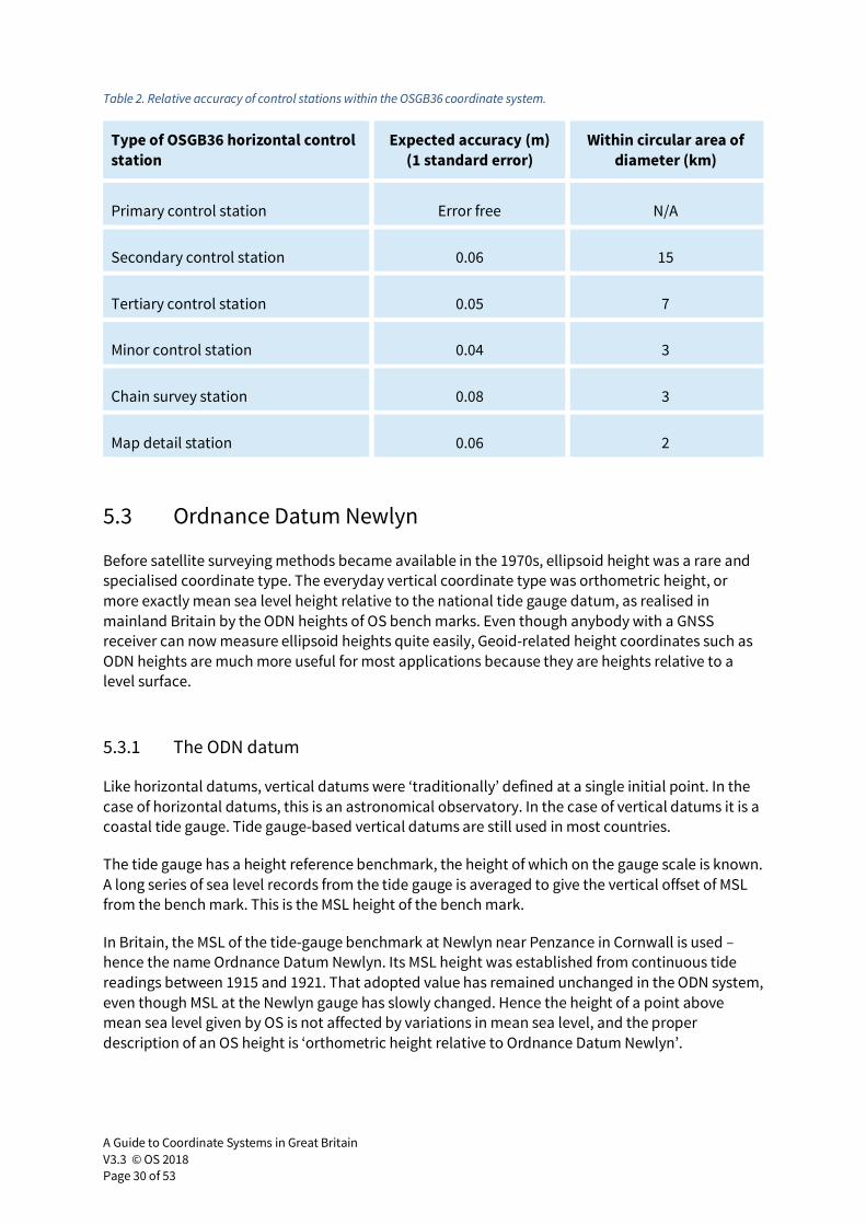
A Guide to Coordinate Systems in Great Britain
V3.3 © OS 2018
Page 30 of 53
Table 2. Relative accuracy of control stations within the OSGB36 coordinate system.
Type of OSGB36 horizontal control
station
Expected accuracy (m)
(1 standard error)
Within circular area of
diameter (km)
Primary control station Error free N/A
Secondary control station 0.06 15
Tertiary control station 0.05 7
Minor control station 0.04 3
Chain survey station 0.08 3
Map detail station 0.06 2
5.3 Ordnance Datum Newlyn
Before satellite surveying methods became available in the 1970s, ellipsoid height was a rare and
specialised coordinate type. The everyday vertical coordinate type was orthometric height, or
more exactly mean sea level height relative to the national tide gauge datum, as realised in
mainland Britain by the ODN heights of OS bench marks. Even though anybody with a GNSS
receiver can now measure ellipsoid heights quite easily, Geoid-related height coordinates such as
ODN heights are much more useful for most applications because they are heights relative to a
level surface.
5.3.1 The ODN datum
Like horizontal datums, vertical datums were ‘traditionally’ defined at a single initial point. In the
case of horizontal datums, this is an astronomical observatory. In the case of vertical datums it is a
coastal tide gauge. Tide gauge-based vertical datums are still used in most countries.
The tide gauge has a height reference benchmark, the height of which on the gauge scale is known.
A long series of sea level records from the tide gauge is averaged to give the vertical offset of MSL
from the bench mark. This is the MSL height of the bench mark.
In Britain, the MSL of the tide-gauge benchmark at Newlyn near Penzance in Cornwall is used –
hence the name Ordnance Datum Newlyn. Its MSL height was established from continuous tide
readings between 1915 and 1921. That adopted value has remained unchanged in the ODN system,
even though MSL at the Newlyn gauge has slowly changed. Hence the height of a point above
mean sea level given by OS is not affected by variations in mean sea level, and the proper
description of an OS height is ‘orthometric height relative to Ordnance Datum Newlyn’.
A Guide to Coordinate Systems in Great Britain
V3.3 © OS 2018
Page 31 of 53
5.3.2 The ODN TRF
A network of about 200 fundamental bench marks for height measurement was constructed across
Britain in the first half of the twentieth century. These are underground chambers containing a
height reference object, topped by a small pillar on which is another reference point. The idea is
that the point on the top is easy to access for normal use, whereas the hidden underground mark is
less susceptible to damage.
The orthometric height of each fundamental bench mark relative to Newlyn was determined by a
network of precise levelling lines across Britain. You can find descriptions of the precise levelling
technique in land surveying textbooks. This technique is capable of transferring orthometric height
from one point to another with an error of less than 2 x √d millimetres, where d is the distance
levelled in kilometres. Today, the accuracy of the precise levelling technique is rivalled by the
combination of GNSS ellipsoid heighting with a precise gravimetric Geoid model that allows the
ellipsoid height difference between two points to be easily converted to an orthometric height
difference.
The ODN TRF was subsequently densified by less precise levelling to obtain the heights of about
three-quarters of a million Ordnance Survey bench marks all over Britain. These lower-order bench
marks are often seen cut into stone at the base of a building, church or bridge. About half a million
of them are in existence and usable today. An important error source to bear in mind is possible
subsidence of Ordnance Survey bench marks, especially in areas where mining has caused
collapse of the ground. In these areas, cases of bench mark subsidence of several metres have
been reported.
5.3.3 Relative accuracy of ODN bench marks
The following table is a statistical statement of ODN bench mark accuracy relative to other bench
marks in the same area. The primary layer of the ODN TRF consists of the fundamental bench
marks, which are considered error-free within the ODN coordinate system. The Ordnance Survey
National Geoid Model (see section 6.4 below) relates ODN orthometric heights to the GNSS
ellipsoid GRS80. Table 3 shows the expected maximum levelling error between bench marks on
the same levelling line. This only describes the original measurement error. The Ordnance Survey
bench mark network has not been maintained since the 1970s, so beware of possible bench mark
subsidence.
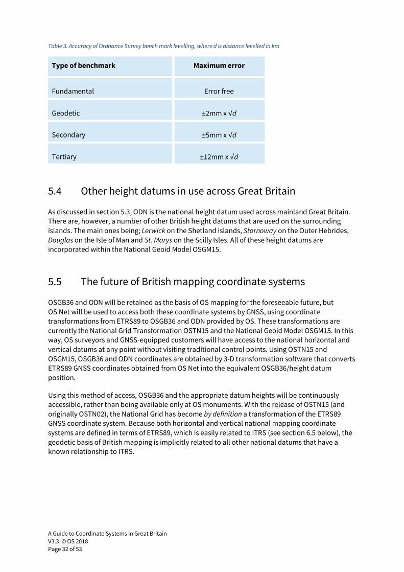
A Guide to Coordinate Systems in Great Britain
V3.3 © OS 2018
Page 32 of 53
Table 3. Accuracy of Ordnance Survey bench mark levelling, where d is distance levelled in km
Type of benchmark Maximum error
Fundamental Error free
Geodetic ±2mm x √d
Secondary ±5mm x √d
Tertiary ±12mm x √d
5.4 Other height datums in use across Great Britain
As discussed in section 5.3, ODN is the national height datum used across mainland Great Britain.
There are, however, a number of other British height datums that are used on the surrounding
islands. The main ones being; Lerwick on the Shetland Islands, Stornoway on the Outer Hebrides,
Douglas on the Isle of Man and St. Marys on the Scilly Isles. All of these height datums are
incorporated within the National Geoid Model OSGM15.
5.5 The future of British mapping coordinate systems
OSGB36 and ODN will be retained as the basis of OS mapping for the foreseeable future, but
OS Net will be used to access both these coordinate systems by GNSS, using coordinate
transformations from ETRS89 to OSGB36 and ODN provided by OS. These transformations are
currently the National Grid Transformation OSTN15 and the National Geoid Model OSGM15. In this
way, OS surveyors and GNSS-equipped customers will have access to the national horizontal and
vertical datums at any point without visiting traditional control points. Using OSTN15 and
OSGM15, OSGB36 and ODN coordinates are obtained by 3-D transformation software that converts
ETRS89 GNSS coordinates obtained from OS Net into the equivalent OSGB36/height datum
position.
Using this method of access, OSGB36 and the appropriate datum heights will be continuously
accessible, rather than being available only at OS monuments. With the release of OSTN15 (and
originally OSTN02), the National Grid has become by definition a transformation of the ETRS89
GNSS coordinate system. Because both horizontal and vertical national mapping coordinate
systems are defined in terms of ETRS89, which is easily related to ITRS (see section 6.5 below), the
geodetic basis of British mapping is implicitly related to all other national datums that have a
known relationship to ITRS.
A Guide to Coordinate Systems in Great Britain
V3.3 © OS 2018
Page 33 of 53
At some point in the future, the drift of the Eurasian tectonic plate (~25mm/year) relative to WGS84
plus the improved accuracy of stand-alone GPS positioning from even simple “consumer level”
receivers will mean the offset between ETRS89 and WGS84 becomes apparent to a much wider
group of users, even on small scale mapping. At this time either a change to the epoch of ETRS89
(to closely align it with WGS84) may have to be considered, or the introduction of a small
transformation to shift WGS84 coordinates back to ETRS89, before then transforming (e.g. with
OSTN15) to OSGB36.
The coordinates and other information of the traditional networks are no longer actively
maintained by OS. Access to these traditional control archives is made available through online
services on the OS website.
6 From one coordinate system to another:
geodetic transformations
6.1 What is a geodetic transformation?
A geodetic transformation is a mathematical operation that takes the coordinates of a point in one
coordinate system and returns the coordinates of the same point in a second coordinate system.
Hopefully we will also have an ‘inverse transformation’ to get back to the first coordinate system
from given coordinates in the second. Many types of mathematical operation are used to
accomplish this task. The term ‘geodetic transformation’ does not indicate a particular type of
formula.
To properly understand geodetic transformations, it is essential to understand the relationship
between a datum and the TRF that realises the datum. Having looked at several examples of real
TRFs in sections 4 and 5, we know that they are of widely variable quality. Unless a TRF is perfect,
the datum it realises is ambiguous. We can think about this in the following way: the given three-
dimensional coordinates of any three ground points in the TRF imply the location of the
coordinate origin, and the orientation of the coordinate axes, relative to those three points. If we
select a different set of three ground points, the origin and orientation implied will be slightly
different. This is due to observational errors in the determination of the coordinates of the ground
points. Taking the TRF as a whole, the datum that it implies has some degree of uncertainty,
because the origin positions implied by different selections of TRF ground points are never in
perfect agreement with each other.
The usual situation in geodesy is that we have two TRFs realising two different datums, with a
large number of points in common between the two TRFs. That is, a particular ground point will be
included in both TRFs, but it will have different coordinates in each. Because the TRFs are not
perfect realisations of their respective datums, it is impossible to say exactly what the
transformation between the two datums is. We can only give a best estimate of the transformation
with a statistical measure of the quality of the estimate.
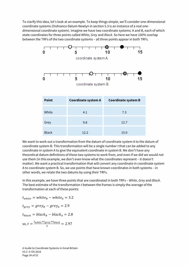
A Guide to Coordinate Systems in Great Britain
V3.3 © OS 2018
Page 34 of 53
To clarify this idea, let’s look at an example. To keep things simple, we’ll consider one-dimensional
coordinate systems (Ordnance Datum Newlyn in section 5.3 is an instance of a real one-
dimensional coordinate system). Imagine we have two coordinate systems: A and B, each of which
state coordinates for three points called White, Grey and Black. So here we have 100% overlap
between the TRFs of the two coordinate systems – all three points appear in both TRFs.
Point Coordinate system A Coordinate system B
White 4.1 7.3
Grey 9.8 12.7
Black 12.2 15.0
We want to work out a transformation from the datum of coordinate system A to the datum of
coordinate system B. This transformation will be a single number t that can be added to any
coordinate in system A to give the equivalent coordinate in system B. We don’t have any
theoretical datum definitions of these two systems to work from, and even if we did we would not
use them (in this example, we don’t even know what the coordinates represent – it doesn’t
matter). We want a practical transformation that will convert any coordinate in coordinate system
A to coordinate system B. So, we use points that have known coordinates in both systems – in
other words, we relate the two datums by using their TRFs.
In this example, we have three points that are coordinated in both TRFs – White, Grey and Black.
The best estimate of the transformation t between the frames is simply the average of the
transformation at each of these points:
������ = �ℎ���� − �ℎ��� = 3.2
����� = ����� − ���� = 2.9
�!"#$% = &'()*� − &'()* = 2.8
so, � = �,-./01�23041�56789: = 2.97
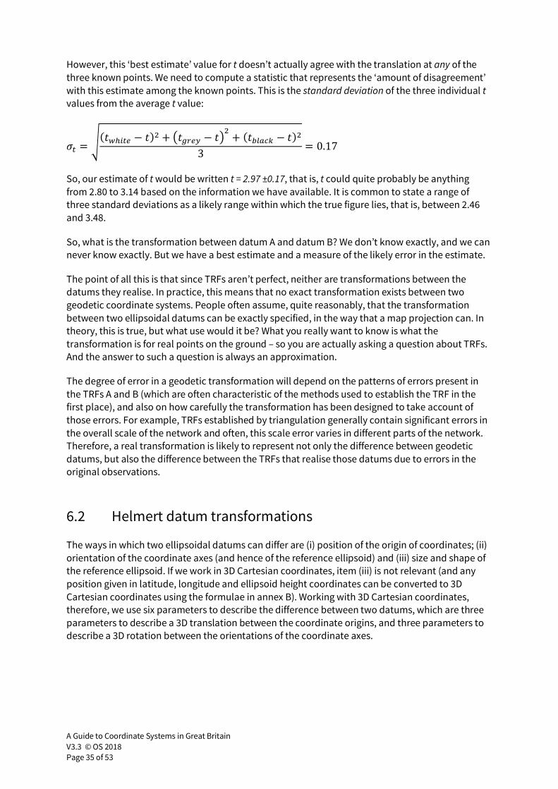
A Guide to Coordinate Systems in Great Britain
V3.3 © OS 2018
Page 35 of 53
However, this ‘best estimate’ value for t doesn’t actually agree with the translation at any of the
three known points. We need to compute a statistic that represents the ‘amount of disagreement’
with this estimate among the known points. This is the standard deviation of the three individual t
values from the average t value:
<� = =������� − ��> + ?����� − �@> + ��!"#$% − ��>3 = 0.17
So, our estimate of t would be written t = 2.97 ±0.17, that is, t could quite probably be anything
from 2.80 to 3.14 based on the information we have available. It is common to state a range of
three standard deviations as a likely range within which the true figure lies, that is, between 2.46
and 3.48.
So, what is the transformation between datum A and datum B? We don’t know exactly, and we can
never know exactly. But we have a best estimate and a measure of the likely error in the estimate.
The point of all this is that since TRFs aren’t perfect, neither are transformations between the
datums they realise. In practice, this means that no exact transformation exists between two
geodetic coordinate systems. People often assume, quite reasonably, that the transformation
between two ellipsoidal datums can be exactly specified, in the way that a map projection can. In
theory, this is true, but what use would it be? What you really want to know is what the
transformation is for real points on the ground – so you are actually asking a question about TRFs.
And the answer to such a question is always an approximation.
The degree of error in a geodetic transformation will depend on the patterns of errors present in
the TRFs A and B (which are often characteristic of the methods used to establish the TRF in the
first place), and also on how carefully the transformation has been designed to take account of
those errors. For example, TRFs established by triangulation generally contain significant errors in
the overall scale of the network and often, this scale error varies in different parts of the network.
Therefore, a real transformation is likely to represent not only the difference between geodetic
datums, but also the difference between the TRFs that realise those datums due to errors in the
original observations.
6.2 Helmert datum transformations
The ways in which two ellipsoidal datums can differ are (i) position of the origin of coordinates; (ii)
orientation of the coordinate axes (and hence of the reference ellipsoid) and (iii) size and shape of
the reference ellipsoid. If we work in 3D Cartesian coordinates, item (iii) is not relevant (and any
position given in latitude, longitude and ellipsoid height coordinates can be converted to 3D
Cartesian coordinates using the formulae in annex B). Working with 3D Cartesian coordinates,
therefore, we use six parameters to describe the difference between two datums, which are three
parameters to describe a 3D translation between the coordinate origins, and three parameters to
describe a 3D rotation between the orientations of the coordinate axes.
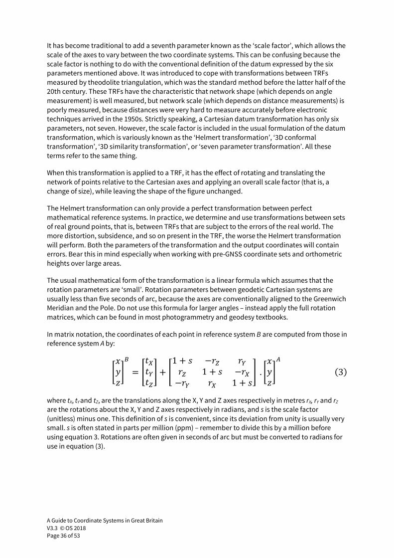
A Guide to Coordinate Systems in Great Britain
V3.3 © OS 2018
Page 36 of 53
It has become traditional to add a seventh parameter known as the ‘scale factor’, which allows the
scale of the axes to vary between the two coordinate systems. This can be confusing because the
scale factor is nothing to do with the conventional definition of the datum expressed by the six
parameters mentioned above. It was introduced to cope with transformations between TRFs
measured by theodolite triangulation, which was the standard method before the latter half of the
20th century. These TRFs have the characteristic that network shape (which depends on angle
measurement) is well measured, but network scale (which depends on distance measurements) is
poorly measured, because distances were very hard to measure accurately before electronic
techniques arrived in the 1950s. Strictly speaking, a Cartesian datum transformation has only six
parameters, not seven. However, the scale factor is included in the usual formulation of the datum
transformation, which is variously known as the ‘Helmert transformation’, ‘3D conformal
transformation’, ‘3D similarity transformation’, or ‘seven parameter transformation’. All these
terms refer to the same thing.
When this transformation is applied to a TRF, it has the effect of rotating and translating the
network of points relative to the Cartesian axes and applying an overall scale factor (that is, a
change of size), while leaving the shape of the figure unchanged.
The Helmert transformation can only provide a perfect transformation between perfect
mathematical reference systems. In practice, we determine and use transformations between sets
of real ground points, that is, between TRFs that are subject to the errors of the real world. The
more distortion, subsidence, and so on present in the TRF, the worse the Helmert transformation
will perform. Both the parameters of the transformation and the output coordinates will contain
errors. Bear this in mind especially when working with pre-GNSS coordinate sets and orthometric
heights over large areas.
The usual mathematical form of the transformation is a linear formula which assumes that the
rotation parameters are ‘small’. Rotation parameters between geodetic Cartesian systems are
usually less than five seconds of arc, because the axes are conventionally aligned to the Greenwich
Meridian and the Pole. Do not use this formula for larger angles – instead apply the full rotation
matrices, which can be found in most photogrammetry and geodesy textbooks.
In matrix notation, the coordinates of each point in reference system B are computed from those in
reference system A by:
BC�DE� = F�G�H�IJ + F1 + K −�I �H�I 1 + K −�G−�H �G 1 + KJ. B
C�DE �3�
where tX, tY and tZ, are the translations along the X, Y and Z axes respectively in metres rX, rY and rZ
are the rotations about the X, Y and Z axes respectively in radians, and s is the scale factor
(unitless) minus one. This definition of s is convenient, since its deviation from unity is usually very
small. s is often stated in parts per million (ppm) – remember to divide this by a million before
using equation 3. Rotations are often given in seconds of arc but must be converted to radians for
use in equation (3).
A Guide to Coordinate Systems in Great Britain
V3.3 © OS 2018
Page 37 of 53
Beware that two opposite conventions are in use regarding the rotation parameters of the Helmert
transformation. The form of transformation as given in equation (3) is referred to as the “Position
Vector transformation”. It is the form in most common use in Europe (particularly in the oil and gas
industry), is used by the International Association of Geodesy (IAG) and recommended by ISO
19111 and is EPSG dataset coordinate operation method code 1033. The form of transformation
that uses opposite rotation signs to those in equation (3) is referred to as the “Coordinate Frame
Rotation transformation” and is common in the USA oil and gas industry and is EPSG dataset
coordinate operation method code 1032. If there is any ambiguity about which convention applies
it is best, for safety, to always include a test point with coordinates in systems A and B when
stating a transformation.
Sometimes, three-parameter (translation only) or six-parameter (translation and rotation only)
transformations are encountered, which omit some of the seven parameters used here. The same
formula can be used to apply these transformations, setting parameters not used to zero.
Any ‘small’ Helmert transformation can be reversed by simply changing the signs of all the
parameters and applying equation (3). This is valid only when the changes in coordinates due to
the transformation are very small compared to the size of the network.
The Helmert transformation is designed to transform between two datums, and it cannot really
cope with distortions in TRFs. As we’ve seen, in practice, we want an accurate transformation
between the coordinates of points on the ground in the two coordinate systems for the area we’re
interested in. If there are large regional distortions present in one or both of the TRFs, a single set
of Helmert parameters for the whole coordinate system will not accomplish this. For the
transformation from ETRS89 to OSGB36 in Britain, using a single Helmert transformation will give
errors of up to 3m (95%) in plan and 3.5m (95%) plan and height, depending where in the country
the points of interest are. One solution to this is to compute a special set of Helmert parameters for
a particular region – this is known as a ‘local transformation’. Alternatively, more complex
transformation types that model TRF distortion can be used. An example of this is the National
Grid Transformation OSTN15 discussed in section 6.3 below.
To summarise: For a simple datum change of latitude and longitude coordinates from datum A to
datum B, first convert to Cartesian coordinates (formulae in annex B), taking all ellipsoid heights as
zero and using the ellipsoid parameters of datum A; then apply a Helmert transformation from
datum A to datum B using equation (3); finally convert back to latitude and longitude using the
ellipsoid parameters of datum B (formulae in annex C) discarding the datum B ellipsoid height.
There is a worked example Helmert transformation in annex D.
NOTE: Molodensky datum transformations: there are formulae to change between geodetic datums when the positions of points are expressed as latitude and longitude coordinates, without first converting the positions to Cartesian coordinates. These are known as the Full Molodensky formulae or the Abridged Molodensky formulae, the latter having a lower degree of accuracy. However, the Molodensky formulae cannot cope with a difference in orientation of the ellipsoid axes – it only deals with a translation of the origin and changes in ellipsoid size and shape. For this reason, the Molodensky formulae are not given here.
A Guide to Coordinate Systems in Great Britain
V3.3 © OS 2018
Page 38 of 53
6.3 National Grid Transformation OSTN15 (ETRS89–OSGB36)
To cope with the distortions in the OSGB36 TRF, different transformations are needed in different
parts of the country. For this reason, the national standard datum transformation between
OSGB36 and ETRS89 is not a simple Helmert datum transformation. Instead, Ordnance Survey has
developed a ‘rubber-sheet’ style transformation that works with a transformation grid expressed
in easting and northing coordinates. The grids of northing and easting shifts between ETRS89 and
OSGB36 cover Britain at a resolution of one kilometre. From these grids, a northing and easting
shift for each point to be transformed is obtained by a bilinear interpolation. This is called the
National Grid Transformation OSTN15, and it is freely available, as an online service, a software
package or as raw data for developers, from the Ordnance Survey website.
The National Grid Transformation copes not only with the change of datum between the two
coordinate systems, but also with the TRF distortions in the OSGB36 triangulation network, which
make a simple datum transformation of the Helmert type limited to applications requiring an
accuracy level of only about 3 metres. OSTN15 removes the need to estimate local Helmert
transformations between ETRS89 and OSGB36 for particular locations.
Because the National Grid Transformation works with easting and northing coordinates, other
ETRS89 coordinate types (3D Cartesian or latitude and longitude) must first be converted to
eastings and northings. This is done using the same map projection as is used for the National Grid
(see section 7 below), except that the GRS80 ellipsoid rather than the Airy 1830 ellipsoid is used.
The parameters and formulae required to obtain these ETRS89 eastings and northings are given in
annexes A to C. After the transformation, the resulting National Grid eastings and northings can be
converted back to latitude and longitude (this time using the Airy ellipsoid) if required.
OSTN15 is the definitive OSGB36/ETRS89 transformation. OSTN15 in combination with the ETRS89
coordinates of the OS Net stations, rather than the old triangulation network, define the National
Grid. This means that, for example, the National Grid coordinates of an existing OSGB36 point,
refixed using GNSS from OS Net and OSTN15, will be the correct ones. The original archived
OSGB36 National Grid coordinates of the point (if different) will be wrong, by definition, but the
two coordinates (new and archived) will agree on average to better than 0.1m (0.1m rmse, 68%
probability).
6.4 National Geoid Model OSGM15 (ETRS89-Orthometric height)
A vertical transformation between ETRS89 ellipsoid height and orthometric height is also available
from Ordnance Survey. This transformation is based on a gravimetric Geoid model covering
Great Britain, Ireland and Northern Ireland aligned with their respective vertical datums. In
mainland Britain, OSGM15 therefore gives Ordnance Datum Newlyn (ODN) orthometric heights
directly from GNSS survey for direct compatibility with OS mapping, without the surveyor having
to visit Ordnance Survey bench marks.
OSGM15 also covers areas of Britain not related to ODN such as the Orkney Islands, Shetland Isles,
Outer Hebrides, Scilly Isles and the Isle of Man. Orthometric heights in these areas are related to
specific local vertical datums.
A Guide to Coordinate Systems in Great Britain
V3.3 © OS 2018
Page 39 of 53
In the previous model (OSGM02) all the datums were extended from land to a distance of 10km
offshore and beyond this limit transformation parameters were set to zero. For OSGM15 datums
are extended to just 2km offshore. All areas beyond this are populated with a version of ODN
named “ODN Offshore” to signify its lower quality from ODN on land. This approach avoids the
arbitrary “cliff” in the transformation data at 10km but signifies the extended nature (and
therefore lower quality) of the datum when used offshore. Away from land “ODN Offshore” values
are more closely aligned to the gravimetric geoid rather than the one fitted to the FBMs on land.
The National Geoid Model OSGM15 is a grid of geoid-ellipsoid separation values on the same
1 kilometre resolution grid as the OSTN15 transformation. In the same way as for OSTN15 a geoid-
ellipsoid separation value is obtained for any location by bi-linear interpolation. The nominal
accuracy of the geoid model is 8mm rms (root mean square) in mainland UK, better than 2cm rms
for other areas and 3cm rms for Isle of Man. This transformation is freely available from the OS
website. OS recommends the use of the National Geoid Model OSGM15 and OS Net for high-
accuracy orthometric heighting, in preference to Ordnance Survey bench marks.
6.5 ETRS89 to and from ITRS
The transformations between ETRS89 (European TRS 1989, the Europe-fixed version of WGS84)
and the various versions of the ITRS (International Terrestrial Reference System) are published by
IERS (International Earth Rotation Service) via their Internet site. The easiest way to carry out these
transformations is using the ETRS89/ITRS transformation tool on the EUREF Permanent Network
(EPN) website – http://www.epncb.oma.be/_productsservices/coord_trans/.
The usual application of these transformations is in dealing with GNSS coordinates determined in
a ‘fiducial network’ using IGS permanent stations as fixed control points and using IGS products
such as satellite ephemerides, satellite clock solutions and Earth orientation parameters. In this
application, the coordinates adopted for the fixed IGS stations should be ITRS coordinates in the
same realisation of ITRS as used to determine the IGS precise ephemerides and other products.
The ITRF coordinates of the IGS reference stations at the epoch of observation are obtained by
multiplying the ITRF station velocity by the time difference between the ITRF reference epoch and
epoch of observation and adding this position update to the ITRF reference epoch station
positions.
The resulting coordinates of the unknown stations are in ITRS at the epoch of observation. The
EPN transformation tool referenced above can then be used to obtain coordinates in a frame of
the ETRS89.
6.6 Approximate WGS84 to OSGB36/ODN transformation
The following Helmert parameters transform WGS84 (or ETRS89 or ITRS, the differences are
negligible here) coordinates to ‘something like’ OSGB36 and ‘something like’ ODN heights. The
error is up to 3.5 metres (95%) both horizontally and vertically. This transformation is for use with
equation (3). Note the remarks made about Helmert transformations in section 6.2.
A Guide to Coordinate Systems in Great Britain
V3.3 © OS 2018
Page 40 of 53
Table 4. ETRS89 (WGS84) to OSGB36/ODN Helmert transformation parameters.
tX(m) tY(m) tZ(m) s (ppm) rX(sec) rY(sec) rZ(sec)
- 446.448 + 125.157 - 542.060 + 20.4894 - 0.1502 - 0.2470 - 0.8421
NOTE 1: OSGB36 is an inhomogeneous TRF by modern standards. Do not use this transformation
for applications requiring better than 3.5 metre (95%) accuracy in the transformation step,
either vertically or horizontally. Do not use it for points outside Britain.
NOTE 2: OSGB36 does not exist offshore.
6.7 Transformation between OS Net v2001 and v2009
realisations
As detailed in section 5.1 the OS Net ETRS89 realisation was originally related to ITRF97 at epoch
2001.553. This original realisation is now designated “OS Net v2001”. In 2016 it was updated to a
realisation related to ITRF97 at epoch 2009.756, designated “OS Net v2009”. The average shift
between the two sets of coordinates is small (rms of all components ~18mm). A file of the shifts for
individual OS Net stations is available on the OS website. The transformation parameters below
can also be used (with equation 3 from section 6.2) to move any coordinates related to OS Net
v2001 to be compatible with OS Net v2009.
Table 5. OS Net v2001 to OS Net v2009 Helmert transformation parameters.
tX(m) tY(m) tZ(m) s (ppm) rX(sec) rY(sec) rZ(sec)
+ 0.0054 - 0.0117 - 0.0010 + 0.000 + 0.0000 + 0.0000 + 0.0000
NOTE The overall RMS of this transformation, when computed from the two OS Net data sets, is
12.2mm. The RMS residual components in the East, North, Up system are 6.9mm, 9.2mm,
17.8mm respectively.
There is a range of options for transforming coordinates computed under OS Net v2001 to be more
compatible with OS Net v2009. In increasing order of accuracy they are:
1 Apply the 3 parameter transformation given in Table 5 above.
2 Apply a simple mean shift in X, Y and Z based on the nearest n OS Net stations with n based on
the most likely number of OS Net stations used in the original processing. The OS Net station
coordinate shifts (in X, Y, Z) are in a file on the OS web site. Both v2001 and v2009 coordinates
are given in the OS Net coordinate file on the OS web site so shifts can also be computed from
there.
3 (Equal accuracy to 4 below). Apply weighted mean shifts based on the nearest n OS Net stations
with n based on the most likely number of OS Net stations used in the original processing.
Weighting can be based on the distance to the OS Net stations.
4 (Equal accuracy to 3 above). Apply a simple mean shift in X, Y and Z based on the OS Net
stations actually used in the processing.
A Guide to Coordinate Systems in Great Britain
V3.3 © OS 2018
Page 41 of 53
5 Apply weighted mean shifts based on the OS Nets actually used in the processing. Weighting
can be based on the distance to the OS Net stations.
6 Re-process the raw GNSS data using the OS Net v2009 coordinates.
7 Transverse Mercator map projections
When features on the curved surface of the Earth are represented on a plane surface, distortions of
distances, angles or both are inevitable. Originally the ‘plane surface’ was a map sheet; now it is
often the plane coordinate system of GIS software. A map projection is any function that converts
ellipsoidal latitude and longitude coordinates to plane easting and northing coordinates. OS maps
use a type of projection known as the Transverse Mercator (TM). The same type of projection is
used in a worldwide mapping standard known as Universal Transverse Mercator (UTM). The
parameters of the National Grid TM and UTM projections are given in annexe A.
The TM projection can be thought of as a sheet of paper carrying the mapping grid (of eastings and
northings), which is curved so as to touch the ellipsoid along a certain line. This line of contact is
chosen to be a north-south central meridian. Points on the ellipsoid are projected onto the curved
sheet, giving easting and northing coordinates for each point. The effect is to distort the distance
between projected points, except on the central meridian, where the ellipsoid touches the
mapping grid. This scale distortion effect increases east and west of the central meridian. The
scale distortion can be measured by a local scale factor which is 1 on the central meridian and
greater than one everywhere else.
To reduce the worst scale distortion effect in the extreme eastern and western regions of the
mapping area, a scale reduction factor is introduced over the whole mapping area. Strictly this
turns the projection into a “Modified TM”. This makes projected distances on the central meridian
slightly too small, but lessens the scale distortion for points far to the east or west of the central
meridian. With the overall scale reduction applied, there are now two lines (either side of the
central meridian) on which the local scale factor is one. Inside these lines, the local scale factor is
less than one (with a minimum on the central meridian), and outside these lines it is more than
one. On the central meridian, the local scale factor is now equal to the scale reduction factor that
was introduced.
The TM projection used for all OS maps has a central meridian at longitude 2° West and a central
meridian scale factor of approximately 0.9996 (see annexe A for exact value). The two lines of true
scale are about 180 km to the east and west of the central meridian. The stated scale of an OS map
is only exactly true on these lines of true scale, but the scale error elsewhere is quite small. For
instance, the true scale of OS 1:50 000 scale map sheets is actually between 1:49 980 and 1:50 025
depending on easting.
The UTM projections are a way of mapping the whole world in a systematic way by dividing the
Earth by longitude into 60 zones, each 6 degrees of longitude wide. The 60 UTM zones each have a
different central meridian. The zones relevant to British mapping are 29 (central meridian 9° W), 30
(central meridian 3° W) and 31 (central meridian 3° E). The scale on the central meridian is 0.9996
for all UTM zones. The International 1924 ellipsoid was commonly used in the UTM projection in
Europe, but other ellipsoids can also be used with the WGS84 ellipsoid being increasing popular.
When working with UTM coordinates always check which ellipsoid is being used.

A Guide to Coordinate Systems in Great Britain
V3.3 © OS 2018
Page 42 of 53
Annexe C gives formulae for conversion between latitude and longitude and TM eastings and
northings. Annexe A gives the TM parameters for the National Grid and the British UTM zones.
7.1 The National Grid reference convention
The map projection used on OS Great Britain maps is known as the National Grid. The TM eastings
and northings axes are given a ‘false origin’ just south west of the Scilly Isles to ensure that all
coordinates in Britain are positive. The false origin is 400 km west and 100 km north of the ‘true
origin’ on the central meridian at 49°N 2°W.
To reduce the number of figures needed to give a National Grid reference, the grid is divided into
100 km squares, which each have a two-letter code. National Grid positions can be given with this
code followed by an easting between 0 and 100 000 m and a northing between 0 and 100 000 m.
Figure 8. The National Grid, showing the true origin (t.o.) and false origin (f.o.).
A Guide to Coordinate Systems in Great Britain
V3.3 © OS 2018
Page 43 of 53
8 Further information
Quite a lot of information on this subject is available on the Internet. You might find online
implementations of the formulae given in the annexes, although beware that OS does not check or
endorse these. Here are a few addresses directly related to the information in this booklet:
• https://www.ordnancesurvey.co.uk/business-and-government/products/os-net/index.html this
is the OS Net website and contains information and access to data for users of GNSS in GB.
• http://earth-info.nga.mil/GandG/coordsys/csat_pubs.html is the US NGA Geodesy and
Geophysics department publications page. This has lots of information on the WGS84 datum
and the EGM96 global Geoid model.
• http://www.igs.org/ is the IGS home page. This gives access to all the IGS products and
information about them.
• http://www.euref.eu/ is the EUREF home page. EUREF is the governing body of the ETRS89
coordinate system.
• http://www.epncb.oma.be/ is the home page of the EPN (EUREF Permanent Network). It gives
access details for all EPN data and products as well as information on European reference
frames and transformations.
• https://www.iers.org/IERS/EN/Home/home_node.html is the home page of the IERS
(International Earth Rotation and Reference Systems Service) and gives access to information
about the ITRS and ITRF realisations.
• http://www.ordnancesurvey.co.uk/oswebsite/gi/nationalgrid/nghelp1.html is an interactive
guide to the National Grid on the OS website.
• https://www.ordnancesurvey.co.uk/docs/ebooks/history-retriangulation-great-britain-1935-
1962.pdf is a copy of “The History of the Retriangulation of Great Britain 1935 - 1962”. NOTE –
this is a large file (>150Mb).
Here are a few book titles on geodesy, GNSS surveying, and map projections:
• Introduction to geodesy: The history and concepts of modern geodesy by James R Smith,
published by John Wiley & Sons, 1997.
• Geodesy: The concepts by Petr Vanicek and Edward Krakiwsky, published by North Holland
1982.
• GPS satellite surveying 4th edition by Alfred Leick, Lev Rapoport, Dmitry Tatarnikov published
by John Wiley and Sons 2015
• GPS Theory and Practice, 5th revised edition, by B Hofmann-Wellenhof, H Lichtenegger and J
Collins, published by Springer-Verlag 2001.
• Map Projections: Theory and Applications by Frederick Pearson, published by CRC Press 1990.
• Map Projections: A Reference Manual by Lev Bugayevskiy and John Snyder, published by Taylor
and Francis 1995.
Specific enquiries concerning the OS coordinate systems, OS Net, the National Grid transformation
and the National Geoid Model can be directed to the OS Customer Service Centre via the “Contact
us” form on the OS web site at https://www.ordnancesurvey.co.uk/contact/index.html or
telephone +44 (0) 3456 05 05 05.
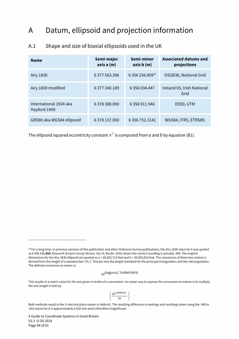
A Guide to Coordinate Systems in Great Britain
V3.3 © OS 2018
Page 44 of 53
A Datum, ellipsoid and projection information
A.1 Shape and size of biaxial ellipsoids used in the UK
Name Semi-major
axis a (m)
Semi-minor
axis b (m)
Associated datums and
projections
Airy 1830 6 377 563.396 6 356 256.90910 OSGB36, National Grid
Airy 1830 modified 6 377 340.189 6 356 034.447 Ireland 65, Irish National
Grid
International 1924 aka
Hayford 1909
6 378 388.000 6 356 911.946 ED50, UTM
GRS80 aka WGS84 ellipsoid 6 378 137.000 6 356 752.3141 WGS84, ITRS, ETRS89.
The ellipsoid squared eccentricity constant is computed from a and b by equation (B1).
10 For a long time, in previous versions of this publication and other Ordnance Survey publications, the Airy 1830 value for b was quoted
as 6 356 256.910. Research (Empire Survey Review, Vol. XI, No.84, 1952) shows the correct rounding is actually .909. The original
dimensions for the Airy 1830 ellipsoid are quoted as a = 20,923,713 feet and b = 20,853,810 feet. The conversion of these two metres is
derived from the length of a standard bar (‘O1’). This bar was the length standard for the principal triangulation and the retriangulation.
The defined conversion to metric is:
)48401603.9)((log10 +axis
This results in a metric value for the axis given in tenths of a nanometre. An easier way to express the conversion to metres is to multiply
the axis length in feet by:
10
10 48401603.0
Both methods result in the 3–decimal place values in table A1. The resulting difference in eastings and northings when using the .909 or
.910 values for b is approximately 0.016 mm and is therefore insignificant.
2e
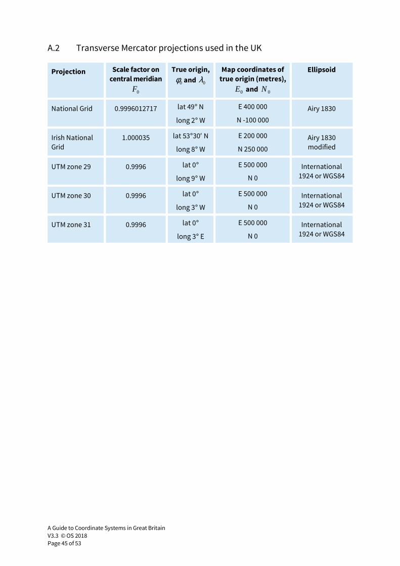
A Guide to Coordinate Systems in Great Britain
V3.3 © OS 2018
Page 45 of 53
A.2 Transverse Mercator projections used in the UK
Projection Scale factor on
central meridian
0F
True origin,
0φ and 0λ
Map coordinates of
true origin (metres),
0E and 0N
Ellipsoid
National Grid 0.9996012717 lat 49° N
long 2° W
E 400 000
N -100 000
Airy 1830
Irish National
Grid
1.000035 lat 53°30′ N
long 8° W
E 200 000
N 250 000
Airy 1830
modified
UTM zone 29 0.9996 lat 0°
long 9° W
E 500 000
N 0
International
1924 or WGS84
UTM zone 30 0.9996 lat 0°
long 3° W
E 500 000
N 0
International
1924 or WGS84
UTM zone 31 0.9996 lat 0°
long 3° E
E 500 000
N 0
International
1924 or WGS84
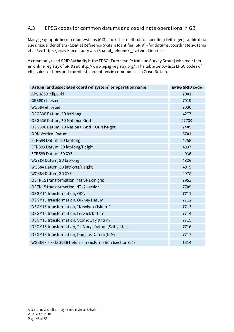
A Guide to Coordinate Systems in Great Britain
V3.3 © OS 2018
Page 46 of 53
A.3 EPSG codes for common datums and coordinate operations in GB
Many geographic information systems (GIS) and other methods of handling digital geographic data
use unique identifiers - Spatial Reference System Identifier (SRID) - for datums, coordinate systems
etc.. See https://en.wikipedia.org/wiki/Spatial_reference_system#Identifier
A commonly used SRID Authority is the EPSG (European Petroleum Survey Group) who maintain
an online registry of SRIDs at http://www.epsg-registry.org/ . The table below lists EPSG codes of
ellipsoids, datums and coordinate operations in common use in Great Britain.
Datum (and associated coord ref system) or operation name EPSG SRID code
Airy 1830 ellipsoid 7001
GRS80 ellipsoid 7019
WGS84 ellipsoid 7030
OSGB36 Datum, 2D lat/long 4277
OSGB36 Datum, 2D National Grid 27700
OSGB36 Datum, 3D National Grid + ODN height 7405
ODN Vertical Datum 5701
ETRS89 Datum, 2D lat/long 4258
ETRS89 Datum, 3D lat/long/Height 4937
ETRS89 Datum, 3D XYZ 4936
WGS84 Datum, 2D lat/long 4326
WGS84 Datum, 3D lat/long/Height 4979
WGS84 Datum, 3D XYZ 4978
OSTN15 transformation, native 1km grid 7953
OSTN15 transformation, NTv2 version 7709
OSGM15 transformation, ODN 7711
OSGM15 transformation, Orkney Datum 7712
OSGM15 transformation, “Newlyn offshore” 7713
OSGM15 transformation, Lerwick Datum 7714
OSGM15 transformation, Stornoway Datum 7715
OSGM15 transformation, St. Marys Datum (Scilly Isles) 7716
OSGM15 transformation, Douglas Datum (IoM) 7717
WGS84 < - > OSGB36 Helmert transformation (section 6.6) 1314
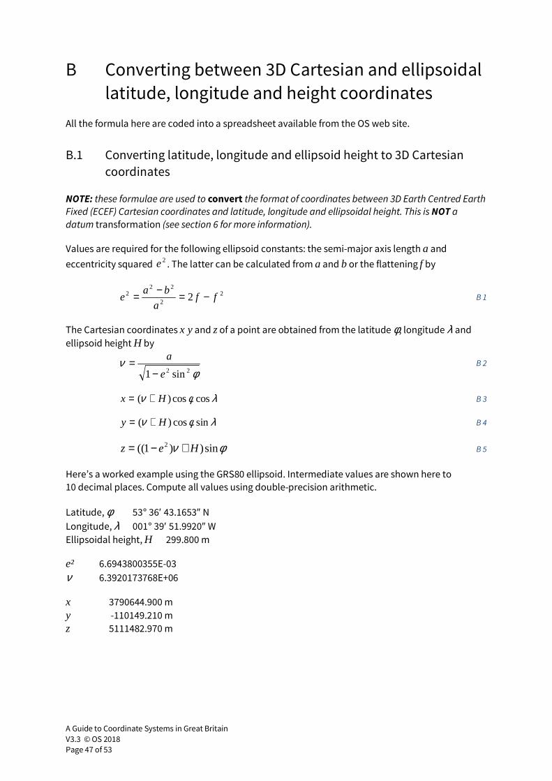
A Guide to Coordinate Systems in Great Britain
V3.3 © OS 2018
Page 47 of 53
B Converting between 3D Cartesian and ellipsoidal
latitude, longitude and height coordinates
All the formula here are coded into a spreadsheet available from the OS web site.
B.1 Converting latitude, longitude and ellipsoid height to 3D Cartesian
coordinates
NOTE: these formulae are used to convert the format of coordinates between 3D Earth Centred Earth Fixed (ECEF) Cartesian coordinates and latitude, longitude and ellipsoidal height. This is NOT a datum transformation (see section 6 for more information).
Values are required for the following ellipsoid constants: the semi-major axis length a and
eccentricity squared . The latter can be calculated from a and b or the flattening f by
B 1
The Cartesian coordinates x y and z of a point are obtained from the latitude φ, longitude λ and
ellipsoid height H by
B 2
B 3
B 4
B 5
Here’s a worked example using the GRS80 ellipsoid. Intermediate values are shown here to
10 decimal places. Compute all values using double-precision arithmetic.
Latitude, φ 53° 36′ 43.1653″ N
Longitude, λ 001° 39′ 51.9920″ W
Ellipsoidal height, H 299.800 m
e² 6.6943800355E-03
ν 6.3920173768E+06
x 3790644.900 m
y -110149.210 m
z 5111482.970 m
2e
22
222 2 ff
a
bae −=−=
φν
22 sin1 e
a
−=
λφν coscos)( Hx +=
λφν sincos)( Hy +=
φν sin))1(( 2 Hez +−=
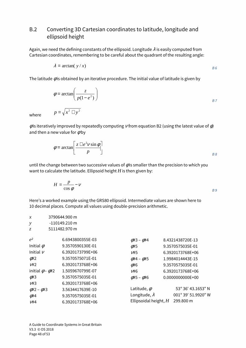
A Guide to Coordinate Systems in Great Britain
V3.3 © OS 2018
Page 48 of 53
B.2 Converting 3D Cartesian coordinates to latitude, longitude and
ellipsoid height
Again, we need the defining constants of the ellipsoid. Longitude λ is easily computed from
Cartesian coordinates, remembering to be careful about the quadrant of the resulting angle:
B 6
The latitude φ is obtained by an iterative procedure. The initial value of latitude is given by
B 7
where
φ is iteratively improved by repeatedly computing ν from equation B2 (using the latest value of φ)
and then a new value for φ by
B 8
until the change between two successive values of φ is smaller than the precision to which you
want to calculate the latitude. Ellipsoid height H is then given by:
B 9
Here’s a worked example using the GRS80 ellipsoid. Intermediate values are shown here to
10 decimal places. Compute all values using double-precision arithmetic.
x 3790644.900 m
y -110149.210 m
z 5111482.970 m
e² 6.6943800355E-03
Initial φ 9.3570590130E-01
Initial ν 6.3920173799E+06
φ#2 9.3570575071E-01
ν#2 6.3920173768E+06
initial φ – φ#2 1.5059670799E-07
φ#3 9.3570575035E-01
ν#3 6.3920173768E+06
φ#2 – φ#3 3.5634417639E-10
φ#4 9.3570575035E-01
ν#4 6.3920173768E+06
φ#3 – φ#4 8.4321438720E-13
φ#5 9.3570575035E-01
ν#5 6.3920173768E+06
φ#4 – φ#5 1.9984014443E-15
φ#6 9.3570575035E-01
ν#6 6.3920173768E+06
φ#5 – φ#6 0.0000000000E+00
Latitude, φ 53° 36′ 43.1653″ N
Longitude, λ 001° 39′ 51.9920″ W
Ellipsoidal height, H 299.800 m
)/arctan( xy=λ
−=
)1(arctan
2ep
zφ
22 yxp +=
+=p
ez φνφ sinarctan
2
νφ
−=cos
pH
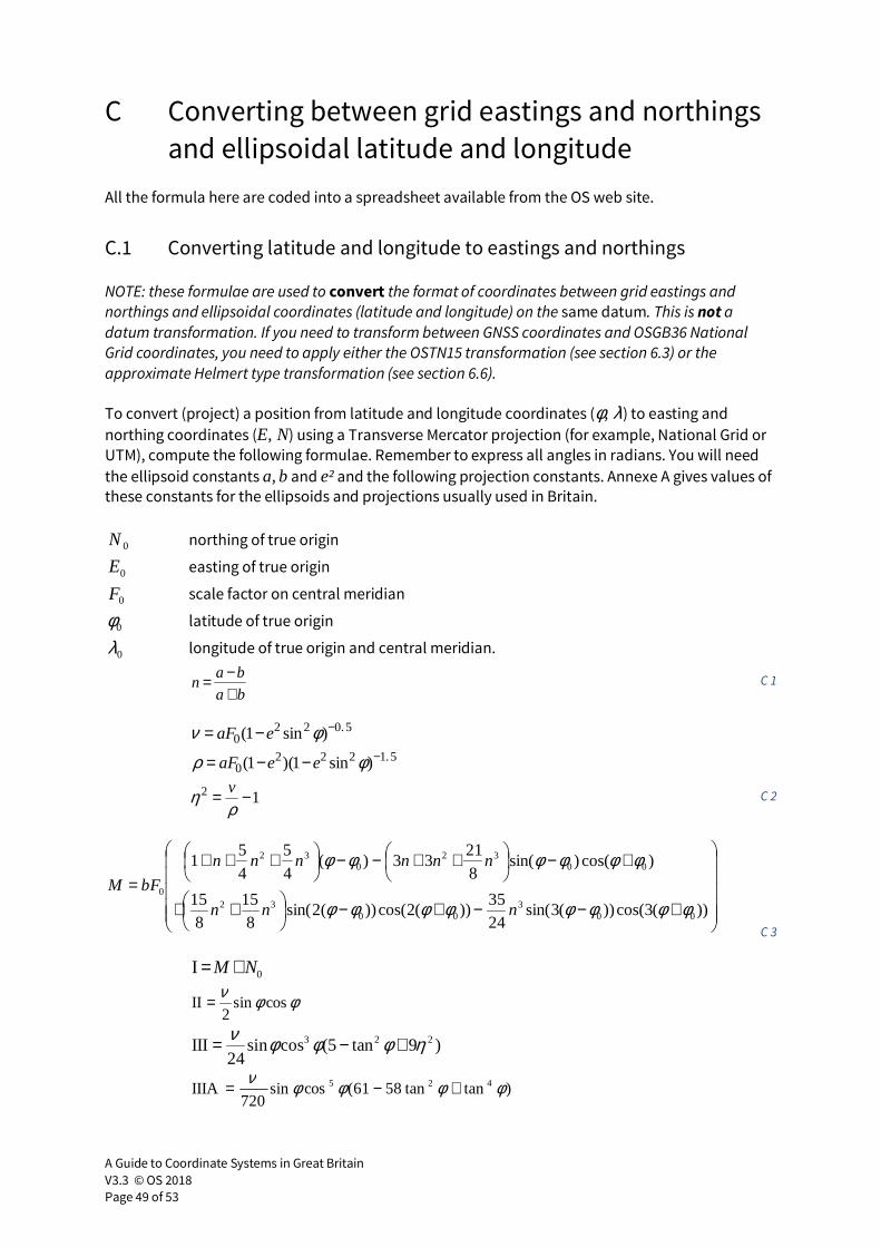
A Guide to Coordinate Systems in Great Britain
V3.3 © OS 2018
Page 49 of 53
C Converting between grid eastings and northings
and ellipsoidal latitude and longitude
All the formula here are coded into a spreadsheet available from the OS web site.
C.1 Converting latitude and longitude to eastings and northings
NOTE: these formulae are used to convert the format of coordinates between grid eastings and northings and ellipsoidal coordinates (latitude and longitude) on the same datum. This is not a datum transformation. If you need to transform between GNSS coordinates and OSGB36 National Grid coordinates, you need to apply either the OSTN15 transformation (see section 6.3) or the approximate Helmert type transformation (see section 6.6).
To convert (project) a position from latitude and longitude coordinates (φ, λ) to easting and
northing coordinates (E, N) using a Transverse Mercator projection (for example, National Grid or
UTM), compute the following formulae. Remember to express all angles in radians. You will need
the ellipsoid constants a, b and e² and the following projection constants. Annexe A gives values of
these constants for the ellipsoids and projections usually used in Britain.
northing of true origin
easting of true origin
scale factor on central meridian
latitude of true origin
longitude of true origin and central meridian.
C 1
C 2
C 3
0N
0E
0F
0φ
0λ
ba
ban
+−=
5.0220 )sin1( −−= φν eaF
5.12220 )sin1)(1( −−−= φρ eeaF
12 −=ρ
η v
+−−+−
++
+−
++−−
+++=
))(3cos())(3sin(2435
))(2cos())(2sin(8
158
15
)cos()sin(8
2133)(
4
5
4
51
003
0032
0032
032
0
φφφφφφφφ
φφφφφφ
nnn
nnnnnn
FbM
0I NM +=
φφνcossin
2II =
)9tan5(cossin24
III 223 ηφφφν +−=
)tantan5861(cossin720
IIIA 425 φφφφν +−=
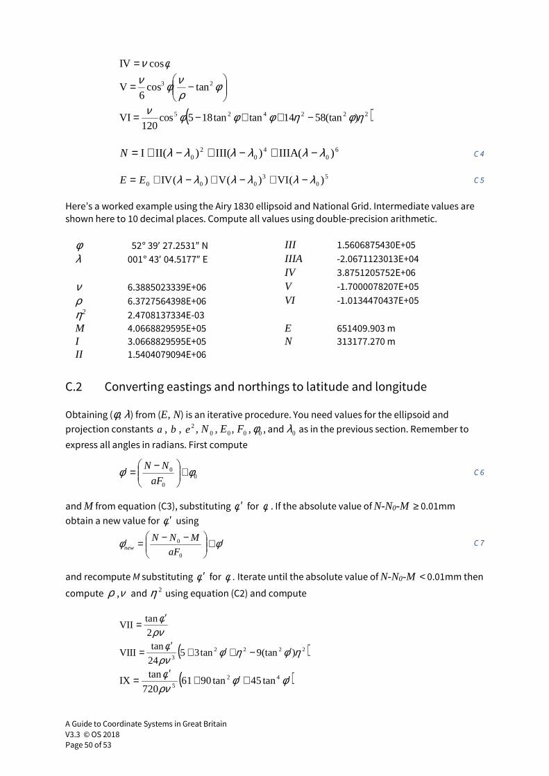
A Guide to Coordinate Systems in Great Britain
V3.3 © OS 2018
Page 50 of 53
C 4
C 5
Here’s a worked example using the Airy 1830 ellipsoid and National Grid. Intermediate values are
shown here to 10 decimal places. Compute all values using double-precision arithmetic.
φ 52° 39′ 27.2531″ N III 1.5606875430E+05
λ 001° 43′ 04.5177″ E IIIA -2.0671123013E+04
IV 3.8751205752E+06
ν 6.3885023339E+06 V -1.7000078207E+05
ρ 6.3727564398E+06 VI -1.0134470437E+05
η2 2.4708137334E-03
M 4.0668829595E+05 E 651409.903 m I 3.0668829595E+05 N 313177.270 m II 1.5404079094E+06
C.2 Converting eastings and northings to latitude and longitude
Obtaining (φ, λ) from (E, N) is an iterative procedure. You need values for the ellipsoid and
projection constants , , , , , , , and as in the previous section. Remember to
express all angles in radians. First compute
C 6
and M from equation (C3), substituting for . If the absolute value of N-N0-M ≥ 0.01mm
obtain a new value for using
C 7
and recompute M substituting for . Iterate until the absolute value of N-N0-M < 0.01mm then
compute , and using equation (C2) and compute
φν cosIV =
−= φ
ρνφν 23 tancos
6V
( )222425 )(tan5814tantan185cos120
VI ηφηφφφν −++−=
60
40
20 )(IIIA)III()(III λλλλλλ −+−+−+=N
50
3000 )(VI)(V)(IV λλλλλλ −+−+−+= EE
a b 2e 0N 0E 0F 0φ 0λ
00
0 φφ +
−=′aF
NN
φ ′ φφ ′
φφ ′+
−−=′0
0
aF
MNNnew
φ ′ φρ ν 2η
ρνφ
2
tanVII
′=
( )22223
)(tan9tan3524
tanVIII ηφηφ
ρνφ ′−+′+
′=
( )φφρνφ ′+′+
′= 42
5tan45tan9061
720
tanIX
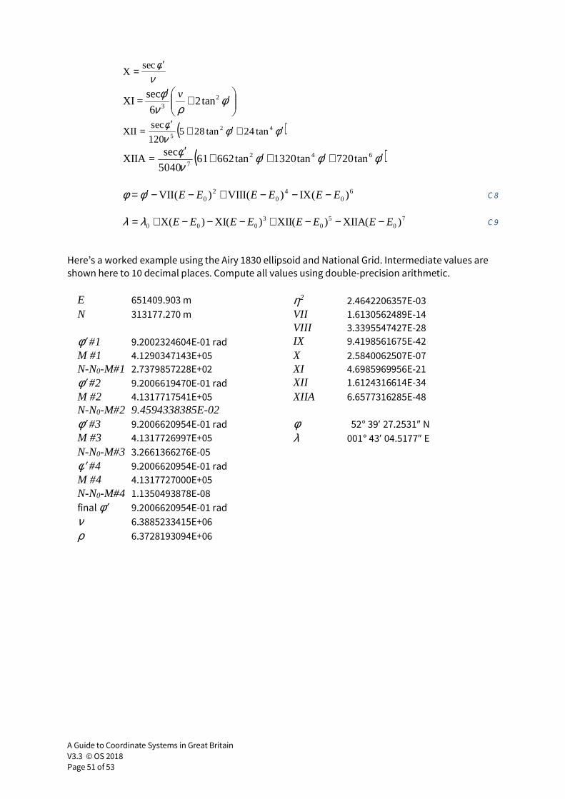
A Guide to Coordinate Systems in Great Britain
V3.3 © OS 2018
Page 51 of 53
C 8
C 9
Here’s a worked example using the Airy 1830 ellipsoid and National Grid. Intermediate values are
shown here to 10 decimal places. Compute all values using double-precision arithmetic.
E 651409.903 m η2 2.4642206357E-03
N 313177.270 m VII 1.6130562489E-14
VIII 3.3395547427E-28
φ′ #1 9.2002324604E-01 rad IX 9.4198561675E-42
M #1 4.1290347143E+05 X 2.5840062507E-07
N-N0-M#1 2.7379857228E+02 XI 4.6985969956E-21
φ′ #2 9.2006619470E-01 rad XII 1.6124316614E-34
M #2 4.1317717541E+05 XIIA 6.6577316285E-48
N-N0-M#2 9.4594338385E-02
φ′ #3 9.2006620954E-01 rad φ 52° 39′ 27.2531″ N
M #3 4.1317726997E+05 λ 001° 43′ 04.5177″ E
N-N0-M#3 3.2661366276E-05
φ′ #4 9.2006620954E-01 rad
M #4 4.1317727000E+05
N-N0-M#4 1.1350493878E-08
final φ′ 9.2006620954E-01 rad
ν 6.3885233415E+06
ρ 6.3728193094E+06
νφ ′
= secX
′+′
φρν
φ 23
tan26
sec=XI
v
( )φφνφ ′+′+
′ 425
tan24tan285120
sec=XII
( )φφφνφ ′+′+′+
′ 6427
tan720tan1320tan662615040
sec=XIIA
60
40
20 )(IX)(VIII)(VII EEEEEE −−−+−−′= φφ
70
50
3000 )(XIIA)(XII)(XI)(X EEEEEEEE −−−+−−−+= λλ
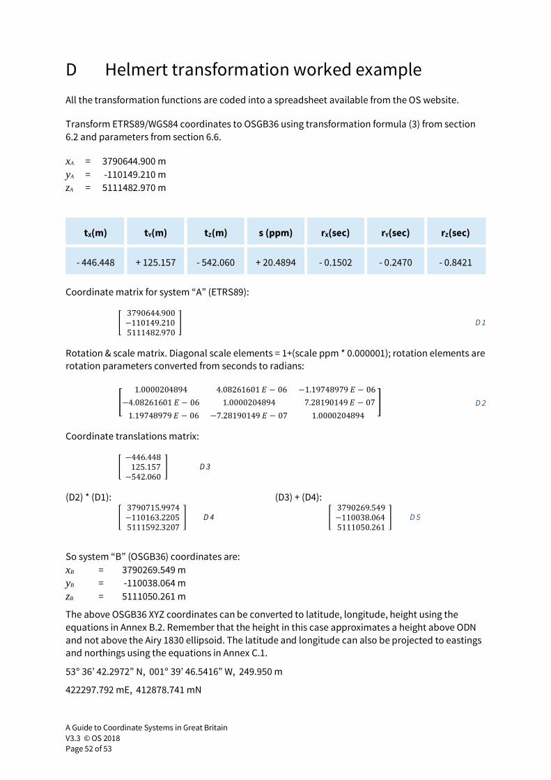
A Guide to Coordinate Systems in Great Britain
V3.3 © OS 2018
Page 52 of 53
D Helmert transformation worked example
All the transformation functions are coded into a spreadsheet available from the OS website.
Transform ETRS89/WGS84 coordinates to OSGB36 using transformation formula (3) from section
6.2 and parameters from section 6.6.
xA = 3790644.900 m
yA = -110149.210 m
zA = 5111482.970 m
tX(m) tY(m) tZ(m) s (ppm) rX(sec) rY(sec) rZ(sec)
- 446.448 + 125.157 - 542.060 + 20.4894 - 0.1502 - 0.2470 - 0.8421
Coordinate matrix for system “A” (ETRS89):
F3790644.900−110149.2105111482.970 J D 1
Rotation & scale matrix. Diagonal scale elements = 1+(scale ppm * 0.000001); rotation elements are
rotation parameters converted from seconds to radians:
B 1.0000204894 4.08261601O − 06 −1.19748979O − 06−4.08261601O − 06 1.0000204894 7.28190149O − 071.19748979O − 06 −7.28190149O − 07 1.0000204894 E D 2
Coordinate translations matrix:
F−446.448125.157−542.060 J D 3
(D2) * (D1): (D3) + (D4):
F3790715.9974−110163.22055111592.3207 J D 4 F3790269.549−110038.0645111050.261 J D 5
So system “B” (OSGB36) coordinates are:
xB = 3790269.549 m
yB = -110038.064 m
zB = 5111050.261 m
The above OSGB36 XYZ coordinates can be converted to latitude, longitude, height using the
equations in Annex B.2. Remember that the height in this case approximates a height above ODN
and not above the Airy 1830 ellipsoid. The latitude and longitude can also be projected to eastings
and northings using the equations in Annex C.1.
53° 36’ 42.2972” N, 001° 39’ 46.5416” W, 249.950 m
422297.792 mE, 412878.741 mN
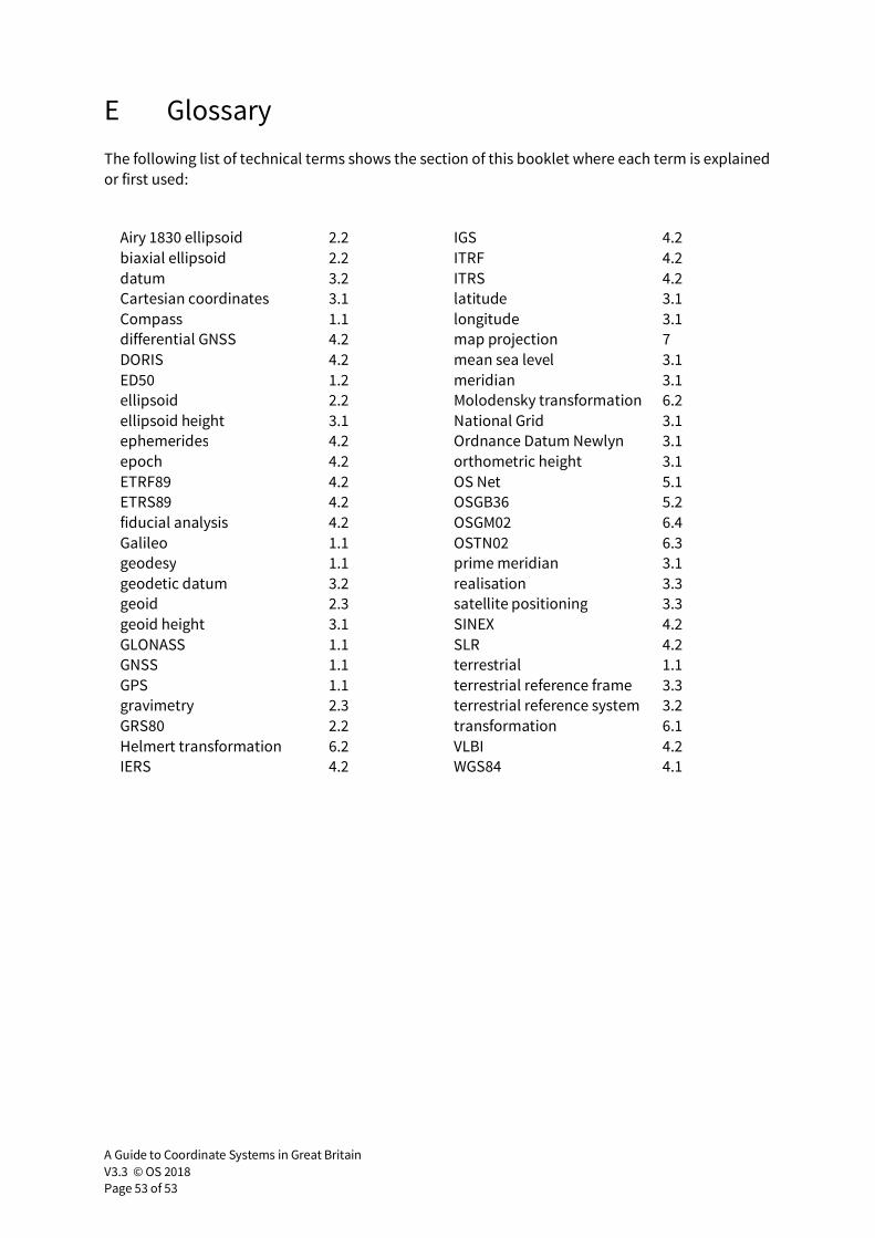
A Guide to Coordinate Systems in Great Britain
V3.3 © OS 2018
Page 53 of 53
E Glossary
The following list of technical terms shows the section of this booklet where each term is explained
or first used:
Airy 1830 ellipsoid 2.2 IGS 4.2
biaxial ellipsoid 2.2 ITRF 4.2
datum 3.2 ITRS 4.2
Cartesian coordinates 3.1 latitude 3.1
Compass 1.1 longitude 3.1
differential GNSS 4.2 map projection 7
DORIS 4.2 mean sea level 3.1
ED50 1.2 meridian 3.1
ellipsoid 2.2 Molodensky transformation 6.2
ellipsoid height 3.1 National Grid 3.1
ephemerides 4.2 Ordnance Datum Newlyn 3.1
epoch 4.2 orthometric height 3.1
ETRF89 4.2 OS Net 5.1
ETRS89 4.2 OSGB36 5.2
fiducial analysis 4.2 OSGM02 6.4
Galileo 1.1 OSTN02 6.3
geodesy 1.1 prime meridian 3.1
geodetic datum 3.2 realisation 3.3
geoid 2.3 satellite positioning 3.3
geoid height 3.1 SINEX 4.2
GLONASS 1.1 SLR 4.2
GNSS 1.1 terrestrial 1.1
GPS 1.1 terrestrial reference frame 3.3
gravimetry 2.3 terrestrial reference system 3.2
GRS80 2.2 transformation 6.1
Helmert transformation 6.2 VLBI 4.2
IERS 4.2 WGS84 4.1


![Geodetic Coordinate Systems [Wolfgang Keller]](https://img.dokumen.tips/doc/110x75/577ce4e31a28abf1038f5340/geodetic-coordinate-systems-wolfgang-keller.jpg)


