Running Title: Tongue features from ultrasound images

A Guide to Analysing Tongue Motion from Ultrasound Images Maureen Stone, Ph.D.

University of Maryland (Received April 6, 2004; accepted December 24, 2004)

Contact Information: Maureen Stone Dept of Biomedical Sciences University of Maryland Dental School 666 W. Baltimore St., Room 5A-12 Baltimore MD, 21201 Tel: 410-706-1269 Fax: 410-706-0193 email: mstone@umaryland.edu

1

Abstract This paper is meant to be an introduction to and general reference for ultrasound imaging for new and moderately experienced users of the instrument. The paper consists of eight sections. The first explains how ultrasound works, including beam properties, scan types and machine features. The second section discusses image quality, including the interpretation of anatomical features and artifacts seen in the image. The third section discusses the validity of the data collection procedures, including the effects of stabilizing the transducer and head position, and discusses some methods for stabilization. Section four discusses validation of the ultrasound and stabilization systems. The fifth section presents a sample recording set-up, supplemental information, and normalization strategies for sessions and subjects. In section six are methods of extracting contours from ultrasound images, displaying them, and analysing them. The seventh section considers the tracking of pellets on the tongue surface and the differences between tracking tissue points and continuous surfaces. The last section presents methods, challenges and results of 3D, computerized reconstruction of tongue surfaces. Keywords: Ultrasound, Ultrasound imaging, Tongue, Tongue analysis, Ultrasound methods, Ultrasound analysis, 3D reconstruction..

2

Outline of Paper

1. Ultrasound Operations……………………………………………………………….. 5 1a. Ultrasound Principles

1a1. Ultrasound Beam Resolution 1a2 Scan Type

A-mode, M-mode, B-mode, Real-time B-scan. 1a3. Scan lag

1b. The Ultrasound Machine:……………………………………………………..…..9 depth setting, focal zones, time gain compensation, frame identification, doppler imaging, persistence

2. Interpreting Ultrasound Images……………………………………………………...10

2a Influences on Image Quality: tissue properties, subjects, tasks, machine properties.

2b Sagittal Images: velum palate, jaw, hyoid, tongue extrema, other features. 2c Coronal Images:

upper surface, palate and jaw, transducer angles. 2d Artifacts:

double edges, objects beyond the tongue surface, inconsistent transducer placement, artefacts in swallowing.

3. Head & Transducer Positioning……………………………………………………….17

3a. Transducer Stabilization: rigid, mobile 3b. Head Stabilization:

dental chair and head rest, head and transducer support system (HATS), helmet, cervical collar.

4. Validation and Calibration……………………………………………………………23

4a. Anatomy 4b. X-ray 4c. Phantoms

5. Data Recording……………………………………………………………………….24

5a. Vocal Tract Visualization Laboratory Recording Set-up 5b. Data Collection Setup 5c. Additional data in Image: Timer, Head, Audio signal.

5d. Normalizing across recording sessions and subjects 6. Ultrasound Data Analysis and Statistical Representation……………………………28

6a. Image Quality 6b. Extracting tongue contours:

Measurement Error, A Superimposed Grid, Automatic extraction. 6c. Statistics: Manual Transducer Placement:

Averaging, Curvature, Curve Fits (Polynomial functions) 6d. Principal Component Analysis 6e. Comparative Measures: displays, Ln norms, RMS differences

7. Using Pellets to Track Tissue Points…………………………………………………38

3

8. Reconstructing 3D tongue surfaces………………………………………………….40 8a. Reconstructing 3D static tongue surfaces 8b. Reconstructing 3D tongue surface motion

9. Conclusions…………………………………………………………………….....…42

4

Introduction The tongue is important to all oropharyngeal behaviours. In speech, the tongue is the

major contributor to the vocal tract shapes that are our speech sounds. In chewing, the tongue positions the bolus between the molars for grinding food, while protecting the airway from spillage. In swallowing, the tongue propels the bolus backward into the pharynx. In breathing, the tongue maintains tonic muscle contraction to prevent collapse into the airway. Measuring tongue function is difficult because the tongue is positioned deep within the oral cavity and inaccessible to most instruments. To directly measure the tongue requires a device to be inserted into the mouth. Any transducer used within the mouth must be unaffected by temperature or moisture, and should not disturb the tongue’s motion. This last requirement is so problematical that very little tongue measurement was done until the advent of indirect imaging techniques. Ultrasound refers to extremely high frequency sound waves. A property of waves, both sound waves and light wave, is that they reflect off the edge of an object or a space. Reflected light waves are seen as the edges of the objects they touch. Reflected sound waves also contain information about the borders and boundaries of objects. The use of sound waves, instead of light waves, to identify objects is done by animals such as bats and dolphins. Humans also use sound waves, such as sonar, to identify object features in hard to see locations. Pierre and Jacques Curie (1880) analysed the piezoelectric qualities of crystals, and discovered how to produce ultrasound. This was a breakthrough, because ordinary sound waves could not be used to visualize tissue boundaries in the body. Ultra high frequency sound waves (MHz) are needed to resolve the small structures of the human body. Commercially available piezoelectric crystals now routinely produce such sound waves. Ultrasound’s first medical applications, in the 1920’s, were therapeutic, to produce heat during rehabilitation. Diagnostic ultrasound was first used in the 1940’s (Dussik, 1942; Ludwig and Struthers, 1949) and is well known for its applications to fetal and cardiac imaging, as well as for its use in tissue characterization in studies of internal organs. Within the last three decades ultrasound imaging has been adapted to measure tongue motion with considerable success. Ultrasound is non-invasive, unobtrusive (the transducer is positioned submentally), and provides real-time images of planar tongue surface motion. First validated to X-ray in 1982 (Sonies and Shawker, 1982), ultrasound has been under-utilised in speech research because, as a clinical instrument, it needed additional modifications to make reliable research measurements (Stone, Shawker, Talbot, Rich, 1988; Stone and Davis, 1995). In addition, because the instruments were primarily found in hospitals and heavily used clinically, it was difficult to access them for speech research. Reduced cost, improved reliability and increased interest in its unique data have made this instrument a popular research tool and prompted the writing of this paper to assist new users. 1. Ultrasound Operations

1a. Ultrasound Principles The following discussion of ultrasound principles, beam properties and scan types is based on the published work of Hedrik, Hykes and Starchman (1995). The reader is directed to the original work for more details about these and other fundamental ultrasound principles.

Ultrasound is an ultra high-frequency sound wave emanating from a piezoelectric crystal that produces an image by using the reflective properties of sound waves. A piezoelectric (pressure electric) crystal is a manufactured element, which converts electricity into mechanical

5

vibrations (i.e., sound waves) and vice versa. The crystal is heated to a very high temperature to create a dipolar molecular alignment in which molecules align north to south magnetically. When a voltage is applied to the crystal, the molecules first twist in one direction increasing the crystal’s thickness, and then reverse direction decreasing the thickness. This mechanical vibration creates an ultra-high frequency sound wave at the resonant frequency of the crystal (typically above 1 MHz), which is determined by the thickness of the crystal. Ultra-high-frequency sound waves have the same transmission properties as audible sound, but they have very short wavelengths. Short wavelengths are critical because a short wavelength can resolve a small object, thereby increasing spatial resolution.

When using ultrasound to measure an object, the transducer is placed at one edge of the object and the sound passes through it until it reaches the impedance mismatch at the opposite edge or surface, which causes a reflection. The impedance mismatch is due to the change in density between the object and its surrounding. As with any sound wave, the reflected sound returns straight to the source if the reflecting surface is perpendicular to the ultrasound beam. If the surface is at an angle, the sound refracts and may not be received by the transducer. In the case of the tongue, the transducer is placed below the chin and the sound travels upward to be reflected back by the upper surface. The upper surface of the tongue typically is bounded by air or the palate bone. The transducer, which is actually a transceiver, both emits and receives ultrasound waves. The time an echo takes to return to the transducer is converted to distance based on a universal, i.e. the speed sound travels in water.

Ultrasound, like audible sound, reflects back from the interface between the transmission medium and a medium of different density. Large density differences create a strong echo, such as tissue-to-air and tissue-to-bone. Weak echoes can occur at interfaces between objects of similar density, such as tissue-to-tissue and tissue-to-water.

When using ultrasound to measure the tongue, the transducer is placed beneath the chin. The sound wave travels upward through the tongue body until it reaches and reflects back downward from the upper tongue surface. The upper tongue surface interface is typically with the palate bone or airway, both of which have very different densities from the tongue and cause a strong echo. Within the tongue there are also weaker echoes between muscle, fat and connective tissue interfaces.

1a1. Ultrasound Beam Resolution The sound wave emanating from a single piezoelectric crystal is the ‘ultrasound beam’,

also called the ‘line-of-sight.’ An ultrasound transducer is composed of one or more crystals. The beam emanating from a single crystal is the topic of this section. The subsequent sections discuss the transducers used in real-time scanning, such as commercial transducers, which typically contain an array of many crystals.

Ultrasound beams can be focused or unfocused. In commercial transducers the ultrasound beam is focused, like a flashlight, by having a large diameter unidirectional beam. A point source, like a light bulb, would emit a non-directional beam. (see figure 1A). Focusing the ultrasound beam improves lateral resolution but limits the beam depth because the beam diverges rapidly beyond the focal zone (see figure 1B). Also, in scanning human tissue, non-homogeneity of fibre type and direction causes the sound to scatter, attenuating the echoes. For more information on ultrasound beam properties, see Hedrick et al. (1995).

6

Figure 1A. Unfocused transducer beam. from Hedrick .

Figure 1B. Focused transducer beam. from Hedrick.

“Axial resolution is the ability to resolve two objects located near each other along the axis of the beam as separate entities” (Hedrick et al, 1995, p. 356) Axial resolution of the ultrasound beam determines how closely together two objects can be located in the direction of the beam axis (i.e., one object behind the other) and still be detected as two separate objects. It also specifies the smallest size object in the beam plane that can be detected by the beam, or to what accuracy a line deformation can be resolved. Higher frequency sound waves can resolve smaller objects because the size and location of an object is accurate to the size of one wavelength. Therefore, to resolve a 1 mm object the formula f = c/λ is used. Where the speed of sound in water (c=1540 m/s) divided by the wavelength in meters, (λ=0.001mm), yields the required frequency (f=1.54Mhz). The higher the frequency, the smaller the wavelength and the better the beam’s resolving power. A frequency of 5 MHz resolves a .3mm section of tissue, which is its axial resolution. For more details on calculating frequencies for optimal object resolution see Hedrick et al., 1995, p. 33.

Lateral resolution is the ability to resolve two objects located near each other perpendicular to the axis of the beam, as well as the smallest sized object that can be resolved across the width of the beam. The beam is unable to resolve anything smaller than its width, so a narrower beam can resolve a smaller object. Similarly, an object smaller than the beam width will appear to be the same size as the beam width. This latter phenomenon is called smear. The beam width varies along the beam length and is narrowest in the focal zone (set by the experimenter in commercial machines).

Although increasing the beam frequency allows more accurate resolution of smaller objects, higher frequencies attenuate faster; that is, they are absorbed, and don’t penetrate the tissue as deeply. Therefore, if the frequency of the sound is too high the beam will not reach the structure of interest. For the tongue surface, frequencies between 2 and 8 MHz can be utilized. The lower frequencies have poorer resolving power but reach deeper depths. The higher frequencies have better resolving power, but may be weak by the time they reach the tongue surface and thus produce a faint image. Commercial transducers often use multiple frequencies and the machine’s internal computer uses the best echo in producing the reconstructed image.

For temporal resolution see 1a2. Real-time B-Scanning below. 1a2 Scan Types A-mode There are a number of types of ultrasound scanning mechanisms. The simplest is A-

mode (Amplitude-mode). The A-mode transducer is the basic element from which all ultrasound scans are composed. A-mode is similar to sonar. A single piezoelectric crystal acts as a transceiver that emits and receives ultrasound pulses. The ultrasound pulses travel along a single path into the subject’s body. Reflections (echoes) are generated along the line of sight of the

7

wave at various tissue interfaces and displayed as an oscilloscopic signal. The reflected echoes (within the tongue and at its surface boundary) are displayed as spikes in the signal located at distances proportional to their location in space. The spikes have varying amplitudes reflecting the relative strengths of the echoes (Hedrick et al., 1995).

A-mode was used developmentally for speech research to examine posterior tongue kinematics with good results (cf. Ostry, Keller, Parush, 1983). However, it was replaced by real-time B-scanning (see below).

M-mode and B-mode In M-mode (Motion-mode) a row of identical crystal emits a sequence of A-mode pulses

and the returning echoes are displayed as a time-motion waveform. Most ultrasound machines come with this feature. The display looks like the motion of a pellet in time as seen on point-tracking devices. The display, however, is not of tissue-point motion. The trajectory of the beam captures the motion of the distal surface as the surface moves toward and away from the beam. The waveform represents the closing and opening of the vocal tract. The data represent kinematics at a location in space that corresponds to the beam location, not at a particular point on the tongue. M-mode has been used in conjunction with B-scanning (cf. Miller and Watkin, 1997b) to examine swallowing and non-speech maneuvers. This technique is not often used for tongue analysis, however, probably because the same information can be extracted from B-scans by imposing a radial grid on the surface and extracting the surface motion at the radii of interest (see Section 6b1: superimposed grids, for more on radial grids).

B-mode is a static representation of two spatial dimensions using a multiple A-mode display. B-mode is technically a single image made by ‘sweeping’ an A-mode transducer over a region of tissue. The multiple reflected echoes are displayed as dots in which size represents amplitude (strength) of the echo. The lines of dots (reflections) form a composite image of the entire structure. This is not used in speech, because it is a static display of a structure. Instead real-time B-scanning is used, which is often called B-mode.

Real-time B-scan A real-time B-scan ultrasound transducer contains a row of identical piezoelectric

crystals, all of which emit sound waves and receive their reflected echoes. Thus the real-time B-scan is a concatenation of A-mode scans, and their axial and lateral resolutions are the same as for A-mode. The received echoes are converted to an electrical signal, and then are sent to the internal computer of the ultrasound machine. The internal computer reconstructs the returning echoes into a 2D greyscale image usually shaped like a 90-120 degree wedge. Echoes that return later in time are displayed in the image as farther away from the transducer. Echoes that are stronger are displayed with more amplitude, so that the brightest lines represent the strongest interfaces. In tongue images, the strongest interface should be the tongue surface because it is a tissue-air interface, not a tissue-tissue interface.

The temporal resolution of real-time B-scan imaging is the number of scans per second. Ultrasound machines typically collect up to 30 scans-per-second (sps); some machines have a faster scan rate (80-90 Hz). Deeper scan settings use slower scan rates because the machine waits for the returning echoes before beginning the next scan. The output of most ultrasound machines, 30 video frames per second (fps), is designed for input into an analogue video system. If the scan rate is less than 30 sps, the ultrasound machine will typically duplicate some scans to make 30 video fps. Similarly if the machine produces more than 30 sps, the output video will omit some scans. When there is a mismatch between scan-frame rate and video-frame rate, most machines wait until a scan is completed and output a single scan as a single video frame.

8

Thirty Hz may be a bit slow for some tongue motions, particularly in the tongue tip, which has velocities of 200Hz. Therefore, when recording data from fast moving sounds, such as stops, flaps or clicks, the temporal resolution maybe inadequate for the gesture, and interpretation of such data should consider this limitation. To reduce this problem, averaging or adding tongue contours from multiple repetitions is recommended to create an increased sampling rate (cf Sze, 2000, p. 54-76; Li, Kambhamettu, Stone, 2005b).

1a3. Scan lag B-scan transducers contain from 64 to over 500 A-mode crystals. Each crystal emits a

beam or ‘line of sight’. In linear arrays the crystals are fired in sequence from one end of the transducer to the other. Thus there is a time lag from the first to the last crystal. The last crystal to fire is usually at the “front” edge, which is marked by a dot, line or depression on the transducer. If the crystals were fired simultaneously neighbouring crystals would receive the echoes from each other. The computer would not be able to extract the correct echoes and the image would be muddy. Therefore, a crystal does not fire until the preceding echo returns. This means that the left side of the image is recorded earlier in time than the right. At 30 Hz, each scan is about 33 ms in duration; though some of this time is spent reconstructing the image. The actual scan time can be calculated by multiplying the number of lines of sight (L) by two times the focal depth of the focal region (2D) (to account for the original and returning sound), divided by the speed of sound (c) (D and c are entered in cm). Thus an image with a focal depth of 10 cm and 192 lines of sight has a 24.9ms time lag ( 9.24)2( =CDL ). The data at the right edge of the image occurs 25 ms later than the left edge and only 8ms earlier than the left edge of the following frame. Shallower focal depths have a shorter lag time.

In segmental linear arrays, groups of adjacent crystals are fired simultaneously, with the firing sequence stepped along the transducer’s length, e.g., 1-4, 2-5, 3-6, etc. This increases the number of lines of sight and resolution without increasing the frame rate. Depending on the study, the scan lag may be more or less of a problem. For example, coronal tongue surfaces only occupy about 1/3 of the image and thus have a scan lag of about 8 ms, with about a 25 ms gap. Coronal measurements and scan lag are discussed in Stone et al. (1988).

1b. Ultrasound Machine Settings Ultrasound can be used diagnostically or therapeutically in the medical setting. Therapeutic ultrasound (A-mode), often used in physical therapy to provide heat to injured tissue, is in the 1 MHz range. Diagnostic ultrasound (B-scan) uses higher frequencies (typically 3-8 MHz) and lower intensity than therapeutic ultrasound. Such a small amount of molecular vibration is generated that no heat is perceptible. The lower intensity and higher frequency is less likely to cause negative side effects (see Epstein, 2005, for information on ultrasound safety). Diagnostic ultrasound, hereafter ultrasound, is found in commercially available machines. Because it is non-invasive and non-intrusive it is an excellent tool for use with children and patients. Portable ultrasound machines with fewer functions are now lightweight, inexpensive and adequate for most speech research.

Depth Setting: This tells the machine how long to wait for the returning echo. If the setting is deeper, the transducer will fire more slowly to wait for more distant echoes. For example, in a typical machine a depth setting of 7 cm may produce output scans at the rate of 30Hz, whereas a depth setting of 1.5 cm will only produce a 26 Hz output. The particular relationship differs for each machine, and is displayed on the image. The depth setting should be appropriate to the tongue size, with shallower settings for smaller tongues. Shallower settings provide a faster scan rate and images with better resolution.

9

Focal zones: The focal zone is the region of best spatial resolution (see above: Ultrasound Beam Properties). In focused transducers this can often be set using a knob; usually more than one zone can be set. Increasing the number of zones will decrease the scan rate, however. One zone located at the upper surface of the velar tongue region gives the best overall spatial resolution without affecting scan rate.

Time gain compensation: More distant echoes are attenuated relative to near echoes because of tissue absorption. Therefore, to enhance the brightness of distant echoes, such as the tongue surface, some machines allow the user to further modify sound intensity of local regions. If the machine has this feature, it can increase the intensity at the region of the tongue surface and decrease intensity above and below the surface.

Frame identification: Ultrasound machines often insert the date and time on the screen in minutes and seconds. At 30 frames per second, however, it means that 30 frames have the same number. Some ultrasound machines insert frame numbers on the image. Most, however, do not, making it very difficult to isolate and return to a specific frame. An external clock (see Additional Data in Image) can be used to give each frame a unique number. Alternatively, frame numbers can be imposed during digital collection and analysis.

Doppler Imaging: Doppler uses the reflected echoes to determine the velocity of the edge’s motion rather than its location. The velocity is displayed as a waveform on the video image. It may be preferable to calculate velocity from displacement measures for several reasons. Measuring the Doppler waveform from a video image is tedious, as it must be measured from the video image rather that treated as a true waveform, it is noisy and imprecise; and the displacement data cannot be recovered. Whereas calculating velocity from the displacement data is done mathematically and the displacement data are preserved. In some circumstances Doppler can produce small amounts of heat (Epstein, 2005).

Image processing: Persistence: Many machines enhance the displayed edge through persistence. This is a mechanism by which a frame and its adjacent ones are averaged. For slow moving or immobile objects, this improves the edge quality. Unfortunately, it effectively lowers the sampling rate and makes each image into a composite. If the machine has a persistence feature during data collection, it should be set to ‘off’ so that the images are not averaged. 2. Interpreting Ultrasound Images The ultrasound image of the tongue consists of speckled areas and edges. With the transducer at the bottom of the image, a wedge shaped scan emanates upward. The brightest white line is the reflection from the air just above the tongue surface. The thickness of the line is irrelevant because the tongue surface is the gradient from white to black at the lower edge.

2a. Influences on Image Quality Tissue edges perpendicular to the ultrasound beam are imaged best and those

approaching a parallel to the beam orientation are imaged most poorly (see figure 2A). This is because perpendicular edges provide a complete reflection, while oblique or parallel edges refract the sound, directing the reflected beam away from the transducer, and so are not captured clearly. Soft tissue edges are uneven and reflect in multiple directions. While some tongue shapes reflect the sound better than others, most reflect the ultrasound beam well enough to provide a good ultrasound echo.

10

2a1. Tissue Properties Certain tissue properties enhance or decreas

many propagation decreasing properties. First, themini-interfaces that refract the sound out of the beareturning echo. Second, fat scatters sound. The tonwhich may refract the sound enough that the returnmoisture seems to enhance the surface quality and irregular tongue surface, when coated with saliva, bdry mouth produces a poorer reflection.

2a2. Subjects Subjects vary in image quality. Thin subjecbecause there is less fat in the tongue to refract the better than older subjects, perhaps because there is the tissue. Children have excellent images. Womethe coronal plane. There is no substantiated reasonin tongue positioning. Alternatively, the typically seffectively smoother surface. These generalizationsome older people image well and some younger on

To assure an optimal choice of subject, it isthe study of a specific population and limited accesIf this is not the case, it is valuable to pre-test subjenumber of words and phrases that include a full rantongue surface will be clearly visible. This will redguessing when measuring the surface. Possible tessustaining difficult-to-image sounds like /i/ and /e/.should record a dry swallow and a small water swa

2a3. Tasks Edges perpendicular to the beam will imageperpendicular begin to image poorly. Thus the bessurfaces are fairly flat and gently curved, such as /have steep slopes, such as /i/, so that high vowels athan alveolar consonants and lower vowels. Furtheultrasound machine is 30 Hz, its video frame rate. Tflaps will not be imaged completely and should be averaging or adding the contours can give an effect

Figure 2A. Ultrasound echo reflections are refracted by oblique edges.

e the propagation of sound. The tongue has muscles of the tongue interdigitate, causing m axis both in the original pulse and in the gue contains considerable amounts of fat, ing echo is significantly attenuated. Finally, sound propagation, most likely because the ecomes smoother and a better reflector. A

ts are generally image better than heavy ones sound. Younger subjects generally image more moisture in the mouth, and less fat in n often image better than men, especially in for this; possibly there is a gender difference maller tongues of women may have an s about image quality are not absolute as es do not.

preferable to pre-test if possible. Sometimes, s requires the study of any subjects available. cts at an earlier date by having them repeat a ge of sounds to determine whether their uce error and unclear images that lead to t speech samples include counting to 20 and To see if the palate is visible, the subject llow (e.g., 3cc).

best and edges more than 50 degrees from t images come from sounds whose tongue /. The worst images come from sounds that nd velar consonants may image more poorly rmore, the temporal resolution of the hus fast sounds, such as stops, clicks and

avoided or done multiple times so that ively faster frame rate.

11

2a4. Machine Properties An important machine property that affects image quality is the algorithm in the

computer which reconstructs the echoes. Some machines are developed to enhance tissue characteristics and differentiate between tissue types, such as solid cancers and fluid-filled cysts. These algorithms, which focus on pattern differences in speckle noise within the tissue and not the sharpness of edges between objects, are often not the best choice for edge-based research. Other machines produce more visible edges. Careful examination of the edge quality in the images will indicate whether the image quality is adequate.

The machine properties mentioned in the previous chapter also affect the quality and reliability of the image. A beam that is either too wide or of an inappropriate frequency will distort the image in non-obvious ways. Usually, however, commercially made transducers, between 2 and 8 MHz, provide adequate resolution. Lower frequency transducers (e.g. 3.0 MHz) may produce better images than higher frequency ones (e.g. 5.0-7.0 MHz), because less sound is absorbed. However, a great deal of the image quality in a specific machine is dependent upon the computer reconstruction algorithm internal to the machine. Visually testing the ultrasound machine and transducer before purchase will allow the choice of the best frequency and footprint. See Machine settings in section 1 for other influences of machine settings on image quality.

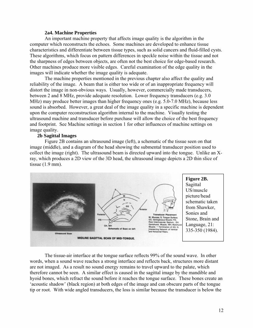
2b Sagittal Images Figure 2B contains an ultrasound image (left), a schematic of the tissue seen on that

image (middle), and a diagram of the head showing the submental transducer position used to collect the image (right). The ultrasound beam is directed upward into the tongue. Unlike an X-ray, which produces a 2D view of the 3D head, the ultrasound image depicts a 2D thin slice of tissue (1.9 mm).

Figure 2B. Sagittal US/muscle picture/head schematic taken from Shawker, Sonies and Stone, Brain and Language, 21: 335-350 (1984).

The tissue-air interface at the tongue surface reflects 99% of the sound wave. In other

words, when a sound wave reaches a strong interface and reflects back, structures more distant are not imaged. As a result no sound energy remains to travel upward to the palate, which therefore cannot be seen. A similar effect is caused in the sagittal image by the mandible and hyoid bones, which refract the sound before it reaches the tongue surface. These bones create an ‘acoustic shadow’ (black region) at both edges of the image and can obscure parts of the tongue tip or root. With wide angled transducers, the loss is similar because the transducer is below the

12

two bones. It is tempting to push the transducer upward into the tongue to see more of the tip. Unfortunately, this deforms the posterior tongue creating errors in its apparent shape. In addition to the tongue, some structures are sometimes visible in the image, but not reliably so.

2b1. Velum: When making a velar sound, the linguavelar contact allows the beam to pass into the velum and reflect back from the air above it, imaging the floor of the nasal cavity (see figure 2C).

Figure 2C Visible palate and velum in an ultrasound image.

2b2. Palate: If the tongue and transducer are held in constant alignment to each other, then the head is the reference, not the jaw, and it is valuable to track the palate and insert it on the image as a reference structure (see 3a. Transducer Stabilization for more details). During a swallow the tongue approximates the palate just after the bolus (item being swallowed) passes by. Therefore, palatal shape should be visible in a single frame or a series of frames in which a swallow is occurring (figure 2D). The palate is visible because the sound passes through the tongue and the mucosa below the palatine bone and reflects back from the bone itself. To get the best swallow image the subject should swallow dry and small amounts (3cc) of water. A water bolus can introduce some artefact, because air is ingested with the water and the water-to-air interface may be detected instead of the palate bone (see figure 2D). If possible, swallows with different size boluses should be collected and the best palate image used.

Figure 2D. Water bolus in front of mouth has air above it. Posterior tongue is visible.

13

2b3. The jaw: In an ultrasound image, the jaw cannot be seen directly, because it refracts the sound and creates an acoustic shadow (figure 2E). The shadow of the jaw is visible as a large conical shadow anterior to the tongue tip. The jaw’s shadow may obscure the tip of the tongue when the tongue is elevated, though we believe that no more than 1 cm of the tip is generally lost. If the transducer is positioned anteriorly enough, the lower lip is visible as a line that moves during speech. This is not an optimal way to measure lip motion, however. Inserting a video of the head (see below) provides much better lip formation.

hyoid shadow jaw shadowhyoid shadow jaw shadow

Figure 2E A sagittal image with hyoid and jaw shadows visible.

2b4. The hyoid bone: Like the jaw, the hyoid refracts the ultrasound and creates an

acoustic shadow (figure 2E). This shadow is narrower than the jaw’s. On rare occasions, some of the refracted sound will reach the transducer and the hyoid will appear as a bright spot, but the measurements are not reliable. Even when visible, hyoid shape cannot be demarcated. Reflections from the anterior edge cannot be differentiated from the lower edge. The shadow of the hyoid, on the other hand, can be seen quite clearly if the transducer is positioned posteriorly enough to capture it. Motion of the hyoid shadow can be interpreted as motion of the hyoid and can be used to identify stationary and moving portions of an event (e.g., swallowing). Note that the direction of hyoid motion is only partially recoverable, since forward motion cannot be distinguished from forward/upward motion.

2b5. Tongue extrema: pharynx and tip There are two reasons the tongue tip and root may not be visible on an ultrasound image.

The first is sound reflection and the second is sound refraction. The ultrasound ideally travels unimpeded through the tongue to the surface where about 99% reflects back from the air interface at the tongue surface. Due to this large reflection it is rare that structures beyond the strong tongue surface interface are imaged. Moreover, if an earlier interface causes considerable sound reflection, the tongue surface itself may not be imaged well. In the sagittal plane this is most obvious in two places. In the front of the mouth, the shadow cast by jaw and floor-of-the-mouth may obscure some of the tongue tip unless the tip is retracted or low (figure 2E) (Stone, 1990). In the back of the mouth, the hyoid bone obscures part of the posterior tongue surface (figure 2E). Typically, measurements of the tongue contour are best stopped at the hyoid shadow since it is difficult to distinguish tongue root from thyro-hyoid activity.

In addition to obscuration by acoustic shadows, the posterior tongue surface may be poorly imaged because of internal sound refraction. First, the tongue surface may be held at an angle

14

that is close to parallel to the beam, as in the case of /i/. In that case the sound refracts off the tongue surface and is poorly recovered by the transducer. Second, the tongue contains considerable fat, especially in the posterior regions. This fat, plus the multidirectional muscle fibres, cause refraction of the initial sound and the returning echo, reducing their strength and sometimes the clarity of an image.

2b6. Others: In the lower anterior portion of the image, the tendonous insertion of the medial head of genioglossus (GG) sometimes appears as a short bright line. It is tempting to use this as a reference point. Unfortunately, unlike the jaw, it is not a rigid body and even when visible cannot be assumed to have a fixed relationship to the tongue surface. Muscle fibres can sometimes be seen as well, in particular for GG (figure 2B).

2c. Coronal Images: Figure 2F depicts an ultrasound image in the coronal plane. Muscles can be seen, especially the bundled portion of GG in an anterior slice. A comparison between tongue dissection and ultrasound landmarks can be found in Shawker, Sonies, Stone, (1984).

Figure 2F. Coronal US/muscle picture/head schematic from Shawker, Sonies and Stone, Brain and Language, 21: 335-350 (1984).

2c1. Upper surface: As with the sagittal image, the upper surface of the tongue is

visible as the lower edge of the bright white line seen in the left image, and labeled (S) in the middle image. This line is the reflection from the air at the tongue surface. The tongue may appear unduly narrow in a coronal image. This is because an acoustic shadow resulting from the air beneath the lateral margins of the tongue may obscure the tongue’s lateral margins. This obscuration is most likely if the tongue is elevated enough to create a large air space. If the tongue is close to the long bones of the jaw, or there is enough saliva to transmit the sound wave, the edges of the tongue can be seen. In figure 2F the shadow begins at the line labelled (J), jaw inner aspect. The shadow is cast by the long bones of the jaw and the air medial to it. It is not possible to know how much of the lateral edges of the tongue are missing during speech, because apparent narrowing may be real. The tongue can compress medially to configure a particular phoneme or to elevate the tongue body. For an estimate of tongue width in rest position, the tongue width can be measured directly in the mouth and compared to the ultrasound measurement of width.

15

2c2. Palate and Jaw: Since the tongue approximates the palate in swallowing as the bolus passes by, palatal shape can be extracted from the full contact frame of a swallow, or by approximating the tongue to the palate in the region of the coronal scan. The jaw shadow is visible bilaterally (figure 2F) as well. Because the ultrasound beam hits the wide section of jaw’s long bone, and may include air, the bilateral shadows are large.

2c3. Transducer angles: The tongue is anisotropic, that is, not the same from front to back. It increases in width as new muscles enter (PG, SG and GH) and muscle fibres change in size and orientation. Videotaping the head from the side (discussed below) preserves the location of the coronal slice. It is useful to label the transducer angle in text directly on the image using degrees from vertical, or nominal labels, such as, cor1, cor2. 2d. Artefacts

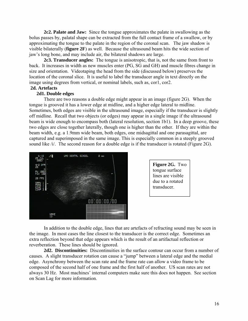
2d1. Double edges There are two reasons a double edge might appear in an image (figure 2G). When the

tongue is grooved it has a lower edge at midline, and a higher edge lateral to midline. Sometimes, both edges are visible in the ultrasound image, especially if the transducer is slightly off midline. Recall that two objects (or edges) may appear in a single image if the ultrasound beam is wide enough to encompass both (lateral resolution, section 1b1). In a deep groove, these two edges are close together laterally, though one is higher than the other. If they are within the beam width, e.g. a 1.9mm wide beam, both edges, one midsagittal and one parasagittal, are captured and superimposed in the same image. This is especially common in a steeply grooved sound like /i/. The second reason for a double edge is if the transducer is rotated (Figure 2G).

Figure 2G. Two tongue surface lines are visible due to a rotated transducer.

In addition to the double edge, lines that are artefacts of refracting sound may be seen in the image. In most cases the line closest to the transducer is the correct edge. Sometimes an extra reflection beyond that edge appears which is the result of an artifactual reflection or reverberation. These lines should be ignored.

2d2. Discontinuities: Discontinuities in the surface contour can occur from a number of causes. A slight transducer rotation can cause a “jump” between a lateral edge and the medial edge. Asynchrony between the scan rate and the frame rate can allow a video frame to be composed of the second half of one frame and the first half of another. US scan rates are not always 30 Hz. Most machines’ internal computers make sure this does not happen. See section on Scan Lag for more information.

16

2d3. Objects above the tongue surface: Other than the items mentioned above, reflections appearing above the tongue surface are artifacts and should be ignored.

2d4. Inconsistent transducer placement: A serious artifact is created by the erroneous belief that two tongue images are in the same orientation, when they are not. For example, if the transducer is held sagittally and rotated forward or backward, the display will not reflect the rotation. Similarly the display will not reflect rotation or translation from left-to-right. These errors and solutions are covered more fully under ‘manual transducer positioning’ below.

2d5. Artifacts in Swallowing: It is very difficult to take water into the mouth without including some air, whether the water is inserted using a straw, a syringe or a cup. Figure 2D shows a water bolus that is held in the mouth prior to swallowing. The posterior tongue appears as a curved line. The water-air interface produces a straight white line that is quite bright and should not be confused with the palate (figure 2C). The palate should be extracted from later images in the swallow when the tongue is at maximum height and the hyoid is elevated. For more information on applying ultrasound to the study of swallowing see Chi-Fishman (2005). 3. Transducer and Head Positioning

3a. Transducer Stabilization The goal of transducer positioning is to maintain intimate contact with the chin and accurate

beam direction, while ensuring no tissue depression (Stone and Davis, 1995). There are two methods for positioning the transducer under the chin, immobile (rigid) and mobile. When the transducer is rigid and the head is steady relative to it, tongue measurements are actually tongue-jaw measurements, and have the palate (i.e., skull) as the reference. This is because the image reference point, the transducer, is immobile relative to the head, so measurements made relative to the transducer are also relative to the head (or palate). In this case, tongue and jaw motion are not separate. Although tongue behavior can be subtracted from jaw motion using an additional instrument to measure jaw position, such as video, Optotrak or EMMA, bias will be introduced. That occurs because the tongue and jaw are not coupled equally along their length. The front of the tongue is more dependent upon jaw height than the back or root, so subtraction of complex tongue data from a single point on the jaw cannot be uniformly accurate.

With the second method, using a mobile transducer, tongue measurements are made with the jaw as reference. The transducer moves up and down with the jaw, thus tongue motion occurs relative to jaw motion and not head motion (cf Stone et al, 1988). These data are not aligned to the head and the apparent rotations and translations of the tongue are different from those that would be seen with a rigid transducer. A transducer held manually or moving on a spring-based platform, are both examples of mobile transducers and have a jaw-based reference. Moving transducer systems that also measure transducer, jaw and head position, can use these common external data points to mathematically correct in-plane errors of rotation or translation. (cf., Whalen, Iskarous, Tiede, Ostry, Lehnert-LeHoullier, & Hailey, D, in press, 2005). Corrections cannot be made, however, for out of plane motions, such as left-to-right translation or rotation due to transducer slippage, rotation, angulation, or head motion. When those problems occur, the tracking can only identify the error data for the investigator to delete.

Stone (1990) compared ultrasound data collected with a manually held mobile transducer (jaw reference), to the same dataset realigned to the palate (using an X-ray micro beam data set). The two data sets shared three common tongue pellets, which were used to align the tongue contours. The image sets looked very different (see Figure 3A). For additional information see Stone, 1990 and the Cervical Collar section of this paper. When interpreting tongue data it is important to identify whether the reference is the jaw or palate.

17

` 3a1. Rigid Transducer Placement

Head and Transducer Support System HA transducer that is rigidly locked into a fix

convenient because its position is known, is invariarigid transducer can be positioned using a rigid or jfloor-mount. With rigid transducer placement thereupward pressure may cause the transducer to deprehead motion will move the transducer to different rTransducer pressure can be minimized by using an upward pressure on the tissue (see next section). Wrelationship, only statistical measurements that are used (see below). The rigid transducer placement iimmobilized, creating a head-based coordinate syststatistics that require an unchanging spatial coordin

One successful system for rigidly positioninthe Head and Transducer Support System (HATS),fluoroscopy, and for which specifications are availaThis system is discussed further under head-holder

Other rigid transducers The transducer can be positioned rigidly be

attached to a chair or table. In that case, if the upwanalyses that are sensitive to translation and rotatio

Acoustic Standoff (see also X-ray Validat

Figure 3A Ultrasound tongue data aligned with the jaw (above) and the palate (below). Taken from Stone, 1990, JASA.

ATS ed position beneath the jaw is very nt and may be aligned with the head. The ointed holder attached to a chair, a table or a are two potential problems: invariant

ss the soft tissue of the jaw, and uncontrolled egions of the tongue during speech. acoustic standoff, which will eliminate ithout an unchanging head/transducer

insensitive to translation and rotation can be s advantageous when the head is em (shown in figure 3A). In that case, ate system can be used. g the transducer and immobilizing the head is which has been validated by x-ray video ble (Stone and Davis, 1995; Davis, 1999).

s.

neath the chin using a stable pole or a holder ard transducer force is minimized, statistical n can be used (see below). ion)

18

When the transducer is fixed, it acts as an obstacle to the jaw’s downward motion during speech. Since the point of transducer contact is the soft tissue under the tongue, this tissue is compressed proportionally to the size of the downward motion of the jaw. The amount of tissue compression varies depending on: 1. the position and length of the jaw muscles; 2. the degree of contraction of the muscle at that moment (increased contraction would create a harder muscle); 3. the surface area (per-square-inch relative to the area of the transducer); 4. the part of the muscle compressed (the middle is easier to compress than the ends); and 5. the position of the transducer.

There is some concern as to whether tissue compression alters apparent tongue behavior or produces artifactual motion in the image. Although strong upward pressure can cause as much as a 0.5cm shift in tongue surface (Stone and Davis, 1995), the acceptable amount of compression has not been effectively determined (see also X-ray Validation section). To prevent tissue compression, the transducer can be displaced from the skin using an acoustic standoff (Stone et al., 1988; Stone and Davis, 1995). An acoustic standoff is a soft, sonolucent pad (i.e., sound passes through it), developed to distance the transducer from the skin and allow ultrasound imaging of superficial structures that are closer to the surface than the transducer’s wavelength can image. Many standoffs are commercially available for this latter purpose; although these should be tested before purchase to be sure they are sufficiently compressible since many are too rigid to absorb the upward force of the transducer. A second method of displacing the transducer has been developed by Peng and colleagues (1996) called the cushion scanning technique (CST). In the CST, a latex bag filled with water is used as a cushion between the transducer and the chin. The head and transducer are in a fixed relationship to each other. They found more improved stability of swallowing measurements when using the CST than when using no standoff. Standoffs can degrade the ultrasound image, however, since some sound may be refracted. Some subjects have degraded image quality with standoff use.

3a2. Mobile Transducer Placement Hysteresis is the linearity with which the transducer tracks the jaw. When the jaw lowers

and rises, hysteresis describes whether the transducer moves synchronously. Typically such asynchrony is not constant or else it could be eliminated from consideration. The transducer begins moving downward more slowly than the jaw and reaches the bottom of the opening motion after the jaw. During the upward motion, the transducer again lags and is stopped in its upward motion by the cessation or reversal of jaw motion. Even if this has no effect on tissue compression, a temporal mismatch could result in time-based measurement errors of tongue motion (Stone et al., 1988). Hysteresis is a concern for manual positioning and for spring based mobile transducer housings as well. While experimenters should be aware of this problem, experience with manual positioning of the transducer, and the use of a constant-but-gentle upward force, can minimize this problem.

Manual positioning When the transducer is placed manually, some variability in spatial and temporal

positioning may be expected to occur as the hand moves up and down with the jaw. A concerted effort must be made to maintain the transducer at a constant position and pressure (relative to the jaw) during recording. One method for holding the transducer is shown in figure 3A. Place the thumb on the posterior edge of the ramus, and the forefinger anterior to the mandibular

19

symphysis. Hold the transducer between the middle and ring finger, in the sagittal or coronal direction, resting lightly against the underside of the chin. The entire hand and transducer move up and down with the jaw, as a unit. This technique measures tongue motion relative to the jaw (see figures 3B below).

Figure 3A. Ultrasound tongue data aligned with the jaw (above) and the palate (below). Taken from Stone, 1990, JASA

It is important to keep the orientation of the transducer constant and correct. To facilitate this, draw a vertical line with a permanent marker pen in the middle of the transducer in the direction of the midline of the beam. A similar line can be drawn, with a makeup pencil or non-permanent marker, on the midline of the subject’s chin. Place a mirror in front of the subject at an angle that allows the experimenter to see and align the subject’s head and the transducer. The mirror can be held by the subject or positioned on a table stand or wall. A final strategy can be used to stabilize tongue orientation across subjects and sessions. For example, if the transducer is held vertically for one subject and rotated back 15 degrees for another, any cross subject comparisons will be precluded because the data sets will have inconsistent measurement angles. To record a roughly comparable transducer angle across subjects, be sure that in the video image the shadows cast by the jaw and hyoid bones are equidistant from the 2 edges of the scan wedge (see figure 2E). This practice creates a consistent orientation for the tongue and serves to “normalize” the transducer position across subjects. More about this is discussed below (artefacts). The nature of some studies may require that this generally good practice be overruled, for example, in a swallowing study that is concerned primarily with hyoid motion.

Tracking transducer position When using a manually held transducer, there is occasionally some mistracking of the

tongue due to the motion of the experimenter's hand or the subject's head. In either case, the ultrasound beam may be rotated or translated out of the plane of interest for a half-second or more. At the typical ultrasound frame rate (30Hz) this mistracking lasts for 15+ frames. If the error is within the same plane, for example, if the head (or hand) slips, but stays within the midsagittal plane, the image can be rotated or translated back into the correct position. To do the correction would require that both the head and transducer be tracked by a point tracking device. However, if the slip is out of the plane, the correct data cannot be recovered because the time period is too long. In even a half second, tongue deformation is complex enough that prediction of missing shapes is unlikely. For longer periods the deformations are clearly not predictable.

20

3b. Head Stabilization An unstable head position leads to possible error due to head motion, leaning on the

transducer, or drift in position over time. An unrestricted head is convenient and possibly necessary for fieldwork. However, whenever possible the head should be restrained or immobilized, as this will markedly improve data reproducibility.

Holding the transducer in a known relationship relative to the head allows the tongue/jaw data to be aligned with the head (Stone and Davis, 1995). Complete immobilization of the head is sometimes accomplished using drastic measures. During brain surgery, the skull is immobilized by piercing it in three places with pins and locking the position. Immobile plugs can also be fitted to the subject’s ears, though not without discomfort. In MRI scanning, a custom facemask which locks the head to the MRI headrest, has been used to prevent head movement. These are unacceptable for ultrasound scanning due to discomfort or interference with speech.

There are several arguments for immobilizing the head. Head movement leads to inaccurate measurements, makes transducer position unreliable, and irregularizes contact between the transducer and chin. In the ideal ultrasound setup, the head and transducer are stabilized while the jaw moves freely. Thus, the transducer is in a known relationship with the head.

In some cases, such as fieldwork, it is very difficult to use an external head stabilization system. To maximally stabilize the subject’s head without an external device, methods used by dentists when making repeat cephalametric x-rays can be employed. Essentially, subjects must keep their eyes at exactly at eye level, with the pupil in the middle of the eye and look either into the reflected image of their own eyes in a mirror placed 3 ft. in front of them (Lundstrom and Lundstrom, 1992), or else focus on a point about 6 feet away (Moorrees, 1994). The pupil must be in the middle of the eye (Viazis, 1991).

It is tempting to allow the subject to look at the video monitor during data collection. This is fun for the subject and increases cooperation. However, it is recommended that the subject only be allowed to use this feedback before or after the data collection, but not during. The reason is threefold. First, the screen is probably not directly in front of the subject and the head follows the eyes toward the screen and rotates. Second, watching TV interrupts the focus on the task, as video is very distracting. Finally, biofeedback means that the speech is no longer natural. Tongue motion may be modified in response to the video information and such modifications cannot be predicted. There are a number of acceptable methods for holding the head and transducer in a constant and known relationship. Some methods stabilize the head and transducer using an external system, such as a dental chair or overhead structure, while others attach the transducer to a helmet or other head based system. Each has advantages and limitations. Head and transducer stabilization is an important and high priority investment in equipment that can be made as it improves the reliability and interpretability of the images.

3b1. Dental chair and headrest Although encircling the head is not the ideal method for stabilization (see Helmets, below), a circle combined with some local opposition or pressure points can provide quite good stabilization with normal subjects. Previous work indicates that a traditional dental chair with a two-cup head rest can be modified into a three point head rest by adding an arched plate that contacts the posterior head at a third point (see figure 3C). An eccentric, a metal cylinder that rotates outward, is attached to the headrest and a stabilization band is placed across the forehead

21

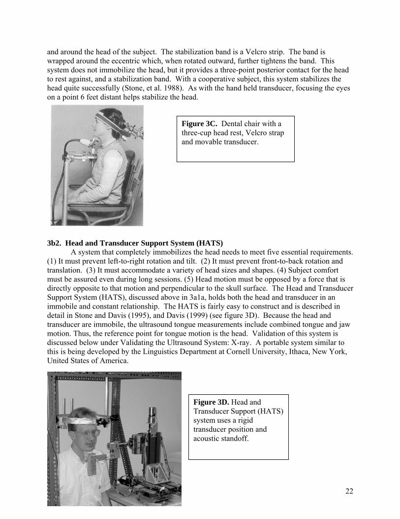
and around the head of the subject. The stabilization band is a Velcro strip. The band is wrapped around the eccentric which, when rotated outward, further tightens the band. This system does not immobilize the head, but it provides a three-point posterior contact for the head to rest against, and a stabilization band. With a cooperative subject, this system stabilizes the head quite successfully (Stone, et al. 1988). As with the hand held transducer, focusing the eyes on a point 6 feet distant helps stabilize the head.

3b2. Head and Transducer Support System (HATS)

A system that completely immobilizes the head needs to meet five essential requirements. (1) It must prevent left-to-right rotation and tilt. (2) It must prevent front-to-back rotation and translation. (3) It must accommodate a variety of head sizes and shapes. (4) Subject comfort must be assured even during long sessions. (5) Head motion must be opposed by a force that is directly opposite to that motion and perpendicular to the skull surface. The Head and Transducer Support System (HATS), discussed above in 3a1a, holds both the head and transducer in an immobile and constant relationship. The HATS is fairly easy to construct and is described in detail in Stone and Davis (1995), and Davis (1999) (see figure 3D). Because the head and transducer are immobile, the ultrasound tongue measurements include combined tongue and jaw motion. Thus, the reference point for tongue motion is the head. Validation of this system is discussed below under Validating the Ultrasound System: X-ray. A portable system similar to this is being developed by the Linguistics Department at Cornell University, Ithaca, New York, United States of America.

Figure 3D. Head and Transducer Support (HATS) system uses a rigid transducer position and acoustic standoff.

Figure 3C. Dental chair with a three-cup head rest, Velcro strap and movable transducer.

22

3b3. Helmet The apparently ideal solution to keeping the head and transducer in constant relationship

is to attach the transducer to a helmet. This can be done, but not in an obvious manner. In previous work, two different helmet designs met with poor success. The first, a US-football helmet (Riddell), contained expandable regions that could be filled with air or water. Even without molding to the subject's head, the helmet was quite tight. The most important problem was that with such a large helmet there was not enough usable space left below it for the transducer. In addition, the head was able to move within the helmet. Other unexpected problems were that the helmet was very claustrophobic, reduced hearing and restricted vision. A small but important problem was that it irreparably flattened the subject’s hair, making it unacceptable to subjects during their workday. The second helmet was a lacrosse helmet filled with expanding foam. This was a smaller, more comfortable helmet in which the foam tightened the space around the head and moved with the head. However, even with considerable foam and an uncomfortably tight fit, the head was able to rotate within the helmet. What became clear from these endeavors was that any device encircling the head would not prevent some rotation. This can be demonstrated by pushing against the forehead with the index finger and rotating the head left and right. The skin remains steady beneath the finger, but the skull moves. The skull moves because it is not coupled tightly to the skin. As a result, irrespective of how hard one pushes the forehead or squeezes the head with an encircling ring, the head will always be able to rotate.

In a helmet, the directions of rotation with the largest error are front-to-back and left-to-right rotation. One way to modify a helmet to prevent rotation would be to cut holes in it on either side and in the back, and insert clamps that locally approximate the head and prevent motion. This arrangement would then be similar to the padded clamps in the HATS system. Such a system would prevent head rotation within the helmet, while allowing the transducer to attach to it, and thus facilitate head/transducer alignment. This helmet modification is being developed at Queen Margaret University College in Edinburgh, Scotland.

3b4. Cervical Collar Another portable method for supporting the head and transducer is a cervical collar. A number of these are available commercially at low cost. They are typically made of plastic and several have fairly large openings in the front (see figure 3E). With minor modifications the openthe opening (Stone, Sutton, Partharestricts jaw motion, however, thu1971). Nonetheless, further modif4. Validation and Calibration

4a. Anatomy

Figure 3E The ultrasound transducer is below the neck, attached to the collar. A microphone is positioned in front of the subject’s mouth for simultaneous audio recording

ing can be enlarged and a transducer positioned rigidly within sarathy, Prince, Li, Kambhamettu, 2002). The cervical collar s modifying tongue behavior (cf. Lindblom and Sundberg, ication might overcome that restriction and is worth exploring.

23

An ideal way to validate the anatomy seen on ultrasound is to scan a cadaverous tongue and then dissect it. Anatomical validation was done by Shawker et al. (1984), among others. An excised human tongue, including hyoid and epiglottis was obtained 12 hours after death. The tongue was submerged in a water bath and scanned in the midsagittal and coronal planes. After scanning, a dissection was performed. The orientation and sizes of several structures were compared in situ and in the ultrasound scan, including genioglossus m., mucosa, and fat. They were found to be the same. In addition, the hyoid bone produced the same shadow on the scan as predicted clinically.

4b. X-ray Every ultrasound data collection system needs to be validated to be sure that it does not affect the tongue data adversely. The earliest validation of ultrasound was a comparison of the tongue surface from an ultrasound image with one from a simultaneous x-ray (Sonies, et al. 1981). Similarly, a circular-band head holder and manually held transducer were validated by comparing strain gauge motion of the mandible with the motion of the transducer to test for hysteresis (Stone, et al. 1988). See also 3a1c. Acoustic Standoffs. An x-ray validation study of the HATS system yielded good results because it used an acoustic standoff to absorb upward transducer pressure. The standoff was a ¾” (2cm) thick gelatinous slab made of polymerized mineral oil (Kitecko, 3M Co.). The sound // was spoken in /s/ and /t/ context and the tongue surface was measured both with the transducer in place and with it removed. When the ultrasound measurements were compared with X-ray measurements the tongue contour differences were found to be less than 0.2mm, which is within the measurement error of 0.5mm.

4c. Phantoms An ultrasound phantom, or ground truth, can be used to determine the accuracy of a specific

ultrasound machine. Ultrasound phantoms are scannable objects that contain within them points, lines, and objects of known dimensions with which to test the accuracy of the ultrasound transducer and machine. They are commercially available and also owned by most radiology departments doing clinical ultrasound studies. 5. Data Recording

5.a. Sample recording set up. There are many ways to configure an ultrasound laboratory. The current Vocal Tract Visualization Laboratory at the University of Maryland is one such example (see figure 5A); its physical layout is the framework for the instruments discussed in this section.

Figure 5A. Vocal Tract Visualization Lab schematic

24

5.b. Much of the recording set up is covered in the sections above. Before the data

recording begins, it is assumed that the lab has been configured and determinations made about head and transducer positioning, subject selection, speech materials, and imaging planes. The subject is seated in a comfortable chair and immobilized as much as possible. The subject should not extend her/his chin unnaturally to accommodate the transducer as such a position is difficult to maintain, and encourages drift over time. Head and back position should be as natural and comfortable as possible. Within those limits, however, if the subject is angled slightly forward (from the waist or hips), it is often easier to get the transducer under the chin without the transducer cord hitting the subject in the chest, in addition, the hyoid and jaw are slightly farther apart increasing the visible portion of the tongue surface. The jaw and hyoid shadows should be positioned at equal distances from the two edges of the image (figures 2C and 5B).

c. Additional data in the image

s or greater, contain a large region of unused space. If the r

ted

e insertion of timing information on the image serves two purpos use the

ry

ell.

Figure 5B. Ultrasound image with inserted clock, audio wave and head.

5Ultrasound images, at 640 x 480 pixel

ecording setup permits, additional data can and should be inserted into the image for future reference. Some of this material is essential and some will be helpful. They are presenfrom most to least important.

5c1. Video timer: Thes. It marks each frame with a unique number (figure 5B). This is important beca

tongue moves continuously in the ultrasound image. The unique number marks the image so that when scrolling through a sequence it is possible to return to a specific image. The timing information also facilitates the measurement of duration since the elapsed time between two frames can be calculated easily. The video signal is channeled through the timer and a digitalclock is inserted onto the image. The clock needs to display hundredths of a second so that eveframe (30 Hz) will have a unique number. Without unique frame markers specific frames of interest are very difficult to find a second time. Some VCR’s can insert numbers on the imageduring playback, but these are rarely permanent. Direct computer capture can alleviate this somewhat because the computer frames are numbered in sequence. However, the face of theimage will not have timing information when opened in isolation. It is also very important to check the AV synchrony as many analog/digital devices do not synchronize the two signals w

25

In fact, audio and video are often synchronized only to within one second, leaving open the possibility of AV misalignment by as much as 30 frames.

5c2. Alphabet characters: Subject and task information ideally should be typed in as the data are collected. Typing the word as the subject starts to speak, or typing the item first and then typing an asterisk as the subject begins, can make it much easier to find the item later when scrolling through frames in fast forward or reverse. To increase the speed of typing and data collection, alphabetical information can be continuously added and left on the screen until the typing area gets full. Non-erasure also makes the session history visible throughout the data set (see figure 5B).

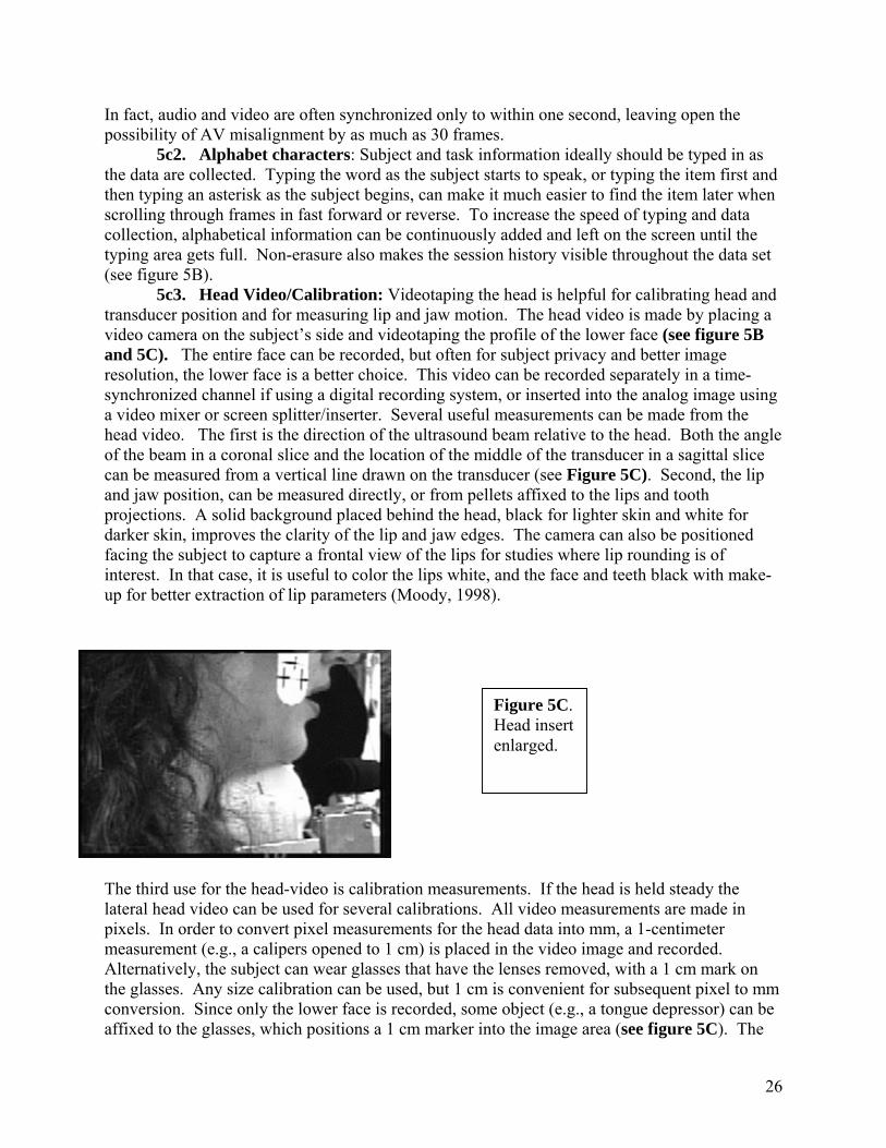
5c3. Head Video/Calibration: Videotaping the head is helpful for calibrating head and transducer position and for measuring lip and jaw motion. The head video is made by placing a video camera on the subject’s side and videotaping the profile of the lower face (see figure 5B and 5C). The entire face can be recorded, but often for subject privacy and better image resolution, the lower face is a better choice. This video can be recorded separately in a time-synchronized channel if using a digital recording system, or inserted into the analog image using a video mixer or screen splitter/inserter. Several useful measurements can be made from the head video. The first is the direction of the ultrasound beam relative to the head. Both the angle of the beam in a coronal slice and the location of the middle of the transducer in a sagittal slice can be measured from a vertical line drawn on the transducer (see Figure 5C). Second, the lip and jaw position, can be measured directly, or from pellets affixed to the lips and tooth projections. A solid background placed behind the head, black for lighter skin and white for darker skin, improves the clarity of the lip and jaw edges. The camera can also be positioned facing the subject to capture a frontal view of the lips for studies where lip rounding is of interest. In that case, it is useful to color the lips white, and the face and teeth black with make-up for better extraction of lip parameters (Moody, 1998).

Figure 5C. Head insert enlarged.

The third use for the head-video is calibration measurements. If the head is held steady the lateral head video can be used for several calibrations. All video measurements are made in pixels. In order to convert pixel measurements for the head data into mm, a 1-centimeter measurement (e.g., a calipers opened to 1 cm) is placed in the video image and recorded. Alternatively, the subject can wear glasses that have the lenses removed, with a 1 cm mark on the glasses. Any size calibration can be used, but 1 cm is convenient for subsequent pixel to mm conversion. Since only the lower face is recorded, some object (e.g., a tongue depressor) can be affixed to the glasses, which positions a 1 cm marker into the image area (see figure 5C). The

26

marks on the tongue depressor in figure 5C represent head position and can be used as a reference for lip and jaw motion. Additional calibration measures can be made, such as the occlusal plane, which can be extracted by having the subject bite with back molars on a tongue depressor (see figure 5C). If the subject puts his/her tongue against the lower edge of the depressor, the ultrasound image will show the plane. This plane can be compared to the tongue surfaces in the ultrasound image.

5c4. Audio Signal: The speech wave can also be displayed on an oscilloscope, videotaped and inserted on the image. This is useful for extracting acoustic landmarks such as voice onset and manner of production; then measuring the images without the audio because each image will contain a tongue shape and the simultaneous audio wave (±16 ms), see figure 5B. In cases where the audio and video are displayed synchronously during analysis, this is less important because the actual audio signal will be available for landmark corroboration. The speech wave and head video can be inserted on the image using a video mixer and a screen splitter/inserter (figure 5A).

5d. Normalizing across recording sessions and subjects To be able to compare data from multiple sessions of the same subject, it would be helpful to reposition the subject in the same place. One solution is to use a bite mold to reposition the head in its previous position. A bite mold (figure 5D) is created by taking an impression and making a cast of the subjects bite. When the subject bites down on the mold his/her teeth are realigned to the original position placing the jaw and head in the same relationship as previously. A bite mold was created for a single subject. Figure 5D shows the subject in the HATS system with the mold fitted into position after the subject was positioned comfortably in HATS. To test the system the head clamps were loosened, the chair moved back and the subject removed herself from the system for a 15-minute break. She then returned and was repositioned in the HATS system while biting on the unmoved bite mold. By moving the chair and head clamps, a concerted attempt was made to reposition her exactly in the earlier position. Figure 5E indicates that although the teeth are in the same position, the neck and shoulders are not, which creates a different jaw/tongue/hyoid orientation. Additional variability can be expected when not using a head-holder. This occurs because the upper body has many degrees of freedom. Placing the transducer in the previous position, therefore, may not guarantee identical data sets across sessions. An alternative method for subject normalization is careful positioning of the jaw and hyoid shadows equidistant from the two edges of the image (see section 5a), followed by statistical (rigid body) alignment of the extracted tongue contours.

Figure 5D. Repositioning the head with a bite mold.

27

Figure 5E. The teeth are in the same place, but the neck is not.

Prior to statistical analysis, extracted tongue contours can be processed mathematically, prior to statistical analysis, to align data from multiple sessions and subjects. This statistical pre-processing consists of overlaying all the contours onto a common coordinate system (across sessions and speakers). Within a session contours are overlaid and extended or cut to the same length. The process is repeated across sessions and subjects. The contours are shifted to a common x and y range and truncated to a common length. Full details and discussions of numerous methods for statistical pre-processing are found in Slud, Stone, Smith, and Goldstein (2002). Normalization of pellet placement across subjects is discussed in the section on Pellets, below. 6. Ultrasound Data Analysis and Statistical Representation Once the ultrasound images are digitised, the tongue surface contours need to be measured. A challenge in measuring ultrasound images is the lack of a physiological reference. Although the tongue contours are clearly visible, there are no hard structure references, making it difficult to determine an exact position for the tongue in the vocal tract. The head and transducer holders help overcome this problem, as do some of the analyses discussed below.

Extracted tongue contours are very high dimensional. A single contour may be represented by as many as 100 points. These points all move during speech, some in a more correlated manner than others. It is easy to see local and global components of the motion. It is a challenge, however, to identify and quantify functionally important features. In order to get more information out of the extracted tongue contours it is useful to reduce their dimensionality. A reduction in dimensionality also is essential for a statistical examination of task effects or speaker effects on tongue shapes. Further, 2D contours can be reduced prior to 3D reconstruction. There are a number of quantities that can reduce the tongue’s dimensionality globally or locally. A short summary of each is presented below along with and a reference to a paper providing more detail. The basic ultrasound data reduction software used in the VTV lab is displayed in the schematic below in figure 6A. The figure shows the data analysis sequence. Column 1 shows tongue surface contours (red dots), which are extracted from each frame in a sequence (for more details, see Li et al, 2005a.). The changes in tongue shape during speech or swallowing are displayed in column 2 as time-motion displays, either as a traditional waterfall (bottom) or as an x,y,t surface (top). Column 4 shows two x,y,t surfaces overlaid and ready for statistical comparison. (for more details see Parthasarathy, Prince, Stone, 2005).

28

Waterfall Display

Tongue Surface

Orientation

Contour Extraction

x, y, t Surface

/g//l/

/i/

Overlay twox, y, t surfaces

Surf 1 = whiteSurf 2 = color

321

C1d

back

Waterfall Display

Tongue Surface

Orientation

Contour Extraction

x, y, t Surface

/g//l/

/i//g/

/l//i/

Overlay twox, y, t surfaces

Surf 1 = whiteSurf 2 = color

321

C1d

back

6a. Image Quality It is important when digitising ultrasound images to be sure the system does not unduly degrade the images. Uncompressed images, such as tiff or AVI movies, are of higher quality than compressed, but take up more storage space (300-1200KB per frame). Compressed images take up a fraction of the space, but are often of poorer quality. Lossless jpegs, such as LZW compression at 70% original size, are of high quality and small in size (24-40KB). Figure 6B shows 3 images directly digitised and stored by different commercially available systems. The quality differences are self-evident, particularly when reading the text at left. Before selecting a computer system, careful observation of image quality will improve the validity of subsequent measurement and ease of interpretation.

at

Figure 6B. Images with different compression formats. GIF, compressed JPG, less compressed JPG.

6b. Extracting tongue contours

6b1. Measurement Error: There are two sources of measurement error in ultrasound nalysis: ultrasound instrument ‘noise’ and human imprecision. Instrument noise includes ransducer placement inaccuracies, image resolution and reconstruction inaccuracies, all of

29

which determine how precisely an object is represented in the image. These effects are discussed in section 1a1: Ultrasound Beam Properties.

Once image quality and resolution are optimised for the instrument, human measurement error can be reduced with training to within 1 pixel. One pixel typically represents 0.25-0.5mm depending on the depth setting used and the machine. This value, calculated from the cm scale on the ultrasound image, varies with depth setting. Measurement error was recorded in several previous studies. Stone et al. (1983) found that for two judges, within-judge reliability was r=0.96 and r=0.99, respectively; the between-judge reliability was r=0.99. Maximum measurement error was found to be 0.7mm. Stone et al (1988) found measurement error to be 1-pixel (0.49mm). With a measurement error of 1 pixel, a better spatial resolution in the image, that is, fewer mm per pixel, will reduce measurement error in mm. Shallower depth settings decrease the number of mm per pixel.

6b2. Using a superimposed grid A simpler method of edge extraction is to measure several points of interest on the tongue

surface. This method does not require an edge detection program and allows extraction of data at locations-of-interest on the tongue surface. The method also reduces the tongue’s dimensionality by representing it as a few points. The points can be selected in an xy coordinate space (Cartesian), or a theta, radius, coordinate space (Polar). The latter examines displacement toward and away from a single point within or below the tongue rather than up/down and front/back motion (see figure 6C). Although the problem of referencing the tongue is not solved by a superimposed grid, it enables identification and measurement of the tongue using the transducer as a reference point (cf. Stone et al., 1983). This method relies on the assumption that during data collection transducer position was reliable and can serve as a reference. Digital edge extraction allows the imposition of a radial grid on the extracted contour by positioning the data points in a polar coordinate space. These displacement data can be used in statistical analyses of local displacement, local curvature, tongue segmentation and graphic representation of the image. Statistical analyses are discussed below.

Figure 6C. Grid superimposed on ultrasound image Stone et al, 1983.

6b3. Semi-Automatic Edge Extraction: Manual extraction of selected points is tedious

and time consuming especially if used in time-motion sequences of 30 frames per second. Alternatively, selecting only a few points using an overlaid grid, means that features of interest may be overlooked if they occur between the points. Automatic edge extraction and tracking that allows fast accurate measurements of tongue contours would be ideal for ultrasound tongue analysis. Unfortunately, because the ultrasound image is very noisy, the brightest edge may not be the important edge and it has been found that even automatic systems need to be supervised by a human experimenter to be sure that the selected edges are accurate. Even with this limitation, semi-automatically extracted data are far superior to manual processes in terms of

30

time and convenience, are equally accurate, and provide large quantities of data. As a result of the increased data more complex theoretical issues can be studied. For additional information of edge detection see Iskarous (2005).

For those who do not use an automatic edge extraction and tracking system, the VTV lab extends to users, without cost, Edgetrak, a semi-automatic program that extracts tongue contours in a sequence of ultrasound images. This custom software (Li, et al, 2003, 2005a), and directions are available from the VTV website, http://speech.umaryland.edu/software. The output data points are xy coordinate points stored in an ascii (text) table that can be opened in Excel and other data analysis programs.

6c. Statistics for Manual Transducer Placement Since manual transducer positioning may be unstable over time, it is desirable to seek

tongue shape parameters, which have little or no dependence on absolute position. (See Section 3a2b). There are several mathematical quantities that are unaffected by this motion. These include averaging, curvature and polynomial functions among others.

6c1. Averaging Normal within-subject variability means that any single repetition of a speech task may

not be an ideal exemplar of that task. In addition, the ultrasound frame rate is too slow to perfectly capture rapid motion even if the repetitions are identical. For both these reasons, an average contour is a better choice for a representative exemplar than a single contour. A tongue surface contour is actually a set of xy-points. Recall that the xy values are arbitrary points. However, in order to average a set of contours, the x-values must be the same for all contours. This is accomplished by linear interpolation, which creates additional points in each contour; then the new contours are re-sampled at identical x-values, whose corresponding y-values are averaged. (Morrish, Stone, Shawker, Sonies, 1985, Li et al, 2005b, Parthasarathy et al 2005. Standard deviations can also be computed, but one must be aware that variability has multiple sources, including physiological variability in tongue position, measurement error and instrumental error.

6c2. Curvature When the ultrasound transducer is placed manually, some position errors may be

expected. When that variability cannot be corrected it is desirable to seek tongue shape parameters that have a weak dependence on position. These measurements are useful for data collected with a rigid transducer and restrained head as well.

A shape parameter with a weak dependence on position is curvature. The parameter ‘curvature’ is a quantifiable feature, which preserves small-scale elements of tongue shape and makes no assumptions about overall shape. Because curvature calculations are based on local slope and degree of concavity/convexity, curvature at a point on a curve is independent of translation and rotation. Rotation is the motion of a body about an axis. Translation is the directional motion of a body independent of rotation. Both of these are rigid body features and are independent of deformation.

Conceptually, curvature can be explained by the diagram in figure 6D. Any three points (e.g. points A, B and C) can be conceived of as lying on the circumference of a circle. That circle will have a radius, the inverse of which represents the curvature of the circle passing through those three points. In an extracted edge, the surface of the tongue is a series of points (bottom of figure 6D). In such a series, every set of three points yields a curvature value, which is the inverse of the radius of the circle passing through them. Three points that lie along a straight line have a curvature of zero, since their concavity is zero and this becomes the

31

numerator of the curvature equation (Morrish, Stone, Sonies, Kurtz, Shawker, 1984; Stone, Morrish, Sonies, Shawker, 1987).

Given a sequence of three points, x1y1, x2y2, and xbe calculated from the equation K(x) = ______f ”(x)______ (1 + (f ’ (x) ) 2) 3This equation is rewritten as a series of steps for usParthasarathy).

K(x2,y2) = f2" / [1+(f2')^2]^(3/2) Where

f2'= ((h2^2*y3)+(h3^2-h2^2)*y2-(h3^2*y1f2" = (h3*y1 - (h2+h3)*y2 + h2*y3) / (1/2)

and h2 = x2 - x1 h3 = x3 - x2 When using a manually positioned transduc

reference structures are not necessary. Vertical dishorizontal displacement and transducer rotation affrespect to the x-axis not their magnitudes. In additicurvature provides a simplified representation of tovalues used in the computation of curvature is criticdifference formulas will be inaccurate. If points arbe amplified in the second derivative giving spurioinaccuracies.

A study examining tongue curvature in fouret al, 1987), determined that a point separation of astudy found that location of maximum curvature anlower tongue produced a more posterior max-curvaposterior to max-displacement.

6c3. Curve Fitting (Polynomial functionsCurve fits, or polynomial functions are wea

can be used with manual transducer placements. A

Figure 6D. Curvature diagram. A circle can be fitted to any three points. From Morrish et al, 1987

3y3, curvature of the middle point, x2y2, can

__ /2

e in Excel or Matlab (Provided by V.

))/h2*h3*(h3+h2) *h2*h3*(h2+h3)

er, curvature is an excellent statistic, because placement does not affect curvature; ect only the location of curvature values with on, the location and magnitude of maximum ngue shape. However, the distance between x al. If the distances are too large, the finite

e chosen too closely together, noise errors will usly high curvatures to measurement

subjects for the vowels /ae, a, i, u, o/ (Stone bout 8 mm was optimal for the study. The d maximum displacement were correlated. A ture, and maximum curvature was always

) kly dependent on tongue position, and as such ny degree of polynomial can be fit to the

32

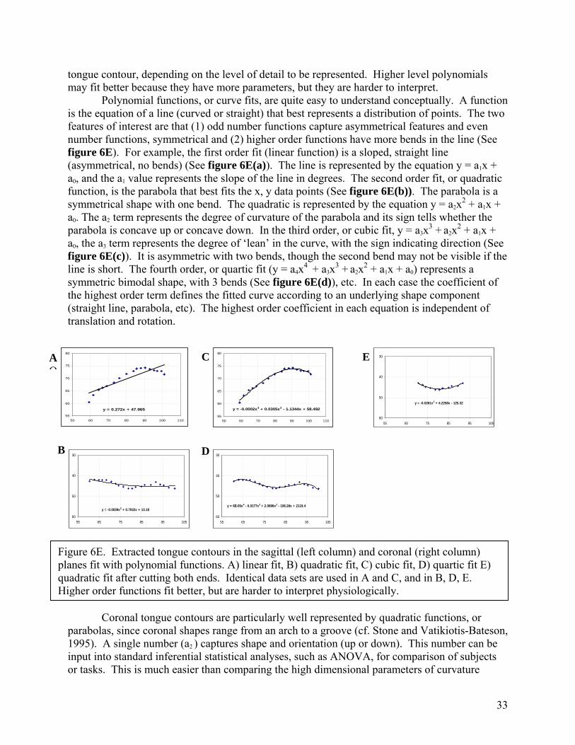
tongue contour, depending on the level of detail to be represented. Higher level polynomials may fit better because they have more parameters, but they are harder to interpret.

Polynomial functions, or curve fits, are quite easy to understand conceptually. A function is the equation of a line (curved or straight) that best represents a distribution of points. The two features of interest are that (1) odd number functions capture asymmetrical features and even number functions, symmetrical and (2) higher order functions have more bends in the line (See figure 6E). For example, the first order fit (linear function) is a sloped, straight line (asymmetrical, no bends) (See figure 6E(a)). The line is represented by the equation y = a1x + a0, and the a1 value represents the slope of the line in degrees. The second order fit, or quadratic function, is the parabola that best fits the x, y data points (See figure 6E(b)). The parabola is a symmetrical shape with one bend. The quadratic is represented by the equation y = a2x2 + a1x + a0. The a2 term represents the degree of curvature of the parabola and its sign tells whether the parabola is concave up or concave down. In the third order, or cubic fit, y = a3x3 + a2x2 + a1x + a0, the a3 term represents the degree of ‘lean’ in the curve, with the sign indicating direction (See figure 6E(c)). It is asymmetric with two bends, though the second bend may not be visible if the line is short. The fourth order, or quartic fit (y = a4x4 + a3x3 + a2x2 + a1x + a0) represents a symmetric bimodal shape, with 3 bends (See figure 6E(d)), etc. In each case the coefficient of the highest order term defines the fitted curve according to an underlying shape component (straight line, parabola, etc). The highest order coefficient in each equation is independent of translation and rotation. )

y = 0.272x + 47.96555

60

65

70

75

80

50 60 70 80 90 100 110

C E

y = -0.0261x2 + 4.2258x - 125.32

30

40

50

6055 65 75 85 95 105

y = -0.0002x3 + 0.0305x2 - 1.1344x + 58.492

55

60

65

70

75

80

50 60 70 80 90 100 110

B

y = 6E-05x4 - 0.0177x3 + 2.0896x2 - 108.28x + 2119.4

30

40

50

6055 65 75 85 95 105

D

y = -0.0039x2 + 0.7032x + 13.18

30

40

50

6055 65 75 85 95 105

Figure 6E. Extracted tongue contours in the sagittal (left column) and coronal (right column) planes fit with polynomial functions. A) linear fit, B) quadratic fit, C) cubic fit, D) quartic fit E)quadratic fit after cutting both ends. Identical data sets are used in A and C, and in B, D, E. Higher order functions fit better, but are harder to interpret physiologically.

A O

Coronal tongue contours are particularly well represented by quadratic functions, or

parabolas, since coronal shapes range from an arch to a groove (cf. Stone and Vatikiotis-Bateson, 1995). A single number (a2 ) captures shape and orientation (up or down). This number can be input into standard inferential statistical analyses, such as ANOVA, for comparison of subjects or tasks. This is much easier than comparing the high dimensional parameters of curvature

33

signatures or averages, which require a different type of analysis (discussed in section 6e). Fourth order polynomials have also been fit to coronal tongue contours, and in fact are often closer to the true shapes (figure 6E(b)vs 6E(d)), however, they are harder to interpret (Stone and Lele, 1992). An alternative approach is to fit a quadratic to the inner part of the tongue contour (figure 6E(e)).

Midsagittal ultrasound tongue contours have also been represented with polynomial functions. Morrish et al. (1984; 1985) found that second and third order curve fits reliably represented midsagittal tongue shape and distinguished among the four extreme vowels. In other, unpublished work, however, third order fits were found to be very sensitive to line length. This effect is seen in figure 6E(e), in which the coronal contour from 6E(b)+(d) has been cut at both ends yielding an entirely different (in this case better) quadratic fit. This effect, however, means that changes in sagittal contour length, which are due to visibility of the tongue tip or root and do not change line shape, will alter the a3 term. Thus the polynomial function is not the best way to capture sagittal shape. However, high order functions (6-9th order) fit contours very well and are an excellent way to reduce noise. Morrish et al. (1984) found that calculating curvature from fitted curves was less noisy than the using original curves.

6d. Principal Components Analysis If several conditions are met: (1) the transducer is placed in a fixed, known position on

the subject, and (2) the subject’s head is stabilized relative to the transducer, additional statistical quantities are available for data analysis. One of these methods is Principal Components Analysis (PCA). PCA is a method of reducing the dimensionality of tongue contours and can be used to extract and depict contour features in a data set. The data set can contain multiple tasks, sessions and even subjects. The data set-up for a PC analysis has specific requirements, which are explained in detail in Slud et al (2003). The PCA technique itself is explained very well in The Mismeasure of Man (Norton, 1996) by Stephen Jay Gould: “Factor analysis [also PCA] is a mathematical technique for reducing a complex system of correlations into fewer dimensions. It works, literally, by factoring a matrix, usually a matrix of correlation coefficients. (Remember the high-school algebra exercise called “factoring,” where you simplified horrendous expressions by removing common multipliers of all terms?) Geometrically, the process of factoring amounts to placing axes through a football of points. In the100-dimensional case, we are not likely to recover enough information on a single line down the hyperfootball’s long axis—a line called the first principal component. We will need additional axes. By convention, we represent the second dimension by a line perpendicular to the first principal component. This second axis, or second principal component, is defined as the line that resolves more of the remaining variation than any other line that could be drawn perpendicular to the first principal component. If, for example, the hyperfootball were squashed flat like a flounder, the first principal component would run through the middle, head to tail, and the second also through the middle, but from side to side. Subsequent lines would be perpendicular to all previous axes, and would resolve a steadily decreasing amount of variation. We might find that five principal components resolve almost all the variation in our hyperfootball—that is, the hyperfootball drawn in 5 dimensions looks sufficiently like the original to satisfy us, just as a pizza or a flounder drawn in two dimensions may express all the information we need, even though both original objects contain three dimensions. If we elect to stop at 5 dimensions, we may achieve a considerable simplification at the acceptable price of minimal loss of information. We can grasp the 5 dimensions conceptually; we may even be able to interpret biologically.” (Gould, 1981, p. 245-6) Two very important aspects of PCA are often given inadequate attention. The first is that PCs are not theoretically based; they have no physical meaning. PCA is a statistical method that is entirely data driven. A different data set may produce entirely different PCs. Even a slightly different data set will produce slightly different PCs. As with correlation, the theory comes from outside, not from within the data distribution. In speech research, where PCA is often applied to tongue contour data, resulting PC shapes may be interpreted physiologically. This has happened

34

with ‘front-raising’ and ‘back-raising’ whose shapes emerge from vowel data in various studies (cf. Harshman, Ladefoged, Goldstein, 1977; Jackson, 1988b, Stone and Lundberg, 1996). In such a case, there may be some reality to the underlying shapes. However, PC shapes are arbitrary and PCs with no interpretable shape at all are equally valid because the function of the PC is to mathematically, not theoretically, represent the variance in the data set. In other words, PC’s do not extract underlying theoretical features.

The second often-overlooked feature is that PCA not only represents tongue shapes, it offers a means of comparison between groups. PCA includes all the groups being compared: subjects, tasks, sessions, etc. As such, the loading of various groups on the PC’s indicates group differences, though not necessarily the statistical significance of those differences. Harshman, et al (1977) and Hoole (1999) used PCA analysis (PARAFAC) to extract some subject information. Statistical analyses can be performed on single PCs or a combination of several (cf. Slud et al., 2002).

PCA has been used successfully to represent midsagittal tongue contours for vowels (cf., Jackson 1988b, Maeda 1990,) and to separate subject from. vowel variability (Harshman et al., 1977; Hoole, 1999). Coronal shapes also have been represented using PCA. Stone, Goldstein and Zhang (1997) examined 11 vowels in 2 consonant contexts for a single subject and found that two PCs explained 93% of the variance. The representations of the tongue shapes as linear combinations of the first two PCs were consistent with traditional phonetically based groupings. Later work extended that study by examining multiple subjects and sessions (Slud et al., 2002). That study found three PC’s that covered the same range of shapes as the first study, and again explained 90% or more of the data for this much more diverse data set. The PC shapes were changed somewhat, however, showing that underlying universal features are not well extracted by PCA.

6e. Comparative Measures and Display Once the tongue contour is quantified satisfactorily, it is of interest to compare across groups

to study differences between tasks or subjects. Any qualitative measurements that reduce the tongue parameter of interest to a single value can be used in standard parametric or non-parametric comparative statistics, such as ANOVA or correlations. In many quantification schemes, however, the final data set is high dimensional, for example, individual contours, averaged contours, slope and curvature signatures, or comparisons of entire curve fit equations.

6e1. Surfaces: A convenient method of visualizing the raw or averaged data set is a time-motion display of a sequence of contours. A traditional time-motion waterfall displays the contours as a sequence making deformation visible (see figure 6A). A tool that builds on the traditional waterfall display is a program called Surfaces, developed to display a series of contours over time as a single 3D entity; the x, y points from each contour and the t (time) values for each contour are displayed as a 3D surface (see figure 6A and 6F). The Surfaces program displays individual contour sequences, calculates averages and variances for multiple repetitions, and compares x,y,t surfaces. Tongue shape comparisons can be done globally, using L1 norm and L2 norm or RMS difference comparisons, or locally, by subtracting the distance between specified tongue segments. Surfaces are discussed in detail in Parthasarathy et al. (2005), and the program is available without cost from the VTV lab at http://speech.umaryland.edu/software.

35

Figure 6F: Sequence of midsagittal contours for the word “golly” displayed using the SURFACES program. Tongue tip is on the right.

6e2. Ln norms and average differences.

To globally compare the difference between two contours there exist error metrics, which essentially look at the area between the two curves. They include summary differences (the Ln norm family) and average differences (average and root-mean-square (RMS)). The disadvantage of average measures is that they are influenced by a few extreme values. The advantage is that results can be compared among data sets with different Ns, because the average units are comparable in magnitude to those of the tokens (unlike sums). Both type calculations require an equal number of data points in the comparison curves, which can be accomplished by prior cutting, extending, or shifting of the curves. Expansion or compression of the length of the tongue cannot be represented or measured, however, because ultrasound based data points do not represent actual tissue-points. Consider the Ln norms first. The smaller the value for the norm, the more similar the two data sets will be. The L1 norm is the sum of the absolute differences (xi) between the values in both data sets for every element.

n

N

ii xxxxnormL +++== ∑

=

...211

1

The L2 norm is the square root of the sum of squares of the differences between the values in both data sets for every element.

222

21

1

22 ... n

N

ii xxxxnormL +++== ∑

=

The L∞ norm is the single largest absolute distance between the values in both data sets for every element. In addition to Ln norms, averaged differences can be performed with untransformed data

as in the standard mean, N

xxxxN

x nN

ii

+++== ∑

=

...1 21

1

, or with an expanded scale as in the

36

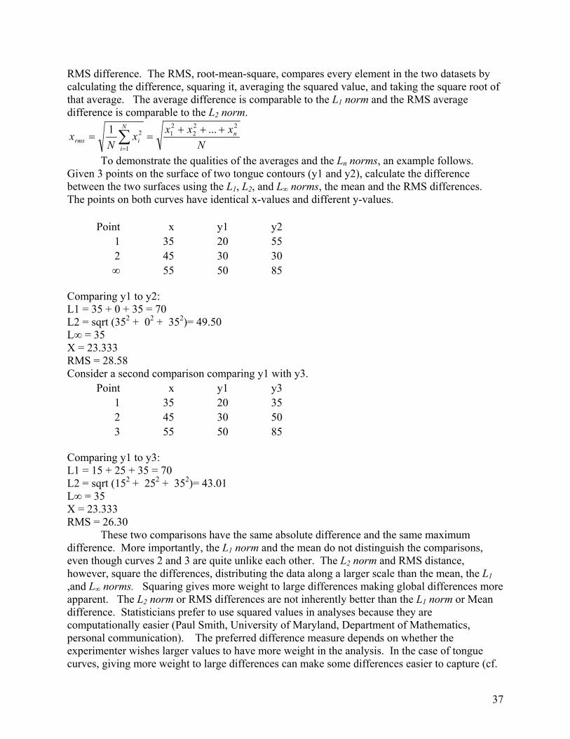
RMS difference. The RMS, root-mean-square, compares every element in the two datasets by calculating the difference, squaring it, averaging the squared value, and taking the square root of that average. The average difference is comparable to the L1 norm and the RMS average difference is comparable to the L2 norm.

Nxxxx

Nx n

N

iirms

222

21

1

2 ...1 +++== ∑

=

To demonstrate the qualities of the averages and the Ln norms, an example follows. Given 3 points on the surface of two tongue contours (y1 and y2), calculate the difference between the two surfaces using the L1, L2, and L∞ norms, the mean and the RMS differences. The points on both curves have identical x-values and different y-values.

Point x y1 y2

1 35 20 552 45 30 30∞ 55 50 85

Comparing y1 to y2: L1 = 35 + 0 + 35 = 70 L2 = sqrt (352 + 02 + 352)= 49.50 L∞ = 35 X = 23.333 RMS = 28.58 Consider a second comparison comparing y1 with y3.

Point x y1 y31 35 20 352 45 30 503 55 50 85

Comparing y1 to y3: L1 = 15 + 25 + 35 = 70 L2 = sqrt (152 + 252 + 352)= 43.01 L∞ = 35 X = 23.333 RMS = 26.30

These two comparisons have the same absolute difference and the same maximum difference. More importantly, the L1 norm and the mean do not distinguish the comparisons, even though curves 2 and 3 are quite unlike each other. The L2 norm and RMS distance, however, square the differences, distributing the data along a larger scale than the mean, the L1 ,and L∞ norms. Squaring gives more weight to large differences making global differences more apparent. The L2 norm or RMS differences are not inherently better than the L1 norm or Mean difference. Statisticians prefer to use squared values in analyses because they are computationally easier (Paul Smith, University of Maryland, Department of Mathematics, personal communication). The preferred difference measure depends on whether the experimenter wishes larger values to have more weight in the analysis. In the case of tongue curves, giving more weight to large differences can make some differences easier to capture (cf.

37

Davidson, 2004). For example, the same mean and L1 norm difference can occur when comparing two curves with a uniform moderate difference versus two curves which differ considerably in one location and minimally at another as in the above example. The L2 norm and RMS difference distinguish these two cases, suggesting an advantage to squaring the data. The mean data have an advantage over the norms in that comparisons using different N’s can be compared using RMS values, but not using Ln norm values, because the average is divided by N; the sum is not. Thus in many cases the RMS difference will be the best of these measures in distinguishing globally between two curves. 7. Using Pellets to Track Tissue Points Pellet tracking has been used in speech research for many years. X-ray Micro beam and various electro-magnetic articulography (EMA) systems track tissue-points on the tongue surface to extract local kinematic information. Point-tracking systems and imaging systems complement each other well. Point tracking systems track single points at high sampling rates, but cannot provide information about the cross-section of the tongue, the pharyngeal shape, or the tongue surface between the points. Imaging systems, including ultrasound, provide that missing information but cannot determine the motion of a specific point on the tongue. Placing pellets on the tongue surface and collecting ultrasound images provides global surface data and local kinematic data, though at slow ultrasound frame rates. Pellets can be tracked accurately in the midsagittal plane because there is little or no lateral motion of the tongue during speech. It is difficult or impossible to use pellet tracking for parasagittal and coronal planes, because the tongue moves in and out of these planes during speech, taking the pellet with it (Shawker et al., 1985). Tracking a pellet using ultrasound presents unusual problems. Because the interface between the tongue surface and air in the mouth is a nearly perfect reflector of ultrasound, it is not possible to reflect a higher amplitude level echo from a point source on the tongue surface. However, it is possible to generate a localized reverberation artifact that projects over the air in the oral cavity. A perfect sphere generates a localized reverberation artifact or what has been described as the ‘Comet Tail’ artifact (Ziskin, Thickman, Goldenberg, Lapayowker, Becker, 1982). This peculiar artifactual pattern was first noted as arising from shotgun pellets within the liver on abdominal ultrasound scanning (Wendell and Athey, 1981). It consists of a dense, homogeneous trail of echo enhancement composed of regularly spaced discrete echo bands that start at and continue beyond the pellet (see figure 7A).

Figure 7A. (a) Pelleton Tongue. (b). Tongue surface with pellet and comet tail.

38

Shawker, et al. (1985) tested multiple objects and shapes that might generate a reverberation artefact. On the tongue surface, both 3 and 5 mm diameter stainless steel ball bearings generated strong reverberation echoes, confirming the hypothesis that the reverberation artefacts are generated by multiple reflections from the anterior and posterior surface of the object. The reverberation artefact is visible until the tongue surface deforms beyond a critical angle, approximately 50° off-axis from the ultrasound beam ray, after which the reverberation artefact begins to disappear,

The pellet must be affixed to the tongue in such a way that the sound enters and reverberates. The adhesive needs to be non-toxic, and equally important, sonolucent, that is, transparent to ultrasound. Adhesives that dry to a brittle consistency are not acceptable, because they refract the sound wave away from the pellet and prevent reverberation. Dental impression materials, the particularly denser ones such as Impregum brand, are successful in affixing the pellet and not impeding the sound wave. Imaging a pellet is more difficult than imaging the tongue surface. It is difficult to find the slice containing the pellet and often there is no reverberation or a weak one, due to any of the problems listed in this section. Instructions for placing a pellet are found in the Acoustical Society of America videotape ‘Measuring Speech Production’ (Stone, 1993). Pellet information complements ultrasound surface measurements. A study comparing imaging and pellet-tracking methodology was done using midsagittal ultrasound and X-ray microbeam data (Stone, 1990). The ultrasound contours were aligned to the X-ray microbeam data by means of common pellet placements (see also section 3a, this paper). Since three points define a plane, visibility of the three pellets ensured that the image sequences were all in the midsagittal plane. The two data sets provided different information about the tongue. The pellets were not always on the point of maximum displacement, seen in the contours. However, the pellet motion revealed local tongue surface stretch consistent with muscle activity and provided insight into the control and kinematics of the movements. Thus, the contour plus the pellets provided greater perspective on tongue behaviour than either provided alone. Pellets can be used to compare gestures between subjects. Stone and Shawker (1986) studied timing relationships between a tongue blade pellet and the hyoid shadow during swallowing and developed a method for normalization of pellet position across subjects. That method is to first affix a pellet onto the protruded tongue at 4.5 cm back from the tip. Standard ultrasound scanning is then used to image the midsagittal tongue. The surface distance from the pellet to the hyoid shadow is measured and added to the 4.5 cm. The first pellet is then remove and, based on the calculated tongue length, replaced with a new one 1/3 of the way back from the tongue tip for each subject. The data collection is performed using the second pellet. This is not a perfect solution since the anterior tongue expands considerably when protruded. In the above study, the 4.5 cm distance was found to be only about 3 cm when the tongue was returned to the mouth. However, the method provides inter-subject normalization for comparing gestures of all sorts. 8. Reconstructing 3D tongue surfaces Three-dimensional (3D) or volumetric ultrasound scanning is offered by several commercial companies. Typically, 3D machines contain a 2D transducer that collects a scan in the ordinary way. The transducer is then moved mechanically to another location (a few degrees away) to collect the next scan. The internal computer reconstructs the echoes and displays a 3D volume plus three 2D planes with multiple slices in each. Multiple repetitions, currently required for 3D reconstruction utilizing other instruments, are not necessary with a 3D transducer, and 3D scanning is as fast as 24Hz. There are

39

two drawbacks to 3D machines, however. First, the data are stored in proprietary format from which only 3D movies or single jpg frames (not a series) can be saved. This makes tongue extraction virtually impossible. Second, there is an enormous amount of data. At 24 fps x 3 dimensions (sagittal, coronal, transverse) x 10+ sections in each dimension, the tongue is represented by 720 frames per second. Thus, even if the images could be stored for analysis, their measurement would be impractical. In addition, the ultrasound technology is the same as that of 2D machines, so image quality is not improved and subjects that image badly in 2D also image badly in 3D. But, in the future, possibly even the near future, these machines could provide very good data. .

8a. Reconstructing 3D static tongue surfaces Using an ordinary (2D) ultrasound transducer to recreate 3D surfaces is, at present, more

convenient for quantitative analysis than 3D machines. A sparse data set of 5-6 coronal slices is adequate to accurately reconstruct 3D surfaces. Stone and Lundberg (1996) and Lundberg and Stone (1999) defined 3D tongue surface shapes for static American English sounds using first a 60 slice, and then sparser, ultrasound data sets. The goal was to determine the optimal number and location of slices needed to reconstruct the tongue surface while minimizing error and maximizing coverage. The sparse sets were compared to the full set. It was determined that 5-6 coronal slices were optimal and provided 80% coverage, a 1.40mm maximum error, and a 0.20mm average error. This result means that only a small number of coronal slices are needed to provide high quality 3D tongue surfaces. See figure 8a.

Although the surface reconstruction is substantially improved by optimising the location of the coronal slices, it is not always possible to do so when collecting data. In that case a set of 5-6 equidistant coronal slices can be used to create a fairly good tongue surface, though with a higher error than in the optimised case. The unoptimised data, which used equidistant slices, had 79% coverage; 2.66mm maximum and 0.37mm average error in the reconstructed surfaces. In addition, collecting additional slices provides better surface detail (cf., Bressman, Thind, Bollig, Uy, Gilbert, Irish, 2005).

Figure 8A. Comparison of 3D reconstructions from full data set (left) and sparse data set (right) for /l/. Differences at probed points shown at bottom. From Lundberg and Stone, 1999.

40

8b. Reconstructing 3D tongue surface motion

Reconstructing 3D surface motion also requires 2D data sets collected at multiple scan locations. The goal is to combine the 2D contour motions into a single 3D tongue surface motion using both temporal and spatial alignment. The spatial position of different scans can be aligned using the location of the transducer. For the temporal alignment, one must take into account that subjects vary in speaking rate and articulation for multiple repetitions. Speaking rate differences are likely when the repetitions are separated in time by other speech materials, as is often the case with multiple ultrasound data sets. A time-warping algorithm is needed to align temporal variations in multiple repetitions. Dynamic programming (DP) algorithms have been used successfully in automatic speech recognition systems to eliminate the effect of large variation in speaking rates and inter and intra-speaker variation (Itakura, 1975; Sakoe and Chiba, 1978; Rabiner and Juang, 1993; Ney and Ortmanns, 1999). The DP algorithm finds the optimal time registration based on the minimum distance between acoustic features in the two repetitions.

Yang and Stone (2002), reconstructed 3D tongue surface motion from ultrasound images using a dynamic programming (DP) algorithm. They temporally aligned 5 coronal and 3 sagittal data sets by applying a DP algorithm to the simultaneously recorded acoustic signals (figure 8B). After time alignment was applied, all the image tokens were aligned temporally and had the same number of frames as the midsagittal sequence. Next the spatial orientation of each coronal contour was determined relative to the midsagittal contour by aligning its transducer position with that of the midsagittal contour. All three sagittal sections were used to check that the spatial positions of the coronal contours were determined properly. The three sagittal contours were also used to reconstruct the tongue tip beyond the anterior-most coronal slice. The anterior points in the sagittal contours were connected with interpolating splines to create a surface. Figure 8C shows the tongue surface for every 6th frame of a sequence of reconstructed surfaces for the speed sample, “It ran a lot.”

I t r B n D l A t

I t r B n D l A t

Figure 8B. DP alignment of two speech waves. From Yang and Stone, 2002.

41

Figure 8C. Sequence of reconstructed frames from a 3D motion image sequence. From Yang and Stone, 2002

9. Conclusions

Ultrasound is a highly functional tool, which once its limits are understood provides an almost unique perspective on tongue motion. Some of ultrasound’s advantages are that it is affordable, requires minimal training and can be used in the laboratory, the clinic, or the field. Ultrasound reveals substantial information about tongue deformations because it can record multiple planes, each in real-time. In the sagittal plane, most of the tongue’s length, including the pharynx is visible. Multiple coronal and oblique planes can also be measured to study local motion or reconstruct 3D behaviours. Ultrasound also has limitations, though many are surmountable. Some correctable limitations include extracting the tongue surface from a noisy image, the need for holders and devices to convert this clinical technique into a research instrument, the lack of a reference structure in the image and the lack of tissue point information. Ultrasound has other limitations that must be accepted, such as the inability to image the tip and lateral margins of the tongue. Ultrasound can be used in combination with other instruments to increase the comprehensiveness of tongue analysis. One of the challenges and advantages of ultrasound is the high-dimensionality of its data. High-dimensionality is a challenge because numerical quantities must be used to reduce the dimensionality in order to perform statistical comparisons, and adequately interpret results. High-dimensionality is an advantage because the complex tongue surface deformations are well represented by the data. Acknowledgements: The author would like to thank Lisa Davidson, Melissa Epstein and Marianne Pouplier for their helpful comments on the manuscript. The research was supported in part by NIH grant R01-DC01758 from the NIDCD.

42

References Bressman, T., Thind, P., Bollig, C.M., Uy, C., Gilbert, R.W., & Irish, J.C. (2005) Quantitative three-dimensional ultrasound analysis of tongue protrusion and grooving: Data from twelve normal speakers and a partial glossectomee. International Journal of Clinical Linguistics and Phonetics Chi-Fishman, G. (2005). Quantitative lingual, pharyngeal and laryngeal ultrasonography in swallowing research: A technical review. International Journal of Clinical Linguistics and Phonetics Curie J., & Curie P. (1880). Sur l’électricité polaire dans les cristaux hémièdres à faces inclinées. CR Séances Acad Sci, 91, 383-386. Davidson, L. (2004). Assessing tongue shape similarity: Comparing norms, area, and average distance. Talk presented at Ultrafest II, University of British Columbia, Vancouver, Canada. April 22-23, 2004. Davis, E.P. (1999). Measurement and kinematic modeling of the human tongue. Ph.D. Dissertation, Johns Hopkins University, Department of Mechanical Engineering. Dussik K. (1942). Über die Möglichkeit hochfrequente mechanische Schwingungen als diagnostisches Hilfsmittel zu verwenden. Z Gezamte Neurol Psych, 174, 153-168. Epstein, M. (2005). Ultrasound and the IRB. International Journal of Clinical Linguistics and Phonetics Gick, B., Bird S., & Wilson, I. (2005). Techniques for field application of lingual ultrasound imaging. International Journal of Clinical Linguistics and Phonetics Harshman, R., Ladefoged, P., & Goldstein, L. (1977). Factor analysis of tongue shapes. Journal of the Acoustical Society of America 62, 693-707. Hedrick, W.R., Hykes, D.L., & Starchman, D.E. (1995) Ultrasound Physics and Instrumentation, third Edition: Mosby Inc.: St Louis Mo Hoole, P. (1999). On the lingual organization of the German vowel system. Journal of the Acoustical Society of America. 106(2), 1020-1032. Iskarous, K. (2005). Detecting the edge of the tongue: A tutorial. International Journal of Clinical Linguistics and Phonetics Itakura,F. (1975). Minimum prediction residual principle applied to speech recognition. IEEE Trans. Acoust. Speech signal process. ASSP, 23, 67-72. Jackson, M. (1988) Analysis of tongue positions: Language-specific and cross-linguistic models. Journal of the Acoustical Society of America, 84, 124-143. Li, M., Kambhamettu, C. & Stone, M.( 2005a). Automatic Contour Tracking in Ultrasound Images. International Journal of Clinical Linguistics and Phonetics Li, M., Kambhamettu, C., & Stone, M (2005b) International Journal of Clinical Linguistics and Phonetics Ludwig G.D., & Struthers F.W. (1949). Considerations underlying the use of ultrasound to detect gallstones and foreign bodies in tissue. Project MN 004-001 Naval Medical Research Institute, 4: 1. Lundberg, A., & Stone, M. (1999). Three-dimensional Tongue Surface Reconstruction: Practical Considerations for Ultrasound Data. Journal of the Acoustical Society of America, 106, 2858-2867. Lundstrom, F., & Lundstrom, A. (1992) Natural head position as a basis for cephalometric analysis. American Journal of Orthodontics and Dentofacial Orthopedics, 101, 244-247.

43

Maeda, S. (1990). Compensatory articulation during speech: evidence from the analysis and synthesis of vocal-tract shapes using an articulatory model. Speech production and speech modeling. Dordrecht: Kluwer Academic Publication (Ed. Hardcastle, W. and Marchal, A.), 131-150. Miller, J. L., & Watkin, K. L., (1997). Lateral pharyngeal wall motion during swallowing using real time ultrasound. Dysphagia, 12, 125-132. Moody, J. (1998), Visualizing Speech with a Recurrent Neural Network Trained on Human Acoustic-Articulatory Data, Ph.D. Dissertation, Department of Cognitive Science, UC San Diego, page 43. Moorrees, C. (1994), Natural head position: a revival. American Journal of Orthodontic and Dentofacial Orthopedics, 105, 512-514. Morrish, K., Stone, M., Shawker , T., & Sonies, B.C. (1985). Distinguishability of tongue shape during vowel production. Journal of Phonetics, 13(2), 189-204. Morrish, K., Stone, M., Sonies, B., Kurtz, D., & Shawker, T. (1984). Characterization of tongue shape, Ultrasound Imaging, 6(1), 37-47. Ney, H., & Ortmanns, S. (1999). Dynamic programming search for continuous speech recognition. IEEE Signal Processing, 16(5), 64-83 Ostry, D., Keller, E., & Parush, A. (1983). Similarities in the Control of the Speech Articulators and the limbs: Kinematics of Tongue Dorsum Movement in Speech. Journal of Experimental Psychology: Human Perception and Performance, 9, 622-636. Parthasarathy, V., Prince, J.L., & Stone, M. (2005). Spatiotemporal Visualization of the Tongue Surface using Ultrasound and Kriging (SURFACES). International Journal of Clinical Linguistics and Phonetics Peng, C., Jost-Brinkmann, P., & Miethke, R. (1996). The Cushion Scanning Technique: A method of dynamic tongue sonography and its comparison with the transducer skin coupling scanning technique during swallowing. Academic Radiology, 3, 239-244. Peng, C., Jost-Brinkmann, Yoshida, N., Cou, H., & Lin, C. (2004) Comparison of tongue functions between mature and tongue thrust swallowing – an ultrasund investigation. American Journal of Orthodontics and Dentofacial Orthopedics, 125, 562-570. Rabiner, L. & Juang, B-H. (1993). Fundamentals of speech recognition. PTR Prentice-Hall Inc., New Jersey. Sakoe, H. & Chiba, S. (1978). Dynamic programming algorithm optimization for spoken word recognition. IEEE Trans. Acoust. Speech Signal Process, 26, 43-49. Shawker T., Sonies B.C., & Stone, M. (1984). Soft Tissue anatomy of the tongue and floor of the mouth: An ultrasound demonstration. Brain and Language, 21, 335-350. Shawker, T., Stone, M., & Sonies, B.C. (1985). “Tongue pellet tracking by ultrasound: Development of a reverberation pellet,” Journal of Phonetics, 13, 135-146. Slud, E., Stone, M., Smith, P. & Goldstein, M. (2002). Principal Components Representation of the Two-Dimensional Coronal Tongue Surface. Phonetica, 2002, 59, 108-133. Sonies B.C., Shawker T.H., Hall, T.E., Gerber L.H., Leighton S.B. (1981). Ultrasonic visualization of tongue motion during speech. Journal of the Acoustical Society of America, 70 (3), 683-686 Stone, M. (1990). A three-dimensional model of tongue movement based on ultrasound and x-ray microbeam data. Journal of the Acoustical Society of America, 87, 2207-2217.

44

Stone, M. & Davis, E. (1995). A head and transducer support (HATS) system for use in ultrasound imaging of the tongue during speech. Journal of the Acoustical Society of America, 98, 3107-3112. Stone, M., Goldstein, M., & Zhang, Y. (1997). Principal component analysis of cross-sectional tongue shapes in vowels. Speech Communication, 22, 173-184. Stone, M. & Lele, S. (1992). Representing the tongue surface with curve fits. Proceedings of the International Conference in Spoken Language Processing, Banff, CA, 2 (Oct.), 875-878. Stone, M. & Lundberg, A. (1996). Three-dimensional tongue surface shapes of English consonants and vowels. Journal of the Acoustical Society of America, 99, 3728-3737. Stone, M., Morrish, K., Sonies, B., & Shawker, T. (1987). Tongue curvature: A model of shape during vowel production. Folia Phoniatrica, 39, 302-315. Stone, M., Parthasarathy, V., Pabla, T., Sutton, M., & Crouse, U (2002). Exploring the effects of gravity on tongue motion using ultrasound image sequences. Journal of the Acoustical Society of America, 111(5), Pt. 2, 2476A. Stone, M. & Shawker, T. (1986). An ultrasound examination of tongue movement during swallowing. Dysphagia, l, 78-83.Stone, M., Shawker, T., Talbot, T., & Rich, A. (1988). Cross-sectional tongue shape during the production of vowels. Journal of the Acoustical Society America, 83 (4), 1586-1596. Stone, M., Sonies, B., Shawker, T., Weiss, G., & Nadel, L. (1983). Analysis of real-time ultrasound images of tongue configuration using a grid-digitizing system. Journal of Phonetics, 11, 207-218. Stone, M., Sutton, M. Parthasarathy, V., Prince, J., Li, M., & Kambhamettu, C (2002). Effects of upright and supine orientation on tongue position during silence. Joint meeting of the Acoustical Society of America, Iberoamerican Congress of Acoustics and Mexican Congress on Acoustics. Cancun, Mexico. December 2-6, 2002. Stone, M., & Vatikiotis-Bateson, E. (1995). Trade-offs in tongue, jaw and palate contributions to speech production. Journal of Phonetics, 23, 81-100. Sze, Cheng-Feng, (2000), Reconstructing 3D tongue motion from 2D ultrasound images and speech signals. PhD. Dissertation, Dept. of Electrical and Computer Engineering, University of Maryland, College Park, p. 54-76. Viazis, A.M., (1991), A cephalometric analysis based on natural head position. Journal of Clinical Orhodontics, 25, 172-181. Wendell, B.A.,& Athey, P.A. (1981). Ultrasonic appearance of metallic foreign bodies in parenchymal organs. Journal of Clinical Ultrasound, 9(3),133-5. Whalen, D. H., Iskarous, K., Tiede, M. T., Ostry, D., Lehnert-LeHoullier, H., & Hailey, D. (in press). HOCUS, the Haskins Optically-Corrected Ultrasound System. Journal of Speech, Language, and Hearing Research. Yang C., & Stone, M. (2002). Dynamic Programming Method for Temporal Registration of Three Dimensional Tongue Surface Motion from Multiple Utterances. Speech Communication 38 (1-2):199-207. Ziskin, M.C, Thickman, D.I., Goldenberg N.J., Lapayowker M.S. & Becker, J.M. (1982). The comet tail artifact. Journal of Ultrasound in Medicine. 1 (1): 1-7.

45

46