A Global Database of Foreign Affiliate Activity

Tani Fukui1

Csilla Lakatos2

Abstract

This paper produces a new dataset to further the literature on the behavior of multinational firms. The Eurostat database, with a large number of sector-level, bilateral observations on foreign affiliate sales, provides a basis from which to extrapolate the relationships between various host and source country factors and the foreign affiliate activity produced by them. This paper exploits the detailed level of the data by introducing sector-specific variables which in turn permit out of sample predictions. Further, the large number of excess zeros in the Eurostat dataset presents added complexity and is addressed using techniques borrowed from the trade literature, which also experiences a “zeros” problem. The datasets produced in this paper also serves as an input into the FDI-GTAP model of Lakatos and Fukui (2012). This model integrates the datasets produced in this paper into a model that permits the analysis of the behavior of foreign affiliates within the context of a general equilibrium model. The dataset is combined with other data on foreign affiliate sales and together with an optimization procedure produces a new dataset based on all of existing data sources.

I. Introduction

The examination of foreign affiliate data is a relatively new branch of the literature, owing primarily to the paucity of data in this area of research. Foreign direct investment (FDI) statistics are collected by numerous countries, but these do not provide a complete picture of the activities of multinational enterprises. In particular, FDI examines only the international transfer of funds rather than their operations. Without data on operations of multinationals, it is difficult to assess the effect of policy changes on foreign affiliate activity. As foreign affiliate activity grows in importance, this lack of data is slowly being addressed, and research is able to move forward. In particular, the establishment of the Eurostat database provides a much needed boost for in this area of research. Eurostat provides a large amount of data on foreign affiliate activity, rather than data only on investment stocks or flows. This paper uses the Eurostat dataset to estimate the behavior of foreign affiliate sales as a basis. It implements an econometric model consistent with the branch of the literature that originated in Markusen, et al (1996)

1

1 Corresponding author. Tani Fukui (tani.fukui@usitc.gov) is an economist at the U.S. International Trade Commission from the Office of Economics. These views are strictly those of the author and do not represent the opinions of the U.S. International Trade Commission or of any of its Commissioners.

2 Csilla Lakatos is a Post-Doctoral Research Associate at the Department of Agricultural Economics at Purdue University and Visiting Fellow at the U.S. International Trade Commission.

and Markusen (1997) and that includes Bergstrand and Egger (2007) and Carr, Markusen, and Masksus (2001).

Blonigen (2005) provides a comprehensive review of the recent literature on FDI determinants. He concludes that the broad-based relationships between FDI and policies have been difficult to come by.3 More importantly, he assesses that as FDI research progresses (it is still a relatively new area of research), it will continue to be thwarted in its search for overarching relationships, primarily because the reasons for which firms invest abroad are many and varied.

The economic literature on the drivers of FDI identifies two main types of investment rationales: market access (selling to consumers in the host market) and efficiency seeking (searching for low cost production sources). In addition, the proliferation of global supply chains has led to variations on each of these themes, so that goods (and to a lesser extent services) pass through multiple countries with final consumption sometimes taking place in one of the production countries, so that both efficiency seeking and market access motivate the foreign investment.

This heterogeneity can best be addressed by examining the matter at a more detailed level—honing in on particular sectors or countries, in which the investment rationale may be more uniform. As a result, the literature has increasingly gone the way of firm-level analysis, which permits the researcher to control more tightly by type of investment rationale. Despite this trend, we follow the literature in examining macro-level FDI statistics. However, in many cases, such as for the project we have taken on, it is necessary to make some assessment of overall macroeconomic behavior, although it may simply be a rough approximation of true firm behavior. Firm-specific effects cannot hope to provide approximations of macro-level activity, as well as a matter of practicality in attempting to estimate these effects for a large number of countries.

A problem presented by this dataset is the existence of a large number of missing values. This is a problem that has not been extensively addressed in the FDI literature. On the other hand, it has been addressed in the trade literature, which also has such problems. We integrate some approaches of that literature in our estimation strategy, in particular, the Pseudo Poisson Maximum Likelihood proposed by Santos, Silva, and Tenreyro (2005) and the zero inflated models discussed in De Benedictis and Taglioni (2011). Finally, there has been very little use of sector specific data in foreign affiliate data research, largely because it is not usually available. We take advantage of this extra dimension in the model to attempt to estimate sector-specific differences in foreign affiliate activity using sector specific data.

2

3 The study examines both investment stocks and flows as well as operations of multinationals.

In addition to the zeros problem, there is also a large number of missing values in the database that prevents the immediate use of these data in the FDI-GTAP model. This is due both to confidentiality or missing values (so that source-host-sector points are not available in many cases), and also to the constrained set of countries in the database. The database documents data to and from European countries only. In order to apply the database to the full FDI-GTAP model, it is necessary to extrapolate to all regions used in the GTAP model. The coefficients generated from the econometric analysis in this paper will be used as a starting point for the extrapolation.

This paper is one of two papers produced in tandem to provide a rich modeling tool for policy analysis. Our goal is to construct a set of tools to model the behavior of foreign affiliates. In order to properly model this, we need two elements: a set of databases and a model. We first construct a set of three databases that enable the breakdown of “domestic” elements of the economy into foreign and domestic elements – in particular, foreign capital stocks, value added, and foreign affiliate sales.

In order to properly model the behavior of foreign affiliates, Then we feed these databases into a modified version of the GTAP model (version 8). This is a data-driven general equilibrium model that models the global economy at a detailed regional and sectoral level, using 129 countries and regions and 57 sectors. The main focus of this model is the modeling of international trade and in particular modeling the effects of trade policies on the economic welfare on countries. We modify this model to explicitly take into account the existence of foreign owned capital and foreign affiliate activity. The construction of the databases is detailed in this chapter; the construction of the model and its policy implications are in Lakatos and Fukui (2012).

To our knowledge, there has been only one prior attempt, in Hanslow (2000), to construct a large scale, bilateral by sector, fully consistent database of foreign affiliate statistics. The purpose of that database was, as with ours, to use it within a version of the GTAP model modified to include FDI. There are a few key differences between their estimation attempt and ours is as follows. Hanslow (2000) used ratios of foreign affiliates data—total assets to FDI capital and sales to asset ratios—by sector, extracted from U.S. BEA data , and applied those ratios to FDI stocks reported by CEPII. Similar ratios were used for value added. In our method, we broaden the set of underlying countries to include all European countries reported in the Eurostat database (the full list of countries is below) rather than relying solely on U.S. data. In addition we estimate the effects using a fully specified econometric model which does indeed display significant differences across both host and source countries, as well as across sectors. The use of econometrics within this context, therefore, is new. In addition, due to improvements in data collection by Eurostat, it has become possible to examine the cost structure of foreign affiliates using value added and

3

employment costs. Therefore, rather than relying on calculations of value added based on pro rata allocations from sales, we are able to directly estimate the labor and capital shares of value added.

In the second section we provide some background literature on prior estimation of foreign affiliate activity. The third section focuses on the estimation of foreign affiliate sales, including data source and estimation model, with the fourth section discussing the results. A fifth section presents some additional estimates that will be necessary to construct the final database. A sixth section describes the quadratic optimization procedure and presents elements of the final database. The seventh section details the estimation of value added. A final section concludes.

II. Background

There is currently no global database of foreign affiliate sales. The closest such source available to us is the Eurostat database which has detailed sectoral level foreign affiliate sales by source country for many European countries. In order to construct the required database, we first conduct an econometric analysis of the existing data to produce a set of coefficients that provide information about the relationship between various independent variables and foreign affiliate sales. These coefficients are then used to extrapolate to the full set of countries and sectors needed by the GTAP model.4 Finally, the extrapolated dataset is merged with the known data: these data include the original Eurostat dataset as well as data from the OECD, the U.S. BEA, and UNCTAD. Contradictory information among these data sources is resolved using an optimization procedure explained in detail in section VI.

There is a small but growing literature that has in recent years attempted to produce a well-formed model for the use of gravity-like models for FDI and foreign affiliate activity in the way that Anderson and van Wincoop (2003) have done for trade flows. Generally, the literature on FDI follows closely that of trade. The gravity model, frequently employed to explain trade flows, has also been employed to explain FDI. As with trade, the rationale for the gravity model began as a practical matter: the model “worked” in that it had a high degree of explanatory power, but the theoretical foundations were shaky or non-existent. In recent years, however, progress has been made in providing theoretical underpinnings to the model. These theories have naturally also produced modifications that are FDI-specific and warrant close attention.

The set of models described in Markusen (2002) is one of few strands of literature to explicitly examine foreign affiliate sales rather than FDI. Kleinert and Toubal (2010) also present a model on foreign

4

4 Certain sectors are aggregated from the original GTAP model, including particularly the agriculture sectors.

affiliate sales, lending further support to a gravity-type model. The original paper by Markusen discusses a 2 factor, 2 country, 2 good (2 x 2 x 2) knowledge capital model, whose main contribution is to delineate the difference between horizontal multinationals (those firms that establish subsidiaries abroad to sell in those markets) and vertical multinationals (those firms that establish subsidiaries abroad to reduce production costs).

In Carr, Markusen, and Maskus (2001), a horizontal and a vertical model are nested within the knowledge capital model in order to test whether one or the other is supported by the data. The results of these tests reject the vertical model, and cannot reject the horizontal. That is, at the aggregate level, the data demonstrate more horizontal than vertical characteristics. The data used are U.S.-associated values only (foreign affiliate sales), aggregated to the bilateral level. They do not have sector level data. Rather than an OLS model, they use WLS as well as a Tobit model. The main concern is heteroskedasticity because countries differ dramatically in size. The weights come from OLS residuals of the sum of GDP values. The Tobit regressions are conducted in order to address prevalence of zero values in the data.

Bergstrand and Egger (2007) (henceforth BE) uses an updated version of the model that advances this literature in a parallel way to the trade literature. This paper presents a 3 factor, 3 country, 2 good knowledge capital model that builds on Carr, Markusen and Maskus (2001) (henceforth CMM). The model in BE adds a third country: this permits the examination of third country effects on bilateral trade flows. That is, it attempts to examine whether the gravity relationships found in the trade literature also hold for foreign affiliate sales (and also for FDI). In particular, they attempt to examine essentially whether an Anderson and van Wincoop type effect is present, i.e. the multilateral resistance term. As noted by BE, most models in the FDI literature examine a two country model rather than a multi-country model which does not permit multilateral resistance terms.

In addition, they add a third factor (capital) that together with the third country produces complementarity between country size and the various trade variables (trade, foreign affiliate sales, and foreign direct investment). In the original 2x2x2 model of CMM, the national and multinational firms were mutually exclusive so that the existence of multinationals would mean that all single-country firms would cease to exist; this is counter to what is observed in the data.

Yeaple (2003) is a rare example in the literature of a paper that uses sector-specific data to distinguish FDI behavior. He uses U.S. BEA foreign affiliate sales data at the bilateral and sectoral level. Yeaple uses the following sector specific information: transport costs (industry and host country specific), a measure of

5

scale economies (industry specific), and a set of variables that reflect unit costs (industry and host country specific).5

III. Data and Econometric Specification

The model we use is based on a modified version of BE and CMM. The BE paper and CMM have largely similar econometric specifications. We modify them in the following ways. First, based on the results presented in the BE paper, the FAS behaves similarly to FDI and so we replace the FDI with FAS. Second, we account for the sector specific nature of our data by replacing the GDP of host countries with the domestic production by sector. We follow Anderson and van Wincoop (2004) in replacing GDP of the host country with domestic production rather than adding this to the regression.

(1)

The subscript i refers to sectors, r refers to host; s refers to source, and t refers to time. The model

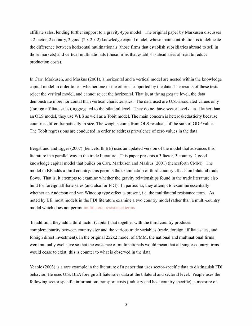
includes a full set of time dummies, . All independent variables are listed in table 1, along with the data source used and summary statistics. GDP is the GDP of the source country. There is considerable variation in the GDP variables, despite the fact that the countries are predominantly European countries, reflecting that both large and small countries are included in the sample. These data are from World Bank World Development Indicators.

6

5 Anderson and van Wincoop (2004) also presents a sector level model, although it is to explain trade flows rather than foreign affiliate activity.

Table 1. Independent Variable

Years available Source

Dimension Units* Mean Median MinimumMaximum

Standard Deviation

Foreign affiliate sales

2003-2007

Eurostat (FATS)

sector, source, host, date

$ million 140 0 0 54,100 1,090

GDP, source through 2009

World Bank source, date

$ billion 830 233 5 14,000 1,920

GDP, host through 2009

World Bank source, date

$ billion 526 179 10 3,320 771

Domestic production, host

2007 Eurostat host, sector

$ million 14,700 1,780 0.4 584,000 49,200

GDP RoW through 2009

World Banksource, host, date

$ billion 44,800 45,000 24,500 55,700 6,370

Distance n.a. CEPII source, host

km 3,314 1,727 161 19,539 4,215

Common language (ethno)

n.a. CEPII source, host

0 or 1 (1 = common language)

0.03 0 0 1.00 0.16

Economic Freedom: Trade

1995-2008

Economic Freedom Network

host, date scale of 1 to 10 (1 = most restricted)

8.5 8.5 6.8 9.8 0.6

Economic Freedom: Investment

1995-2008

Economic Freedom Network

host, date scale of 1 to 10 (1 = most restricted)

6.7 6.7 4.3 8.6 0.9

FDI restrictiveness

2010 OECD (2010)

sector, host

Scale of 0 to 1 (1 = most restricted)

0.02 0 0 1.0 0.1

Skill difference 1989-2008

ILO source, host, date

skill/unskilled ratio of source less host

-0.006 0.001 -0.39 0.29 0.10

GDP per capita, source

through 2009

World Bank source, date

$ 25,013 23,682 1,731 82,294 16,160

GDP per capita, host

through 2009

World Bank host, date $ 22,230 18,424 2,555 56,894 14,386

* Units are as reported here for ease of notation; for the regressions we use whole dollar values (rather than millions, etc.) for all values. Note: Summary statistics include only those observations that were ultimately included in regressions. There were a total of 41,083 observations with a complete set of independent variables, including those for which foreign affiliate sales was zero.

7

GDP RoW is the GDP of the rest of the world, i.e. GDP of the world less GDP of both source and host countries’ capital cities. The variation of this variable is quite small, as the size of countries is generally dwarfed by the size of global GDP. These data are also from WDI Online.

Rather than GDP of host, we use domestic production of individual sectors, Prod. This includes both domestically- and foreign-owned firms. This also has a large standard deviation, reflecting both varying sizes of countries and of sectors. These data are also from Eurostat and correspond to the same sectors provided in the foreign affiliate sales database.

Other variables used in gravity type models are distance, Dist, the distance between source and host, and Comlang, a binary variable that takes the value of 1 if source and host share at least one language.

Comlang is predominantly 0, taking on the value 1 in only a handful of cases. Both this and the distance variables were obtained from CEPII.Trade openness is a measure of aggregate trade restrictiveness set up by the host country. This index is obtained from the Fraser Institute’s Economic Freedom of the World report, which uses primarily quantifiable measures on a range of topics to measure a country’s economic freedom. The trade index, “Freedom to Trade Internationally”, takes into account total revenues from tariffs, mean tariffs and the variance of tariffs across tariff lines.

It is clear from the summary statistics that the openness observations are dominated by European countries that have extremely low trade barriers. As a result, the minimum level of trade openness reported is quite high (6.8 out of a possible 10), and the average, at 8.5, represents something substantially close to free trade. There is little variation in this variable.

Investment openness is a measure of investment restrictiveness of the host country. This is also taken from the Fraser Institute’s Economic Freedom of the World report. The investment measure measures international capital market controls, including restrictions on foreign ownership as well as the number of capital controls put in place by a country. There is slightly more variation of this variable than in the trade openness variable, but it is similarly affected by the sample of countries in the Eurostat database.

The FDI restrictiveness index was obtained for G20 countries using Koyama and Golub (2006). This is a sector specific restrictiveness index, which takes into account foreign ownership and other national treatment aspects of investment. The index is similar to the EFW investment index but the EFW index offers a time series while the Koyama and Golub index offers sectoral detail.

8

The variable ∆SK is the skill difference between two countries: the ratio of skilled to unskilled workers in the source country less the same ratio for the host country:

where SK is skilled labor, defined as subclassification 1, 2, or 3 (legislators, senior officials and managers; professionals; and technicians and associate professionals) by the ILO.6 This is a negative number at the mean, so that the average source country in our sample has less skilled workers (relative to its stock of unskilled workers) than the average host country. This makes sense because all host countries are developed countries in the EU while source countries include both developed and developing countries. Countries that are in the source list but not in the host country list include China, Russia and Turkey. There is a great deal of variation among countries in this variable.

The rationale is that countries have a comparative advantage in certain sectors and develop strong multinational firms in those sectors with transferable skills that in turn invest abroad. Domestic production shares are also included as host country variables to capture the effect of a country that has a pronounced comparative advantage that is not transferable. This is most explicit in natural resources, but may also be a factor in manufacturing industries, where countries specialize in specific manufacturing sectors.

Foreign Affiliate Sales Data

The primary data source that we use in our analysis is Eurostat’s data on Foreign Affiliates.7 This is our set of dependent variables. The dataset contains 41 source and 22 host countries (see appendix tables A-1 and A-2). The host countries are the reporting countries, and are all European; most, but not all, source countries are European. The database provides “three dimensional” data: foreign affiliate sales by source country, host country, and sector. A total of 117 sectors and subsectors are covered in the original database. Only a relatively small subset of 21 sectors was selected—this is both because of lack of the corresponding sectoral data of an independent variables, domestic production, and to more closely match the targeted GTAP sectors. The database spans the years 2003 to 2007.

9

6 ILO.org’s LABORSTA database. Labor force survey data were used for all countries: http://laborsta.ilo.org/

7 Variable fats_g1a_03 under the category “Foreign control of enterprises - breakdown by economic activity and a selection of controlling countries”. Accessed May 17, 2011. Data are originally in Euros and presented throughout this paper in US dollars. These data are from the inward FATS data collection, so that host countries are the reporting countries.

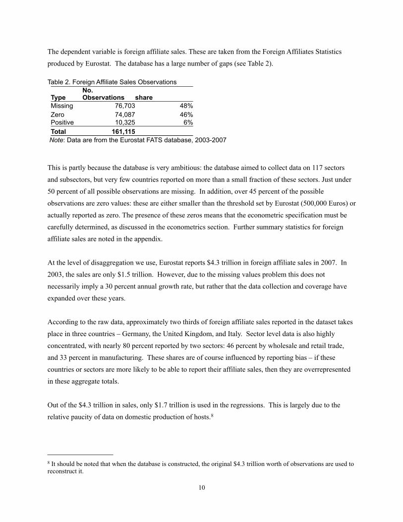
The dependent variable is foreign affiliate sales. These are taken from the Foreign Affiliates Statistics produced by Eurostat. The database has a large number of gaps (see Table 2).

Table 2. Foreign Affiliate Sales Observations

TypeNo. Observations share

Missing 76,703 48%Zero 74,087 46%Positive 10,325 6%Total 161,115

Note: Data are from the Eurostat FATS database, 2003-2007

This is partly because the database is very ambitious: the database aimed to collect data on 117 sectors and subsectors, but very few countries reported on more than a small fraction of these sectors. Just under 50 percent of all possible observations are missing. In addition, over 45 percent of the possible observations are zero values: these are either smaller than the threshold set by Eurostat (500,000 Euros) or actually reported as zero. The presence of these zeros means that the econometric specification must be carefully determined, as discussed in the econometrics section. Further summary statistics for foreign affiliate sales are noted in the appendix.

At the level of disaggregation we use, Eurostat reports $4.3 trillion in foreign affiliate sales in 2007. In 2003, the sales are only $1.5 trillion. However, due to the missing values problem this does not necessarily imply a 30 percent annual growth rate, but rather that the data collection and coverage have expanded over these years.

According to the raw data, approximately two thirds of foreign affiliate sales reported in the dataset takes place in three countries – Germany, the United Kingdom, and Italy. Sector level data is also highly concentrated, with nearly 80 percent reported by two sectors: 46 percent by wholesale and retail trade, and 33 percent in manufacturing. These shares are of course influenced by reporting bias – if these countries or sectors are more likely to be able to report their affiliate sales, then they are overrepresented in these aggregate totals.

Out of the $4.3 trillion in sales, only $1.7 trillion is used in the regressions. This is largely due to the relative paucity of data on domestic production of hosts.8

10

8 It should be noted that when the database is constructed, the original $4.3 trillion worth of observations are used to reconstruct it.

Estimation Strategy

The large number of zero cells in the dataset calls into question the conventional strategy used in the FDI literature. Much of the literature on FDI uses OLS to estimate the relationship between FDI and the dependent variables. The log transformation commonly used in OLS does not permit an explanation for zeros. More problematically, OLS does not model the decision to enter (or not enter) a market as a separate process but rather simply models zeros as part of a linear function.

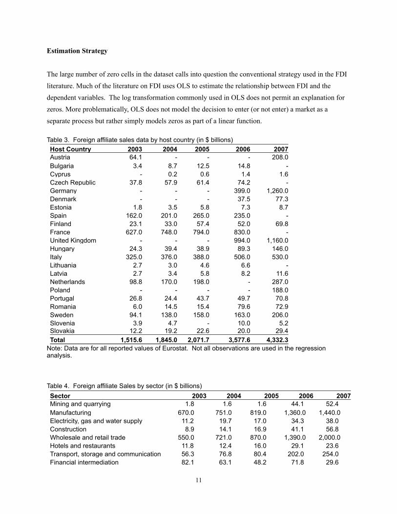
Table 3. Foreign affiliate sales data by host country (in $ billions)Host Country 2003 2004 2005 2006 2007Austria 64.1 - - - 208.0 Bulgaria 3.4 8.7 12.5 14.8 - Cyprus - 0.2 0.6 1.4 1.6 Czech Republic 37.8 57.9 61.4 74.2 - Germany - - - 399.0 1,260.0 Denmark - - - 37.5 77.3 Estonia 1.8 3.5 5.8 7.3 8.7 Spain 162.0 201.0 265.0 235.0 - Finland 23.1 33.0 57.4 52.0 69.8 France 627.0 748.0 794.0 830.0 - United Kingdom - - - 994.0 1,160.0 Hungary 24.3 39.4 38.9 89.3 146.0 Italy 325.0 376.0 388.0 506.0 530.0 Lithuania 2.7 3.0 4.6 6.6 - Latvia 2.7 3.4 5.8 8.2 11.6 Netherlands 98.8 170.0 198.0 - 287.0 Poland - - - - 188.0 Portugal 26.8 24.4 43.7 49.7 70.8 Romania 6.0 14.5 15.4 79.6 72.9 Sweden 94.1 138.0 158.0 163.0 206.0 Slovenia 3.9 4.7 - 10.0 5.2 Slovakia 12.2 19.2 22.6 20.0 29.4 Total 1,515.6 1,845.0 2,071.7 3,577.6 4,332.3

Note: Data are for all reported values of Eurostat. Not all observations are used in the regression analysis.

Table 4. Foreign affiliate Sales by sector (in $ billions)Sector 2003 2004 2005 2006 2007Mining and quarrying 1.8 1.6 1.6 44.1 52.4 Manufacturing 670.0 751.0 819.0 1,360.0 1,440.0 Electricity, gas and water supply 11.2 19.7 17.0 34.3 38.0 Construction 8.9 14.1 16.9 41.1 56.8 Wholesale and retail trade 550.0 721.0 870.0 1,390.0 2,000.0 Hotels and restaurants 11.8 12.4 16.0 29.1 23.6 Transport, storage and communication 56.3 76.8 80.4 202.0 254.0 Financial intermediation 82.1 63.1 48.2 71.8 29.6

11

Real estate 124.0 185.0 204.0 404.0 430.0 Total 1,516.1 1,844.7 2,073.1 3,576.4 4,324.4

Note: Data are for all reported values of Eurostat. Not all observations are used in the regression analysis.

The trade literature has examined this problem extensively, as trade data also tends to have a large number of zeros. In our estimation procedure, we implement both OLS and several other methods borrowed from the trade literature, modified to include FDI-relevant variables.

However two possible problems have been pointed out by other researchers. Santos Silva and Tenreyro (2005) propose the use of Poisson Pseudo Maximum Likelihood (PPML). The original purpose of this method was to address the pervasive heteroskedasticity in the gravity equations rather than specifically addressing excess zeros. However, the Poisson distribution does permit zeros to occur, allowing an explanation of the prevalence of zeros. They demonstrate that Poisson performs well under certain heterogeneity conditions.

Some arguments have been raised against the use of the PPML model. First, that it under-predicts the number of zeros; second that there is over-dispersion as PPML requires that mean and variance be roughly equal. These arguments have been put forth in Martin and Pham (2008) and De Benedictis and Taglioni (2011) . The latter has proposed other methods such as the zero inflated models ZIP (zero inflated Poisson) and ZINB (zero inflated negative binomial). Zero-inflated models are models that combine a logit model with a Poisson type model. As a result, there are two possible ways in which these models can generate a zero: first, under the logit portion of the model, which predicts a binary go/no go decision; and second under the main part of the model which, conditional on a “go” decision of the logit model, predicts the value of that decision. ZIP and ZINB behave similarly with the one difference that the ZINB does not force equality between mean and variance. Both sufficiently high fixed and variable costs may generate zero foreign affiliate sales. It should be noted that the mere existence of overdispersion does not require the selection of ZINB over ZIP. ZIP, by virtue of its two processes, may yield an over-dispersed set of predicted values.

An added complication is that reported zeros in the Eurostat database do not all mean zero. They may be either small positive values (less than 500,000 Euros) or true zeros. There is no way of distinguishing the two cases given the currently available data.

IV. Results

12

The results of the main econometric estimation are presented in table 5. Each of the four results in the table use the same set of independent variables. The first column in table 5 uses OLS, the second uses PPML, the third uses ZIP and the fourth column use ZINB.

According to BE, the expected sign of GDP source is positive.9 In our estimation, this is not the case for any of the estimation results (1)-(4) in table 5. As a result GDP of the source country appears to be negatively (and significantly in every case except for PPML) correlated with foreign affiliate sales. However, the GDP of the rest of the world (GDP RoW) has a large negative coefficient. Because this variable is inversely related to the GDP of the source country, the net effect of these two coefficients is such that GDP of the source country is positively correlated with foreign affiliate sales. That is, the positive effect of GDP source and host are captured in the highly negative coefficient of GDP RoW.

The expected sign of GDP RoW is negative. As noted above, this is indeed the case. Note that this coefficient is particularly large (and negative) for PPML. That is, the joint size of host and source country are a particularly strong driver of activity according to the PPML estimate but somewhat less so for the other estimates.

Domestic production, ln(Prod), is expected to be positive. This is one of only two variables that are sector-specific (the other being FDI restrictiveness, FDI Restrict). This variables is indeed positive and strongly significant for each of the cases.

Table 5. Econometric Results

(1) (2) (3) (4)OLS PPML ZIP ZINB

Ln(GDPst) -0.0936** -0.0112 -0.243*** -0.228*** (-2.69) (-0.41) (-7.67) (-5.94)

Ln(Prodirt) 0.373*** 0.598*** 0.456*** 0.319*** (24.77) (32.52) (21.85) (14.39)

13

9 Note that BE models FDI, FAS, and trade. These three variables generally behave similarly, although the FAS variable is not described in as great detail as FDI or trade, and is not tested against the data. One difference in predictions of variable behavior is in the effect of transport and investment costs: lower transport costs increase trade and increase FDI; higher investment costs decrease trade and increase FDI, and presumably FAS behaves similarly to FDI if only in the sign of their comovement.

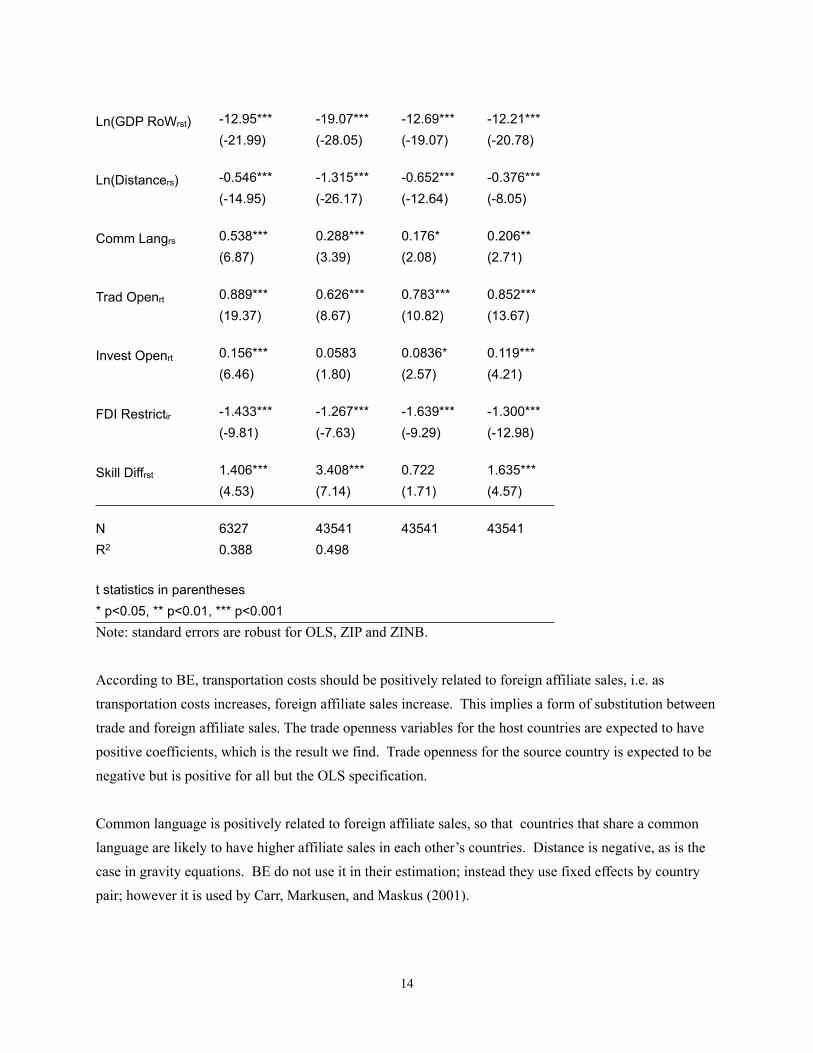
Ln(GDP RoWrst) -12.95*** -19.07*** -12.69*** -12.21*** (-21.99) (-28.05) (-19.07) (-20.78)

Ln(Distancers) -0.546*** -1.315*** -0.652*** -0.376*** (-14.95) (-26.17) (-12.64) (-8.05)

Comm Langrs 0.538*** 0.288*** 0.176* 0.206** (6.87) (3.39) (2.08) (2.71)

Trad Openrt 0.889*** 0.626*** 0.783*** 0.852*** (19.37) (8.67) (10.82) (13.67)

Invest Openrt 0.156*** 0.0583 0.0836* 0.119*** (6.46) (1.80) (2.57) (4.21)

FDI Restrictir -1.433*** -1.267*** -1.639*** -1.300*** (-9.81) (-7.63) (-9.29) (-12.98)

Skill Diffrst 1.406*** 3.408*** 0.722 1.635*** (4.53) (7.14) (1.71) (4.57)

N 6327 43541 43541 43541 R2 0.388 0.498

t statistics in parenthesest statistics in parentheses* p<0.05, ** p<0.01, *** p<0.001* p<0.05, ** p<0.01, *** p<0.001Note: standard errors are robust for OLS, ZIP and ZINB.

According to BE, transportation costs should be positively related to foreign affiliate sales, i.e. as transportation costs increases, foreign affiliate sales increase. This implies a form of substitution between trade and foreign affiliate sales. The trade openness variables for the host countries are expected to have positive coefficients, which is the result we find. Trade openness for the source country is expected to be negative but is positive for all but the OLS specification.

Common language is positively related to foreign affiliate sales, so that countries that share a common language are likely to have higher affiliate sales in each other’s countries. Distance is negative, as is the case in gravity equations. BE do not use it in their estimation; instead they use fixed effects by country pair; however it is used by Carr, Markusen, and Maskus (2001).

14

The two measures of investment barriers: a measure of country-level investment openness from Economic Freedom of the World (EFW), and the OECD measure of sector-level investment restrictiveness. The expected sign on the openness measure is positive: as openness increases, so should foreign affiliate sales. The expected sign on the FDI restrictiveness is correspondingly negative. Our results follow both of these predictions.

The positive coefficient on the capital/unskilled labor ratio implies that firms are more likely to invest in countries that are relatively less skilled labor intensive than themselves, or that a relatively large amount of unskilled labor is attractive to foreign investors.

The trade and investment variables are indicators where a larger number indicates greater openness of the host country. A positive coefficient indicates a positive relationship between openness and foreign affiliate production in the host country. Prior studies do not indicate a clear prediction on the trade variable. Trade may or may not be positively related to foreign affiliate activity (there are theoretical reasons for both a positive and a negative variable, and indeed a non-significant variable). Investment openness is expected to be positively associated with foreign affiliate activity. Interestingly, the only case in which this is true is in the OLS specification, and even in this case the effect is not statistically significant.

In BE, the estimated coefficients are display similar results.10 The coefficients reported by BE are on FDI, not FAS. They do not report regression results on FAS data; however they analyze their model results with respect to both FDI and FAS and find that in most dimensions the two variables respond similarly to changes in model variables. In particular, the signs are the same with the exception of GDP source where our regressions produce the wrong sign, and trade costs for the host country where their regressions produce the wrong sign. The coefficients from BE and from our regressions cannot be quantitatively compared because the two specifications use different measures for trade costs.

As another point of comparison, we examine CMM which has similar analysis to ours. In their case, the model is only a 2 country, 2 factor model, but explicitly considers foreign affiliate sales rather than investment. All of the coefficient results are as predicted by their model.11 There are some differences that make for difficulty in comparing their results with ours. CMM use the sum of the GDPs rather than source and host GDPs. Skill difference is positively related to foreign affiliate sales. Trade costs of host

15

10 The coefficients reported by BE are on FDI, not FAS. They do not report regression results on FAS data; however they analyze their model results with respect to both FDI and FAS and find that in most dimensions the two variables respond similarly to changes in model variables.

11 The variables used by Carr, Markusen, and Maskus (2001) are: the sum of GDPs, the difference of GDPs squared, the skill difference, the interaction of skill difference and GDP difference, investment costs of host, trade costs of host, trade costs of host interacted with squared skill difference, trade cost of source and distance.

countries are positively related to foreign affiliate sales, and investment costs negatively related to foreign affiliate sales. Trade costs of source countries are negatively related to foreign affiliate sales.

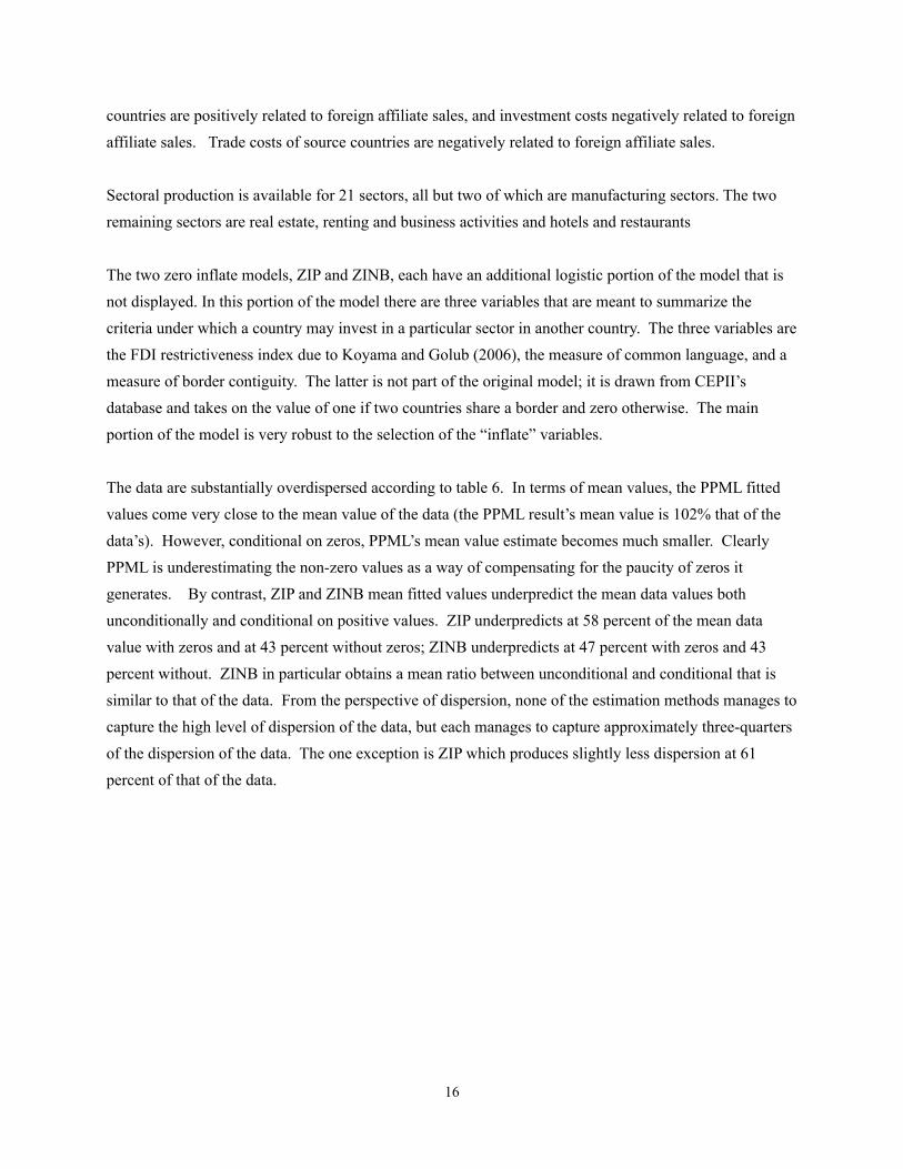
Sectoral production is available for 21 sectors, all but two of which are manufacturing sectors. The two remaining sectors are real estate, renting and business activities and hotels and restaurants

The two zero inflate models, ZIP and ZINB, each have an additional logistic portion of the model that is not displayed. In this portion of the model there are three variables that are meant to summarize the criteria under which a country may invest in a particular sector in another country. The three variables are the FDI restrictiveness index due to Koyama and Golub (2006), the measure of common language, and a measure of border contiguity. The latter is not part of the original model; it is drawn from CEPII’s database and takes on the value of one if two countries share a border and zero otherwise. The main portion of the model is very robust to the selection of the “inflate” variables.

The data are substantially overdispersed according to table 6. In terms of mean values, the PPML fitted values come very close to the mean value of the data (the PPML result’s mean value is 102% that of the data’s). However, conditional on zeros, PPML’s mean value estimate becomes much smaller. Clearly PPML is underestimating the non-zero values as a way of compensating for the paucity of zeros it generates. By contrast, ZIP and ZINB mean fitted values underpredict the mean data values both unconditionally and conditional on positive values. ZIP underpredicts at 58 percent of the mean data value with zeros and at 43 percent without zeros; ZINB underpredicts at 47 percent with zeros and 43 percent without. ZINB in particular obtains a mean ratio between unconditional and conditional that is similar to that of the data. From the perspective of dispersion, none of the estimation methods manages to capture the high level of dispersion of the data, but each manages to capture approximately three-quarters of the dispersion of the data. The one exception is ZIP which produces slightly less dispersion at 61 percent of that of the data.

16

Table 6. Examining the Dispersion of Data and Fitted Values

Foreign affiliate sales Mean ($ million)Standard Deviation

Coefficient of Variation

Datawith zeros 136 1,070 7.87 without zeros 936 2,680 2.86 size difference (without/with) 6.88

OLSwithout zeros 387 857 2.21 percent of Data results 41% 77%

PPMLwith zeros 139 791 5.69 percent of Data results 102% 72%without zeros* 387 821 2.12 percent of Data results 41% 74%size difference (without/with) 2.78

ZIP fitted valueswith zeros 79 380 4.82 percent of Data results 58% 61%without zeros 405 877 2.17 percent of Data results 43% 76%size difference (without/with) 5.13

ZINB fitted valueswith zeros 64 368 5.79 percent of Data results 47% 74%without zeros 401 848 2.11 percent of Data results 43% 74%size difference (without/with) 6.31 *taken to mean without estimates less than 500,000*taken to mean without estimates less than 500,000*taken to mean without estimates less than 500,000

In fact we find very different zeros for data, PPML and ZIP/ZINB. ZIP and ZINB produce the same number of predicted zeros as the logit regression is the same for both. OLS is not displayed as it predicts no zeros. Clearly PPML produces far too few zeros. The ZIP/ZINB values are targeted to the data by selecting the cutoff point that produces the share of zeros observed in the data. There is no theoretical reason to choose a particular cutoff value.

17

Table 7. ZerosSource Positive Values ZerosData 15% 85%PPML 90% 10%ZIP/ZINB 16% 84%

Figure 1. Residuals compared across versions

We perform several tests of the econometric specifications to formalize the preceding analysis. Examining the (negative) log likelihoods generated by PPML, ZIP and ZINB indicates that ZINB is the most preferred out of the three, given that its log likelihood is the smallest.12 Additionally we compute a more specific test to examine whether the ZIP or ZINB proves to be a better fit. The likelihood ratio test for over dispersion between ZIP and ZINB examines whether the estimated mean and variance are equal (as in ZIP) or substantially different (as in ZINB). See Cameron and Trivedi (1998). The LR test yields a result that strongly rejects the null hypothesis that the mean equals the variance.

V. Extrapolation Issues and Modified Estimation StrategyThe results obtained using the theoretical models present certain problems. The variables used in the logistic portion of the zero inflated regressions – the so-called “inflate” variables – present some difficulty in terms of operationalizing the extrapolation of data based on the coefficients produced by the regressions. The regressions described above were based on a set of inflate variables that are known to act as barriers FDI – lack of common language, contiguous borders, and policies that restrict FDI. Although these variables produced estimates that in at least some behave substantially better than either OLS or PPML estimations, a close examination of the logistic portion of the model reveals some peculiarities. The zero inflated methodologies produce thresholds that do not vary sufficiently by country – common language and contiguous borders take the value of one in a minority of the cases. The major variation is across sectors. The clear solution is to add variables that are country specific such as GDP or per capita GDP; however such variables tend to overwhelm the FDI restrictiveness in importance and economic significance; as a result the opposite problem is seen where each country will either receive investment in all of its sectors or receive no investment at all. As a result, despite the promising behavior of the zero inflated models, we proceed with the PPML version of the model.

18

12 We can also examine the consistent Akaike information criterion (CAIC), which in our case presents essentially identical results, as the main difference between the two – adjustments for number of observations and number of parameters – are similar across our models.

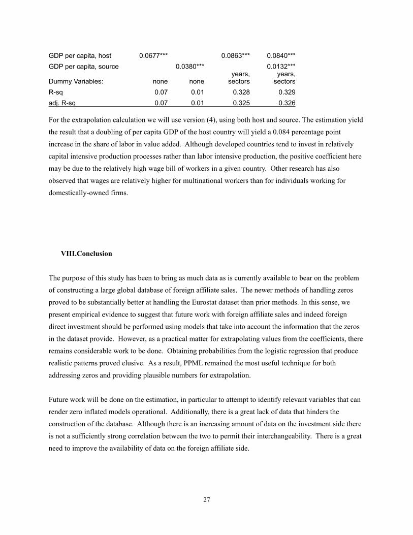
There are further issues, which require other modifications of the model for pragmatic reasons. The econometric model as specified by the theory produces results that are strongly dependent on the size of the source and host country economies. As a result, the extrapolation of the model is strongly influenced by the size of the United States to the point that the vast majority of sales are projected to be sourced from and hosted by the United States. This is despite the presence of other large economies in the sample including Japan (on the source side) and the UK and Germany on both the host and source side. The model clearly fails to take into account the importance of per capita GDP. As a result, we add a GDP per capita variable for both the host and source.13 Under this specification, the econometrics produces results that after extrapolation are substantially closer to data estimates of foreign affiliate sales.

In table 8 below we present three forms of the PPML estimation: the first column reproduces the original PPML specification from table 5. The second column adds the host GDP and the GDP per capita for source and host; the final column eliminates the investment openness variable. For the ultimate extrapolation, we will use column (3)

Several coefficients do change significantly between version (1) and version (3) in table 8.14 The GDP of the source country becomes positive in column (3), which is now in line with expectations; it also an order of magnitude larger than the original estimation in (1). The coefficient on trade openness of the host country becomes negative, in line with a substitution relationship between trade and investment. Skill difference becomes smaller and insignificant (although still positive). Common language and the FDI restrictiveness coefficients are no longer significant, although they remain positive. The GDP RoW coefficient declines substantially in absolute value.

GDP of host, a variable that is usually included in regressions in the literature but that we had left out due to the alternate inclusion of sector level domestic production, is positively associated with foreign affiliate sales, as expected. GDP per capita of the source country is similarly positively associated with foreign affiliate sales; however GDP per capita of the host country is significantly negatively associated with foreign affiliate sales, contrary to usual results of gravity type models.

Table 8. New Estimates (1) (2) (3)

19

13 The investment openness variable was also dropped as it became insignificant and essentially zero after these adjustments.

14 The intermediate columns are versions that use an intermediate mix between the two main specifications, in particular to show (from column (1) to column (2)) the changes made to the original coefficients from adding GDP of host and the two per capita GDP variables. The comparison between (2) and (3) highlights the minimal difference made by removing the investment openness index.

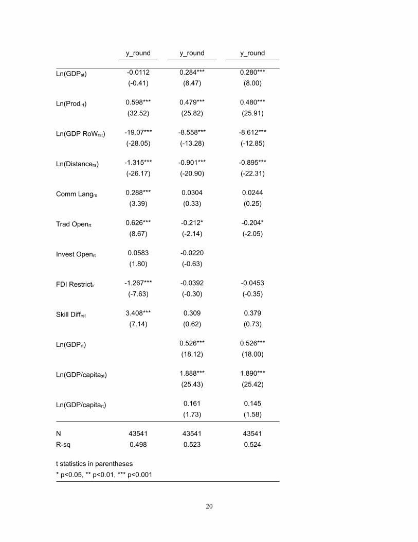
y_round y_round y_round

Ln(GDPst) -0.0112 0.284*** 0.280*** (-0.41) (8.47) (8.00)

Ln(Prodirt) 0.598*** 0.479*** 0.480*** (32.52) (25.82) (25.91)

Ln(GDP RoWrst) -19.07*** -8.558*** -8.612*** (-28.05) (-13.28) (-12.85)

Ln(Distancers) -1.315*** -0.901*** -0.895*** (-26.17) (-20.90) (-22.31)

Comm Langrs 0.288*** 0.0304 0.0244 (3.39) (0.33) (0.25)

Trad Openrt 0.626*** -0.212* -0.204* (8.67) (-2.14) (-2.05)

Invest Openrt 0.0583 -0.0220 (1.80) (-0.63)

FDI Restrictir -1.267*** -0.0392 -0.0453 (-7.63) (-0.30) (-0.35)

Skill Diffrst 3.408*** 0.309 0.379(7.14) (0.62) (0.73)

Ln(GDPrt) 0.526*** 0.526*** (18.12) (18.00)

Ln(GDP/capitast) 1.888*** 1.890*** (25.43) (25.42)

Ln(GDP/capitart) 0.161 0.145 (1.73) (1.58)

N 43541 43541 43541R-sq 0.498 0.523 0.524

t statistics in parenthesest statistics in parentheses* p<0.05, ** p<0.01, *** p<0.001* p<0.05, ** p<0.01, *** p<0.001* p<0.05, ** p<0.01, *** p<0.001* p<0.05, ** p<0.01, *** p<0.001

20

VI. Quadratic Optimization and Final Database

Subsequent to filling in the missing values using econometric extrapolation, final consistency of the database is obtained using a quadratic optimization technique15 that allows us to incorporate and reconcile information from different sources (econometric estimates, OECD, EUROSTAT, BEA and the National Bureau of Statistics of China). This approach parallels that of Boumellassa, Gouel and Laborde (2007).

The objective is to minimize the difference between initial estimates and final values subject to adding up constraints. Thus, for a given sector i, host country r and source country s and reliability weight w, the quadratic optimization is implemented as follows:

(2)

where the FATS0 variables denotes the initial sector/host/source specific foreign affiliates turnover data constructed using the econometric estimates and the raw data collected from OECD, EUROSTAT, BEA and China's NBS. FATS1 denotes the final values resulting from the optimization. Apart from the three-dimensional data we enrich the dataset with information about host and sectoral totals. The constraints of the optimization are aimed to target these aggregate values such as the total global activity of foreign affiliates (), sector/host specific totals (), sector/source specific totals (), bilateral totals () and host and source specific totals ( and ). Reliability weights are chosen such that to reflect our confidence in the correctness of the underlying data. Higher weights increase the penalty for deviating from the initial values and so are used with data in which we have greater confidence; correspondingly, lower weights are used for less certain data. Thus, we confer the highest weights to the EUROSTAT data (w = 100) and the lowest to the econometrically estimated data (w = 1) while data collected from the OECD is given weights of 10. Note that when all weights are equal to one the solution of this model is the constrained least square estimator.

Final Database

The final database has 110 countries and 28 sectors. The extrapolated dataset estimates that approximately 50 percent of global foreign affiliate sales are in manufacturing, while 45 percent are in

21

15 Quadratic optimization has several numerical advantages in implementing very large models relative to cross-entropy minimization techniques (Canning and Wang, 2005).

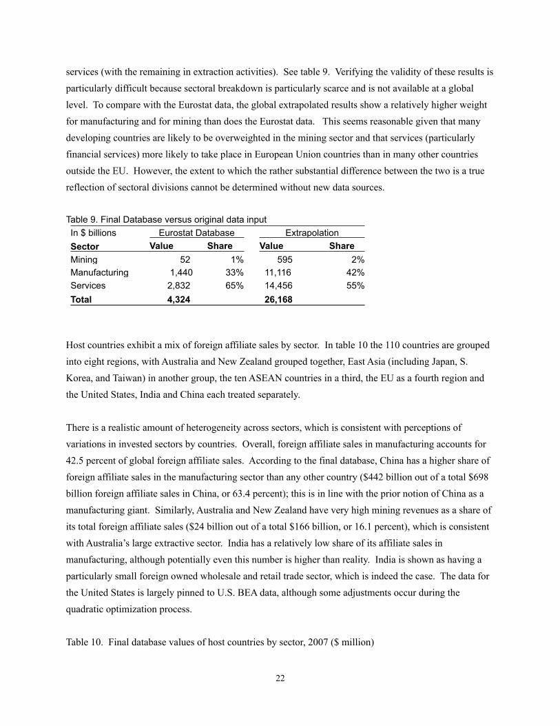
services (with the remaining in extraction activities). See table 9. Verifying the validity of these results is particularly difficult because sectoral breakdown is particularly scarce and is not available at a global level. To compare with the Eurostat data, the global extrapolated results show a relatively higher weight for manufacturing and for mining than does the Eurostat data. This seems reasonable given that many developing countries are likely to be overweighted in the mining sector and that services (particularly financial services) more likely to take place in European Union countries than in many other countries outside the EU. However, the extent to which the rather substantial difference between the two is a true reflection of sectoral divisions cannot be determined without new data sources.

Table 9. Final Database versus original data input In $ billions Eurostat DatabaseEurostat Database ExtrapolationExtrapolationSector Value Share Value ShareMining 52 1% 595 2%Manufacturing 1,440 33% 11,116 42%Services 2,832 65% 14,456 55%Total 4,324 26,168

Host countries exhibit a mix of foreign affiliate sales by sector. In table 10 the 110 countries are grouped into eight regions, with Australia and New Zealand grouped together, East Asia (including Japan, S. Korea, and Taiwan) in another group, the ten ASEAN countries in a third, the EU as a fourth region and the United States, India and China each treated separately.

There is a realistic amount of heterogeneity across sectors, which is consistent with perceptions of variations in invested sectors by countries. Overall, foreign affiliate sales in manufacturing accounts for 42.5 percent of global foreign affiliate sales. According to the final database, China has a higher share of foreign affiliate sales in the manufacturing sector than any other country ($442 billion out of a total $698 billion foreign affiliate sales in China, or 63.4 percent); this is in line with the prior notion of China as a manufacturing giant. Similarly, Australia and New Zealand have very high mining revenues as a share of its total foreign affiliate sales ($24 billion out of a total $166 billion, or 16.1 percent), which is consistent with Australia’s large extractive sector. India has a relatively low share of its affiliate sales in manufacturing, although potentially even this number is higher than reality. India is shown as having a particularly small foreign owned wholesale and retail trade sector, which is indeed the case. The data for the United States is largely pinned to U.S. BEA data, although some adjustments occur during the quadratic optimization process.

Table 10. Final database values of host countries by sector, 2007 ($ million)

22

Mining ManufWholesale/ Retail Transport

Other Services Total

Country share of total

United States 53,361 2,851,463 1,141,805 1,160,649 2,913,562 8,120,840 31.0%China 5,633 442,629 53,276 59,851 136,496 697,886 2.7%India 5,640 119,451 19,101 22,225 55,038 221,454 0.8%E Asia 22,199 1,100,915 264,638 193,272 577,526 2,158,550 8.2%ASEAN 23,599 96,566 156,905 15,612 52,300 344,982 1.3%Aus/NZ 26,826 55,520 35,874 8,767 39,273 166,261 0.6%EU 143,588 4,611,738 2,365,178 612,455 2,815,743 10,548,702 40.3%RoW 314,211 1,837,982 439,734 322,855 994,089 3,908,870 14.9%Total 595,058 11,116,264 4,476,512 2,395,686 7,584,025 26,167,545 Sector share of total 2.3% 42.5% 17.1% 9.2% 29.0%

The largest source countries, as estimated by the final database, are largely in line with expectations. The United States, Germany, United Kingdom, and Japan are all well-known as significant sources of foreign direct investment capital. Norway is estimated to be the third most significant source of foreign direct investment, although that may not be the case in actuality. The host country data shows a similar group of countries, with the France replacing Norway in the top five countries. Japan remains among the top five, which does not conform to expectations as Japan is somewhat uniquely asymmetrical as a large source - but not a large host - of foreign direct investment. More promising, however, is the asymmetry exhibited by China and India, which are currently much more significant hosts of foreign affiliates than sources. China ranks 52nd as a source of foreign affiliate activity, while in 8th place as a host; India ranks 23rd as a host, and in 79th place as a source.

Generally, sources of foreign investment tend to be more concentrated than hosts: certain wealthy, developed countries dominate the ranks of sources of investment, while their investments are scattered broadly across all countries. Although the numbers are close, the final database does not quite exhibit this characteristic. The top five source countries make up 45.percentof all foreign affiliate sales globally; the top 10 make up 66.5 percent. By contrast, the top five host countries make up 58.4 percent of all sales, and the top 10 make up 71.9 percent. Detailed tables for source, host, and sector totals are presented in appendix tables A-6, A-7, and A-8.

Finally, we compare our inward foreign affiliate sales data with Inward FDI stocks obtained from UNCTAD’s World Investment Report data. Comparing foreign affiliate sales with FDI is problematic as they are substantially different objects. Certain issues may weaken the correlation between shares of each of the two variables, such as the relative capital intensity of the investment in particular regions of the world. For example, we might find countries that have large banking sectors such as Luxembourg to be the host to a much higher proportion of global FDI relative to its global share of foreign affiliate sales.

23

Age of the capital installed may also matter; countries that have experienced very recent investments of capital may have not yet realized the full potential in terms of foreign affiliate sales. Finally, countries in which foreign investment is generally made via joint venture or other forms of partial ownership will see high foreign affiliate sales relative to their investment (capital stocks for only their partial ownership is reported, whereas total sales by the affiliate are reported) while a country where 100 percent investments are common would see lower foreign affiliate sales relative to FDI.

These caveats aside, there generally is a positive association between FDI and foreign affiliate sales, and a comparison with FDI may offer some hints as to the appropriateness of the new dataset. It is not necessarily the case that we would expect the same proportions for foreign affiliate sales and FDI; issues that would weaken the association between the two sets of variables. The two sets of data are compared for the eight regions in table 11. The shares exhibit a close correspondence. The largest region, the EU, comprises 40.3 percent of global foreign affiliate sales as host, while also accounting for 39.6 percent of inward FDI stocks. Smaller hosts of foreign affiliate activity – ASEAN, Australia and New Zealand, China and India – each have similarly small shares of inward FDI stocks. East Asia (composed of Japan, Hong Kong, Taiwan and South Korea) is a both a moderately-sized host of foreign affiliate activity and of inward stocks. The major discrepancy lies in the United States and the rest of the world figures; the United States is estimated, in the final database of foreign affiliate sales, to be host to nearly one third of all foreign affiliate sales, while its share of inward FDI is less than one fifth of the global total. The discrepancy is mirrored in the rest of the world figures.

Table 11. Comparison of final database with inward FDI stocks, 2007 ($ millions)

Host CountryFinal databaseFinal database Inward FDI StocksInward FDI Stocks

Host Country Value share Value shareASEAN                  344,982 1.3% 654,614 3.5%Aus/NZ                  166,261 0.6% 453,473 2.4%China                  697,886 2.7% 327,087 1.7%E Asia          2,158,550 8.2% 1,360,001 7.2%EU      10,548,702 40.3% 7,515,798 39.6%India                  221,454   0.8% 105,790 0.6%ROW          3,908,870 14.9% 4,989,185 26.3%United States          8,120,840 31.0% 3,551,307 18.7% Total      26,167,545   18,957,255

Source: Inward FDI Stocks taken from UNCTAD’s World Investment Report, Annex table 3. http://www.unctad.org/Templates/Page.asp?intItemID=5823&lang=1 Accessed 2/29/2012.

VII.Value AddedIn order to have foreign affiliates modeled within GTAP, it is necessary to assign some of the value added of a given sector to the foreign affiliates. In Hanslow (2000), value added is distributed on a pro rata basis

24

to firms under different ownership. There is an extensive literature that indicates this is not the case (see Lipsey 2002 for an overview of this literature). In this section we will specify an estimation equation that will allow us to partition value added into its labor and capital components in a way that includes more detailed information about host and source country as well as by sector.

Value added is calculated by Eurostat as sales less cost of goods sold plus changes in inventories in addition to other adjustments. In addition, Eurostat provides personnel costs, which correspond to the value added of labor.

As with the production data, there are many missing and zero values. A cross-check of the value added data with production data shows that 98.9 percent of the observations are consistent. That is, in 98.9 percent of all observations of value added and production data both show either missing values, zeros, or value data. Because of the high degree of consistency between the two dataset, we rely on the production data to provide information on zeros, and use value added data to focus on the division between labor and capital.

As a second consistency check, we examine the properties of value added and value added of labor. We find that in 98.4 percent of the observations, these two variables produce consistent data. In addition to the criteria mentioned above (i.e. that both variables display missing, zero or non-zero values consistent with one another), the data are checked to see whether total value added is greater than labor value added. This may happen for accounting reasons but cannot be accommodated in the GTAP model. There are a few instances of this, but they occur only in 0.8 percent of all observations.16

The value added ratio is used as the dependent variable. Some summary statistics are listed in table 12.

Table 12. Summary Statistics for Value AddedNumber of host countries 22Number of source countries 41Number of NACE categories (r.1) 115Year coverage 2000-2008

Summary statistics: VA(labor) / VA(total)Summary statistics: VA(labor) / VA(total)Mean 0.593Median 0.605Standard deviation 0.198

25

16 This 0.8 percent is already included in the consistency check that resulted in a 98.4 percent share of consistent data.

Min 0.004Max 0.999

As a first pass, we examine the effects of a series of dummy variables on the value added ratio. We use a plain OLS specification. The specification is as follows:

(3)

The results of this are summarized in table 13.

Table 13. Value added regressions(1) (2) (3) (4) (5)

Dummy Variables used:

Host countries

Source countries Years Sectors All

R-sq 0.176 0.032 0.01 0.218 0.411adj. R-sq 0.176 0.031 0.01 0.215 0.407

There were 28,096 observations in each regression. In the first four regressions, only the specified set of dummy variables is used. Clearly the sector dummy variables and the host dummy variables have substantially greater explanatory power than the other dummy variables.

As a large number of variables are added in the last two regressions both the R2 and the adjusted R2 are presented.

In order to prepare the data set for extrapolation to countries not in the current dataset, we performed regressions using GDP per capita for host and source countries rather than dummy variables. The estimated equation was:

(4)

The results are in table 14.

Table 14. Value added regressions (2)(1) (2) (3) (4)

Independent Variables (log form):

26

GDP per capita, host 0.0677*** 0.0863*** 0.0840*** GDP per capita, source 0.0380*** 0.0132***

Dummy Variables: none noneyears,

sectorsyears,

sectorsR-sq 0.07 0.01 0.328 0.329adj. R-sq 0.07 0.01 0.325 0.326

For the extrapolation calculation we will use version (4), using both host and source. The estimation yield the result that a doubling of per capita GDP of the host country will yield a 0.084 percentage point increase in the share of labor in value added. Although developed countries tend to invest in relatively capital intensive production processes rather than labor intensive production, the positive coefficient here may be due to the relatively high wage bill of workers in a given country. Other research has also observed that wages are relatively higher for multinational workers than for individuals working for domestically-owned firms.

VIII.Conclusion

The purpose of this study has been to bring as much data as is currently available to bear on the problem of constructing a large global database of foreign affiliate sales. The newer methods of handling zeros proved to be substantially better at handling the Eurostat dataset than prior methods. In this sense, we present empirical evidence to suggest that future work with foreign affiliate sales and indeed foreign direct investment should be performed using models that take into account the information that the zeros in the dataset provide. However, as a practical matter for extrapolating values from the coefficients, there remains considerable work to be done. Obtaining probabilities from the logistic regression that produce realistic patterns proved elusive. As a result, PPML remained the most useful technique for both addressing zeros and providing plausible numbers for extrapolation.

Future work will be done on the estimation, in particular to attempt to identify relevant variables that can render zero inflated models operational. Additionally, there is a great lack of data that hinders the construction of the database. Although there is an increasing amount of data on the investment side there is not a sufficiently strong correlation between the two to permit their interchangeability. There is a great need to improve the availability of data on the foreign affiliate side.

27

Appendix

Table A - 1. Source Countries in Eurostat databaseAustralia France Liechtenstein SlovakiaAustria Germany Lithuania SloveniaBelgium Greece Luxembourg SpainBulgaria Hong Kong Malta SwedeCanada Hungary Netherlands SwitzerlandChina (incl. HK) Iceland New Zealand TurkeyCyprus Ireland Norway United KingdomCzech Republic Israel Poland United StatesDenmark Italy PortugalEstonia Japan RomaniaFinland Latvia RussiaSource: Eurostat. Note that Liechtenstein and Luxembourg are excluded from the regression analysis.

Table A - 2. Host Countries in Eurostat databaseAustria Finland Lithuania SloveniaBulgaria France Netherlands SpainCyprus Germany Poland SwedenCzech Republic Hungary Portugal United KingdomDenmark Italy RomaniaEstonia Latvia SlovakiaSource: Eurostat.

28

Table A - 3. Covered SectorsManufacturing Sectors

• Food products, beverages and tobacco*• Textiles*• Wearing apparel; dressing; dyeing of fur*• Leather and leather products*• Wood and wood products*• Pulp, paper and paper products; publishing and printing*• Coke, refined petroleum products and nuclear fuel• Chemicals, chemical products and man-made fibers*• Rubber and plastic products*• Other non-metallic mineral products*• Basic metals*• Fabricated metal products, except machinery and equipment*• Machinery and equipment n.e.c.*• Office machinery and computers*• Electrical machinery and apparatus n.e.c.*• Radio, television and communication equipment and apparatus*• Medical, precision and optical instruments, watches and clocks*• Motor vehicles, trailers and semi-trailers*• Other transport equipment*• Manufacturing n.e.c.*

Other Sectors• Mining and quarrying• Electricity, gas, steam and hot water supply• Collection, purification and distribution of water• Construction• Sale, maintenance and repair of motor vehicles and motorcycles; retail sale of

automotive fuel• Wholesale trade and commission trade, except of motor vehicles and

motorcycles• Retail trade, except of motor vehicles and motorcycles; repair of personal and

household goods• Hotels and restaurants*• Transport, storage and communication• Financial intermediation, except insurance and pension funding• Insurance and pension funding, except compulsory social security• Activities auxiliary to financial intermediation• Real estate, renting and business activities*

Source: Eurostat. Note that * denotes sectors included in the regression analysis.

29

Table A – 4. Eurostat data on foreign affiliate sales by source country.Source Country in $ billions shareUnited States 589 34.6%Netherlands 190 11.2%Germany 187 11.0%France 183 10.8%Switzerland 136 8.0%United Kingdom 102 6.0%Sweden 48 2.8%Italy 40 2.3%Finland 38 2.2%Austria 36 2.1%Japan 32 1.9%Denmark 29 1.7%Belgium 26 1.5%Norway 18 1.0%Spain 16 1.0%Ireland 16 0.9%Canada 4 0.3%Russian Federation 2 0.1%Cyprus 2 0.1%Czech Republic 2 0.1%Israel 1 0.1%Greece 1 0.1%Australia 1 0.1%Portugal 1 0.0%Turkey 0 0.0%Iceland 0 0.0%Hungary 0 0.0%Estonia 0 0.0%Hong Kong 0 0.0%Slovenia 0 0.0%Poland 0 0.0%Romania 0 0.0%Malta 0 0.0%Lithuania 0 0.0%Romania 0 0.0%Slovakia 0 0.0%Hong Kong 0 0.0%Bulgaria 0 0.0%Latvia - 0.0%New Zealand - 0.0%Latvia - 0.0%Total 1,702 100.0%

Note: Data are for 2007 only, and for only observations used in the regressions. Some countries did not report data for 2007.

30

Table A – 5. Eurostat data on foreign affiliate sales by host country.Host country in $ billions shareGermany 579 34%United Kingdom 329 19%Italy 239 14%Netherlands 108 6%Poland 97 6%Sweden 97 6%Austria 73 4%Hungary 65 4%Finland 27 2%Denmark 25 1%Portugal 24 1%Romania 20 1%Slovakia 14 1%Estonia 3 0%Latvia 2 0%Slovenia 1 0%Cyprus 0 0%Total 1,702 100%

Note: Data are for 2007 only, and for only observations used in the regressions. Some countries did not report data for 2007.

31

Table A-6. Final database results by source country (2007)

Rank Source CountryForeign Affiliate Sales (USD m)

Share of World Total Rank Source Country

Foreign Affiliate Sales (USD m)

Share of World Total

1United States 5,510,937 21.1% 56Colombia 7118 0.0%

2Germany 1,824,071 7.0% 57Costa Rica 6527 0.0%

3 Norway 1,581,986 6.1% 58Panama 5707 0.0%

4United Kingdom 1,568,642 6.0% 59South Africa 5089 0.0%

5Japan 1,312,486 5.0% 60Bulgaria 4785 0.0%

6 France 1,239,526 4.8% 61Uruguay 4575 0.0%

7Luxembourg 1,210,800 4.6% 62

Iran Islamic Republic of 4048 0.0%

8Netherlands 1,171,469 4.5% 63Peru 2981 0.0%

9Switzerland 982,593 3.8% 64Belarus 2825 0.0%

10Canada 968,009 3.7% 65Botswana 2603 0.0%

11Ireland 806,119 3.1% 66Thailand 2567 0.0%

12Sweden 752,675 2.9% 67El Salvador 2416 0.0%

13Italy 733,837 2.8% 68Ukraine 2370 0.0%

14Denmark 708,369 2.7% 69Tunisia 2234 0.0%

15Belgium 673,871 2.6% 70Azerbaijan 2006 0.0%

16Austria 588,318 2.3% 71Mauritius 1736 0.0%

17Spain 476,072 1.8% 72Albania 1656 0.0%

18 Finland 449,572 1.7% 73Ecuador 1375 0.0%

19Qatar 433,691 1.7% 74Morocco 1168 0.0%

20Slovenia 419,632 1.6% 75Guatemala 1086 0.0%

21United Arab Emirates 364,572 1.4% 76Namibia 1006 0.0%

22Kuwait 266,320 1.0% 77Armenia 921 0.0%

23 Australia 221,913 0.9% 78Indonesia 791 0.0%

24Korea Republic of 192,262 0.7% 79India 683 0.0%

25Greece 174,105 0.7% 80Honduras 591 0.0%

26Singapore 172,363 0.7% 81Egypt 564 0.0%

27Hong Kong 142,959 0.5% 82Georgia 535 0.0%

28Israel 97,770 0.4% 83Philippines 438 0.0%

29New Zealand 95,517 0.4% 84Paraguay 373 0.0%

32

30Mexico 73,326 0.3% 85Nigeria 297 0.0%

31Portugal 65,016 0.2% 86Bolivia 204 0.0%

32Taiwan 63,719 0.2% 87Sri Lanka 201 0.0%

33Russian Federation 63,568 0.2% 88Mongolia 173 0.0%

34Bahrain 60,991 0.2% 89Nicaragua 164 0.0%

35Cyprus 59,956 0.2% 90Pakistan 139 0.0%

36Saudi Arabia 56,396 0.2% 91Cameroon 124 0.0%

37Slovakia 54,839 0.2% 92Cote d'Ivoire 103 0.0%

38Czech Republic 54,272 0.2% 93Viet Nam 93 0.0%

39Hungary 51,957 0.2% 94Senegal 88 0.0%

40Croatia 41,158 0.2% 95Zambia 52 0.0%

41Estonia 39,011 0.1% 96Kenya 43 0.0%

42Poland 32,397 0.1% 97Ghana 36 0.0%

43Malta 29,635 0.1% 98Kyrgyzstan 33 0.0%

44Lithuania 27,227 0.1% 99Laos 30 0.0%

45Oman 26,892 0.1% 100Cambodia 26 0.0%

46Latvia 26,253 0.1% 101Bangladesh 25 0.0%

47Venezuela 21,484 0.1% 102Tanzania 14 0.0%

48Turkey 20,227 0.1% 103Nepal 11 0.0%

49Brazil 17,884 0.1% 104Uganda 11 0.0%

50Romania 15,973 0.1% 105Madagascar 8 0.0%

51Chile 15,880 0.1% 106Mozambique 8 0.0%

52China 11,842 0.0% 107Ethiopia 6 0.0%

53Argentina 8,462 0.0% 108Zimbabwe 6 0.0%

54Kazakhstan 8,269 0.0% 109Malawi 3 0.0%

55Malaysia 7,782 0.0%

33

Table A-7. Final database results by host country (207)

RankHost Country

Foreign Affiliate Sales (USD m)

Share of World Total Rank Host Country

Foreign Affiliate Sales (USD m)

Share of World Total

1United States 8,120,839 31.0% 56Bulgaria

24,077 0.1%

2United Kingdom 2,362,275 9.0% 57Peru

18,963 0.1%

3Germany 1,848,224 7.1% 58Philippines

18,289 0.1%

4Japan 1,661,741 6.4% 59Slovenia

18,216 0.1%

5 France 1,294,434 4.9% 60Latvia

17,221 0.1%

6Canada 750,910 2.9% 61Pakistan

16,756 0.1%

7Russian Federation 733,341 2.8% 62Tunisia

16,546 0.1%

8China 697,886 2.7% 63Kuwait

15,960 0.1%

9Italy 690,193 2.6% 64Chile

15,685 0.1%

10Switzerland 665,808 2.5% 65New Zealand

15,565 0.1%

11Netherlands 531,004 2.0% 66Estonia

14,224 0.1%

12Spain 517,307 2.0% 67Kazakhstan

13,733 0.1%

13Belgium 501,951 1.9% 68Lithuania

11,785 0.0%

14Mexico 348,738 1.3% 69Cote d'Ivoire

8,018 0.0%

15Korea Republic of 319,675 1.2% 70Ecuador

6,153 0.0%

16Saudi Arabia 306,578 1.2% 71Oman

5,939 0.0%

17Sweden 278,452 1.1% 72Bangladesh

5,589 0.0%

18Austria 265,104 1.0% 73Cyprus

5,441 0.0%

19Poland 256,240 1.0% 74Costa Rica

5,068 0.0%

20Ireland 238,925 0.9% 75Panama

4,572 0.0%

21Turkey 234,656 0.9% 76Azerbaijan

4,462 0.0%

22 Norway 229,571 0.9% 77Bahrain

4,240 0.0%

23India 221,454 0.8% 78Guatemala

3,719 0.0%

24United Arab Emirates 214,158 0.8% 79Sri Lanka

2,672 0.0%

25Brazil 209,900 0.8% 80El Salvador

2,584 0.0%

26Denmark 175,622 0.7% 81Cameroon

2,519 0.0%

27Czech Republic 169,543 0.6% 82Cambodia

2,488 0.0%

28Hungary 166,210 0.6% 83Honduras

2,103 0.0%

29Singapore 161,928 0.6% 84Kenya

1,960 0.0%

34

30 Australia 150,696 0.6% 85Ethiopia

1,843 0.0%

31Croatia 127,104 0.5% 86Uruguay

1,838 0.0%

32 Finland 113,760 0.4% 87Malta

1,611 0.0%

33Romania 103,084 0.4% 88Albania

1,536 0.0%

34Portugal 97,334 0.4% 89Tanzania

1,403 0.0%

35Hong Kong 96,286 0.4% 90Kyrgyzstan

1,401 0.0%

36Iran Islamic Republic of 89,010 0.3% 91Namibia

1,307 0.0%

37Greece 84,479 0.3% 92Ghana

1,254 0.0%

38Taiwan 80,848 0.3% 93Senegal

1,104 0.0%

39Qatar 76,693 0.3% 94Botswana

1,020 0.0%

40Belarus 60,267 0.2% 95Laos

980 0.0%

41Slovakia 51,476 0.2% 96Paraguay

848 0.0%

42Indonesia 49,677 0.2% 97Bolivia

830 0.0%

43Argentina 47,667 0.2% 98Zambia

805 0.0%

44South Africa 45,493 0.2% 99Georgia

788 0.0%

45Israel 44,811 0.2% 100Armenia

715 0.0%

46Luxembourg 44,701 0.2% 101Uganda

664 0.0%

47Thailand 43,533 0.2% 102Nepal

595 0.0%

48Ukraine 43,390 0.2% 103Zimbabwe

583 0.0%

49Egypt 42,707 0.2% 104Nicaragua

506 0.0%

50Malaysia 40,977 0.2% 105Mauritius

493 0.0%

51Venezuela 38,094 0.1% 106Madagascar

385 0.0%

52Colombia 32,977 0.1% 107Mozambique

330 0.0%

53Morocco 30,176 0.1% 108Malawi

281 0.0%

54Viet Nam 27,110 0.1% 109Mongolia

215 0.0%

55Nigeria 24,646 0.1%

35

Table A-8. Final database results by sector (2007)

Rank SectorForeign Affiliate Sales (USD m)

Share of World Total

1Wholesale, retail trade 4,476,512 17.1%2Financial services nec 1,554,060 5.9%

3Construction 1,542,412 5.9%

4Chemical, rubber, plastic products 1,362,150 5.2%

5Transport nec 1,287,882 4.9%

6Business services nec 1,195,440 4.6%

7Petroleum, coal products 1,159,666 4.4%

8Electricity and gas 1,116,839 4.3%

9Motor vehicles and parts 1,085,166 4.1%

10Insurance 1,063,386 4.1%

11Food, bev, tobacco 899,204 3.4%

12Electronic equipment 813,529 3.1%

13Machinery and equipment nec 738,588 2.8%

14Wood products 660,463 2.5%

15Air transport 646,776 2.5%

16Ferrous and nonferrous metals 637,252 2.4%

17Communication 619,904 2.4%

18Manufactures nec 601,492 2.3%

19Coal, oil, gas 595,058 2.3%

20Textiles 576,690 2.2%

21Paper products, publishing 503,919 1.9%

22Water 491,984 1.9%

23Wearing apparel 486,541 1.9%

24Metal products 475,612 1.8%

25Water transport 461,029 1.8%

26Mineral products nec 459,261 1.8%

27Transport equipment nec 407,069 1.6%

28Leather products 249,663 1.0%

36

Bibliography

Anderson, James E. and Eric van Wincoop. 2003. “Gravity with Gravitas: A Solution to the Border Puzzle”. The American Economic Review, Vol. 93(1): 170-192.

Anderson, James E. and Eric van Wincoop. 2004. “Trade Costs”. Journal of Economic Literature,Vol. 42: 691-751.

Blonigen, Bruce A. 2005. “A Review of the Empirical Literature on FDI Determinants.” Atlantic Economic Journal. Vol. 33: 383-403 2005.

Bergstrand, Jeffrey H. and Peter Egger. 2007. “A Knowledge-and-physical-capital Model of International Trade Flows, Foreign Direct Investment, and Multinational Enterprises.” Journal of International Economics. Vol. 73(2): 278-308.

Boumellassa, Houssein ,Christophe Gouel and David Laborde. 2007. “A multisector multicountry FDI database for GTAP,” mimeo.

Cameron, A. Colin and Pravin K. Trivedi. 1998. Regression analysis of count data. Econometric Society Monograph, Cambridge University Press.

Canning, Patrick and Zhi Wang. 2005. “A Flexible Mathematical Programming Model to Estimate Interregional Input–Output Accounts,” Journal of Regional Science, Volume 45, No 3: 539-563.

Carr, David L., James R. Markusen, and Keith E. Maskus. 2001. “Estimating the Knowledge-Capital Model of the Multinational Enterprise.” The American Economic Review. Volume 91, No 3: 693-708.

De Benedictis, Luca, and Daria Taglioni. 2011. “The Gravity Model in International Trade.” In The Trade Impact of European Union Preferential Policies, Ed. Luca De Benedictis and Luca Salvatici. Springer-Verlag.

Fukui, E. Tani, and Csilla Lakatos. 2012. “Measuring Economic Globalization: a Database on the Activities of Foreign Affiliates”, mimeo.

Hanslow, Kevin. 2000. “The Structure of the FTAP Model”. Conference Paper, Third Annual Conference on Global Economic Analysis, Melbourne.

Kleinert, Jörn and Farid Toubal. 2010. “Gravity for FDI.” Review of International Economics, 18(1);1-13.

Koyama, Takeshi, Stephen S. Golub. 2006. “OECD’s FDI Regulatory Restrictiveness Index: Revision and Extension to more Economies.” OECD Working Papers on International Investment, 2006/94, OECD Publishing.

Lipsey, Robert E. 2002. “Home and Host Country Effects of FDI.” NBER Working Paper 9293.

Markusen, James R. “ Trade versus Investment Liberalization.” 1997. NBER Working Paper No. 6231.

Markusen, James R. 2004. “Multinational Firms and the Theory of International Trade.” MPRA Paper 8380, University Library of Munich, Germany.

Markusen, James R. and Keith E. Maskus. 2002. “Discriminating Among Alternative Theories of the Multinational Enterprise,” Review of International Economics. Vol. 10(4): 694-707.

37

Markusen, James R., Anthony J. Venables, Denise Eby-Konan, and Kevin Honglin Zhang. “A Unified Treatment of Horizontal Direct Investment, Vertical Direct Investment, and the Pattern of Trade in Goods and Services.” 1996. National Bureau of Economic Research Working Paper No. 5696.

Martin, Will and Cong S. Pham. 2008. “Estimating the Gravity Model When Zero Trade Flows are Frequent.” Mimeo.

Santos Silva, Joao and Silvana Tenreyro. 2005. “The Log of Gravity.” CEP Discussion Paper No. 701.

Santos Silva, Joao and Silvana Tenreyro. 2011. “Further simulation evidence on the performance of the Poisson pseudo-maximum likelihood estimator.” Economic Letters. Vol. 112: 220-222.

Yeaple, Stephen Ross. 2003. “The Role of Skill Endowments in the Structure of U.S. Outward Foreign Direct Investment.” The Review of Economics and Statistics. Vol. 85 (3): 726-734.

38