A GIS framework for spatio-temporal analysis and visualization of

laboratory mice tracking data

Mareike Kritzler, Martin Raubal, Antonio Krüger

Institute for Geoinformatics

University of Münster

Abstract

Knowing the locations and spatio-temporal paths of individual mice is an essential

prerequisite for behavioral analysis of large groups of laboratory mice. Traditional

observations have been carried out by trained humans who are able to distinguish more than

fifty behavioral patterns. This is a tedious labor limited with respect to observation length. In

this paper we propose a tracking solution based on the integration of GIS and RFID (Radio

Frequency Identification) technology to automatically collect 24h/7days of movement data.

Appropriate cage design and antenna placement are discussed. A software solution is

presented to facilitate the recording (JerryTS), visualization and analysis (TOM) of mice

movements.

1. Introduction

The motivation behind this work is to observe the behavior and movement of laboratory mice

in a large indoor semi-natural environment (SNE) measuring 1.75 by 1.75 by 2.1 m (L x W x

H) (Figure 1). In this case biologists want to detect differences between mice carrying a

genetic disposition to develop Alzheimer-like pathology and their wildtype conspecifics under

semi-natural conditions. The SNE contains several floors connected by small bridges and

ropes that allow the mice to establish a complex social system comprising different territories.

Figure 1 SNE without antennas

Previously, data has been collected manually by observers sitting in front of this complex

cage. The observers are thoroughly trained in behavioral biology and can differentiate up to

55 unique behavioral and movement patterns. The population is allowed to grow up to a size

of 40 adult mice (plus their offspring), who are individually marked using a color coding

scheme on their tails and ears. The resulting data gets analyzed statistically to investigate mice

behavior.

There are, however, disadvantages regarding the manual recording of animal behavior: The

performance of a single human observer varies to some degree constrained by fatigue or

mood, and different observers may introduce a specific bias to the recording process

(Lewejohann et al. 2006). Furthermore, some information (e.g., accurate metric measures) can

not be gained by analogue observation of an animal. Human observation is also limited with

respect to observation length, making it difficult to gain long-term data (e.g., 24 hour

observations). Moreover, data collection during the night-phase is challenging due to the

difficulties of identifying color-marked mice in the dark (it is important to consider that mice

are nocturnal animals).

The motivation behind the introduction of an automatic RFID-based tracking system and GIS

framework for laboratory mice is to improve and extend human observations. The aim of this

research is therefore to establish a system, which automatically tracks, visualizes and analyses

spatio-temporal data of a large number of individual subjects over a long period of time.

The integration of RFID technology in the SNE requires some modifications to the original

cage design. The enclosure is equipped with ring antennas placed at strategically chosen

spots. The challenge is finding a hardware setup and cage design which allow collecting

consistent data and retain the semi-natural character of the cage. Furthermore a new software

solution must be developed in order to show the positions of the mice at certain times in the

cage and to allow several analyses of mice behavior.

Section 2 presents the base technology and the methods used in this work. In Section 3 we

introduce the test environment and application scenario – laboratory mice in a semi-natural

environment. Section 4 describes and specifies the two main software solutions developed for

automatic animal tracking, and the analysis and visualization of the resulting data. Section 5

discusses the results of applying the software prototype to the test environment. The paper

finishes with conclusions and directions for further work.

2. Technology and Methods

Before specifying and implementing the automatic tracking, visualization, and analysis

system for laboratory mice it is necessary to give some background information about the

used RFID technology and concepts from time geography.

2.1 Technology

As mentioned before the collecting of data has previously been done by visual observation.

Different technologies are in use to automate data collection in the fauna. For example, the

movement behavior of Antarctic fur seals is observed by satellite transmitters. Three satellites

were used providing a positional accuracy of 150 m to determine the tracks of the animals

(Bonadonna et al. 2000). Cows are tracked in their barn using radar technology. Transmitters

are fixed at the neckband of the cows, allowing a 2D localization with an accuracy of 25 cm

(Neisen 2005). These tracking techniques do not fit the requirements for indoor mice tracking.

GPS (Global Positioning System) is inappropriate for indoor tracking because of lacking

visibility of satellites (Leick 1995). The radar technique is not useful because mice cannot

wear large transponders. Both technologies also fail with regard to the accuracy requirements

for the presented work.

The RFID technology for the tracking of the mice is chosen because the passive transponders

are very small and therefore easy to inject into the mice. The installation of the antennas in the

SNE is possible and accurate positional data can be achieved. RFID technology has been

successfully applied in various domains. For example, RFID chips were used during the

soccer World Cup 2006 in Germany for entrance controls. Such technology makes it also

possible to track visitors and support them in their wayfinding tasks, e.g., from the parking lot

to theirs seats in the stadium (Tomberge and Raubal 2006). RFID was also used to improve

the position of mobile robots and persons in their environment: With RFID tags it is possible

to create maps using mobile platforms that are equipped with RFID antennas which assist

localization (Hähnel et al. 2004). RFID technology can be used to collect environmental data

and build up a Bayesian network for positioning (Brandherm and Schwartz 2005).

2.2 Methods

Data collected with RFID have a spatial and a temporal dimension. The visualization and the

analysis of the data must reflect the time-variant position in space. In time geography human

activities have been the focus within an effort to define the space-time mechanics. Thereby

human activity patterns and movement in space and time are analyzed. Individual activities

and movements are continuous sequences in geographical space. The number and places of

activities of one person during a day are limited by time-geographic constraints (Kwan 2004).

Presence of other people and rules in a community restrict a person’s potential actions. The

constraints can be divided into (Hägerstrand 1970):

• Capability constraints: activity and movement radius are limited because of biological

conditions such as eating or sleeping;

• coupling constraints: refer to the requirement for a person to be at a specific location

at a certain time or for a fixed time duration;

• authority constraints: things or events are controlled by certain individuals or groups.

An individual describes a path in a space-time framework, which reaches from the point of

birth to the point of death. The concept of a life path can be graphically visualized: the three-

dimensional space is shown in a two dimensional plane und the perpendicular describes the

time (Hägerstrand 1970). Space-time paths and space-time prisms demonstrate two central

concepts for visualization and analysis of movement patterns in time geography (Miller

2005).

• Space-time path:

Space-time paths depict the movement of individuals in space over time. Such paths

are available at various spatial (e.g., house, city, country) and temporal granularities

(e.g., decade, year, day) and can be represented through different dimensions. Figure 2

shows a person’s space-time path during a day, representing her movements and

activity participation at three different locations. The slope of the path represents the

travel velocity. If the path is vertical then the person is engaged in a stationary activity.

Figure 2 Space-time path

• Space-time prism:

All space-time paths must lie within space-time prisms. These are geometrical

constructs of two intersecting cones (Lenntorp 1976). Their boundaries limit the

possible locations a path can take based on people’s abilities to trade time for space. In

order for a person or activity to be accessible, its space-time station must intersect the

space-time prism for a minimal temporal duration. Figure 3 depicts a space-time prism

for a scenario where origin and destination have the same location. The time budget is

start

time

space stop finish

defined by ∆t = t2−t1 in which a person can move away from the origin, limited only

by the maximum travel velocity.

Figure 3 Space-time prism

Time geography has been applied in the area of GIS regarding transportation networks to

model and measure space-time accessibility (Miller 1999, Miller and Wu 2000; Wu and

Miller 2001). It has also been advocated to integrate time geography with both GIS and

Location-Based Services to achieve more user-centered systems (Raubal et al. 2004; Miller

2005). Further applications in the geo-domain concern the structuring of dynamic wayfinding

environments (Hendricks et al. 2003) and the modeling of geospatial lifelines (Hariharan and

Hornsby 2000). Analytical formulations of basic entities and relationships from time

geography can be found in (Miller 2005a). A space-time web model—a display of life paths

which underlie the time-geographic constraints—can be applied to all aspects of biology to

vary from flora over fauna to humans (Hägerstrand 1970).

3. Test environment and application

To get the data for movement and behavior of the mice an RFID system (Trovan Electronic

Identification Systems) consisting of reader (LID 665 Miniature OEM Board), ring antennas

time

space

(air-core coil antenna for LID 665) and animal glass transponders (ID 100) are used. The mice

are individually marked with these small (12 mm length, 2 mm diameter) passive integrated

transponders (PIT) that are injected subcutaneously between the scapulas. The IDs of

individual animals can be read while traversing the electromagnetic field, which is established

by the ring antennas, e.g. when passing through tubes or visiting drinking places.

Figure 4 Schematic view of the SNE (top and front)

In the setup the minimum distance between two antennas is 20 cm (Figure 4). Transponders

are read within a 0.5 cm distance, therefore mice do not necessarily have to move over

antennas. The readers are able to read several transponders at the same time at a maximum

rate of 26 Hertz.

In order to receive meaningful data describing the movement of mice, some structural

changes must be considered and realized in the SNE, constraining the mice to pre-defined

pathways. The cage is restructured to get information about the mice regarding changes of

floors, movement across floors, directions of movement, home ranges of individuals, drinking

and emigration behavior. To gather those data the cage is realized as follows: The SNE is

1,75 m

1,75 m

40 x 40

40 x 40

40 cm

60 cm

80 cm

1,75 m

2 m

divided into five areas (Figure 5). The ground is divided by a wall into two sections and there

are 3 floors on different levels which are connected by sloping tubes and a rope. Outside the

SNE an emigration cage is provided, which can be accessed from the ground floor (i.e., to

give shelter to low-ranking animals within the group hierarchy) via a tube and crossing a

water basin. To get reasonable data the antennas are placed at strategically chosen spots, i.e.,

where the mice must cross. Every Plexiglas tube has two antennas at the beginning and end,

therefore it can be detected when a mouse changes the floor, in which direction mice cross the

tubes and also the velocity of mice.

Figure 5 Schematic view of SNE with antennas

In every area there is an antenna beneath the drinking bottle to get data about the drinking

behavior and to establish a warning system when a mouse does not drink. Additionally, every

area contains a tube supplied with two antennas, enabling the collection of data about the

movement on the floors and possible dominance relationships. In total there are 27 antennas

drinking bottle

emigration cage

drinking bottle

drinking bottle

drinking bottle

drinking bottle

water basin

integrated in the SNE (see Figure 6). With this design it is possible to collect the necessary

data about movement and behavior.

Figure 6 SNE with antennas

4. Software Solutions: JerryTS and TOM

To establish an automatic tracking, visualization and analysis system for laboratory mice it is

necessary to develop a software solution, which collects, stores, manages, and supplies the

data and visualizes the derived information.

4.1 JerryTS (Database management for RFID-based events)

To configure the RFID readers and to handle the reading of transponder codes a software

called JerryTS has been developed using the programming language Java. If a mouse enters

the electromagnetic field of the antenna the transponder code is read by the RFID reader,

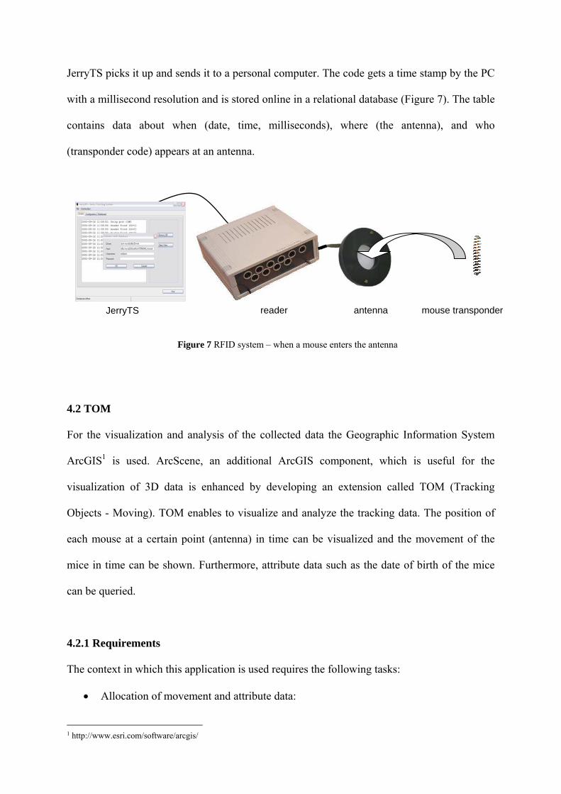
JerryTS picks it up and sends it to a personal computer. The code gets a time stamp by the PC

with a millisecond resolution and is stored online in a relational database (Figure 7). The table

contains data about when (date, time, milliseconds), where (the antenna), and who

(transponder code) appears at an antenna.

4.2 TOM

For the visualization and analysis of the collected data the Geographic Information System

ArcGIS1 is used. ArcScene, an additional ArcGIS component, which is useful for the

visualization of 3D data is enhanced by developing an extension called TOM (Tracking

Objects - Moving). TOM enables to visualize and analyze the tracking data. The position of

each mouse at a certain point (antenna) in time can be visualized and the movement of the

mice in time can be shown. Furthermore, attribute data such as the date of birth of the mice

can be queried.

4.2.1 Requirements

The context in which this application is used requires the following tasks:

• Allocation of movement and attribute data:

1 http://www.esri.com/software/arcgis/

JerryTS antenna reader

Figure 7 RFID system – when a mouse enters the antenna

mouse transponder

The database filled with attribute and movement data collected by JerryTS must be

connected to the new software. The data must be prepared for further processing so

that redundant data can be aggregated and illegal transponder codes found.

• Digitizing of the data sources:

The data for the visualization and analysis must be created. The SNE with the different

floors, the antennas and the dynamically moving mice must be digitized to scale. Such

graphical data are required for the visualization.

• Visualization of movement and behavior data:

The created digital data must be visualized in three dimensions. Visualization of the

SNE and the antennas should not change, the position of the mice must be adapted to

the movement in time. The mice in the SNE have to be listed so that specific subjects

can be chosen for visualization and analysis. They should be displayed for a certain

time interval with different temporal resolutions and colored depending on gender.

The presentation must point out whether a position of a mouse is approximated or

based on a database entry. Analyses and statistics must be clearly represented.

• Analysis of movement and behavior data:

An automated analysis function should query the attribute data (e.g. gender or day of

birth) of selected mice and statistics about behavior, i.e., analysis per day and per

level.

• The data export must be in a generally accepted format to be used with other software

solutions.

4.2.2 Modeling

Before the software extension can be implemented, the data base must be created with the

existing software solutions ArcCatalog (to manage and create the necessary files and data

structures) and ArcMap (to digitize the cage). To store the data a PGDB (Personal

Figure 8 Data base created in ArcMap

Geodatabase) in ArcCatalog is built. For this purpose a feature dataset is created. Therefore a

coordinate system (local Cartesian projection) is developed that fits to the large scale. In the

feature dataset the model of the SNE is created. Every level is represented by feature class

with the corresponding attributes, so the layers can be handled separately. The RFID antennas

and tubes are realized as a geometric network with nodes and edges containing different

weights for the analysis. To visualize and analyze the mice a further feature class stores

mouse objects with the necessary attributes.

All time invariant components of the setting are digitized in ArcMap (Figure 8). Those are the

levels, the positions of the antennas and the ways between the antennas. The dot features

representing the mice are created in the program dynamically because they do not have a

fixed position. The spatial resolution is in centimeters.

4.2.3 Implementation

The prototypical implementation of the ArcScene extension is done with ArcObjects and the

programming language C#. First the database connection to the extension is realized.

Figure 9 Program flow of TOM

The data base consists of two tables: one with the time and movement data (collected by

JerryTS) and the second with the mice attribute data (Figure 9). TOM is implemented by the

MVC (Model View Controller) pattern (Krasner and Pope 1988) with three packages (Figure

10):

• Model: Data base

• Controller: Distribution and algorithms

• View: GUI-elements

Beyond this package structure there exists the superior class “TOM” which represents the

whole extension.

ODBC TOM

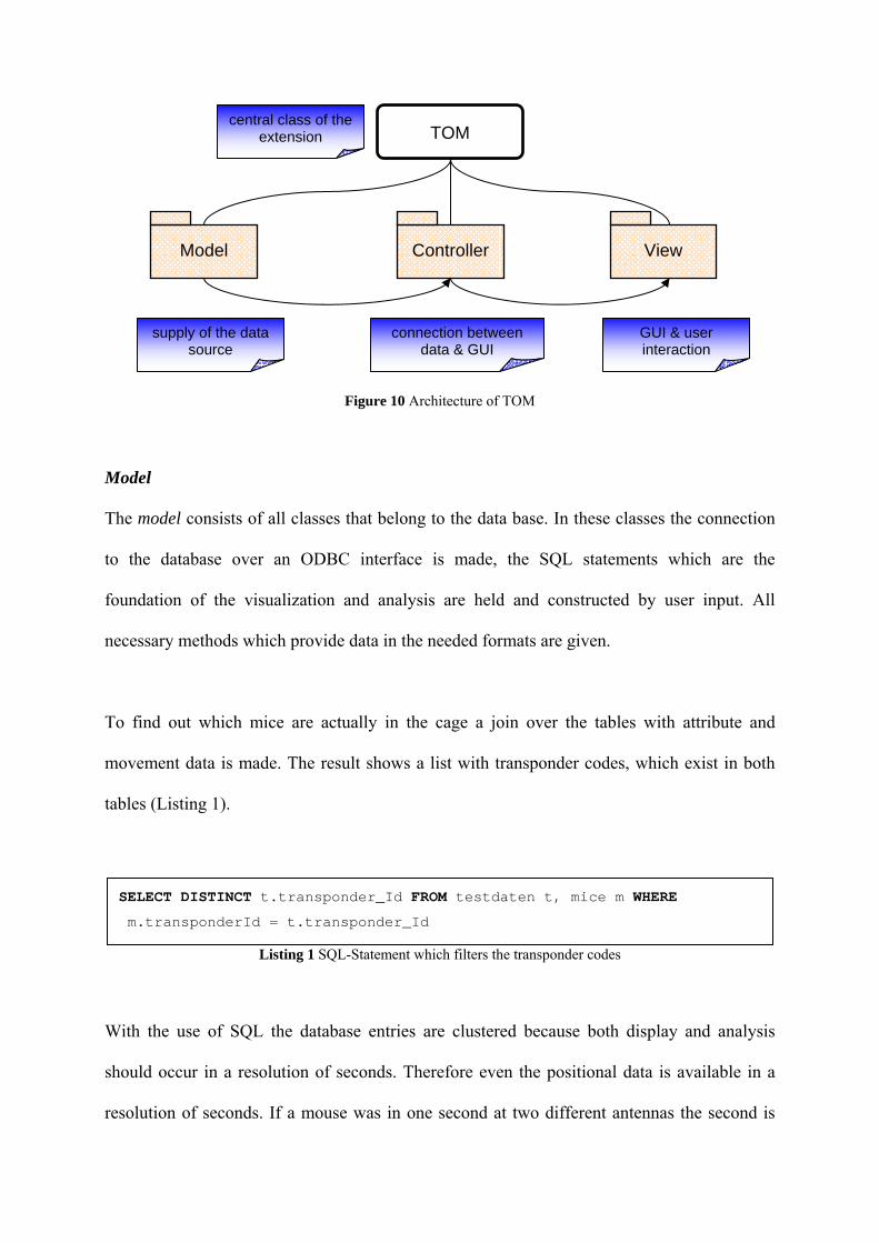
Figure 10 Architecture of TOM

Model

The model consists of all classes that belong to the data base. In these classes the connection

to the database over an ODBC interface is made, the SQL statements which are the

foundation of the visualization and analysis are held and constructed by user input. All

necessary methods which provide data in the needed formats are given.

To find out which mice are actually in the cage a join over the tables with attribute and

movement data is made. The result shows a list with transponder codes, which exist in both

tables (Listing 1).

Listing 1 SQL-Statement which filters the transponder codes

With the use of SQL the database entries are clustered because both display and analysis

should occur in a resolution of seconds. Therefore even the positional data is available in a

resolution of seconds. If a mouse was in one second at two different antennas the second is

TOM central class of the

extension

supply of the data source

connection between data & GUI

GUI & user interaction

Model View Controller

SELECT DISTINCT t.transponder_Id FROM testdaten t, mice m WHERE

m.transponderId = t.transponder_Id

dissolved into milliseconds. Both positions are stored in the database and no positional

information in lost (Listing 2).

Listing 2 Statement for clustering of positional data

To manage the mice a separate future class is needed, which represents the mice with their

attribute data (Figure 11). A mouse object is created when a mouse should be displayed but

does not exist. Whenever the program is started, all mouse features of a previous session get

deleted.

Figure 11 Data model for the mice

SELECT unit, datum, zeit, millis FROM testdaten t WHERE transponder_Id = ’00066AC0D3’ AND datum = ’2005-10-27’ AND zeit >= ’16:36:27’ GROUP BY zeit, unit, ORDER BY zeit, millis

Controller

Classes in the controller provide methods, which allow communication between model and

the graphical user interface (GUI), realize the time component in the extension and enable

analysis. The management of time is realized with a timer. Through the start of the timer it is

verified whether the selected mice exist. If a mouse object does not exist, a new one is created

and depending on the gender colored in blue or red. At every tick of the timer a data

structure—filled by the database—is queried with regard to whether positional data for every

displayed mouse is available. When an entry is found the position of the corresponding

antenna is read and assigned to the mouse object. The mouse then “jumps” from antenna to

antenna. If there are there two positional entries for one second the mouse moves from the

first to the second position. If there is no entry in the data structure the color of the mouse at

its last position changes to indicate that data are not “live” but only approximated.

TOM provides statistical functions for analysis of the collected data. The analysis is divided

into statistics per day and per level (Table 1). Analysis per day shows the last time stamp of

drinking and weighting, the number of antenna contacts and the number of used levels. The

two last variables are indications for the agility of mice. Analysis per level provides

information about the duration of stay per level, the count of antenna contacts and whether a

mouse stays alone on the level or if other mice have been present.

Table 1 Analysis functions

Analysis per day Analysis per level

Time of last drinking Number of antenna contacts

Time of last weighting Duration of stay

Number of antenna contacts Stay with other mice

Number of used levels

As an example for the analysis, we describe the functionality of the algorithm calculating

whether a mouse stays at a certain date alone on a level or not (Listing 3).

Listing 3 Pseudo code of the method “contactToOtherMiceOnLevel”

The method “contactToOtherMiceOnLevel” which returns an array with Boolean values has

two parameters: the selected mouse and the date for which the information is queried (line 1).

In line 2 to 5 necessary attributes are declared and initialized: the array which will be returned

as result is initialized with the Boolean value ‘false’ for each level (line 2). The clustered data

for one day (contacted antennas und timestamps) of the other unselected mice are stored in an

array “miceWithoutSelected” (line 3). The number of the antenna where the selected mouse

has the first contact at this date and the time of this contact are recognized (line 4 and 5).

First the changes of levels for the selected mouse must be detected (lines 6-9). Therefore the

antennas were associated with the corresponding levels before. Now the list

“antennaTimeArray” (antenna and time data) of the selected mouse is scanned until an

// returns an array with Boolean which show whether a mouse had contact to other mice per level 1 contactToOtherMiceOnLevel bool[] (String mice, String currentDate){ 2 bool[] levelsMeet ={false,false,false,false,false,false}; 3 String[]miceWithoutSelected; //array with all unselected mice 4 String antennaStart; //number of start antenna 5 Date timeStart //time of contact with antennaStart 6 for(i = 1; i < antennaTimeArray; i++){ 7 String antenna = antennaTimeArray[i][0]; 8 if(antennaStart and antenna not on the same level){ 9 findLevelWhereMouseIs(); 10 DateTime time = antennaTimeArray[i-1][1]; //last time on 11 level 12 if(two mice on one level){ 13 getTimeFromDB&AntennasForUnselectedMice; 14 if(unselectedMiceOnLevelWithMice){ 15 set levelsMeet corresponding of true; 16 timeStart = time; 17 antennaStart = antenna; 18 } 19 } 20 } 21 return levelsMeet; 22 } 23 }

antenna is found which is not derived from the same level like “antennaStart“ (line 8). If a

change of level is found, we know the current level (line 9) and the time interval when the

mouse was on this level (line 10). In line 13 it is verified whether an antenna entry of an

unselected mouse for this time interval exists:

• If an antenna entry of an unselected mouse exists, all entries in the list

“miceWithoutSelected” are checked if the antennas are from the same level like

antenna start (line 14):

o If the antennas are from the same level, the corresponding Boolean attribute for

the level becomes true (line 15). That means the selected mouse has contact to

another mouse at this date on this level.

o If the antennas are not from the same level, nothing happens and the loop starts

again: antenna start gets the first antenna of the next level as new value and the

next change of level will be detected (go to line 6).

• If no antenna entry of an unselected mouse in the time interval exists in line 13, the

loop starts again, the start antenna gets first antenna of the next level as new value and

the next change of level will be detected (go to line 6).

The algorithm ends when the list “antennaTimeArray” is completely traversed and all

possible level changes are detected.

It is possible to export the data for statistical analyses with other software. The data is derived

from two underlying database relations: one table with the tracking data filled by JerryTS and

a second table where attribute data of the mice are stored. In addition, a warning system is

established, to detect when a mouse has not been drinking for a longer time period or using

the emigration cage.

View

The view package contains all classes which belong to the GUI. The list of mice and the user

input are connected to one GUI element. Furthermore there are classes for the toolbar, menu

and dialogs.

Figure 12 Screenshot TOM

To start the extension the toolbar is used. After the start the database connection must be

established and the data base of the SNE must be chosen. The list of the mice is automatically

loaded (Figure 12). If mice are selected, the visualization of the attribute data as well as the

display of mice is possible.

5. Results and discussion

The software JerryTS configures the RFID readers and stores the read transponder codes in an

RDBMS. One table of the database stores the transponder codes with the number of the reader

with date, time and milliseconds. The system provides an ID so the dataset can be identified.

Every dataset is unique, for every timestamp there exists only one database entry.

Figure 13 Attribute dialog of attribute data stored in the database

The software TOM allows to visualize attribute data und motion sequences and to perform

statistical analyses of the collected data. It is possible to query attribute data of selected mice

from the centrally managed attribute table and to view them in a table (Figure 13).

The position of selected mice inside the SNE can be displayed. For the visualization a time

interval must be chosen. During this interval the mice move in different display speeds and in

different play back rates. The time-variant position can be tracked through the visualization

sequence (Figure 14). A chosen mouse describes a space-time path and by means of this the

activity and movement patterns can be derived. The spatial component is displayed in three

dimensions, the temporal component is realized through the clock in the GUI. Through the

proposed solution in milliseconds an accurate representation of the data is possible: if during

one second, a signal of the same mouse is registered at two antennas—when antennas are

directly connected through a tube—a linear movement is displayed.

Figure 14 Sequence of mouse movement in time

The results of the prototypically implemented analysis are displayed in the shown statistics

dialog (Figure 15). It gives a list of all mice in the SNE. By selecting one mouse all necessary

data are queried and handled by the described algorithms. Figure 15 illustrates mouse

00066AB37B at 22.2.2006 with its statistics. It is shown that this mouse used all five areas

but no meeting with other mice occurred. The tables in this dialog can be exported and serve

as the data base for both visualization and analysis. The upper table contains the clustered

data, the lower table contains the antenna contacts per minute.

24.02.2006 16:38:34 405 ms

24.02.2006 16:38:35 176 ms

24.02.2006 16:38:48 165 ms

24.02.2006 16:38:48 515 ms

Figure 15 Statistics dialog

The warning system shows in the GUI whether and how many warnings exist. A dialog

displays the warning messages which have a timestamp and the transponder code. A warning

appears if there is no antenna contact at a drinking bottle within a day or the emigration cage

is used.

6. Conclusions and future work

In this paper we presented an indoor-tracking solution for laboratory mice. The use of RFID

technology facilitates the collection of time continuous movement data in a complex

biological scenario. Twenty-four hour observation is possible without disturbing the animals.

Social interaction and the outward appearance are not influenced by this technology and only

a few modifications must be made to integrate the RFID antennas in the SNE. The software

JerryTS collects the data and provides the data base for further analysis. The novel approach

was integrated within a GIS framework by extending the software component ArcScene. This

extension (TOM) was used to handle the spatio-temporal data. On the one hand the movement

of the mice is visualized and on the other hand there are analysis functions, which offer

information about the behavior and movement of the mice.

The described setting can be extended by using additional sensors, e.g., a scale to measure

data about weight and more continuous positional data, not only point data at the antennas.

Optical camera tracking is considered for tracking single mice to get additional behavior

patterns. Furthermore it is possible to integrate an automated learning test for the mice. The

analysis can be extended to filter behavior and movement patterns to be used in various

biological behavior studies. We also consider to create a framework which allows to get

tracking data of different kinds of animals in different temporal and spatial resolutions.

Acknowledgments

We would like to thank Norbert Sachser, Lars Lewejohann and their colleagues at the

Department of Behavioral Biology at the University of Münster. They offered us the

opportunity to work with the laboratory mice in the SNE, provided us with the hardware and

supported us with their knowledge about laboratory mice.

References

Bonadonna, F., M.A. Lea, C. Guinet, (2000). Foraging routes of Antarcic fur seals

(Arctocephalus gazella) investigated by the concurrent use of satellite tracking and time-

depth. Polar Biol (2000) 23: 149-159. Springer 2000.

Brandherm, B. and T. Schwartz, (2005). Geo Referenced Dynamic Bayesian Networks for

User Positioning on Mobile Systems. In Proceedings of International Workshop on

Location- and Context-Awareness (LoCA), Munich, Germany.

Hägerstrand, T. (1970). What about people in regional science? Papers of Regional science

Association 24: 7-21.

Hähnel, D., W. Burgard, D. Fox, K. Fishkin, M. Philipose (2004). Mapping and Localization

with RFID Technology. In Proceedings of the IEEE International Conference on Robotics

and Automation (ICRA).

Hariharan, R. and K. Hornsby (2000). Modeling Intersections of Geospatial Lifelines. in: First

International Conference on Geographic Information Science, GIScience 2000, Savannah,

Georgia, USA.

Hendricks, M., M. Egenhofer, K. Hornsby (2003). Structuring a Wayfinder's Dynamic Space-

Time Environment. in: W. Kuhn, M. Worboys, and S. Timpf (Eds.), Spatial Information

Theory - Foundations of Geographic Information Science, International Conference,

COSIT 2003, Kartause Ittingen, Switzerland, September 2003. Lecture Notes in Computer

Science 2825, pp. 75-92, Springer, Berlin.

Kwan, M-P. (2004). GIS Methods in Time-Geographic Research Geocomputation and

Geovisualization of Human Activity Patterns. Geogr. Ann. Swedish Society for

Anthropology and Geography. 86 B(4): 267:280.

Krasner, G. and S. Pope (1988). A Cookbook for Using the Model-View-Controller User

Interface Paradigm in Smalltalj-80. JOOP August / September 1988, 26-49.

Leick, A. (1995). GPS - Satellite Surveying. Wiley, New York.

Lenntorp, B. (1976). Paths in Space-Time Environments: A Time-Geographic Study of the

Movement Possibilities of Individuals. Lund Studies in Geography, Series B (44).

Lewejohann, L., C. Reinhard, A. Schrewe, J. Brandewiede, A. Haemisch, N. Görtz, M.

Schachner, N. Sachser (2006). Environmental Bias? Effects of Housing Conditions,

Laboratory Environment, and Experimenter on Behavioral Tests. Genes Brain and

Behavior 5: 64-72.

Miller, H. (1999). Measuring space-time accessibility benefits within transportation networks:

Basic theory and computational methods. Geographical Analysis 31: 187-212.

Miller, H. (2005a). A Measurement Theory for Time Geography. Geographical Analysis

37:17-45. The Ohio State University.

Miller, H. (2005). What about people in geographic information science? in: P. Fisher and D.

Unwin (Eds.), Re-Presenting Geographical Information Systems. pp. 215-242, John Wiley.

Miller, H. and Y.-H. Wu (2000) GIS software for measuring space-time accessibility in

transportation planning and analysis. GeoInformatica 4:141-159.

Neisen, G. (2005). Validation of a local positioning monitoring system (LPM) in relation to

dairy cow behavior. Second Annual Symposium of the PhD-Programme for Sustainable

Agriculture ASPSA 2005.

Raubal, M., H. Miller, S. Bridwell (2004). User-Centred Time Geography For Location-

Based Services. Geografiska Annaler B 86(4): 245-265.

Tomberge, P. and M. Raubal (2006). Navigation mittels RFID - Untersuchung der

Navigationsmöglichkeiten durch RFID-Eintrittskarten bei der Fussball-WM 2006. in: J.

Strobl and C. Roth (Eds.), GIS und Sicherheitsmanagement. pp. 91-100, Wichmann,

Heidelberg.

Wu, Y.-H. and H. Miller (2001). Computational tools for measuring space-time accessibility

within dynamic flow transportation networks. Journal of Transportation and Statistics

4(2/3): 1-14.