A genetic algorithm for robotic assembly line balancing · A genetic algorithm for robotic assembly line balancing Gregory Levitin a,*, Jacob Rubinovitz b, Boris Shnits b a DivisionofPlanning,DevelopmentandTechnology

ARTICLE IN PRESS

European Journal of Operational Research xxx (2004) xxx–xxx

www.elsevier.com/locate/dsw

A genetic algorithm for robotic assembly line balancing

Gregory Levitin a,*, Jacob Rubinovitz b, Boris Shnits b

a Division of Planning, Development and Technology, The Israel Electric Company Ltd., P.O. Box 10, Haifa 31000, Israelb Faculty of Industrial Engineering and Management Technion, Israel Institute of Technology, Haifa 32000, Israel

Abstract

Flexibility and automation in assembly lines can be achieved by the use of robots. The robotic assembly line balanc-ing (RALB) problem is defined for robotic assembly line, where different robots may be assigned to the assembly tasks,and each robot needs different assembly times to perform a given task, because of its capabilities and specialization. Thesolution to the RALB problem includes an attempt for optimal assignment of robots to line stations and a balanceddistribution of work between different stations. It aims at maximizing the production rate of the line. A genetic algo-rithm (GA) is used to find a solution to this problem. Two different procedures for adapting the GA to the RALB prob-lem, by assigning robots with different capabilities to workstations are introduced: a recursive assignment procedureand a consecutive assignment procedure. The results of the GA are improved by a local optimization (hill climbing)work-piece exchange procedure. Tests conducted on a set of randomly generated problems, show that the ConsecutiveAssignment procedure achieves, in general, better solution quality (measured by average cycle time). Further tests areconducted to determine the best combination of parameters for the GA procedure. Comparison of the GA algorithmresults with a truncated Branch and Bound algorithm for the RALB problem, demonstrates that the GA gives consist-ently better results.� 2004 Elsevier B.V. All rights reserved.

Keywords: Genetic algorithms; Assembly lines; Non-identical Robots; Productivity; Hill climbing

0377-2217/$ - see front matter � 2004 Elsevier B.V. All rights reservdoi:10.1016/j.ejor.2004.07.030

* Corresponding author. +972 4 8183726; fax: +972 48183790.

E-mail addresses: [email protected] (G. Levitin), [email protected] (J. Rubinovitz), [email protected] (B.Shnits).

1. Introduction

1.1. Problem description and previous work

An increasing requirement for flexibility of pro-duction is motivated by fast changes in technologyand by customers demand for greater productvariety. The main method of providing the desiredflexibility is development of flexible assembly

ed.

mailto:[email protected]




2 G. Levitin et al. / European Journal of Operational Research xxx (2004) xxx–xxx

ARTICLE IN PRESS

systems (FAS), equipped with assembly robots(Owen, 1985). Robots play an important role inflexible assembly systems. One important configu-ration of robots in flexible assembly is the use ofrobotic assembly lines. The rationale for perform-ing assembly with robots in an assembly line con-figuration is due to specialization in operations.Usually, specific tooling is developed to performthe activities needed at each station. Such toolingis attached to the robot at the station, in orderto avoid the time waste required for tool change.The design of the tooling can take place only afterthe line has been balanced. Balancing of the ro-botic assembly lines includes two main objectives:to achieve an optimal balance on the assembly linefor a given number of assembly cells (stations) orgiven required production rate, and to allocatethe best fitting robot to each station. Different ro-bot types may exist at the assembly facility. Theserobots need to be re-assigned when a new productis planned for assembly. Each such robot type mayhave different capabilities and performance timesfor various elements of the assembly task. Unlikemanual assembly lines, where actual times for per-formance of activities vary considerably and opti-mal balance is rather of theoretical importance, theperformance of robotic assembly lines dependsstrictly on the quality of its balance, and on robotassignment.

Graves and Holmes (1988) suggest an algorithmfor assignment of activities and equipment toassembly line stations, satisfying the annual pro-duction rate. The objective of their work is to min-imize total cost that is composed of fixedequipment and tooling costs, variable equipmentusage and set-up costs. Their algorithm finds theminimum cost configuration for the mixed-prod-uct assembly line using a single assembly sequencefor each product. Since most assembled productsmay be assembled using several alternative se-quences, this algorithm finds only a local opti-mum, and does not take advantage of theassembly task flexibility. As a result, it cannot finda solution minimizing idle time at each station,whereas for robotic assembly lines, such optimalbalancing is very important.

Rubinovitz and Bukchin (1991) were the first toformulate the robotic assembly line balancing

problem (RALB) as one of allocating equalamounts of work to the stations on the line whileassigning the most efficient robot type from the gi-ven set of available robots to each workstation.Their objective was to minimize the number ofworkstations for a given cycle time (productivity)of the line. They formulated the followingassumptions:

1. The precedence relationship among assemblyactivities is known and invariable. This prece-dence is due to technological assembly con-straints, and is represented by a precedencegraph.

2. The duration of an activity is deterministic.Activities cannot be subdivided.

3. The duration of an activity depends on theassigned robot.

4. There are no limitations on assignment of anactivity or a robot to any station other thanthe precedence constraints and the robots abil-ity to perform the activity.

5. A single robot is assigned to each station.6. Material handling, loading and unloading

times, as well as set-up and tool changing timesare negligible, or are included in the activitytimes. This assumption is realistic on a single-model assembly line, that works on the singleproduct for which it is balanced. Tooling onsuch robotic line is usually designed such thattool changes are minimized within a station. Iftool change or other type of set-up activity isnecessary, it can be included in the activity time,since the transfer lot size on such line is of a sin-gle product.

7. All types of robots are available without limita-tions. The purchase cost of the robots is notconsidered.

8. The line is balanced for a single product.

The RALB algorithm (Rubinovitz and Buk-chin, 1991; Rubinovitz et al., 1993) is based on aFrontier-Search modification of the Branch-and-Bound method. It builds a search tree by assigningrobots and task elements to stations. As a lowerbound, the sum of minimal possible times foractivities not yet assigned to stations is used. Tomaintain the huge number of nodes on the search

G. Levitin et al. / European Journal of Operational Research xxx (2004) xxx–xxx 3

ARTICLE IN PRESS

tree, the algorithm may require more storage spacethan available. It also requires significant compu-tation time. As a result, the Branch-and-Boundbased algorithm, even with heuristic rules incorpo-rated to reduce the search space, can be used forsolving relatively small problems. This approachhas been generalized by Bukchin and Tzur(2000), to design a flexible assembly line when sev-eral equipment alternatives are available. Theobjective is to minimize equipment cost. An exactBranch and Bound algorithm is developed to solvemoderate problems, in which a heuristic procedureis incorporated to cope with large problems.

Kim and Park (1995) focus on the problem ofassigning assembly tasks, parts and tools on a seri-al robotic assembly line so that the total number ofrobot cells required is minimized while satisfyingthe various constraints. Assignment of robots withdifferent performance capabilities is not part oftheir model. They suggest an integer programmingformulation of this problem and a strong cuttingplane algorithm to solve it.

Khouja et al. (2000) suggest statistical cluster-ing procedures to design robotic assembly cells.The proposed methodology has two stages. Inthe first, a fuzzy clustering algorithm is employedto group similar tasks together so that they canbe assigned to robots while maintaining a balancedcell and achieving a desired production cycle time.In the second stage, a Mahalanobis distance proce-dure is used to select robots appropriate for thetask groups (for more details on the Mahalanobismetric and its applications for clustering, seeMahalanobis, 1936; Everitt, 1974). While theirwork focuses on a robotic cell design, it seemsthat the approach can be extended to design of aline of cells with similar cycle times. However, inan assembly line, task elements may be assignedto a single robot based on the robot capabilities,and not on task similarity, as assumed in theirwork.

Nicosia et al. (2002) deal with the problem ofassigning operations on a production line to an or-dered sequence of non-identical workstations,while observing precedence relationships and cycletime restrictions. The objective is to minimize thecost of the workstations. This formulation is verysimilar to the RALB problem. The approach used

to solve the problem is by a dynamic programmingalgorithm with several fathoming rules used to re-duce the number of states. The authors classify in-stances of the problem that are polynomiallysolvable.

1.2. Methodology and notation

This paper suggests an algorithm for solvinglarge and complex RALB problems. This algo-rithm minimizes the cycle time of an assembly linewith the given number of stations. It provides asolution on how to group Na work activities per-formed at Nst stations and how to assign a singlerobot of one of Nr types to each station so as toachieve a minimal cycle time (the maximum timerequired for assembly at any given station). Thealgorithm is based on the genetic approach, whichuses a simple principle of evolution. Combinato-rial explosion of the storage requirements doesnot occur with the increase of the problem sizeas in the Branch-and-Bound method.

Only simple procedures are needed in GAfor the estimation of solution quality. These maybe easily changed or modified, providing a desira-ble flexibility of tools for real robotic assemblylines.

Notation:Nst total number of stationsNa total number of activitiesNr total number of different types of robotsP precedence matrix in which each element

pij is 1 if activity i immediately precedesactivity j and 0 otherwise

Yi set of immediate predecessors of activity i

tr,j time of performance of jth activity byrobot r (if activity j can not be performedby the robot r, tr,j =1)

sj average performance time for activity j

r(s) number of robot assigned to station s

s(j) number of station to which activity j isassigned

Ts total execution time for station s

C0 initial estimation of assembly line cycletime

v integer vector of numbers of activities rep-resenting feasible solution.


ARTICLE IN PRESS

In Section 2 of this paper, the adaptation of thegenetic algorithm for RALB problem is described.Section 3 presents the result of testing the perform-ance evaluation of the algorithm for the differentprocedures suggested. Conclusions are presentedin Section 4.

2. The genetic algorithm for RALB

The comprehensive description of GAs theorycan be found in Goldberg (1989). A bibliographyof numerous applications of GA in manufacturingis available in Alander (1995). Falkenauer (1998)provides an in-depth discussion of industrial appli-cations of grouping GAs. In Rubinovitz and Lev-itin (1995) the application of GA for the simple,single-model, assembly line balancing (SALB) isdescribed and reasons for choosing this approachare discussed. One of the advantages of GAs forthe SALB problem is the ease of handling differentevaluation functions. As a result, this approachhas been further explored by other researchers,mainly to cope with the multiple objectives ofan assembly line (Kim et al., 1996; Mitsuo Genet al., 1996; Suresh et al., 1996; Kim et al., 2000;Ponnambalam et al., 2000; Sabuncuoglu et al.,2000).

This paper presents modification of the methodsuggested by Rubinovitz and Levitin (1995) forthe more complicated RALB problem, which in-volves the selection and assignment of robotswith different performance capabilities to work-stations.

Unlike various constructive optimization algo-rithms that use sophisticated methods to obtain asingle good solution, the GA deals with a set ofsolutions (population) and tends to manipulateeach solution in the simplest way. ‘‘Chromo-somal’’ representation requires the solution to becoded as a finite length string. The basic steps ofGENITOR version of GA (Whitley, 1989), usedin this paper, are as follows:

G1. Generate an initial population of randomlyconstructed chromosomes (structures) thatrepresent solutions of the problem. Evaluatethe fitness of each solution (see step G4).

G2. Select at random two solutions and producea new solution (offspring) using a crossoverprocedure that provides inheritance of somebasic properties of the parent structures inthe offspring. (Some genetic algorithmschemes suggest a selection with a bias pro-portional to the solution quality; this is notthe case here.)

G3. Allow the offspring to mutate with mutationindex pm, which results in slight changes inthe offspring structure and maintains diver-sity of solutions. This procedure avoids pre-mature convergence to a local optimum andfacilitates jumps in the solution space.

G4. Decode offspring to obtain the objectivefunction (fitness) values. These values are ameasure of quality that is used to comparedifferent solutions.

G5. Apply a selection procedure that comparesnew offspring with the worst solution in thepopulation. The better solution joins thepopulation and the worse one is discarded(removed from the population). If the popu-lation contains equivalent structures follow-ing selection, redundancies are eliminatedand, as a result, the population size decreasesslightly.

G6. Terminate the algorithm if after repeatingsteps G2–G5 Z times no improvement ofthe best-in-population solution was achieved(Z is a preliminarily specified parameter).

A classical permutation encoding is used to cre-ate a genotype, and a procedure is applied totransform each genotype permutation into a feasi-ble problem solution before evaluating it (as de-scribed in detail in Rubinovitz and Levitin,1995). Therefore the fitness evaluation procedure(step G4) is the only one that is tightly connectedwith the nature of the problem being solved. Thisstep must include transformation operators (if itis necessary) and procedures for quality criteriaevaluation. Inclusion of some local optimizationprocedures into the transformation procedurecan also significantly improve performances ofGA. Some optimization methods may also beimplemented in the stage of initial population gen-eration (step G1). The implementation of these


ARTICLE IN PRESS

GA elements in adapting a GA algorithm for theRALB problem is described in the followingsections.

2.1. Solution representation and the basic GAprocedures

The choice of solution representation (struc-ture) affects the method of transformation andevaluation. In this work we use a representationof RALB problem solution that includes threeinteger vectors:

1. Vector v containing a permutation of task ele-ment (activity) numbers, ordered according totheir technological precedence sequence.

2. Vector of pointers to the position of the firstactivity for each station. These pointers dividethe vector of activities into Nst parts.

3. Vector of robot numbers (indicating robottypes) assigned to each station.

This solution representation scheme for a sam-ple problem is presented in Fig. 1.

Only the first vector (ordered sequence of activ-ities) is involved in the genetic process (crossover,mutation and selection procedures) in our algo-rithm. The two other vectors are generated, foreach solution represented by the first vector andproduced by the GA, by a set of simple decodingprocedures.

It should be noted that such representation al-lows equal solutions to be represented by different

1

2

3

4 6 8

7

10

5 9

Precedence

Diagram

Solution Representation:

1 3 5 8

2 1 3 2

2 7 3 5 1 4 6 9 8 10activities:

stations:

robots:

Fig. 1. Solution representation scheme for a sample problem.

vectors (because of feasible activities permutationswithin stations). Thus an appropriate procedure isnecessary in order to check the identity ofsolutions.

2.2. Crossover and mutation operators

For a given solution representation, we can nowdefine crossover and mutation operations. Most ofthe crossover procedures suggested by Stark-weather et al. (1991) operate with two parent solu-tions, and produce two offspring (children). In thiswork, the Fragment Reordering Crossover whichwas introduced by Rubinovitz and Levitin(1995), is used. This crossover procedure preservessolutions feasibility in problems with precedenceconstraints. The Fragment Reordering Crossoverworks as follows:

• All elements from the first parent are copied toidentical positions in the offspring string.

• A fragment of the offspring string is defined as asubset of adjacent elements between two ran-domly selected positions (crossover sites).

• All the elements within the fragment are re-ordered according to the order of their appear-ance in the second parent vector.

The second offspring is generated in the samemethod, with the roles of its parents reversed.

In the following example the elements of a ran-domly chosen fragment in the first parent P1 aremarked with bold font as well as correspondingelements in the second parent P2. O is an offspringsolution obtained by Fragment ReorderingCrossover.

P1 : 1 2 3 4 5 6 7 8 9 10

P2 : 7 8 9 2 4 5 1 3 6 10

O : 1 2 7 4 5 3 6 8 9 10

The mutation procedure selects two positionswithin the solution string at random, and looksfor a pair of elements closest to these two positionsthat can swap places without violating the prece-dence constraints (i.e. preserving solution feasibil-ity). The elements found in this way swap positionsin the solution string.


ARTICLE IN PRESS

2.3. Decoding procedures

The purpose of the set of decoding proceduresis to provide the following functions:

1. Transformation of an arbitrary sequence ofactivities into a feasible one (this procedureneeds to be performed only for the initial ran-domly generated solutions, because the crosso-ver and mutation operators used further onpreserve feasibility of solutions).

2. Partition of the sequence i.e. assignment ofactivities to the Nst stations.

3. Assignment of robots to stations.4. Evaluation of the cycle time for the given

balance.5. Local improvement of the solution (if possible).

The transformation of an arbitrary sequence ofactivities into a feasible one (step 1) is performedby a re-ordering procedure that restores feasibilityof a randomly generated string according to theprecedence constraints. Detailed description ofthis procedure can be found in Rubinovitz andLevitin (1995). For sake of clarity, this procedureis illustrated for a sample problem in Fig. 2, andexplained below.

The feasible vector in Fig. 2 is based onproblem precedence diagram as presented inFig. 1. The re-ordering procedure that generatesthis vector from a feasible vector is summarizedbelow:

The objective of this procedure is to transforman arbitrary vector v� of activity numbers into asequence v which is feasible according to prece-dence relations.

2 7 3 5 1 4 6 9 8 10

6 10 8 2 7 5 3 1 4 9

Random vector

Feasible vector

Fig. 2. A re-ordering procedure that restores feasibility of arandomly generated string according to the precedence con-straints of the sample problem of Fig. 1.

Let us introduce a logical function Wi(j) whichreturns true if activity i can be moved from stations(i) to station j and false otherwise:

W iðjÞ ¼ false if

sðiÞ > j and 9k 2 Y i; sðkÞ > j

or

sðiÞ < j and 9k : i 2 Y k; sðkÞ < j

W iðjÞ ¼ true otherwise:

The re-ordering procedure, as illustrated in Fig.2, consists of the following steps:

R1. For all activities 1 6 i 6 Na assign s(i) =2;k = 1.

R2. Find the least m (m 6 Na):

sðv � ðmÞÞ ¼ 2 and W v�ðmÞð1Þ ¼ true:

R3. If such m does not exist end of procedure.Else: v(k) v� (m);

k k + 1;s(v� (m)) 1;return to R2.

Two alternative procedures were developed forassignment of activities and robots to different sta-tions (steps 2–3): a recursive procedure and a suc-cessive assignment procedure. These procedures,developed for the RALB problem, are discussedand illustrated in detail in the following sections.

The local improvement function (step 5) wasperformed by an exchange procedure, like theone used in Rubinovitz and Levitin (1995).

2.3.1. Recursive assignment procedure (R)This procedure aims to assign activities to sta-

tions without violating the v sequence. The recursiveprocedure was developed in order to divide a vector vinto M = Nst parts, while trying to achieve the max-imal equality of total execution times for all stations.

First, it defines the average performance timefor each activity i as:

si ¼XNr

r¼1

tr;idr;i

XNr

r¼1

dr;i

,ð1Þ

where dr,i = 0 if tr,i =1, and dr,i = 1 otherwise.


ARTICLE IN PRESS

Next, the procedure divides the total vector v

(i.e. the set of its elements from the left positionpl = 1 to the right position pr = Na) into two partswith ratio H/Q where H = [M/2] and Q = MH.To do this it finds a position i(pl 6 i 6 pr) suchthat a time ratio value TR:

TR ¼Xi

j¼pl

svðjÞXpr

j¼iþ1

svðjÞ

,ð2Þ

is as close as possible to the ratio H/Q. Such ishould minimize the imbalance function d(i):

dðiÞ ¼ QXi

j¼pl

svðjÞ HXpr

j¼iþ1

svðjÞ

�� ð3Þ

Using Eq. (2), the procedure finds a value for i

that divides the initial vector into two subvectors(pl = 1; pr = i and pl = i + 1; pr = Na). Theseresulting vectors must be further divided intoM = H and M = Q parts respectively using thesame procedure recursively until M = 1. At theend of the recursion, the total execution time is cal-culated and boundary positions pl and pr for allstations are fixed.

Having all activities assigned to the stations, theprocedure chooses robots to minimize the totalexecution time for each station:

rðsÞ ¼ arg16h6NrT sðhÞ ¼

Xprs

k¼pls

th;vðkÞ ¼ min

( )ð4Þ

where pls and prs are the first and the last elementsof a fragment of the vector v corresponding to sta-tion s.

For a given station s minimal Ts may be equalto1. This means that no single robot can performthe activities assigned to this station. The GA dis-cards such a solution.

An example of the procedure is presented inFig. 3a. The performance times for the exampleare presented in Table 1.

2.3.2. Consecutive assignment procedure (C)

Similarly to the recursive procedure, the consec-utive procedure divides the vector v into Nst parts,thus distributing activities given in a defined se-quence among stations, and assigning robots to

the stations. For a given initial value of cycle timeC0, the procedure attempts to allocate activities toa station using robots that allow to maximize thenumber of activities performed at each station.For robots that result in the same number of activ-ities, the procedure will choose a robot that mini-mizes the total execution time of the station.

For each station s (where 1 6 s 6 Nst), it definesthe set of preferred robots Xs as follows:

k 2 Xs if mðkÞP mðhÞ for 1 6 h 6 Nr ð5Þwhere m(h) is the maximal number of activities ro-bot h can perform in the given sequence (vector v)during a time not greater than C0:

T sðhÞ ¼XplsþmðhÞ

k¼pls

th;vðkÞ < C0 6

XplsþmðhÞþ1

k¼pls

th;vðkÞ ð6Þ

Next, it defines the robot to be assigned to thesth station as

rðsÞ ¼ k if T sðkÞ 6 T sðhÞ 8h 2 Xs ð7Þand calculates the start position for the nextstation:

plsþ1 ¼ prs þ 1 ¼ pls þ mðrðsÞÞ þ 1 ð8ÞBeginning with initial value C0, the procedure

runs repeatedly while it fails to find any cycle timefeasible allocation of activities (some activities re-main unallocated). Before each new pass the valueof C0 is incremented by one. The procedure stopswhen a feasible allocation is achieved. The initialvalue of C0 is determined as lower bound estima-tion of the system cycle time:

C0 ¼XNa

j¼1

min16i6Nr

ti;j

& ,N st

’ð9Þ

An example of the procedure outcome for per-formance times from Table 1 is presented in Fig.3b. This example, as the one used to illustratethe recursive procedure, is also solved forNst = 4. Using Eq. (9) to calculate initial (lowerbound) estimate for C0 we get: C0 =d(12 + 30 + 19 + 23 + 27 + 10 + 14 + 19 + 12 +17)/4e = d183/4e = 46. It is not possible to find asolution for four stations within this cycle time.As a result, C0 is incremented by one, but the pro-cedure fails to find a solution for four stations until

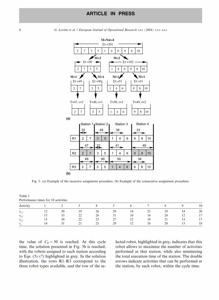
Table 1Performance times for 10 activities

Activity 1 2 3 4 5 6 7 8 9 10

t1,j 12 30 19 26 29 14 21 19 14 20t2,j 15 33 22 26 31 10 14 20 12 17t3,j 15 30 22 23 27 12 19 21 13 17sj 14 31 21 25 29 12 18 20 13 18

2 7 3 10

Στ =201

Στ =99 Στ =102

Στ =49 Στ =50 Στ =51 Στ =51

2 7 3 5 1 4 6 9 8 10

9 8 101 4 63 52 7

M=Nst=4

M=2 M=2

M=1 M=1 M=1 M=1

9 8 10

T=49, r=2

1 4 6

T=50, r=3

3 5

T=48, r=1

2 7

T=47, r=2

5 1 4 6 89

Station 1 Station 2 Station 3

47 22 41 49

9 8 101 4 63 52 7R1

9 8 101 4 63 52 7R2

9 8 101 4 63 52 7R3

30 48 38 33

49 49 50 34

Station 4

(a)

(b)

Fig. 3. (a) Example of the recursive assignment procedure. (b) Example of the consecutive assignment procedure.


ARTICLE IN PRESS

the value of C0 = 50 is reached. At this cycletime, the solution presented in Fig. 3b is reached,with the robots assigned to each station accordingto Eqs. (5)–(7) highlighted in grey. In the solutionillustration, the rows R1–R3 correspond to thethree robot types available, and the row of the se-

lected robot, highlighted in grey, indicates that thisrobot allows to maximize the number of activitiesperformed at that station, while also minimizingthe total execution time of the station. The doublearrows indicate activities that can be performed atthe station, by each robot, within the cycle time.


ARTICLE IN PRESS

2.3.3. Exchange procedure (E)

First we introduce the logical function Wi(q)which returns false if activity i cannot be trans-ferred from station s(i) to station q, and trueotherwise:

W iðqÞ ¼ false if

sðiÞ > q and 9k 2 Y i; sðkÞ > q

or

sðiÞ < q and 9k : i 2 Y k; sðkÞ < q

W iðqÞ ¼ true otherwise:

ð10Þ

Now consider two stations f and q with totalexecution times Tf and Tq (Tf > Tq). If exchangeof activities i (s(i) = f) and j (s(j) = q) is feasible,the new execution times after the exchange are:

T �f ¼ T f trðf Þ;i þ trðf Þ;j ð11Þ

T �q ¼ T q trðqÞ;j þ trðqÞ;i ð12Þ

The exchange is worth-while if:

maxfT �f ; T �qg < T f ð13Þ

From these expressions one can derive the con-dition of exchange:

trðf Þ;j < trðf Þ;i and T q T f < trðqÞ;j trðqÞ;i ð14Þ

The exchange procedure is as follows:

1. Rank all stations in order of total executiontimes.

2. For the most loaded station f and the other sta-tions 1 6 q 6 Nst, q 5 f, in sequence (beginningfrom the least loaded), look for a pair of activ-ities (i,j): s(i) = f, s(j) = q which satisfies theconditions:

W iðqÞ ¼ W jðf Þ ¼ true; ð15Þ

pi;j ¼ pj;i ¼ 0: ð16Þ

3. If these conditions are satisfied as well as condi-tion (14), perform the exchange, recalculateexecution times Tf and Tq and return to step1. If the desired pair of activities does not existfor all possible q, i and j, terminate theprocedure.

2.3.4. Stop condition

The GA stops after performing a pre-definednumber of cycles, NCYC, that is defined as aparameter. At a termination of each cycle, a ‘‘cat-aclysm’’ is performed, i.e. a new population ofsolutions is created, preserving only the best solu-tions. This is the usual procedure in GA to avoidconvergence to local optimum. For each cycle, apre-defined number of crossovers (NCRS) isperformed, unless all solutions converge earlierto a single value of cycle time, without furtherimprovement.

3. Performance evaluation

3.1. Evaluation of the assignment procedures

The assignment procedures were evaluated byconducting tests of the GA with each procedurefor a large set of RALB problems with differentcharacteristics are as follows.

F-ratio––Flexibility ratio, as defined by Dar-El(1973) measures the flexibility of the assembly taskprecedence constraints, by a ratio of the number of0 elements in the precedence matrix (no precedencerequired) to the number of 1 elements in the matrix(hence tasks with no precedence required have anF-ratio of 1). Problems with three levels of F-ratiowere generated and evaluated: low flexibility F-ratio = 0.1, medium flexibility F-ratio = 0.4, andhigh flexibility F-ratio = 0.8.

WEST ratio––work element to station numberratio, as defined by Dar-El (1973) measures theaverage number of activities per station. Thismeasure indicates the expected quality of achieva-ble solutions and the complexity of the problem.Problems with six levels of WEST ratios: 2, 3.33,5, 7.5, 10 and 15 were generated and evaluated.These ratios were achieved by different combina-tions of problems with 20, 100 and 150 activitiesthat were balanced for 10, 20 and 30 stations.

Nr––number of different robot types. Thisparameter affects problem complexity. Two levelswere evaluated, with three and six robot types.

RF––robot (equipment) flexibility, as defined byRubinovitz and Bukchin (1991) measures the num-ber of different robot types that are capable to per-

Consecutive AssignmentRecursive assignment

460.6

564

589

485.5

597

653

440460480500520540560580600620640660

0.1 0.4 0.8F-ratio

Avg. Cycle Time

Fig. 5. Average cycle times vs. F-ratio levels for RETV = 90%.

207.1

150

200

250

Avg. Run Time (sec.)


ARTICLE IN PRESS

form each activity. When RF = 0, each activitycan be performed by a single robot type. WhenRF = 1, each activity can be performed by all ro-bot types. The levels used in evaluation were 0,0.33, 0.66, and 1.

RETV––robot expected time variability, meas-ures the variability in activity performance timesby different robot types. Three levels were tested,0.1, 0.5 and 0.9 for low, medium and highvariability.

The problems generated for this set of parame-ters were solved using each of the two assignmentprocedures with ten replications. The observeddecision variables were the solution cycle time,and the time required to reach a solution. Resultsof the tests for low (0.1) and high (0.9) values ofRETV are summarized in Figs. 4–7.

Analysis of test results shows that, in general,the Consecutive Assignment algorithm achievesbetter solution quality (measured by average cycletime). For all the parameter values tested, the Con-secutive Assignment Procedure results in cycletimes that are shorter or equal to those achievedwith the Recursive Procedure. While solutionquality tends to be similar for both proceduresfor low (0.1) RETV values, it is consistently betterfor high RETV values (both for RETV 0.5 (notshown), and for RETV 0.9) and for lower F-ratio

659

688

631.6

675

688

630.3

600

610

620

630

640

650

660

670

680

690

700

0.10 0.4 0.8 F-ratio

Avg. CycleTime


Fig. 4. Average cycle times vs. F-ratio levels for RETV = 10%.

68.855.8

115 .8

45.435

0

50

100

0.1 0.4 0.8F-ratio


Fig. 6. Average run times vs. F-ratio levels for RETV = 10%.

values. The Recursive Assignment algorithm re-quires shorter run times when RETV values arevery low, however the times required for bothalgorithms are shorter than single-digit numberof minutes. However, for medium and high RETVvalues, and for problems with high F-ratio values,the Consecutive Assignment algorithm solves theproblems in a significantly shorter time. In sum-

405. 2

164 .477.8

2145 .5

49.236.60

500

1000

1500

2000

0.1 0.4 0.8F-ratio

Avg. RunTime (sec.)


Fig. 7. Average run times vs. F-ratio levels for RETV = 90%.

Table 2GA parameter values tested

Parameter Values

IPS 50 80 100NCYC 5 20 50 80NCRS 1500 3000 4500pm 0.5 1 2


ARTICLE IN PRESS

mary, it is always recommended to use the Consec-utive Assignment algorithm to solve the RALBproblem, as the run time required is longer onlyfor a small subset of the problems, and the solu-tion quality is consistently superior.

The results above can be explained further, byanalyzing the differences between the two proce-dures. The Recursive Procedure assigns activitiesto stations using activity times calculated as anaverage of the performance times with different ro-bots. This means that for low time variability be-tween the robots (low RETV values) thisprocedure will be more accurate. This explains itsbetter performance for low RETV values, whichis comparable to the performance of the Consecu-tive Assignment Procedure. Similar performance isalso achieved by both procedures for high F-ratiovalues. This also can be explained by the largersolution space, that allows the approximate Recur-sive Procedure to find good solutions.

3.2. Selecting values for the GA parameters

The performance of a genetic algorithm, andthe quality of solutions, can be affected by the val-ues assigned to the different parameters of thealgorithm. Extensive testing and tuning of theparameter values to be used with the consecutiveassignment procedure of the GA was performed.

Parameters that were evaluated in this set of testsare:

IPS––initial population size (the populationsize may decreases slightly, if equivalent structuresare created during the selection process, in whichcase redundancies are eliminated).

NCYC––number of cycles, i.e. the number oftimes a new set of randomly generated solutionsreplaces the existing set, keeping only the bestsolutions in the population.

NCRS––number of crossovers performed in asingle genetic algorithm cycle.

pm––index of mutation, i.e. a random change byexchanging element positions in a solution string.pm values between 0 and 1 indicate the probabilitythat a newly generated solution string will undergoa single exchange of element positions. Integer pm

values greater than 1 indicate that every newlygenerated solution string will undergo pm ex-changes of element positions.

Different combinations of GA parameter valueswere tested for a representative set of eight RALBproblems with different characteristics. The differ-ent parameter values tested are summarized inTable 2.

The eight different RALB problems were solvedfor all the combinations of the parameter values,with ten replications. The observed decision varia-bles for each of the test runs were a solution cycletime (measure of solution quality), and a computerrun time required (measure of algorithm perform-ance). In selecting the recommended set of GAparameter values, preference was given to solutionquality, as measured by the cycle time, over theperformance, measured by computer run-times.This is due to a fact that most of the problemswere solved within a single-digit number of min-utes (on a personal computer) and there were nomarked differences between them in terms of per-

NCYC=5 NCYC=20 NCYC=50 NCYC=80

Number of Cycles

0

0.05

0.1

0.15

0.2

0.25

0.3

0.35

0.4

Ave

rage

per

cent

of

cycl

e tim

e ab

ove

m

inim

um

Fig. 9. Average percent of cycle time above the minimum cycletime, as function of the number of cycles (NCYC).

NCRS=1500 NCRS=3000 NCRS=4500

Number of Crossovers

0

0.05

0.1

0.15

0.2

0.25

0.3

0.35

0.4

Ave

rage

per

cent

of

cycl

e tim

e ab

ove

m

inim

um

Fig. 10. Average percent of cycle time above the minimumcycle time, as function of the number of crossovers (NCRS).

0.4

0.5

0.6

ycle

tim

e ab

ove

um


ARTICLE IN PRESS

formance times. To establish the recommendedvalues for the GA parameters, the following proce-dure was used:

(1) Each of the eight different RALB problemswas solved with all the 108 possible combina-tions of parameter values, and the combina-tion resulting with the best solution quality(minimal cycle time) was found.

(2) For all other parameter combinations, thepercentage of cycle time above the minimumfound was calculated.

(3) For each combination of the parameter val-ues, the average percentage of cycle timeabove the minimum cycle time value was cal-culated, based on the results of ten replica-tions for the eight different RALB problemssolved.

(4) For each distinct value used for each one ofthe parameters, the average percentage ofcycle time above the minimum cycle timevalue was calculated. This was calculatedbased on an average of cycle time results forall the parameter combinations in which thisparticular parameter value was used.

The results of the average percentage of cycletime above the minimum cycle time, for the differ-ent parameter values tested, are summarized inFigs. 8–11.

It is evident from the test results that there wereno marked differences in quality of solutions for allthe problems, as all solutions were within 0.5 per-cent above the minimum cycle time. However,

0

0.05

0.1

0.15

0.2

0.25

0.3

0.35

0.4

IPS=50 IPS=80 IPS=100

Population Size

Ave

rage

per

cent

of

cycl

e tim

e ab

ove

m

inim

um

Fig. 8. Average percent of cycle time above the minimum cycletime, as function of the initial population size (IPS).

0

0.1

0.2

0.3

Pm=0.5 Pm=1 Pm=2

Probability of Mutation

Ave

rage

per

cent

of

c

min

im

Fig. 11. Average percent of cycle time above the minimumcycle time, as function of the index for mutation (pm).

based on the results, it is possible to recommendthe values of IPS = 100, NCYC = 50, NCRS =3000, and pm = 1 for the GA parameters.


ARTICLE IN PRESS

3.3. Comparison with a branch and bound algorithm

A reduced set of problems, with only three dif-ferent robot types (Nr = 3), was used to comparethe performance of the GA with the consecutiveassignment procedure with the performance ofthe Branch and Bound algorithm for RALB sug-gested by Rubinovitz and Bukchin (1991). Thereis some difficulty in comparing the two algorithms:the GA minimizes the cycle time for a given num-ber of stations, while the B&B algorithm has beendeveloped to minimize the number of stations for agiven cycle time. In order to make a performancecomparison without changing either of the twoalgorithms, a set of problems with different prob-lem parameters was generated, and a special com-parison procedure was used. The problemcharacteristics used to generate this set of prob-lems are summarized in Table 3. This experimentaldesign consists of a total of 108 problems, for allthe combinations of the parameters set. The com-parison procedure was as follows:

• The GA with the consecutive assignment proce-dure was used to solve the entire set ofproblems, with ten replications (10 differentproblems were generated for each combinationof the parameters set). An average cycle timefor each parameter combination, resulting fromthe 10 replications, was calculated.

• The B&B algorithm was solved for the same setof problems, attempting to minimize the num-ber of stations for the average cycle timeachieved by the GA.

• A comparison was made between the number ofstations used for the GA and the number of sta-tions found by the B&B algorithm, for the sameproblems.

Table 3Characteristics of the problem set

Parameter Values

F-ratio 0.1 0.4 0.8WEST ratio 2 5 10Nr 3RF 0 0.33 0.66 1RETV 0.1 0.5 0.9

B&B could solve only a small subset of 24 prob-lems, of all the problems generated, to optimality.For this subset, equal quality solutions wereachieved for 23 of the problems by both algo-rithms, and the B&B solution was better for onlyone problem. For all the other problems, the heu-ristic version of B&B had to be used. Both algo-rithms gave solutions of equal quality for about30% of the problems. For the other problems thesolutions achieved by the GA were of higher qual-ity, balancing the line with one or two less stations.This superiority of solutions of the GA was dem-onstrated in particular for problems with greatercomplexity (high values of F-ratio and WEST-ratio). An important advantage of the GA is thatthe time required to reach a solution is not grow-ing with problem complexity, and is dependenton the set of parameters of the GA (initial popula-tion size, number of cycles and number of crosso-vers). Most solutions were achieved in few seconds(none exceeded a single-digit number of minutes)on a Pentium3 personal computer.

3.4. Consistency and robustness of the Genetic

Algorithm

In order to check the consistency and robust-ness of the GA, five representative problems withvery different problem characteristics were se-lected. Each problem was solved by the GA tentimes, using different problem parameters (suchas initial population size), and randomly generat-ing different initial populations. At selected inter-vals in the solution process (after a givennumber, x, of crossovers), the best solution valueswere recorded. The purpose was to show that thedifferent solutions of a problem converge to a com-mon value of the solution�s quality. The basic ideabehind this test was that if we can show conver-gence to similar solution quality, even whenchanging parameters such as the initial populationsize, then we can conclude that this is not a ran-dom event, and the algorithm is consistent and ro-bust. This was measured at each interval bycalculating the coefficient of variance between thebest solution values of the 10 GA runs. In threeof the five problems tested, the algorithm con-verged to solutions of equal quality (coefficient of

0

0.1

0.2

0.3

0.4

0.5

0.6

0.7

0.8

0.9

0 5000 10000 15000 20000 25000

NCRS - Number of Crossovers

Coe

ffic

ient

of

vari

ance

WEST-ratio = 5, F-ratio = 0.8, RETV= 50%

Fig. 12. Coefficient of variance between the best solutions of 10different algorithm runs as function of number of crossovers(NCRS).


ARTICLE IN PRESS

variance equal zero). In the two other problems ofhigher complexity (high F-ratio and WEST-ratio values) the algorithm converged to coeffi-cients of variance of 0.11% and 0.31%, respectively.The convergence graph for the last problem testedis shown in Fig. 12. This graph shows that afterabout 20,000 crossovers, different parameters usedfor the GA all yield solutions of very similar quality(Coefficient of variance of less than 0.31%).

4. Conclusion

The objective of this work was to develop anefficient solution for the robotic assembly line bal-ancing (RALB) problem. This solution aims toachieve a balanced distribution of work betweendifferent stations (balance the line) while assigningto each station the robot best fit for the activitiesassigned to it. The result of such solution wouldbe an increased production rate of the line (byachieving a minimal cycle time).

Two different procedures for adapting the GAto the RALB problem and assigning robots to sta-tions are introduced: a recursive and a consecutiveprocedure. Local exchange procedure is used tofurther improve the quality of solutions. The bestcombination of these procedures and GA parame-ters is reached by testing on an extensive set of ran-domly generated problems. The GA developed isshown to be consistent and robust. It achievessolutions of higher quality than a Branch and

Bound algorithm, and solves large and complexproblems very efficiently.

References

Alander, J., 1995. An indexed bibliography of genetic algo-rithms in manufacturing. In: Lance, C. (Ed.), PracticalHandbook of Genetic Algorithms New Frontiers, vol. II.CRC Press, Boca Raton, FL.

Bukchin, J., Tzur, M., 2000. Design of flexible assembly line tominimize equipment cost. IIE Transactions 32, 585–598.

Dar-El (Mansoor), E.M., 1973. MALB––a heuristic techniquefor balancing large single-model assembly lines. AIIETransactions 54, 343–356.

Everitt, B.S., 1974. Cluster Analysis, first ed. John Wiley &Sons, New York.

Falkenauer, E., 1998. Genetic Algorithms and GroupingProblems. John Wiley & Sons Inc.

Goldberg, D., 1989. Genetic Algorithms in Search, Optimiza-tion and Machine Learning. Addison Wesley, Reading, MA.

Graves, S.C., Holmes, C.R., 1988. Equipment selection andtask assignment for multiproduct assembly system design.The International Journal of Flexible Manufacturing Sys-tems 1, 31–50.

Kim, H., Park, S., 1995. Strong cutting plane algorithm for therobotic assembly line balancing problem. InternationalJournal of Production Research 33 (8), 2311–2323.

Kim, Y.K., Kim, Y.J., Kim, Y., 1996. Genetic algorithms forassembly line balancing with various objectives. Computersand Industrial Engineering 30 (3), 397–409.

Kim, Y.K., Kim, Y., Kim, Y.J., 2000. Two-sided assembly linebalancing: a genetic algorithm approach. Production Plan-ning and Control 11 (1), 44–53.

Khouja, M., Booth, D.E., Suh, M., Mahaney Jr., J.K., 2000.Statistical procedures for task assignment and robot selec-tion in assembly cells. International Journal of ComputerIntegrated Manufacturing 13 (2), 95–106.

Mahalanobis, P.C., 1936. On the Generalized Distance inStatistics. National Institute of Science in India 12, 49–55.

Gen, M., Tsujimura, Y., Li, Y., 1996. Fuzzy assembly linebalancing using genetic algorithms. Computers and Indus-trial Engineering 31 (4), 631–634.

Nicosia, G., Paccarelli, D., Pacifici, A., 2002. Optimallybalancing assembly lines with different workstations. Dis-crete Applied Mathematics 118, 99–113.

Owen, A.E., 1985. Assembly with Robots. Kogan Page Ltd.Ponnambalam, S.G., Aravindan, P., Naidu, G.M., 2000. A

multi-objective genetic algorithm for solving assembly linebalancing problem. International Journal of AdvancedManufacturing Technology 16, 341–352.

Rubinovitz, J., Bukchin, J., 1991. Design and balancing ofrobotic assembly lines. In: Proceedings of the Fourth WorldConference on Robotics Research, Pittsburgh, PA.

Rubinovitz, J., Bukchin, J., Lenz, E., 1993. RALB––a heuristicalgorithm for design and balancing of robotic assemblylines. CIRP Annals 42 (1), 497–500.


ARTICLE IN PRESS

Rubinovitz, J., Levitin, G., 1995. Genetic algorithm forassembly line balancing. International Journal of Produc-tion Economics 41, 343–354.

Sabuncuoglu, I., Erel, E., Tanyer, M., 2000. Assembly linebalancing using genetic algorithms. Journal of IntelligentManufacturing 11, 295–310.

Starkweather, T., McDaniel, S., Mathias, K., Whitley, D.,Whitley, C., 1991. A comparison of genetic sequencingoperators. In: Proceedings of the Fourth Interna-

tional Conference of Genetic Algorithms and theirApplications.

Suresh, G., Vinod, V.V., Sahu, S., 1996. A genetic algorithm forassembly line balancing. Production Planning and Control 7(1), 38–46.

Whitley, D., 1989. The GENITOR algorithm and selectivepressure: why rank-based allocation of reproductive trials isbest. In: Proceedings of the Third International Conferenceon Genetic Algorithms and their Applications.

Documents

A genetic algorithm for robotic assembly line balancing · A genetic algorithm for robotic assembly line balancing Gregory Levitin a,*, Jacob Rubinovitz b, Boris Shnits b a DivisionofPlanning,DevelopmentandTechnology