A generative model for age and income distribution

Ozhamaratli et al.

RESEARCH

A generative model for age and incomedistributionFatih Ozhamaratli1*, Oleg Kitov2 and Paolo Barucca1

*Correspondence:

[email protected] College London, Gower

Street, WC1E 6BT London, UK

Full list of author information is

available at the end of the article

Abstract

Each individual in society experiences an evolution of their income during theirlifetime. Macroscopically, this dynamics creates a statistical relationship betweenage and income for each society. In this study, we investigate income distributionand its relationship with age and identify a stable joint distribution function forage and income within the United Kingdom and the United States. Wedemonstrate a flexible calibration methodology using panel and populationsurveys and capture the characteristic differences between the UK and the USpopulations. The model here presented can be utilised for forecasting income andplanning pensions.

Keywords: Income Dynamics; Agent Based Model; Pension System

1 IntroductionA universal element of societies is the emergence of hierarchical organisation struc-

tures within professions. People develop work experience through time and manage

to obtain jobs of increasing responsibility and increasing level of income with time.

Hence, it is a natural property of income distribution to be correlated with work

experience and age; nevertheless, most income models do not study the relationship

between income and age, and consequently between income distribution and demo-

graphic changes. This paper introduces a model of income, dependent on age-specific

model parameters and random shocks. The model contributes to the understanding

of the relationship between age and income and its dynamics.

Our aim is to compare the estimated parameters in the UK and the US age and in-

come distribution to find out similar characteristics of age and income across states,

as well as the contrasting differences. A simple age and income model is fundamen-

tal for the development of a sustainable pension system. The model focuses on the

age and income relationship and further factors, such as occupational levels, are not

considered. The model is estimated via panel survey data from the UK and popula-

tion surveys from the USA. The data from panel surveys track the same individuals

for the duration of the survey, and the population survey is repeated with different

people each wave. The results reflect a clear income-age relationship in the UK and

US, a clear structure of the joint distribution characterised by rapidly increasing

income at younger ages, followed by income levels stabilising near mean income

but spreading till retirement. At this point, the income decreases and concentrates

around mean retirement income. The paper demonstrates a flexible methodology to

estimate parameters from population surveys, as well as panel surveys. The paper

provides a simple generative model to evolve age-income population for simulation

arX

iv:2

108.

0084

8v1

[ec

on.G

N]

26

Jul 2

021

mailto:[email protected]

Ozhamaratli et al. Page 2 of 29

and forecasting purposes, which can constitute the foundation for future studies of

financially sustainable pension systems by providing a benchmark for capturing age

and income relationship. The purpose is to have a baseline model simple enough for

isolating age and income relationship of income dynamics. Such a model will serve

for investigating the properties of a sustainable and balanced pension system. The

mean and standard deviation statistics from the panel and population surveys on

Fig. 6, Fig. 7, Fig.2 from observed panel data and simulation results reflect a clear

relationship between age and income. More complex models, which investigate ad-

ditional factors, and profile heterogeneity of income dynamics are out of the scope

of our work.

Previous research on income have been conducted, and the research focused on

investigating and explaining wage dynamics. Champernowne explicitly introduces

a first-order Markov process to model the time-evolution of wages[1]. Following

Markov process path, the validity of the first-order Markov assumption is tested

by Shorrocks[2]. Following research introduces a second-order Markov process, yet

neither of these works links individual wage dynamics to time-evolution of the dis-

tribution of wages [3]. A different approach focused on poverty, which deals with

modelling individual data using linear regression and transitioning to poverty (pro-

bit model)[4]. A more comprehensive model incorporating various factors is devel-

oped to estimate transition probability in wage quintiles conditioned on various

regressors, including education, experience and age [5], and study both intra- and

inter-group inequality. The persistence of the low pay state and on factors affect-

ing the low pay probability in a generalized regression model is expressed. For

modelling low income transitions the previous research use British Panel Data for

the ′90s, focus on the transition probability and state dependence for the poverty

status[6]. They define poverty transition equation, a coarse-grained dynamics. Fo-

cus on inequality and upward mobility between quintiles considering gender effects

are investigated [7]. The previous models in literature either incorporate numerous

external variables, distribution characteristics and functions, such as innovation

constants or limiting their scope to the investigation of dependence on a single vari-

able[8][9]. A more recent article by Guvenen investigated a model for which focal

variables are the human capital consisting of education, work experience, and id-

iosyncratic shocks [10], following research modelled male income for studying the

impact of labour income taxation policy on inequality [11] The referred life-cycle

model’s distribution characteristics of the pre-tax income arise from the differences

in the individual’s ability to learn new things and idiosyncratic shocks. Previous

research tried to capture the income dynamics with Markov Models, linear autore-

gressive models, or by relying on econometric toolset such as covariance matrices.

We investigate a generative model with an empirical distribution for sustainable age

and income relationship in a population; we achieve this via an income evolution

model with an age-dependent parameter, estimated from previous population and

panel surveys.

In contrast to previous research, our study introduces a dynamic model that

describes the income-dependent only on age and previous income. This paper in-

vestigates the stationary property of the income distribution dependent on age. We


provide a model in which the mean and variance of income given age are preserved

at any time point.

2 MethodsWe introduce a simple model which focuses on age and income relationship and dif-

fers from recent literature by not incorporating other variables such as occupational

level, level of education and skill coefficients. The model is stationary, i.e. the mean

and variance of income given age are preserved in time. The model is utilised to rep-

resent observed panel data for gaining empirical insights regarding age dependant,

income dynamics and mobility. The calibrated model can be utilised as a simple

generative model to evolve an age-income population for simulation purposes and

it provides a theoretical background for studies focusing on ageing and pension in-

come of the population. We initially assume the following model, by which µ(.) and

σ(.) represent a function of age, income, and individual-specific additional param-

eters θi or λi, for the sake of generality. µ(.) is a function capturing mean income

characteristics, and σ(.) captures the variational characteristics of the income. We

consider the following individual income stochastic process for an economic agent i

characterised at each time step t by a given age ai and income yi:

yi(t+1) = µ(ai(t+1), yit|θi) + σ(ai(t+1), yit|λi)ηit (1)

The characterising insights on Fig.2 from the panel data lead to the assumption

that the probabilistic step at time t depends only on the age and income of the

preceding step.

2.1 Defining Income and Age Dynamics

Earnings of individual i at the time step t is denoted as Yi,t and its logarithm is

yi,t. The parameters that describe the income process are: age-dependent persis-

tence parameter qa, age-dependent mean µa and age-dependent standard deviation

σa. The income shock process consists of independent random shock ηit which is

normally distributed with mean zero and variance 1, and it is applied to σa, the

model can be defined as follows:

yia+1,t+1 = qayia,t + µa + σaη

it (2)

Averaging income y, for individuals who are a years old, gives ya ,which denotes

the average income for age group a across all individuals i and periods t. Assuming

that the age-dependent income profiles are stationary, we can average incomes yia,tacross individuals and time to get the following equation:

ya+1 = qaya + µa (3)

where ya denotes the average income for age group a, taken across all individuals i

and periods t. The following equation can find the estimator for µa:

µa = ya+1 − qaya (4)


The income data from different waves are inflation adjusted to isolate effects of

economic growth.

2.2 Data

The British Household Panel Survey (BHPS)[12] from the UK and The Current

Population Survey (IPUMS CPS)[13] from the USA are used for estimating the

model parameters of the model (2) and comparing the results of simulated data and

surveys. The BHPS is a Panel Survey conducted between 1991-2008. For our model

we focus on labour income data, which captures wage, salary or self-employment

income. To investigate population characteristics, we also incorporate other income

sources and call it ”Total Income”, which additionally captures the transfers, pen-

sions, grants, aids, state-benefits, dividends, capital income and rents. BHPS pro-

vides individuals specific longitudinal weights for ensuring the representativeness of

the population. Two types of weights are provided with BHPS. The first wave is

weighted for adjusting population marginals at the households and post-stratified

to the population age by sex marginals. Consecutive waves are re-weighted to take

into account sample attrition, variables such as address change, household region,

age, sex, race, employment status, income total and composition, educational quali-

fications[14]. Panel Survey is conducted via questionnaires with tracked individuals

of the initial sample. There is an extension to the sample population in 1999.

For the USA, IPUMS CPS is used, which is annually conducted with different

samples each year. In contrast with BHPS, the Labour Income does not include

self-employed income, and the weights are cross-sectional. Income distribution, age

distribution and income-dependent age distribution from the surveys are utilised for

parameter estimation and further analysis. qa, µa, σa are the key parameters esti-

mated according to the proposed model. Following investigation and interpretation

of the estimated parameters, these parameters are used to simulate the population’s

income transitions. The simulation is initialised using the panel data from the wave

1, and the income evolution function 2 of the model is applied transitively in an

iterative approach to the data for simulating successive waves. The simulated data

is plotted, interpreted and finally compared with the observed data.

Fig. 1 reflects the Population Pyramid in the UK and USA, and how the shape

evolved over the 18 years considered. The UK population sample from BHPS has

a relatively balanced population with a slight weight towards younger cohorts ini-

tially in 1991, which denotes Wave 1. The UK population gradually got older, and

the population pyramid reflects mass’s shift towards older generations, this shift

happened gradually over the years. The US population from CPS reflects a young

population in Wave 1 with a notable skew towards younger cohorts, after 17 years

the US population loses this property towards younger cohorts and gets signifi-

cantly older. Both the UK and US population get older and reflect a trend towards

an ageing population, which will significantly impact the pension system.

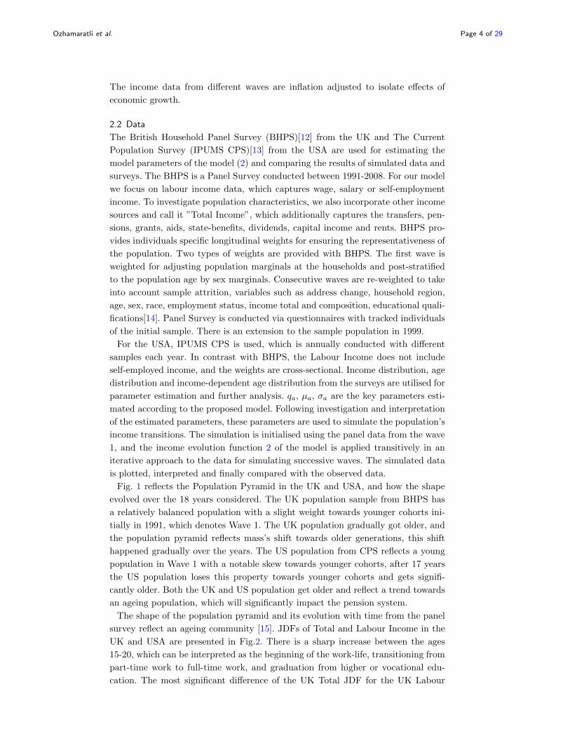
The shape of the population pyramid and its evolution with time from the panel

survey reflect an ageing community [15]. JDFs of Total and Labour Income in the

UK and USA are presented in Fig.2. There is a sharp increase between the ages

15-20, which can be interpreted as the beginning of the work-life, transitioning from

part-time work to full-time work, and graduation from higher or vocational edu-

cation. The most significant difference of the UK Total JDF for the UK Labour


(a) UK Pyramid Wave 1

(b) UK Pyramid Wave 18

(c) USA Pyramid Wave 1

(d) USA Pyramid Wave 18

Figure 1: Population Pyramid for the UK & USA Income between Ages 15-100


(a) UK Labour JDF (b) UK Total JDF

(c) USA Labour JDF (d) USA Total JDF

Figure 2: All Waves JDF for UK and USA Income between Ages 15-100

JDF is the tail section corresponding to the retired population, which denotes the

significant percentage of individuals older than 55. The tail section is relatively con-

centrated, which can be explained by the state pension benefit levels and mandatory

social security system. The US population reflects a surprisingly sparse older cohort

for the Total Income data, and the most significant difference to the UK is the rel-

atively lower income levels compared to the wage income. A higher variance spread

to a wider band, which might be caused by a non-standard retirement system not

supported by strong state pension benefit and mandatory pension schemes during

employment.

The comparison for the model simulation and observed data shows common char-

acteristics, as the joint distribution of age and income in logarithmic scale is pre-

sented in Fig.2 : an initial sharp rise between the entrance to the graph on 16 years

old, the amount of 16 years old includes pocket money, allowance and part-time or

internship jobs. There is a steep increase in mean and variance between the initial

income and income at the age of 20. The increase is sharper for the mean in com-

parison to the variance. The population’s mass has similar characteristics with near

23k GBP annual income, and for ages between 20-45. Between ages 65-75, there is a

significant decrease in income and after 75, the income converges to a certain mean.

The data and the models provide an essential tool to tackle problems related to an

ageing population and shocks introduced by technological and political changes.

In the following sections we will focus on Labour Income and employed labour

population. Total Income covers all of the income streams including Transfer In-


come such as pocket-money, Labour Income, Capital Income, and Pension Income;

these different streams might be governed by varying dynamics non-uniform across

the type of income; so we decided to focus on Labour Income, which involves the

broadest section of the population; with most significant impact. The only other

primary source of income in terms of gross value is the Capital Income, which might

be significantly affected by other factors such as inter-generational shifts, market

conditions and global financial state. In order to focus on labour income dynamics,

the other income sources are left out of our modeling.

3 Data Processing and CalibrationBHPS provides a vast amount of socio-economical data for each individual and

household participating in the study. The columns of income, age data, the individ-

ual’s statistical weight -representative of the British population and overall survey-

with the individual’s intra-wave unique identifier mostly suffice for this paper’s

scope. PID, Wxage12, wFIYR, Wxrwght fields of BHPS are used for each wave.

The Income variable xfiyr is each individual’s annual income, including labour

income, benefits, pensions, transfer income, and investment income. Participants

were asked according to annual income in the reference year from September in

the year prior to the interview until September in which interviewing begins [14].

The income figures are adjusted for inflation, as part of pre-processing. During the

dataset preparation, a floor wage is determined to exclude in labour income, which

denotes to excluding part-time and short-employment income. The income data is

inflation-adjusted and transformed into log-domain.

IPUMS harmonizes the CPS and provides IPSUM CPS micro-data. The IPSUM

CPS includes a large spectrum of topics such as demographics and employment,

as well as supplemental studies such as the Annual Social and Economic Supple-

ment (ASEC). Each individual can be identified by ”CPSIDP”, ”INCTOT” and

”INCWAGE” correspond to the total income and wage income, and ”ASECWT”

denotes the weights derived from ASEC Supplement. The data set is topcoded, and

specific codes are used for labelling missing and incorrect data. The ages over 80, 90

and 99 are top-coded till 2004, and after 2004, the top-coding bins are determined

as 80,85,90 and 99 by the panel data collectors[13]. Although this dataset contains

high-income individuals, there is top-coding applied, so individuals with very high

income are not included.

3.1 Fitting Distributions

Estimating the income evolution function parameters is the most critical part of the

research, and the decision depends on various factors such as the type of data, bias,

and assumptions. Various techniques are investigated, leading to different results,

with each having unique strengths and weaknesses.

The first method investigated is Generalized Method of Moments (GMM), which

presumes that the first three moments of the income evolution functions provide

the necessary information for approximating the underlying generative process. The

equations of the first three moments of the income evolution equation can be solved

for the parameters qa, σa, µa. Both of the BHPS from the UK and the IPUMS CPS

from the USA can be used for estimation with Generalized Method of Moments


(GMM) with first three moments.

The second method utilises the micro-data from the longitudinal surveys, which

tracks the individual for consecutive years. The parameters are approximated to fit

the income evolution function using least squares minimisation for the individuals

participating in the studies for consecutive years. The BHPS from the UK is a

suitable micro-data consisting of a panel survey, and the survey tracks income of

the same individuals over the years.

3.2 Estimation for Generalized Method of Moments (GMM)

The three moments of the age income evolution function are utilised to find a

polynomial; afterwards, the equation is solved for qa, σa and µa; at this point, a

observed solution for parameters is found, but the relationship captures only the

dynamics of the first three moments. Calculations can be found in appendices. The

statistical variables such as ya are found for each wave and than averaged across

waves for finding a one set of stationary variables, which can be used to estimate

qa, σa, µa. The details and derivations for the GMM estimation technique can be

found in appendix.

3.3 Estimation of Least Squares for Micro Data

The Least Square Method requires that an individual’s income for two consecutive

years be existent in the dataset, this restriction is fulfilled by the BHPS, a panel

survey, but the CPS IPUMS population survey does not satisfy this condition. The

income data from two consecutive years per agent is used to estimate age-specific

parameters, which characterise the income evolution function at Eq.2. LSM tries to

estimate parameters by fitting the data to the income evolution function.

4 The generative modelThe model can also be used for simulation and forecast, tracking income trajectories

of the individuals, providing a bench table for observing the stylized facts and

complex properties of the income dynamics. Following the estimation of model

parameters, the model is bootstrapped with data from wave 1 for initialising the

simulation. Each individual from wave 1 is initialised as an agent in our model.

According to Age Income Evolution Dynamics Eq. 2 , the income of these agents is

transitively updated at each consecutive wave update. ηit provides the random feed,

which introduces variability for the income evolution of the agents. At each wave

update, a new generation of agents consisting of 25 years old agents from the initial

wave is injected. Following each wave, distributions corresponding to the state of

the simulated population are calculated. A full calibration of the model is shown in

the Supplementary Material.

5 ParametersThe optimized performance of these three methods are compared and discussed in

the following sections.

No boundaries are explicitly imposed by LSM estimation.

The µ, σ and q variables are independent of each other, but the estimation process

or data itself can introduce a slight dependence. The GMM estimation technique


(a) qa with GMM (b) σa with GMM

(c) µa with GMM

(d) qa with LSM (e) σa with LSM

(f) µa with LSM

Figure 3: qa, σa and µa Plots for UK Labour Income


results in minimal q values near 0, so the estimated parameters approximately

resemble an auto-regressive model. However, despite near 0 negligible q values, the

q plot has a distinct shape with an increasing trend with a small decrease between 25

and 30, has very different characteristics depending on the estimation method. The

GMM estimation method results in minimal q and the µ reflects the characteristics

of y, which is in compliance with this estimation method’s nature. The µ value

increases at first and then plateaus and slightly decreases near retirement. On the

contrary LSM estimation mainly characterises the income with an increasing q

parameter, so the µ parameter has limited effect and reflects a decreasing trend.

σ values reflect a distinct trend of initially decreasing values with a spike around

the age of 34 followed by a stable decrease and noisy plateau with a minor increase

towards 55. The LSM with bootstrap is the most accurate estimation method and

reflects the characteristics of the model clearly.

GMM

GMM estimation technique approximates the µa values to be consistently around

10 and the qa values are around 0 with an initial sine-like wave followed by a steady

increase. The σa values are around 0.8 and have a positive trend. qa values dis-

play a positive trend as well. The ya and std(y)a plots of the simulation is similar

to the observed data, but the standard deviation plot is particularly noisy. The

JDF of the simulation on Fig. 10 is sparse, consistent; but not highly concentrated

around mean. Both of these methods depends on assumptions about the dynamics

of the income evolution function. The GMM method assumes that the first three

moments of the equation are enough for estimating the parameters because they

provide a solvable system. However individual characteristics in an age group such

as different income levels and clusters within are lost during the moment estimation.

LSM by individual transitions

To use LSM to approximate the parameters, one needs the individual income tran-

sitions in consecutive years, thus identifying the same individual in consecutive

cohorts is necessary, the panel studies such as BHPS satisfy this condition. The

age-dependent income evolution function is fitted with individual income transi-

tions of consecutive years. The JDF of simulation has concentrated heat regions

around the mean, and the trend is decreasing unlike the observed data. Imposing

boundaries to the parameter space results in better parameters, which results in

consistent parameter plots and the ya plot of the simulation reflect similar shape

with the observed data Fig. 6 and Fig. 7. The JDF of the simulation on Fig.11 is

able to reflect the dispersion among various clusters better because unlike the other

methods heavily depending on the statistics such as mean and standard deviation

of the entire age group, the LSM utilises individual-level microdata.

The 95% confidence interval with 2000 bootstrap samples for the estimated pa-

rameters from UK microdata by LSM can be found on Fig. 5

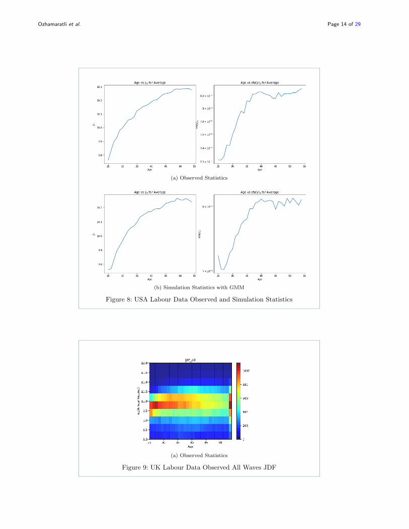
It is evident from the plots of ya and std(ya) for the observed and simulated

data that the model can capture the characteristics of the income conditional on

age distribution, and the characteristic stationary property of this model can be

observed on Fig. 6 and Fig. 7.


(a) qa with GMM (b) σa with GMM

(c) µa with GMM

Figure 4: qa, σa and µa Plots for USA Labour Income

(a) qa with LSM (b) σa with LSM

(c) µa with LSM

Figure 5: qa, σa and µa Confidence Interval for UK Data LSM Estimation


A close investigation of Fig. 6 and Fig. 7 on UK Labour Income Data suggests

that the GMM is most successful for reflecting the outcomes with similar mean and

standard deviation characteristics of all waves after simulation with 18 waves that

were simulated with the parameters qa, σa, µaestimated by the GMM. But LSM

reflects the individual trajectories, and JDF more accurately.

(a) Observed Statistics

Figure 6: UK Labour Data Observed Statistics

The results showing the performance of GMM method is in Fig.8.

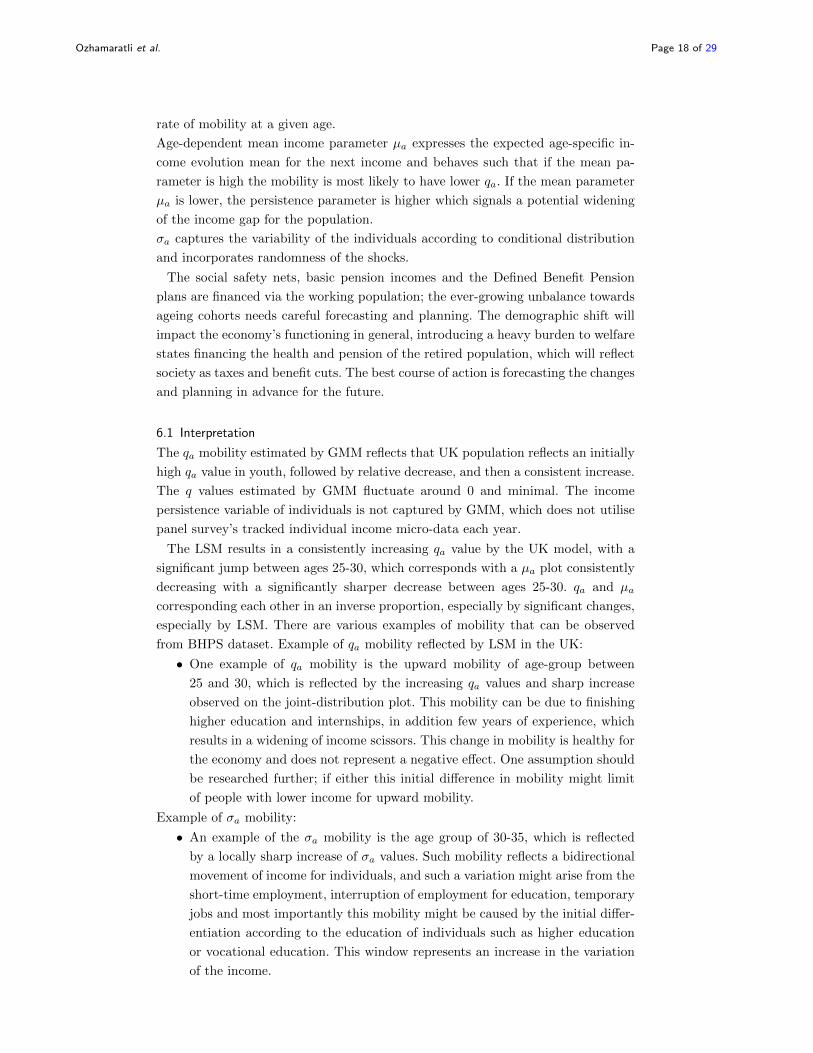
A general analysis of the comparison of joint distribution of age and inflation-

adjusted income results in the following plots for weighted observed data and sim-

ulated data in Fig.9 and Fig.10:

JDF of the simulated UK Labour data is in parallel with the expectations for

GMM Estimation method, consistent and stable, resembling a similar shape but

not concentrated for the heat regions with intense concentrations on Fig. 6 and Fig.

7.

The main differences between the observed and simulated JDFs are concentration

of the mass of the population between 23 and 50.

5.1 Wave-Specific analysis

The population from wave-1 is used for bootstrapping the simulation and the

weights of the individuals are not incorporated to the simulation, because the income

evolution Func.(eq. 2) is the focus of this paper, and the main purpose is not the

perfect representativeness of the initial wave. The new agent injection on 1999

by panel survey is reason of difference in the UK simulation and observed JDF

plots. Although the simulation’s initial state is bootstrapped as the unweighted

dataset, starting from the second wave, the JDF of the simulated population(Fig.

11) resembles the characteristics of the JDF from the panel survey with the weighted

population, which reflects that the model is successfully capturing income evolution

dynamics.


(a) Simulation Statistics with GMM Estimation

(b) Simulation Statistics with LSM Estimation

Figure 7: UK Labour Data Simulation Statistics



(b) Simulation Statistics with GMM

Figure 8: USA Labour Data Observed and Simulation Statistics


Figure 9: UK Labour Data Observed All Waves JDF


(a) Simulation Statistics with GMM Estima-tion

(b) Simulation Statistics with LSM

Figure 10: UK Labour Data Simulation All Waves JDF


(a) 1992 Observed Data (b) 1995 Observed Data

(c) 2005 Observed Data

(d) 1992 with GMM Estimation (e) 1995 with GMM Estimation

(f) 2005 with GMM Estimation

(g) 1992 with LSM Estimation (h) 1995 with LSM Estimation

(i) 2005 with LSM Estimation

Figure 11: JDF Plots of Simulation for UK Labour Income


5.2 A Simple Pension System

A financially sustainable pension system can be characterised by the balance be-

tween inflow and outflow of funds. The specifics and stability of pension system is

out of the scope of this paper, and needs case specific detailed modelling. For a gen-

eral demonstration, we assume simple inflow and outflow dynamics(Eq.5 and Eq.6),

which are derived to represent statistical properties of the savings and consump-

tion. Figure 12 reflects the imbalance between inflow and outflow, which results in

a deficit.

Pension is assumed to be annually £16368, in light of the median net income before

housing costs for all pensioners from DWP Pensioners Income Series in 2008/2009

[16]. Constant alpha for pension saving rate is selected to be 0.0775 to 0.2, in light

of OECD Pension Report statistics [17].

Outflow Ot in a given year t is characterised by constant annual pension amount

p, and count of people above 65 ca>65 is assumed to be pensioner counts.

Ot = pca>65 (5)

Inflow It in a given year t is characterised by constant pension contribution rate α

and total labour income of individuals ya

It = α∑i

(ya≤65) (6)

The amounts are adjusted for inflation and reflect the 2009 levels. The inflow and

outflow plots on Fig. 12 from our simplified generalisation of the pension system

reflect a deficit.

(a) Inflow & Outflow

Figure 12: UK Inflow Outflow Plot of our Simple Pension System

6 DiscussionThe income evolution eq. 2 of the proposed model consists of the parameters qa,

µa, σa: the persistence coefficient for the respective age group qa, determines the


rate of mobility at a given age.

Age-dependent mean income parameter µa expresses the expected age-specific in-

come evolution mean for the next income and behaves such that if the mean pa-

rameter is high the mobility is most likely to have lower qa. If the mean parameter

µa is lower, the persistence parameter is higher which signals a potential widening

of the income gap for the population.

σa captures the variability of the individuals according to conditional distribution

and incorporates randomness of the shocks.

The social safety nets, basic pension incomes and the Defined Benefit Pension

plans are financed via the working population; the ever-growing unbalance towards

ageing cohorts needs careful forecasting and planning. The demographic shift will

impact the economy’s functioning in general, introducing a heavy burden to welfare

states financing the health and pension of the retired population, which will reflect

society as taxes and benefit cuts. The best course of action is forecasting the changes

and planning in advance for the future.

6.1 Interpretation

The qa mobility estimated by GMM reflects that UK population reflects an initially

high qa value in youth, followed by relative decrease, and then a consistent increase.

The q values estimated by GMM fluctuate around 0 and minimal. The income

persistence variable of individuals is not captured by GMM, which does not utilise

panel survey’s tracked individual income micro-data each year.

The LSM results in a consistently increasing qa value by the UK model, with a

significant jump between ages 25-30, which corresponds with a µa plot consistently

decreasing with a significantly sharper decrease between ages 25-30. qa and µa

corresponding each other in an inverse proportion, especially by significant changes,

especially by LSM. There are various examples of mobility that can be observed

from BHPS dataset. Example of qa mobility reflected by LSM in the UK:

• One example of qa mobility is the upward mobility of age-group between

25 and 30, which is reflected by the increasing qa values and sharp increase

observed on the joint-distribution plot. This mobility can be due to finishing

higher education and internships, in addition few years of experience, which

results in a widening of income scissors. This change in mobility is healthy for

the economy and does not represent a negative effect. One assumption should

be researched further; if either this initial difference in mobility might limit

of people with lower income for upward mobility.

Example of σa mobility:

• An example of the σa mobility is the age group of 30-35, which is reflected

by a locally sharp increase of σa values. Such mobility reflects a bidirectional

movement of income for individuals, and such a variation might arise from the

short-time employment, interruption of employment for education, temporary

jobs and most importantly this mobility might be caused by the initial differ-

entiation according to the education of individuals such as higher education

or vocational education. This window represents an increase in the variation

of the income.


In general, the shape of the distribution can be explained in three periods; the

first period is the introduction to employment and teenagers, which represents in-

come from part-time and temporary jobs at the beginning and start of full-time

employment it sharply increases on Fig.2.

The age group of 25-55 denotes the main productive era of the economic life,

and the income reflects a high dispersion. All of the factors and random shocks act

together and result in dispersed but a consistent distribution. Mobility wise this

era provides opportunities for upward mobility and possesses downward mobility

risks. At the end of this period, income tends to decrease slightly, which reflects a

decrease in productivity. Another limiting factor is the minimum wage and state

benefits, which introduces a lower bound envelope for the mass. Income sources and

affecting factors of individuals in this era vary greatly, which results in the widest

dispersion in the entire life-span. Some of the factors are education, social strata,

adaptability to innovation, total-work hours per week, experience and expertness,

seniority of the jobs and ageism. The third and final era represents the exit from

the workforce and retirement, and temporary or part-time jobs for low-income old

individuals. The income decreases gradually as the number of individuals exiting

workforce increases with time, the income stabilises, and variation decreases sig-

nificantly. Income in this era is relatively low, and the source is usually pension

benefits, state support or temporary jobs. This model’s outcomes can be used for

various purposes; the most apparent fields for drawing consequences and planning

are the works on inequality and mobility depending on age. Characteristics of work-

force entrance, work-efficiency of individuals per age, the structure of the society,

pension system, income stability, and the taxation system are the most obvious

fields.

In the paper, two main estimation techniques are investigated, and the correspond-

ing results from the simulated waves are presented. The first estimation method

investigated is GMM Estimation. The income regions appear smoothed and spread.

The second estimation method investigated is LSM, it utilises the microdata and is

suitable for capturing an agent’s income evolution. The JDFs from the simulated

waves have the most similar mean characteristics to the observed data.

The LSM evidently performs better by utilizing longitudinal microdata; the GMM

estimation method can be applied to both population and panel surveys, provides

feasible distributions but with unrealistic modeling of an agent’s individual income

trajectory.

6.2 Conclusions

We demonstrated (1) a clear income-age relationship, which is reflected by the data

from BHPS and IPSUM CPS, as well as simulations. (2) a clear structure of the

joint age-income distribution in both the UK and USA. (3) a flexible methodology

to estimate parameters from population surveys, as well as panel surveys. (4) a

simple generative model to evolve the age-income population with real constraints

for evaluating general policy scenarios, that is agnostic about occupation levels.

The model can be interpreted as delivering a premise that the information of an

individual’s experience and education can be encapsulated by income. Although in

early career, the income dynamics are governed by the initial difference at the level of


education and profession; the main dynamics governing income transitioning can be

reduced to the relationship between income and age, which collectively encapsulate

education and experience. These premises can be leveraged for developing simplified

models for evaluating mobility, inequality, welfare state, and pensions.

The proposed model focuses on the evolution of age and income population and

the paper successfully demonstrates a simple model that can be calibrated for age

and income that can be used as a backbone for forecasting income and planning

pensions. Understanding the dynamics and having the ability to forecast the age

and income population is the key to the design of financially sustainable pension

systems.

There are different dimensions for the future work: one of the dimensions is in-

jecting random shocks to the distributions itself, which can be in the form of new

population injection or withdrawal, as well as tuning the ηit with various means

for simulating a global or regional shock, such as pandemics or mass migration.

Stress-testing the age and income distribution for different labour market scenarios

could lead to relevant policy implications. The second dimension for future work is

modifying the simulation system to estimate parameters on the fly, and provide a

more adaptive and granular version of the simulation system. The third dimension

for future work is incorporating data encompassing more years and more countries

and with a higher resolution in time to investigate the role of multiple economic

factors for short, medium and long time horizons.

Author details1University College London, Gower Street, WC1E 6BT London, UK. 2University of Cambridge, The Old Schools,

Trinity Ln, CB2 1TN Cambridge, UK.

References1. Champernowne, D.G.: A model of income distribution. The Economic Journal 63(250), 318–351 (1953).

doi:10.2307/2227127

2. Shorrocks, A.F.: Income mobility and the markov assumption. The Economic Journal 86(343), 566–578 (1976).

doi:10.2307/2230800

3. Shorrocks, A.: Income inequality and income mobility. Journal of Economic Theory 19(2), 376–393 (1978).

doi:10.1016/0022-0531(78)90101-1

4. Lillard, L.A., Willis, R.J.: Dynamic aspects of earnings mobility. Report 0898-2937, National Bureau of

Economic Research (1976)

5. Buchinsky, M., Hunt, J.: Wage mobility in the united states. The Review of Economics and Statistics 81(3),

351–368 (1999)

6. Cappellari, L., Jenkins, S.P.: Modelling low income transitions. Journal of applied econometrics 19(5), 593–610

(2004)

7. Kopczuk, W., Saez, E., Song, J.: Earnings inequality and mobility in the united states: Evidence from social

security data since 1937*. The Quarterly Journal of Economics 125(1), 91–128 (2010).

doi:10.1162/qjec.2010.125.1.91

8. Firpo, S., Fortin, N.M., Lemieux, T.: Unconditional quantile regressions. Econometrica 77(3), 953–973 (2009)

9. Firpo, S., Fortin, N.M., Lemieux, T.: Occupational tasks and changes in the wage structure. IZA Discussion

Papers (2011)

10. Guvenen, F.: An empirical investigation of labor income processes. Review of Economic Dynamics 12(1), 58–79

(2009). doi:10.1016/j.red.2008.06.004

11. Guvenen, F., Kuruscu, B., Ozkan, S.: Taxation of human capital and wage inequality: A cross-country analysis.

Review of Economic Studies 81(2), 818–850 (2014)

12. University Of Essex, I.F.S., Research, E.: BHPS British Household Panel Survey: Waves 1-18, 1991-2009. UK

Data Service (2018). doi:10.5255/UKDA-SN-5151-2.

https://beta.ukdataservice.ac.uk/datacatalogue/doi/?id=5151#2

13. Flood, S., King, M., Rodgers, R., Ruggles, S., Warren, J.R.: Integrated Public Use Microdata Series, Current

Population Survey: Version 7.0. Minneapolis, MN: IPUMS (2020). doi:10.18128/D030.V7.0.

https://www.ipums.org/projects/ipums-cps/d030.V7.0

14. Taylor, N.B. Marcia Freed (ed). with John Brice, Prentice-Lane, E.: British Household Panel Survey User

Manual Volume A: Introduction, Technical Report and Appendices. Colchester: University of Essex (2018)

15. Office for National Statistics: Population Estimates for UK, England and Wales, Scotland and Northern Ireland.

National Statistics (2018). https://data.gov.uk/dataset/849f9984-dfe4-46a5-8162-c5dee3f19ea4/

population-estimates-for-uk-england-and-wales-scotland-and-northern-ireland

http://dx.doi.org/10.2307/2227127

http://dx.doi.org/10.2307/2230800

http://dx.doi.org/10.1016/0022-0531(78)90101-1

http://dx.doi.org/10.1162/qjec.2010.125.1.91

http://dx.doi.org/10.1016/j.red.2008.06.004

http://dx.doi.org/10.5255/UKDA-SN-5151-2

https://beta.ukdataservice.ac.uk/datacatalogue/doi/?id=5151#2

http://dx.doi.org/10.18128/D030.V7.0

https://www.ipums.org/projects/ipums-cps/d030.V7.0

https://data.gov.uk/dataset/849f9984-dfe4-46a5-8162-c5dee3f19ea4/population-estimates-for-uk-england-and-wales-scotland-and-northern-ireland

https://data.gov.uk/dataset/849f9984-dfe4-46a5-8162-c5dee3f19ea4/population-estimates-for-uk-england-and-wales-scotland-and-northern-ireland


16. Evans, J., Robinson, H.: The Pensioners’ Incomes Series 2008-09. Pensions, Department for Work and Pensions

(2010). http://statistics.dwp.gov.uk/asd/index.php?page=pensioners_income_arc#PI_Prev

17. Holzmann, R., Stiglitz, J.E.: New ideas about old age security : toward sustainable pension systems in the 21st

century. World Bank (2001)

http://statistics.dwp.gov.uk/asd/index.php?page=pensioners_income_arc#PI_Prev


7 Supplementary Material7.1 Model Calibration

We can define the mean and standard deviation of income at a given age a as

following:

(ya, std(ya)) (7)

〈yia,t〉 = ya (8)

The standard deviation and mean has the following relation with the squared av-

erage of incomes:

〈(yia,t)2〉 − (ya)

2= (std(ya))

2(9)

ηit has characteristics of the standard normal distribution:

〈ηit〉 = 0 (10)

〈η2it〉 = 1 (11)

〈η3it〉 = 0 (12)

Squaring both sides of income evolution equation (2) results in following distribu-

tion:

(yia+1,t+1

)2=(qay

ia,t + µa + σaη

it

)2(13)

Eq.(9) can be formalized as:

(ya)2

+ (std(ya))2

= 〈(yia,t)2〉 (14)

Placing Eq.(14) for a+ 1 and Eq.(13) results in following equation:

(ya+1)2

+ (std(ya+1))2

= 〈(qay

ia,t + µa + σaη

it

)2〉 (15)

Expanding the right side of the equation results in:

(ya+1)2

+(std(ya+1))2

= 〈(qay

ia,t

)2+(µa + σaη

it

)2+2(qay

ia,t

) (µa + σaη

it

)〉 (16)


(ya+1)2

+(std(ya+1))2

= 〈(qay

ia,t

)2+(µa + σaη

it

)2+2(qay

ia,t

) (µa + σaη

it

)〉 (17)

= 〈(qay

ia,t

)2+ (µa)

2+(σaη

it

)2+ 2 (µaσaηit) + 2

(qay

ia,tµa +

(qay

ia,t

)σaη

it

)〉 (18)

Averaging the equation by using Eq.(14), Eq.(10) and Eq.(11).

(ya+1)2+(std(ya+1))

2= (qa)

2(

(ya)2

+ (std(ya))2)

+(µa)2+(σa)

2+2qaµaya (19)

7.2 Deriving The Update Equations

For clarity (ya)2

+ (std(ya))2

is expressed as (∆a)2, The number of parameters can

be reduced to 2 using the third parameter of Eq.(19) by expressing µa as ya+1−qayaaccording to Eq.(4):

(∆a+1)2

= (qa)2

(∆a)2

+ (µa)2

+ (σa)2

+ 2qaµaya (20)

(∆a+1)2

= (qa)2 (∆a)2

+ (ya+1 − qaya)2

+ σ2a + 2qa (ya+1 − qaya) ya (21)

unpacking ∆:

(ya+1)2+(std(ya+1))

2= q2a

((ya)2 + (std(ya))2

)+(ya+1)2+(qaya)

2−2 (ya+1qaya)+σ2a+2qayaya+1−2(qa)2(ya)2

(22)

expressions at both sides of the equation cancel each other and simplify as follows:

(std(ya+1))2

= q2a(std(ya))2 + (σa)2

(23)

solving in quadratic equation form:

0 = q2a(std(ya))2 + (σa)2 − (std(ya+1))2 (24)

for(−(σa)2

((σa)

2 − (σa+1)2))

> 0 and (σa)2 > 0, q values can be solved as

follows:

qa1 =

√−(σa)2

((σa)

2 − (σa+1)2)

(σa)2(25)

qa2 =

−√−(σa)2

((σa)

2 − (σa+1)2)

(σa)2(26)


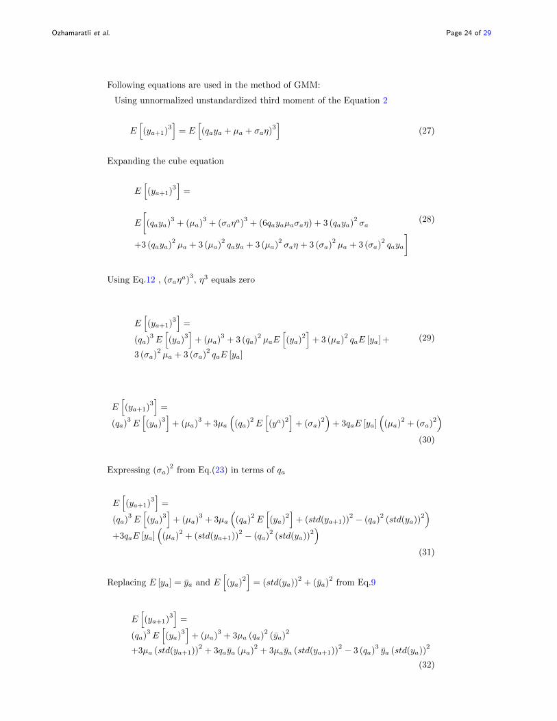
Following equations are used in the method of GMM:

Using unnormalized unstandardized third moment of the Equation 2

E[(ya+1)

3]

= E[(qaya + µa + σaη)

3]

(27)

Expanding the cube equation

E[(ya+1)

3]

=

E

[(qaya)

3+ (µa)

3+ (σaη

a)3

+ (6qayaµaσaη) + 3 (qaya)2σa

+3 (qaya)2µa + 3 (µa)

2qaya + 3 (µa)

2σaη + 3 (σa)

2µa + 3 (σa)

2qaya

] (28)

Using Eq.12 , (σaηa)

3, η3 equals zero

E[(ya+1)

3]

=

(qa)3E[(ya)

3]

+ (µa)3

+ 3 (qa)2µaE

[(ya)

2]

+ 3 (µa)2qaE [ya] +

3 (σa)2µa + 3 (σa)

2qaE [ya]

(29)

E[(ya+1)

3]

=

(qa)3E[(ya)

3]

+ (µa)3

+ 3µa

((qa)

2E[(ya)

2]

+ (σa)2)

+ 3qaE [ya](

(µa)2

+ (σa)2)

(30)

Expressing (σa)2

from Eq.(23) in terms of qa

E[(ya+1)

3]

=

(qa)3E[(ya)

3]

+ (µa)3

+ 3µa

((qa)

2E[(ya)

2]

+ (std(ya+1))2 − (qa)

2(std(ya))

2)

+3qaE [ya](

(µa)2

+ (std(ya+1))2 − (qa)

2(std(ya))

2)

(31)

Replacing E [ya] = ya and E[(ya)

2]

= (std(ya))2

+ (ya)2

from Eq.9

E[(ya+1)

3]

=

(qa)3E[(ya)

3]

+ (µa)3

+ 3µa (qa)2

(ya)2

+3µa (std(ya+1))2

+ 3qaya (µa)2

+ 3µaya (std(ya+1))2 − 3 (qa)

3ya (std(ya))

2

(32)


Expressing µa from Eq.(4) in terms of qa

E[(ya+1)

3]

=

(qa)3E[(ya)

3]

+ (ya+1 − qaya)3

+ 3 (ya+1 − qaya) (std(ya+1))2

+3qaya (ya+1 − qaya)2

+ 3qaya (std(ya+1))2 − 3 (qa)

3ya (std(ya))

2

(33)

Expressing in the form of cubic polynomial equation of qa

0 =

(qa)3(E[(ya)

3]− (ya)

3 − 3ya (std(ya))2)

+ (qa)2(

3ya+1 (ya)2 − 6 (ya)

2ya+1

)+ (qa)

(3 (µa+1)

2ya − 3ya (std(ya+1))

2+ 3ya (ya+1)

2+ 3ya (std(ya+1))

2)

+ (ya+1)3

+ 3ya+1 (std(ya+1))2 − E

[(ya+1)

3]

(34)

This equation can be solved for qa corresponding each age group. Cardano solution

for cubic equations guarantees single real root to exist, the other two complex roots

that Cardano solution provides are not used. Both of the σa = std(ya) and GMM

estimation techniques can use the following equations for determining the µa and

σa: For (qa)1 and (qa)2 according to Eq.(4):

µa = ya+1 − qaya (35)

The σ2a can also be expressed in terms of qa, using Eq.(4) :

σ2a = (∆a+1)

2 − q2a (∆a)2 −

(ya+1 − qaµ2

)2 − 2qa (ya+1 − qaya) ya (36)

7.3 Analysis BHPS - Joint Distribution of Age and Income for Observed and

Simulated Data

The parameters are estimated with LSM.


(a) Wave 1991 JDF of ObservedData.

(b) Wave 1991 JDF of Sim Data

(c) Wave 1992 JDF of ObservedData.

(d) Wave 1992 JDF of Sim Data

(e) Wave 1993 JDF of ObservedData.

(f) Wave 1993 JDF of Sim Data

(g) Wave 1994 JDF of ObservedData.

(h) Wave 1994 JDF of Sim Data

(i) Wave 1995 JDF of ObservedData.

(j) Wave 1995 JDF of Sim Data

Figure 13: JDF for Waves 1991-1995


























(a) Wave 2006 JDF of Observed Data. (b) Wave 2006 JDF of Sim Data

(c) Wave 2007 JDF of Observed Data. (d) Wave 2007 JDF of Sim Data

(e) Wave 2008 JDF of Observed Data. (f) Waves 2008 JDF of Sim Data


Documents

A generative model for age and income distribution