Embed Size (px)
Citation preview

A Generalized Linear Model
for Poisson Response Data
Copyright c©2015 Dan Nettleton (Iowa State University) Statistics 510 1 / 69

An Example Experiment
Consider an experiment designed to evaluate the effectivenessof an anti-fungal chemical on plants.
A total of 60 plant leaves were randomly assigned to treatmentwith 0, 5, 10, 15, 20, or 25 units of the anti-fungal chemical, with10 plant leaves for each amount of anti-fungal chemical.
All leaves were infected with a fungus.
Following a two-week period, the leaves were studied under amicroscope, and the number of infected cells was counted andrecorded for each leaf.
Copyright c©2015 Dan Nettleton (Iowa State University) Statistics 510 2 / 69

●
●
●
●
●
●
●
●
●
●
●●
●
●
●
●
●●
●
●
●●
●
●
●
●
●●●
●●
●
●
●
●
●●●●
● ●
●●●●●●●●● ●●●●
●●●●●●
0 5 10 15 20 25
050
100
150
200
Amount of Anti−Fungal Treatment
Num
ber
of In
fect
ed C
ells
Copyright c©2015 Dan Nettleton (Iowa State University) Statistics 510 3 / 69
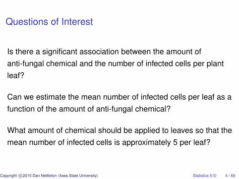
Questions of Interest
Is there a significant association between the amount ofanti-fungal chemical and the number of infected cells per plantleaf?
Can we estimate the mean number of infected cells per leaf as afunction of the amount of anti-fungal chemical?
What amount of chemical should be applied to leaves so that themean number of infected cells is approximately 5 per leaf?
Copyright c©2015 Dan Nettleton (Iowa State University) Statistics 510 4 / 69

A Generalized Linear Model for Poisson Count Data
For all i = 1, ..., n,
yi ∼ Poisson(λi),
log(λi) = x′iβ,
and y1, ..., yn are independent.
Copyright c©2015 Dan Nettleton (Iowa State University) Statistics 510 5 / 69

The Poisson Distribution
Recall that for yi ∼ Poisson(λi), the probability mass
function of yi is
P(yi = y) =
{λy
i exp(−λi)y! for y ∈ {0, 1, 2, ...}
0 otherwise,
E(yi) = λi, and Var(yi) = λi.
Copyright c©2015 Dan Nettleton (Iowa State University) Statistics 510 6 / 69

The Poisson Log Likelihood for the Generalized LM
The Poisson log likelihood function is
`(β | y) =n∑
i=1
[yi log(λi)− λi − log(yi!)]
=n∑
i=1
[yi x′iβ − exp(x′iβ)− log(yi!)].
Copyright c©2015 Dan Nettleton (Iowa State University) Statistics 510 7 / 69

Inference for the Poisson Generalized LM
The function `(β | y) can be maximized over β ∈ Rp
using Fisher’s scoring method to obtain an MLE β.
An estimate of the inverse Fisher information matrix
can be used for Wald inference concerning β.
Alternatively, we can conduct likelihood ratio based
inference of reduced vs. full models.
Copyright c©2015 Dan Nettleton (Iowa State University) Statistics 510 8 / 69

Interpretation of Parameters
Let x = [x1, x2, . . . , xj−1, xj , xj+1, . . . , xp]′.
Let x = [x1, x2, . . . , xj−1, xj + 1, xj+1, . . . , xp]′.
In other words, x is the same as x except that the jth
explanatory variable has been increased by one unit.
Let λ = exp(x′β) and λ = exp(x′β).
Copyright c©2015 Dan Nettleton (Iowa State University) Statistics 510 9 / 69

Ratio of Means
λ/λ = exp(x′β)/ exp(x′β)
= exp(x′β − x′β}
= exp{(xj + 1)βj − xjβj}
= exp(βj).
Copyright c©2015 Dan Nettleton (Iowa State University) Statistics 510 10 / 69

Thus, λ = exp(βj)λ.
All other explanatory variables held constant, the
mean response at xj + 1 is exp(βj) times the mean
response at xj.
This is true regardless of the initial value xj.
Copyright c©2015 Dan Nettleton (Iowa State University) Statistics 510 11 / 69
A one unit increase in the jth explanatory variable
(with all other explanatory variables held constant) is
associated with a multiplicative change in the mean
response by the factor exp(βj).
Copyright c©2015 Dan Nettleton (Iowa State University) Statistics 510 12 / 69

If (Lj,Uj) is a 100(1− α)% confidence interval for βj,
then
(exp(Lj), exp(Uj))
is a 100(1− α)% confidence interval for exp(βj).
Copyright c©2015 Dan Nettleton (Iowa State University) Statistics 510 13 / 69
Also, note that if (L,U) is a 100(1− α)% confidence
interval for x′β, then a 100(1− α)% confidence
interval for λ = exp(x′β) is
(exp(L), exp(U)) .
Copyright c©2015 Dan Nettleton (Iowa State University) Statistics 510 14 / 69

A Generalized LM for the Anti-Fungal Experiment
For i = 1, ..., 60, let yi denote the number of infected
cells for leaf i. Suppose y1, . . . , y60 are independent,
yi ∼ Poisson(λi), and
log(λi) = β0 + β1xi,
where xi denotes the amount of anti-fungal chemical
applied to leaf i.
Copyright c©2015 Dan Nettleton (Iowa State University) Statistics 510 15 / 69

> o=glm(y˜x,family=poisson(link = "log"))
> summary(o)
Call:
glm(formula = y ˜ x, family = poisson(link = "log"))
Deviance Residuals:
Min 1Q Median 3Q Max
-7.8363 -1.6715 -0.3411 1.2467 12.3127
Copyright c©2015 Dan Nettleton (Iowa State University) Statistics 510 16 / 69

Coefficients:
Estimate Std. Error z value Pr(>|z|)
(Intercept) 4.373003 0.032434 134.83 <2e-16 ***
x -0.162011 0.004933 -32.84 <2e-16 ***
---
Signif. codes: 0 *** 0.001 ** 0.01 * 0.05 . 0.1 1
(Dispersion parameter for poisson family taken to be 1)
Copyright c©2015 Dan Nettleton (Iowa State University) Statistics 510 17 / 69

Null deviance: 2314.87 on 59 degrees of freedom
Residual deviance: 614.65 on 58 degrees of freedom
AIC: 849.53
Number of Fisher Scoring iterations: 5
Copyright c©2015 Dan Nettleton (Iowa State University) Statistics 510 18 / 69

> #MLE of beta vector
> b=coef(o)
> b
(Intercept) x
4.3730032 -0.1620111
Copyright c©2015 Dan Nettleton (Iowa State University) Statistics 510 19 / 69

> #Estimated variance of the MLE
> v=vcov(o)
> v
(Intercept) x
(Intercept) 1.051970e-03 -9.179444e-05
x -9.179444e-05 2.433540e-05
Copyright c©2015 Dan Nettleton (Iowa State University) Statistics 510 20 / 69

Answering the First Question of Interest
Is there a significant association between the amount ofanti-fungal chemical and the number of infected cells per plantleaf?
The null hypothesis of no association between the amount ofanti-fungal chemical and the number of infected cells per plantleaf is H0 : β1 = 0 for our Generalized LM.
We can test this null hypothesis using either a Wald test or aLRT as follows.
Copyright c©2015 Dan Nettleton (Iowa State University) Statistics 510 21 / 69

Wald Test of H0 : β1 = 0
> #Test Statistic
> z=b[2]/sqrt(v[2,2])
> z
x
-32.84169
> #p-value
> 2*pnorm(z)
x
1.496932e-236
Copyright c©2015 Dan Nettleton (Iowa State University) Statistics 510 22 / 69

Likelihood Ratio Test of H0 : β1 = 0
> anova(o,test="Chisq")
Analysis of Deviance Table
Model: poisson, link: log
Response: y
Terms added sequentially (first to last)
Df Deviance Resid. Df Resid. Dev Pr(>Chi)
NULL 59 2314.87
x 1 1700.2 58 614.65 < 2.2e-16 ***
Copyright c©2015 Dan Nettleton (Iowa State University) Statistics 510 23 / 69

Answering the Second Question of Interest
Can we estimate the mean number of infected cells per leaf as afunction of the amount of anti-fungal chemical?
According to our Poisson Generalized LM, the mean number ofinfected cells for a leaf treated with x units of the anti-fungalchemical is
exp(β0 + β1x), which is estimated by exp(β0 + β1x).
Copyright c©2015 Dan Nettleton (Iowa State University) Statistics 510 24 / 69

We can add the estimated mean function to ourscatterplot with the following code:
xgrid=seq(0,25,by=.1)
lines(xgrid,exp(b[1]+b[2]*xgrid),col=2,lwd=1.5)
Copyright c©2015 Dan Nettleton (Iowa State University) Statistics 510 25 / 69

●
●
●
●
●
●
●
●
●
●
●●
●
●
●
●
●●
●
●
●●
●
●
●
●
●●●
●●
●
●
●
●
●●●●
● ●
●●●●●●●●● ●●●●
●●●●●●
0 5 10 15 20 25
050
100
150
200
Amount of Anti−Fungal Treatment
Num
ber
of In
fect
ed C
ells
Copyright c©2015 Dan Nettleton (Iowa State University) Statistics 510 26 / 69

Example Confidence Interval for a MeanAn approximate 95% Wald confidence interval for the meannumber of infected cells when 15 units of the chemical areapplied is (6.17, 7.89).
> cc=c(1,15)
> se=sqrt(t(cc)%*%v%*%cc)
> exp(t(cc)%*%b-2*se)
[,1]
[1,] 6.171721
> exp(t(cc)%*%b+2*se)
[,1]
[1,] 7.89079
Copyright c©2015 Dan Nettleton (Iowa State University) Statistics 510 27 / 69
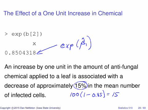
The Effect of a One Unit Increase in Chemical
> exp(b[2])
x
0.8504318
An increase by one unit in the amount of anti-fungal
chemical applied to a leaf is associated with a
decrease of approximately 15% in the mean number
of infected cells.
Copyright c©2015 Dan Nettleton (Iowa State University) Statistics 510 28 / 69

Confidence Interval for the Multiplicative Factor
> c(exp(b[2]-2*sqrt(v[2,2])),exp(b[2]+2*sqrt(v[2,2])))
x x
0.8420825 0.8588638
An approximated 95% confidence interval for the mean
associated with x + 1 units of chemical divided by the mean
associated with x units of the chemical (λ/λ) is (0.842, 0.859).
Copyright c©2015 Dan Nettleton (Iowa State University) Statistics 510 29 / 69

Answering the Third Question of Interest
What amount of chemical should be applied to leaves so that themean number of infected cells is approximately 5 per leaf?
λ = 5 ⇐⇒ log(λ) = log(5)
⇐⇒ x′β = log(5)
⇐⇒ β0 + β1x = log(5)
⇐⇒ x = (log(5)− β0)/β1
Thus, we seek an estimate of the nonlinear function of β givenby
h(β) = (log(5)− β0)/β1.
Copyright c©2015 Dan Nettleton (Iowa State University) Statistics 510 30 / 69

Answering the Third Question of Interest
By the invariance property, the MLE of h(β) is
h(β) = h(β) = (log(5)− β0)/β1.
By the Delta Method, h(β) is approximately normal with meanh(β) and variance
Var(h(β)) = D′Var(β)D,
where
D′ =
[∂h(β)∂β0
∣∣∣∣β=β
,∂h(β)∂β1
∣∣∣∣β=β
].
Copyright c©2015 Dan Nettleton (Iowa State University) Statistics 510 31 / 69
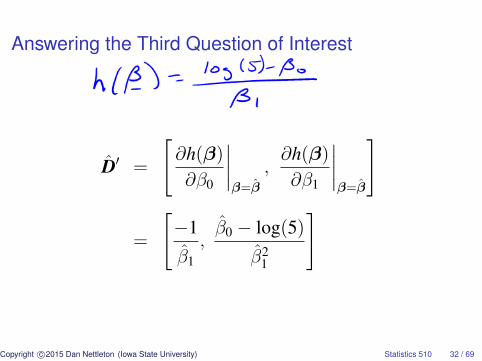
Answering the Third Question of Interest
D′ =
[∂h(β)∂β0
∣∣∣∣β=β
,∂h(β)∂β1
∣∣∣∣β=β
]
=
[−1
β1,β0 − log(5)
β21
]
Copyright c©2015 Dan Nettleton (Iowa State University) Statistics 510 32 / 69

> h=(log(5)-b[1])/b[2]
> h
(Intercept)
17.05788
>
> Dhat=c(-1/b[2],(b[1]-log(5))/b[2]ˆ2)
>
> seh=sqrt(t(Dhat)%*%v%*%Dhat)
>
> ci=c(h-2*seh,h+2*seh)
> ci
[1] 16.18486 17.93090
Copyright c©2015 Dan Nettleton (Iowa State University) Statistics 510 33 / 69

Answering the Third Question of Interest
The estimated amount of chemical that should be
applied to leaves so that the mean number of infected
cells is approximately 5 per leaf is 17.1 units.
An approximate 95% confidence interval for the
required amount of chemical is 16.2 to 17.9 units.
Copyright c©2015 Dan Nettleton (Iowa State University) Statistics 510 34 / 69

plot(x,y,xlab="Level of Anti-Fungal Treatment",
ylab="Number of Infected Cells",col=4,cex.lab=1.5,
xlim=c(14,21),ylim=c(0,18))
xgrid=seq(0,25,by=.1)
lines(xgrid,exp(b[1]+b[2]*xgrid),col=2,lwd=1.5)
abline(h=5,lty=2)
lines(c(h,h),c(-1,5),lwd=1.5)
lines(c(ci[1],ci[1]),c(-1,5),lwd=1.5,col="purple")
lines(c(ci[2],ci[2]),c(-1,5),lwd=1.5,col="purple")
Copyright c©2015 Dan Nettleton (Iowa State University) Statistics 510 35 / 69

●
●
●
●
●
●
●
●
●
●
●
●●
●
●●
●
●
●
●
14 15 16 17 18 19 20 21
05
1015
Amount of Anti−Fungal Treatment
Num
ber
of In
fect
ed C
ells
Copyright c©2015 Dan Nettleton (Iowa State University) Statistics 510 36 / 69

Checking for Lack of Fit
We can compare the fit of a Poisson Generalized LM
to the fit of a saturated model.
The saturated model uses one parameter for each
observation.
In this case, the saturated model has one free
parameter λi for each yi.
Copyright c©2015 Dan Nettleton (Iowa State University) Statistics 510 37 / 69

Poisson Generalized LM
yi ∼ Poisson(λi)
y1, ..., yn independent
λi = exp(x′iβ)
for some β ∈ Rp
p parameters
Saturated Model
yi ∼ Poisson(λi)
y1, ..., yn independent
λi ∈ [0,∞) for i = 1, ..., n
with no other restrictions
n parameters
Copyright c©2015 Dan Nettleton (Iowa State University) Statistics 510 38 / 69

For all i = 1, . . . , n,
the MLE of λi under the Poisson Generalized LM is
λi = exp(x′iβ),
and the MLE of λi under the saturated model is
simply yi.
Copyright c©2015 Dan Nettleton (Iowa State University) Statistics 510 39 / 69

Then the likelihood ratio statistic for testing the
Poisson Generalized LM as the reduced model vs.
the saturated model as the full model is
2n∑
i=1
[yi log
(yi
λi
)− (yi − λi)
].
This is the Deviance Statistic for the Poisson case.
Copyright c©2015 Dan Nettleton (Iowa State University) Statistics 510 40 / 69
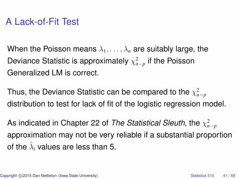
A Lack-of-Fit Test
When the Poisson means λ1, . . . , λn are suitably large, theDeviance Statistic is approximately χ2
n−p if the PoissonGeneralized LM is correct.
Thus, the Deviance Statistic can be compared to the χ2n−p
distribution to test for lack of fit of the logistic regression model.
As indicated in Chapter 22 of The Statistical Sleuth, the χ2n−p
approximation may not be very reliable if a substantial proportionof the λi values are less than 5.
Copyright c©2015 Dan Nettleton (Iowa State University) Statistics 510 41 / 69

Deviance Residuals
In the Poisson case, the deviance residuals are given
by
di ≡ sign(yi − λi)
√2[
yi log(
yi
λi
)− (yi − λi)
].
The Deviance Statistic is the sum of the squared
deviance residuals (∑n
i=1 d2i ).
Copyright c©2015 Dan Nettleton (Iowa State University) Statistics 510 42 / 69
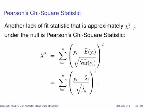
Pearson’s Chi-Square Statistic
Another lack of fit statistic that is approximately χ2n−p
under the null is Pearson’s Chi-Square Statistic:
X2 =n∑
i=1
yi − E(yi)√Var(yi)
2
=n∑
i=1
yi − λi√λi
2
.
Copyright c©2015 Dan Nettleton (Iowa State University) Statistics 510 43 / 69
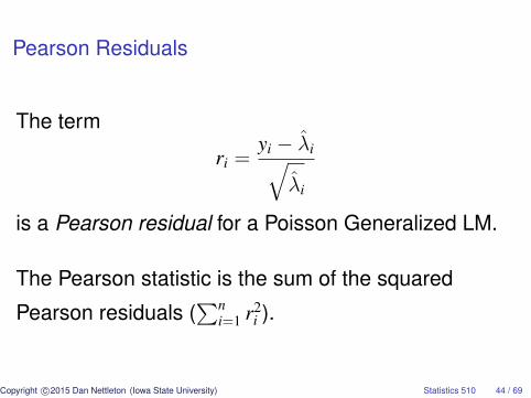
Pearson Residuals
The term
ri =yi − λi√
λi
is a Pearson residual for a Poisson Generalized LM.
The Pearson statistic is the sum of the squared
Pearson residuals (∑n
i=1 r2i ).
Copyright c©2015 Dan Nettleton (Iowa State University) Statistics 510 44 / 69

Residual Diagnostics
For large λi, both di and ri should be approximately
distributed as standard normal random variables if the
Poisson Generalized LM is correct.
Thus, either set of residuals can be used to diagnose
problems with model fit by, e.g., identifying outlying
observations.
Copyright c©2015 Dan Nettleton (Iowa State University) Statistics 510 45 / 69

R Code to Generate a Deviance Residual Plot
d=resid(o,type="deviance")
plot(fitted(o),d,
xlab="Estimated Mean",
ylab="Deviance Residual",
cex.lab=1.4,
pch=16,col=4)
abline(h=0,lty=2)
Copyright c©2015 Dan Nettleton (Iowa State University) Statistics 510 46 / 69

●
●
●
●
●
●
●
●
●
●
●
●
●
●
●
●
●
●
●
●●
●
●
●
●
●
●●
●
●
●
●
●
●
●
●●
●●
●
●
●●
●
●●
●
●
●
●●
●●●
●
●
●
●
●
●
0 20 40 60 80
−5
05
10
Estimated Mean
Dev
ianc
e R
esid
ual
Copyright c©2015 Dan Nettleton (Iowa State University) Statistics 510 47 / 69

R Code to Generate a Pearson Residual Plot
r=resid(o,type="pearson")
plot(fitted(o),r,
xlab="Estimated Mean",
ylab="Pearson Residual",
cex.lab=1.4,
pch=16,col=4)
abline(h=0,lty=2)
Copyright c©2015 Dan Nettleton (Iowa State University) Statistics 510 48 / 69

●
●
●
●
●
●
●
●
●
●
●●
●
●
●
●
●
●
●
●●
●
●
●
●
●
●●
●
●
●
●
●
●
●
●●
●●
●
●
●●
●
●●
●
●
●
●●
●●●
●
●
●
●
●
●
0 20 40 60 80
−5
05
1015
Estimated Mean
Pea
rson
Res
idua
l
Copyright c©2015 Dan Nettleton (Iowa State University) Statistics 510 49 / 69

Overdispersion
In the Generalized Linear Models framework, its often
the case that Var(y) is a function of E(y).
For the Poisson case,
Var(y) = E(y) = λ.
Copyright c©2015 Dan Nettleton (Iowa State University) Statistics 510 50 / 69

Thus, when we fit a Poisson Generalized LM and
obtain estimates of the mean of the response, we get
estimates of the variance of the response as well.
If the variability of our response is greater than we
should expect based on our estimates of the mean,
we say that there is overdispersion.
Copyright c©2015 Dan Nettleton (Iowa State University) Statistics 510 51 / 69

●
●
●
●
●
●
●
●
●
●
●●
●
●
●
●
●●
●
●
●●
●
●
●
●
●●●
●●
●
●
●
●
●●●●
● ●
●●●●●●●●● ●●●●
●●●●●●
0 5 10 15 20 25
050
100
150
200
Amount of Anti−Fungal Treatment
Num
ber
of In
fect
ed C
ells
Copyright c©2015 Dan Nettleton (Iowa State University) Statistics 510 52 / 69

●
●
●
●
●
●
●
●
●
●
●●
●
●
●
●
●
●
●
●●
●
●
●
●
●
●●
●
●
●
●
●
●
●
●●
●●
●
●
●●
●
●●
●
●
●
●●
●●●
●
●
●
●
●
●
0 20 40 60 80
−5
05
1015
Estimated Mean
Pea
rson
Res
idua
l
Copyright c©2015 Dan Nettleton (Iowa State University) Statistics 510 53 / 69

If either the Deviance Statistic or the Pearson
Chi-Square Statistic suggests a lack of fit that cannot
be explained by other reasons (e.g., poor model for
the mean or a few extreme outliers), overdispersion
may be the problem.
Copyright c©2015 Dan Nettleton (Iowa State University) Statistics 510 54 / 69
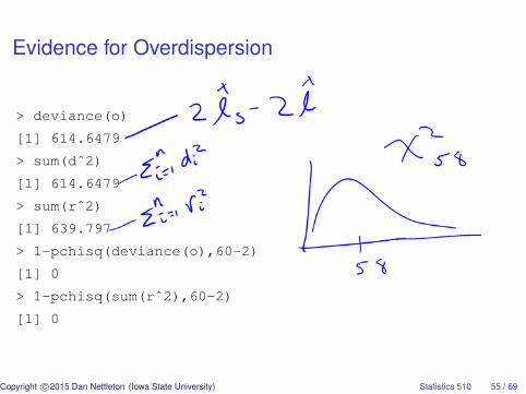
Evidence for Overdispersion
> deviance(o)
[1] 614.6479
> sum(dˆ2)
[1] 614.6479
> sum(rˆ2)
[1] 639.797
> 1-pchisq(deviance(o),60-2)
[1] 0
> 1-pchisq(sum(rˆ2),60-2)
[1] 0
Copyright c©2015 Dan Nettleton (Iowa State University) Statistics 510 55 / 69

Quasi-Likelihood (QL) Inference
If there is overdispersion, a quasi-likelihood approach
may be used.
In the Poisson case, we make all the same
assumptions as before except that we assume
Var(yi) = φλi
for some unknown dispersion parameter φ > 1.
Copyright c©2015 Dan Nettleton (Iowa State University) Statistics 510 56 / 69

The dispersion parameter φ can be estimated by
φ =
∑ni=1 d2
i
n− p
or
φ =
n∑i=1
r2i
n− p.
Copyright c©2015 Dan Nettleton (Iowa State University) Statistics 510 57 / 69

All analyses are as before except that
1 The estimated variance of β is multiplied by φ.
2 For Wald type inferences, the standard normal null
distribution is replaced by t with n− p degrees of
freedom.
3 Any test statistic T that was assumed χ2q under H0
is replaced with T/(qφ) and compared to an F
distribution with q and n− p degrees of freedom.Copyright c©2015 Dan Nettleton (Iowa State University) Statistics 510 58 / 69

These changes to the inference strategy in the
presence of overdispersion are analogous to the
changes that would take place in normal theory
Gauss-Markov linear model analysis if we switched
from assuming σ2 were known to be 1 to assuming σ2
were unknown and estimating it with MSE.
(Here φ is like σ2 and φ is like MSE.)
Copyright c©2015 Dan Nettleton (Iowa State University) Statistics 510 59 / 69

Whether there is overdispersion or not, all the usual
ways of conducting generalized linear models
inference are approximate except for the special case
of normal theory linear models.
Copyright c©2015 Dan Nettleton (Iowa State University) Statistics 510 60 / 69

QL Analysis of the Fungal Infection Data
> #Estimates of the dispersion parameter
>
> deviance(o)/df.residual(o)
[1] 10.59738
>
> sum(rˆ2)/df.residual(o)
[1] 11.03098
Copyright c©2015 Dan Nettleton (Iowa State University) Statistics 510 61 / 69

> oq=glm(y˜x,family=quasipoisson(link = "log"))
> summary(oq)
Call:
glm(formula = y ˜ x, family = quasipoisson(link = "log"))
Deviance Residuals:
Min 1Q Median 3Q Max
-7.8363 -1.6715 -0.3411 1.2467 12.3127
Copyright c©2015 Dan Nettleton (Iowa State University) Statistics 510 62 / 69

Coefficients:
Estimate Std. Error t value Pr(>|t|)
(Intercept) 4.37300 0.10772 40.595 < 2e-16 ***
x -0.16201 0.01638 -9.888 4.7e-14 ***
---
Signif. codes: 0 *** 0.001 ** 0.01 * 0.05 . 0.1 1
(Dispersion parameter for quasipoisson family
taken to be 11.03098)
Copyright c©2015 Dan Nettleton (Iowa State University) Statistics 510 63 / 69

Null deviance: 2314.87 on 59 degrees of freedom
Residual deviance: 614.65 on 58 degrees of freedom
AIC: NA
Number of Fisher Scoring iterations: 5
Copyright c©2015 Dan Nettleton (Iowa State University) Statistics 510 64 / 69
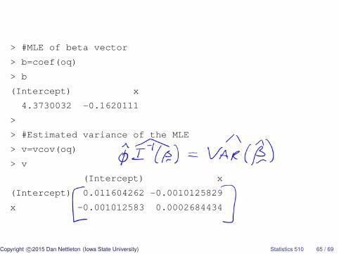
> #MLE of beta vector
> b=coef(oq)
> b
(Intercept) x
4.3730032 -0.1620111
>
> #Estimated variance of the MLE
> v=vcov(oq)
> v
(Intercept) x
(Intercept) 0.011604262 -0.0010125829
x -0.001012583 0.0002684434
Copyright c©2015 Dan Nettleton (Iowa State University) Statistics 510 65 / 69

> #Test Statistic
> tstat=b[2]/sqrt(v[2,2])
> tstat
x
-9.888225
>
> #p-value
> 2*pt(tstat,60-2)
x
4.700095e-14
Copyright c©2015 Dan Nettleton (Iowa State University) Statistics 510 66 / 69

> #Likelihood Ratio Test
> anova(oq,test="F")
Analysis of Deviance Table
Model: quasipoisson, link: log
Response: y
Terms added sequentially (first to last)
Df Deviance Resid. Df Resid. Dev F Pr(>F)
NULL 59 2314.87
x 1 1700.2 58 614.65 154.13 < 2.2e-16 ***
Copyright c©2015 Dan Nettleton (Iowa State University) Statistics 510 67 / 69

Exponential Dispersion Families
The normal, Bernoulli, binomial, and Poisson families ofdistributions can each be characterized as an exponentialdispersion family of distributions with a probability densityfunction or probability mass function of the form
exp{
yθ − b(θ)a(φ)
+ c(y, φ)},
where a(·), b(·), and c(·) are specific functions, θ is an unknownparameter that is a function of the mean, and φ is a dispersionparameter that may or may not be known.
Copyright c©2015 Dan Nettleton (Iowa State University) Statistics 510 68 / 69

Exponential Dispersion Families
The gamma and inverse Gaussian families of distributions areother example distributions sometimes useful for modeling datathat can be characterized as exponential dispersion families.
Generalized Linear Models for gamma and inverse Gaussiandistributions will be discussed in STAT520 – along with moredetails about normal, Bernoulli, binomial, and PoissonGeneralized Linear Models.
Copyright c©2015 Dan Nettleton (Iowa State University) Statistics 510 69 / 69