1  

Photosynthesis Research 1

A generalised dynamic model of leaf-level C3 photosynthesis 2

combining light and dark reactions with stomatal behaviour 3

Chandra Bellasio 4

Research School of Biology, Australian National University, Acton, ACT, 2601 Australia 5

University of the Balearic Islands 07122 Palma, Illes Balears, Spain 6

Trees and Timber institute, National Research Council of Italy, 50019 Sesto Fiorentino (Florence) 7

chandra.bellasio@anu.edu.au ORCiD 0000-0002-3865-7521 8

Running title 9

Dynamic model of C3 leaf assimilation 10

Keywords 11

Mechanistic model, Microsoft® Excel®, stomatal model, time, transients, stomatal conductance, 12

assimilation, photorespiration, light fleck. 13

Acknowledgments 14

I am deeply grateful to the Editor of this special issue, Nerea Ubierna Lopez, for editing that 15

improved the clarity and readability, to Joe Quirk for a substantial contribution to writing the first 16

version, I thank Ross Deans (Australian National University, ANU) for unpublished spinach leaf 17

gas exchange data, and Florian Busch (ANU) for help, review, and critical discussion. I am funded 18

through a H2020 Marie Skłodowska-Curie individual fellowship (DILIPHO, ID: 702755). 19

I have no conflict of interest. 20

  21

 

2  

Abstract 22

Global food demand is rising, impelling us to develop strategies for improving the efficiency of 23

photosynthesis. Classical photosynthesis models based on steady state assumptions are inherently 24

unsuitable for assessing biochemical and stomatal responses to rapid variations in environmental 25

drivers. To identify strategies to increase photosynthetic efficiency, we need models that account 26

for the timing of CO2 assimilation responses to dynamic environmental stimuli. Herein, I present a 27

dynamic process-based photosynthetic model for C3 leaves. The model incorporates both light and 28

dark reactions, coupled with a hydro-mechanical model of stomatal behaviour. The model achieved 29

a stable and realistic rate of light-saturated CO2 assimilation and stomatal conductance. 30

Additionally, it replicated complete typical assimilatory response curves (stepwise change in CO2 31

and light intensity at different oxygen levels) featuring both short lag times and full photosynthetic 32

acclimation. The model also successfully replicated transient responses to changes in light intensity 33

(light flecks), CO2 concentration, and atmospheric oxygen concentration. This dynamic model is 34

suitable for detailed ecophysiological studies and has potential for superseding the long-dominant 35

steady-state approach to photosynthesis modelling. The model runs as a stand-alone workbook in 36

Microsoft® Excel® and is freely available to download along with a video tutorial. 37

Introduction 38

The pace of increases in crop yields has stalled over recent decades, urging researchers to develop 39

innovative solutions to safeguard the productivity necessary to sustain expected future global 40

demand for food and feed (Ray et al. 2012; Ray et al. 2013). The photosynthetic efficiency of C3 41

crop plants falls short of theoretical potentials and is little or negatively affected by selective 42

breeding (Long et al. 2015), making efficiency gains a key aim for improving yields from existing 43

agricultural land (Taylor and Long 2017). Photosynthetic responses to dynamic environmental 44

drivers are increasingly recognised as an area where photosynthetic efficiency can be improved by 45

minimising the assimilatory and, or stomatal lag response(s) to environmental fluctuations, 46

particularly light intensity (Kaiser et al. 2014; Lawson and Blatt 2014). 47

Leaves may experience large transient variations in light intensity (measured as photosynthetic 48

photon flux density, PPFD) as they move into the shade of leaves higher in the canopy and clouds 49

move overhead to create light- and shade-flecks of varying intensity and spectral quality (Bellasio 50

and Griffiths 2014; Pearcy et al. 1985; Pearcy 1990; Valladares et al. 1997). Shaded leaves can 51

contribute up to 50% of canopy photosynthesis (Long 1993; Long et al. 1996) and accurate 52

quantification of CO2 assimilation (A) requires modelling of leaf responses to fluctuations in the 53

canopy light environment (Allen and Richardson 1968; Song et al. 2013). In addition, atmospheric 54

CO2 concentration (Ca) can vary locally under natural field conditions, but variability in Ca is more 55

frequent and pronounced when [CO2] is experimentally enriched (Hendrey et al. 1997). 56

 

3  

Stomata and photosynthesis respond continuously to environmental changes, but stomatal 57

adjustments, which regulate the diffusion of CO2 into the leaf and the conductance of water vapour 58

to the atmosphere (gS), can be an order of magnitude slower than assimilatory responses 59

(McAusland et al. 2016). This lack of coordination between carbon gains (A) and water losses (E) 60

often results in suboptimal water-use efficiency (WUE = A/E) and photosynthetic shortfalls 61

(Lawson and Blatt 2014; Bellasio et al. 2017). Further, A may be biochemically limited due to a lag 62

time in the induction of biochemical activity following environmental fluctuations (Naumburg and 63

Ellsworth 2002; Taylor and Long 2017). By improving the speed at which the photosynthetic 64

machinery responds and adjusts to fluctuating environmental conditions, substantial accrual of 65

marginal gains in A and water savings over time are possible (Bellasio et al. 2017; Lawson and Blatt 66

2014; McAusland et al. 2016; Way and Pearcy 2012). 67

Most photosynthesis models, used at leaf level and broader scales, are based on steady state 68

principles [for review (Bellasio et al. 2016b; Bellasio et al. 2016a)]. Assimilation is often predicted 69

using steady-state sub-models rooted in the Farquhar et al. (1980) framework, which have since 70

been updated (Busch et al. 2017; Yin et al. 2014). Steady-state photosynthesis models tend to 71

overestimate integrated A under fluctuating PPFD (Kaiser et al. 2014), but also under variable Ca 72

(Hendrey et al. 1997). This results, for instance, in poor understanding of plant growth and 73

acclimation responses in CO2 enrichment experiments, particularly under free air CO2 enrichment 74

(FACE) conditions (Long et al. 2006). This confounds the interpretation of experimental findings 75

and hinders prediction of vegetation responses to rising CO2 levels in the future. Moreover, 76

incorporation of the latest developments in plant manipulation, including the effect of a modified 77

reductive pentose phosphate pathway [RPP, (Driever et al. 2017)] and light reaction processes 78

(Kromdijk et al. 2016), require further biochemical complexity than that of traditional models. In 79

broader scale vegetation modelling, photosynthesis models are coupled with models characterising 80

stomatal behaviour (Berry et al. 2010; Beerling 2015; Bonan et al. 2014; Ostle et al. 2009; Sato et 81

al. 2015). The stomatal sub-models generally estimate gS empirically from environmental or 82

internal variables rather than from process-based mechanistic principles (Damour et al. 2010). 83

Empirical models may lose accuracy as simulated conditions deviate further from those under 84

which the models were calibrated (Way et al. 2011) and then cannot provide insight into underlying 85

physiological mechanisms (Buckley 2017). 86

Dynamic models characterise photosynthesis and stomatal behaviour under non steady-state 87

conditions. Although dynamic models of photosynthesis and gS exist [e.g. (Kirschbaum et al. 1997; 88

Laisk and Eichelmann 1989)], their application has been limited by the accessibility of the code or 89

because their treatment of photosynthetic processes is either phenomenological (Vialet-Chabrand et 90

al. 2016; McAusland et al. 2016), elementary (Pearcy et al. 1997; Gross et al. 1991), or so complex 91

as to require dedicated software and high-capability computing (Laisk et al. 2009; Wang et al. 92

 

4  

2014a; Wang et al. 2014b; Zhu et al. 2013; Zhu et al. 2007). Consequently, most studies, including 93

those simulating dynamic conditions, have used steady-state models [e.g. (Taylor and Long 2017)]. 94

Here I developed a biochemical, process-based framework for modelling photosynthetic dark 95

reactions that is incorporated with light reactions and coupled to a mechanistic hydro-mechanical 96

model of stomatal behaviour. I demonstrate its applicability using a range of examples including 97

classical A–PPFD and A–Ci response curves, a mid-term acclimation to variable Ca and PPFD, and 98

response to rapid transitions in light intensity and oxygen concentration. To maximise the potential 99

user base of the model, I coded and developed it in a Microsoft® Excel® workbook, which is openly 100

available from the Supplementary Information along with a video user guide. 101

Model development 102

Overview 103

A process-based, stock-and-flow model of leaf-level C3 photosynthesis that runs in Excel® was 104

developed incorporating leaf-level diffusion with a comprehensive treatment of assimilatory 105

biochemistry and stomatal behaviour (Figure 1, equations are detailed in the Appendix). The 106

modelled leaf consists of three compartments: the atmosphere, intercellular space and mesophyll. 107

The processes of CO2 diffusion through stomata, and CO2 dissolution and hydration are described 108

mechanistically. To reduce computational requirements, intercellular space and mesophyll are 109

assumed uniform with no internal concentration gradients. Consequently, limitations imposed by 110

the diffusion of metabolites are not considered. This is justified by a number of studies showing 111

minimal reduction in A by heterogeneous distribution of metabolites (Wang et al. 2017; Retta et al. 112

2016; Tholen et al. 2012; Ho et al. 2015). 113

A light reactions submodel, modified from Yin et al. (2004), was used to estimate the potential 114

rates of ATP and NADPH production for any PPFD. In the original Yin et al. (2004) formulation, 115

the ratio of ATP to NADPH production rates could be adjusted by varying the cyclic electron flow 116

rate (CEF, although this is close to zero for C3 types). However, up–regulating CEF required 117

additional light to be absorbed by photosystem I (PSI) because a constant electron flow through 118

PSII (J2) was assumed to facilitate implementation with fluorescence measurements. Here, a 119

constant level of total light absorbed by PSI and PSII was used and was partitioned between 120

photosystems using Yin et al. (2004) equations but modified (see Figure 2) to account for the 121

presence of the nicotinamide adenine dinucleotide (NADH) dehydrogenase–like (NDH) complex 122

(Ishikawa et al. 2016; Yamori and Shikanai 2016). 123

After passing through PSI, electrons are either cycled to plastoquinone, used by alternative sinks 124

(JPseudocyc includes all sinks that are not assimilatory dark reactions, such as O2 and NO3-), or used to 125

reduce NADP+ (JNADPH is the NADPH used in assimilatory dark reactions). In this way, the power 126

requirements for nitrogen reduction (Busch et al. 2017) are explicitly accounted for as a fraction of 127

 

5  

pseudo–cyclic electron flow (fPseudocyc NR), in line with Yin and Struik (2012). The remainder is 128

consumed by the water–water cycle, also modelled explicitly. Although fPseudocyc has a small value 129

[~0.1, (Yin et al. 2004; Yin and Struik 2012)], its inclusion is important, as it influences the 130

ATP/NADP ratio. The total ATP production rate (JATP) was obtained by summing the proton flow 131

to the lumen and dividing by h, the number of protons required by ATP synthase. The potential 132

rates of ATP and NADPH production are used by ATP and NADPH synthesis, which were 133

modelled through a Michaelis–Menten kinetics function after Wang et al. (2014a). The proportion 134

of actual to potential ATP and NADPH synthesis continuously feeds back to dark reactions by 135

adjusting PSII yield [Y(II)] and the level of CEF. Time–delay functions allow simulation of 136

photosynthetic acclimation of the potential rate of ATP (JATP ) and NADPH (JNADPH) synthesis to 137

changes in PPFD. 138

A dynamic submodel of dark reactions, including key reactions involved in the RPP cycle, 139

photorespiration pathway and carbohydrate synthesis, was developed by synthesis of the model of 140

Zhu et al. (2007). This model related enzyme activity to the concentration of substrates, including 141

ATP and NADPH, and enzyme kinetic properties. Equations were simplified where possible with 142

modifications according to the theoretical work of Bellasio (2017). Metabolite flows were 143

calculated using a set of differential equations derived from the stoichiometry of Bellasio (2017) by 144

removing the assumption of steady–state. Time delay functions are used for Rubisco activation state 145

(Ract) and carbohydrate synthesis, CS. 146

The model also includes a stomatal component based on the hydro–mechanical formulation of 147

Bellasio et al. (2017), developed after Buckley et al. (2003) and Rodriguez-Dominguez et al. 148

(2016). Hydro–mechanical forcing links guard cell responses to leaf water status and turgor, which 149

are in turn related to soil water status and plant hydraulic conductance. Leaf turgor varies from a 150

maximum value (corresponding to negative osmotic potential, πe) to zero as a function of the 151

equilibrium between water demand (determined by the leaf–to–boundary layer water mole–fraction 152

gradient [DS] and gS) and water supply (determined by soil water potential, ΨSoil, and soil–to–leaf 153

hydraulic conductance [Kh]). The influence of biochemical factors relative to hydro–mechanical 154

forcing is determined by the parameter β (defined as hydromechanical/biochemical response 155

parameter), while stomatal morphology is described by χ (defined as turgor to conductance scaling 156

factor). The strength of biochemical forcing (accounting for factors such as light intensity and CO2 157

concentration) is represented by . In this formulation, was set to equal f(RuBP), a function 158

describing the degree of ribulose 1,5–bisphosphate (RuBP) saturation of RuBP 159

carboxylase/oxygenase (Rubisco) active sites, thus, is a measure of the balance between the light 160

and dark reactions of photosynthesis, in sensu Farquhar and Wong (1984). Consistent behaviour of 161

is supported via evidence suggesting that stomata respond to the supply and demand for energy 162

carriers in photosynthesis (Wong 1979; Busch 2014; Mott et al. 2014; Messinger et al. 2006) – i.e., 163

increasing with PPFD and decreasing with Ci. The use of as a predictor of stomatal behaviour is 164

 

6  

empirically based. This is justified by its capacity to predict parallel events occurring in chloroplasts 165

and guard cells, but I make no claim about whether τ offers a faithful mechanistic description of 166

stomatal behaviour [for discussions see Farquhar and Wong (1984); Bellasio et al. (2017); and 167

Buckley (2017)]. 168

Stomata respond to any perturbation with a delay due to the kinetics of adjustment of guard cell 169

osmotic pressure. The time constant for that delay is species–specific and typically differs between 170

opening and closing movements (Lawson and Blatt 2014). With the delay functions included, the 171

stomatal sub–model can be used for simulating the gS dynamic response to fast changes in 172

humidity, hydraulic conductance and ΨSoil [but see considerations on the ‘wrong way response’ 173

made in Bellasio et al. (2017)]. Yet, because changes in these inputs typically occur on timescales 174

of hours to weeks, they will be approximated by steady state behaviour, not addressed here [but see 175

Bellasio et al. (2017)]. The model should also be suitable for calculating fast dynamics of gS in 176

response to light flecks [e.g. Pearcy et al. (1997)], though gS responses shorter than one minute have 177

not yet been calibrated. 178

Parameterisation 179

Literature values for the different parameters were averaged because the aim was to simulate 180

realistic, general behaviour, not behaviour specific to a particular species or environmental 181

conditions. Values for the parameters are reported in Supplementary Tables S1 and S2. Biochemical 182

constants were primarily derived from Zhu et al. (2007) and Wang et al. (2014a and 2014b). Some 183

biochemical and electron transport parameters were taken from Bellasio et al. (2016b), or from von 184

Caemmerer (2000). Stomatal parameters were taken from, or assigned values similar to, Bellasio et 185

al. (2017). For parameterisation of combined or simplified processes, I either derived parameters 186

from the original equations or assigned plausible, physiologically realistic values. Parameters 187

defining the PPFD dependence of Rubisco activation (Eqn 19) were initially set at values from 188

Seemann et al. (1988) and adjusted by fitting the steady state PGA concentration in light curves 189

shown in Figure 4. Parameters defining the dependence of Rubisco activation on CO2 concentration 190

at the M carboxylating sites, CM (Eqn 20) were derived empirically following these considerations: 191

1) by comparing measurements and model outputs (Figure 3, Figure 4) and considering data from 192

Sage et al. (2002) I established that Rubisco is fully activated for CM above 200 µmol mol-1; 2) 193

Tangible inactivation occurs for CM below 100 µmol mol-1 (Sage et al. 2002); and 3) Activity 194

decreases to zero for [CO2] approaching zero (Portis et al. 1986), but yet a substantial residual 195

activity exists for CO2 concentration around the CO2 compensation point. The values were then 196

adjusted by fitting the steady state PGA concentration in A/Ci curves shown in Figure 4 and the 197

final values proposed are shown in Table S2. Additional parameter tuning may be required before 198

the model is applied to specific species or growth conditions. 199

 

7  

Outputs 200

At each time step, the model calculates nine metabolite stocks (expressed both as mol per metre 201

square of leaf or concentration, mM): Ci, mesophyll [CO2], bicarbonate, RuBP, PGA, 202

dihydroxyacetone phosphate (DHAP), ATP, NADPH and Ribulose 5–Phosphate (Ru5P). The 203

concentrations of inorganic phosphorus (Pi), adenosine diphosphate (ADP) and NADP are 204

calculated by subtraction from a total pool (Figure 1). From this, 12 flow rates are calculated 205

(expressed in mmol m-2 s-1 and plotted in the figures in units of mol m-2 s-1): actual ATP and 206

NADPH synthesis (vATP and vNADPH), Rubisco carboxylation and oxygenation (VC, and VO), rates of 207

glycine decarboxylase (GDC), phosphoribulokinase (RuPPhosp), PGA reduction (PR), carbohydrate 208

synthesis (CS), CO2 stomatal diffusion, CO2 dissolution, carbonic anhydrase hydration (CA), and 209

the reactions through the RPP cycle (RPP). 210

Simulations 211

A typical dynamic simulation involves first clearing any previous results, defining the initial 212

state of the leaf, including metabolite concentrations (see Supplementary Table S2), and then 213

iteratively calculating the ‘flows’ and subsequent variation in ‘stocks’. Over time, the stocks reach 214

steady state, where they depend solely on flows, but not on their initial value. A dynamic simulation 215

may involve perturbing steady state conditions, and observing how a new steady state is reached. 216

Figure S1 shows a typical trace of an output quantity (CO2 stomatal diffusion) plotted over time 217

while Ca and PPDF were varied to simulate a typical gas exchange experiment. 218

1. A–PPFD and A–Ci response curves 219

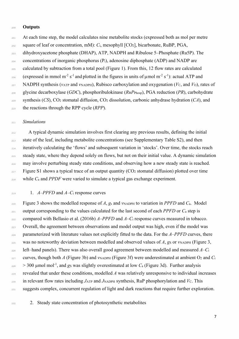
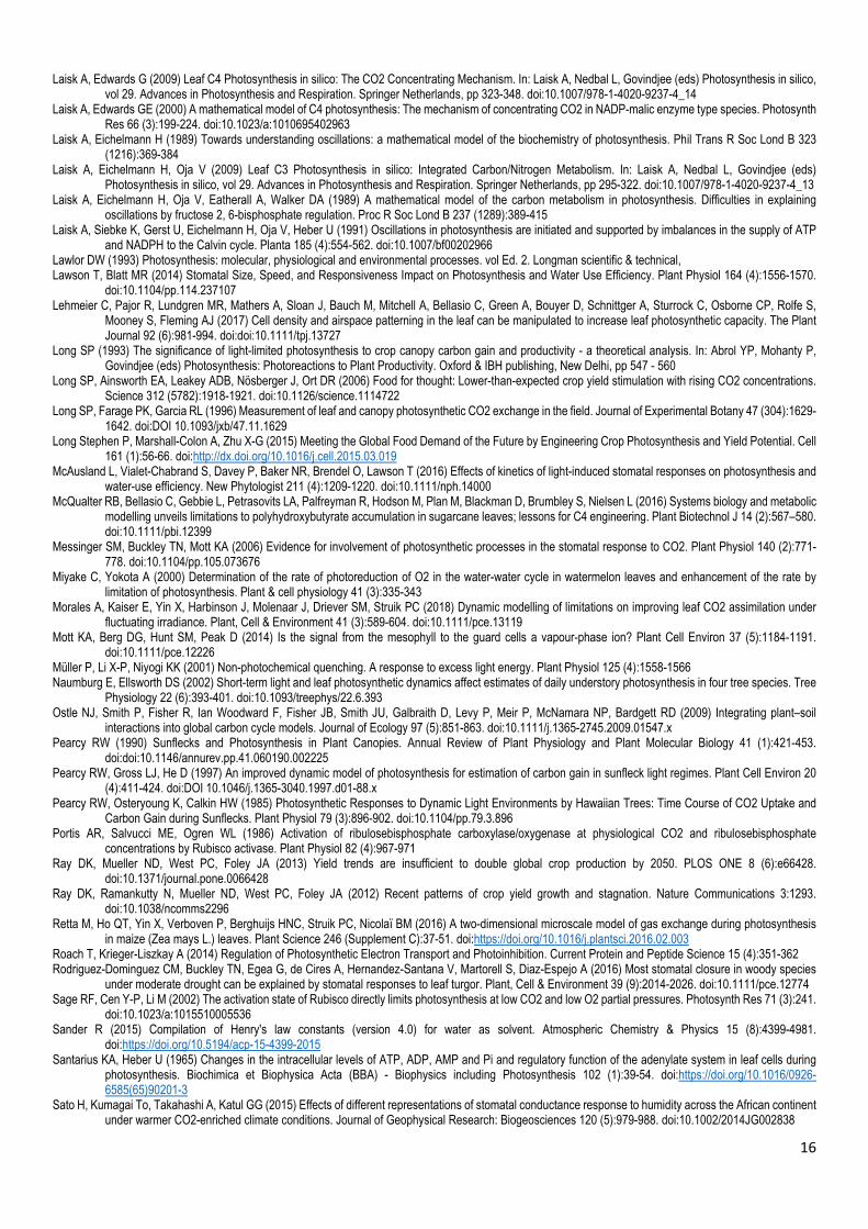
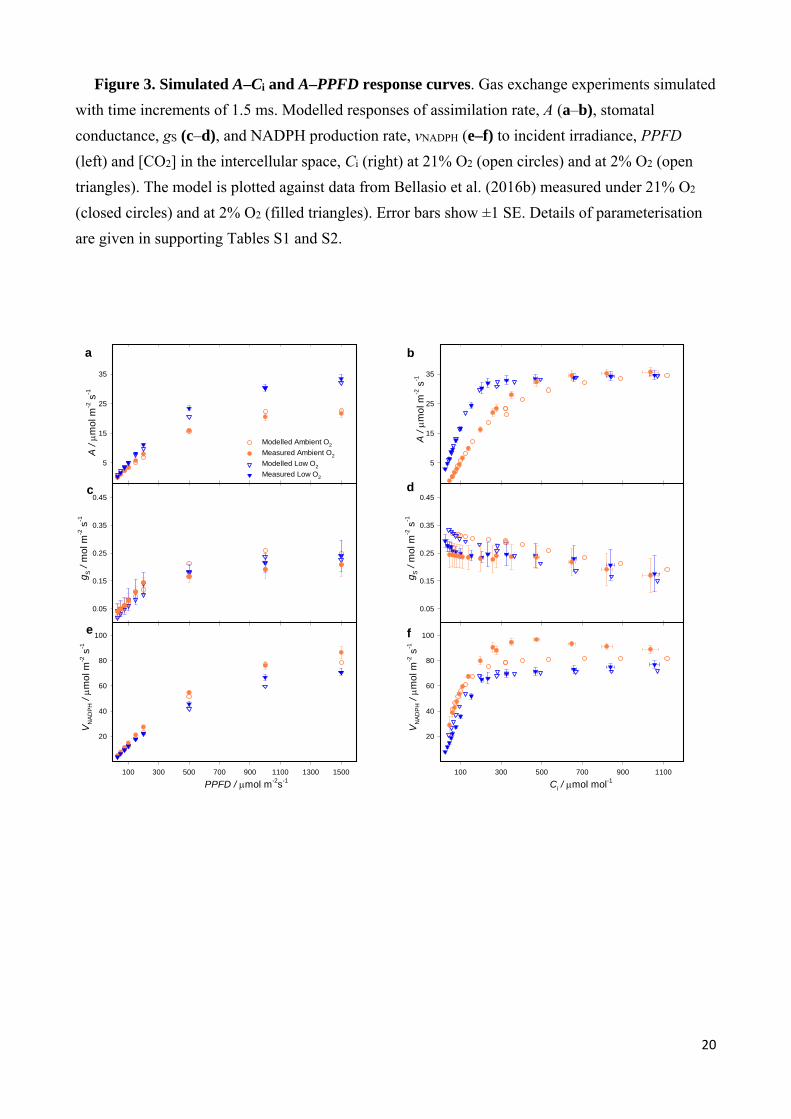
Figure 3 shows the modelled response of A, gs and vNADPH to variation in PPFD and Ca. Model 220

output corresponding to the values calculated for the last second of each PPFD or Ca step is 221

compared with Bellasio et al. (2016b) A–PPFD and A–Ci response curves measured in tobacco. 222

Overall, the agreement between observations and model output was high, even if the model was 223

parameterized with literature values not explicitly fitted to the data. For the A–PPFD curves, there 224

was no noteworthy deviation between modelled and observed values of A, gS or vNADPH (Figure 3, 225

left–hand panels). There was also overall good agreement between modelled and measured A–Ci 226

curves, though both A (Figure 3b) and vNADPH (Figure 3f) were underestimated at ambient O2 and Ci 227

> 300 µmol mol-1, and gS was slightly overestimated at low Ca (Figure 3d). Further analysis 228

revealed that under these conditions, modelled A was relatively unresponsive to individual increases 229

in relevant flow rates including JATP and JNADPH synthesis, RuP phosphorylation and VC. This 230

suggests complex, concurrent regulation of light and dark reactions that require further exploration. 231

2. Steady state concentration of photosynthetic metabolites 232

 

8  

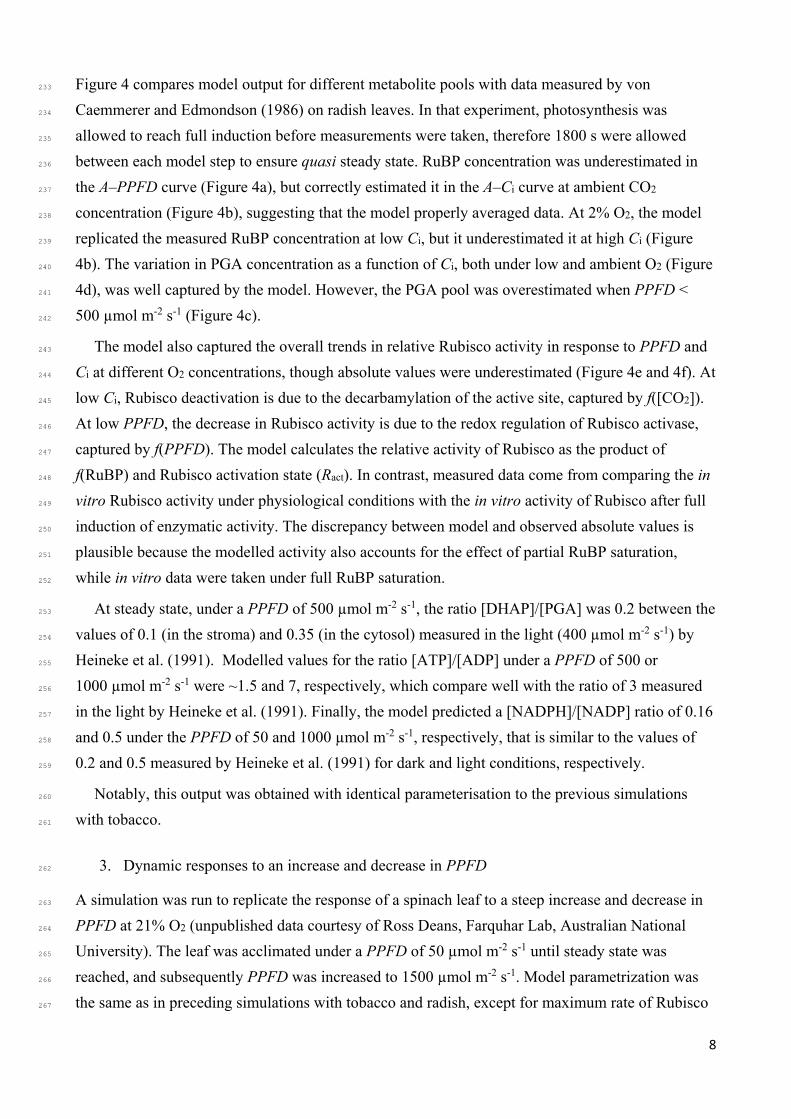
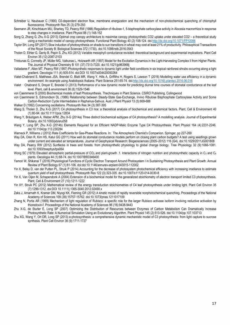
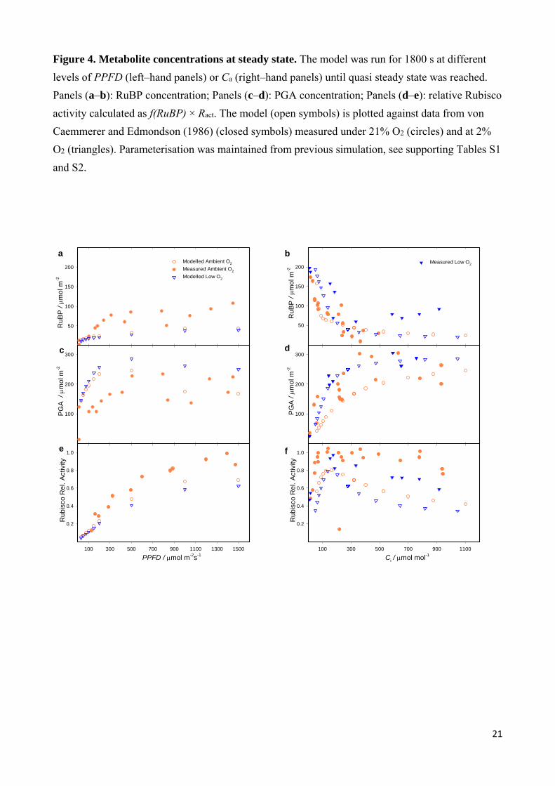
Figure 4 compares model output for different metabolite pools with data measured by von 233

Caemmerer and Edmondson (1986) on radish leaves. In that experiment, photosynthesis was 234

allowed to reach full induction before measurements were taken, therefore 1800 s were allowed 235

between each model step to ensure quasi steady state. RuBP concentration was underestimated in 236

the A–PPFD curve (Figure 4a), but correctly estimated it in the A–Ci curve at ambient CO2 237

concentration (Figure 4b), suggesting that the model properly averaged data. At 2% O2, the model 238

replicated the measured RuBP concentration at low Ci, but it underestimated it at high Ci (Figure 239

4b). The variation in PGA concentration as a function of Ci, both under low and ambient O2 (Figure 240

4d), was well captured by the model. However, the PGA pool was overestimated when PPFD < 241

500 µmol m-2 s-1 (Figure 4c). 242

The model also captured the overall trends in relative Rubisco activity in response to PPFD and 243

Ci at different O2 concentrations, though absolute values were underestimated (Figure 4e and 4f). At 244

low Ci, Rubisco deactivation is due to the decarbamylation of the active site, captured by f([CO2]). 245

At low PPFD, the decrease in Rubisco activity is due to the redox regulation of Rubisco activase, 246

captured by f(PPFD). The model calculates the relative activity of Rubisco as the product of 247

f(RuBP) and Rubisco activation state (Ract). In contrast, measured data come from comparing the in 248

vitro Rubisco activity under physiological conditions with the in vitro activity of Rubisco after full 249

induction of enzymatic activity. The discrepancy between model and observed absolute values is 250

plausible because the modelled activity also accounts for the effect of partial RuBP saturation, 251

while in vitro data were taken under full RuBP saturation. 252

At steady state, under a PPFD of 500 µmol m-2 s-1, the ratio [DHAP]/[PGA] was 0.2 between the 253

values of 0.1 (in the stroma) and 0.35 (in the cytosol) measured in the light (400 µmol m-2 s-1) by 254

Heineke et al. (1991). Modelled values for the ratio [ATP]/[ADP] under a PPFD of 500 or 255

1000 µmol m-2 s-1 were ~1.5 and 7, respectively, which compare well with the ratio of 3 measured 256

in the light by Heineke et al. (1991). Finally, the model predicted a [NADPH]/[NADP] ratio of 0.16 257

and 0.5 under the PPFD of 50 and 1000 µmol m-2 s-1, respectively, that is similar to the values of 258

0.2 and 0.5 measured by Heineke et al. (1991) for dark and light conditions, respectively. 259

Notably, this output was obtained with identical parameterisation to the previous simulations 260

with tobacco. 261

3. Dynamic responses to an increase and decrease in PPFD 262

A simulation was run to replicate the response of a spinach leaf to a steep increase and decrease in 263

PPFD at 21% O2 (unpublished data courtesy of Ross Deans, Farquhar Lab, Australian National 264

University). The leaf was acclimated under a PPFD of 50 µmol m-2 s-1 until steady state was 265

reached, and subsequently PPFD was increased to 1500 µmol m-2 s-1. Model parametrization was 266

the same as in preceding simulations with tobacco and radish, except for maximum rate of Rubisco 267

 

9  

carboxylation (VC MAX) and the speed of stomatal opening. Simulated dynamic responses of A and 268

gS corresponded closely with the measured data (Figure 5a and 5c). After the steep increase in 269

PPFD, ATP and NADPH production rates (Figure 5a), the Rubisco activation state (Figure 5b), and 270

ATP and DHAP concentrations (plotted as relative to the total pool of adenilates in Figure 5g) 271

followed a hyperbolic increase. ATP production increased faster than Rubisco activation state, 272

which resulted in an initial decrease in [PGA], a fast increase in [RuBP] and a subsequently sharp 273

decrease in [Pi] (Figure 5e). After ~150s, there was a continuous smooth decrease in f(RuBP), 274

resulting from the combination of increasing [PGA] and decreasing [RuBP] (Figure 5c). 275

Decreasing PPFD from 1500 µmol m-2 s-1 to 50 µmol m-2 s-1 resulted in a sharp initial reduction 276

in modelled A, followed by a hyperbolic increase to a new steady state value (Figure 5b). The 277

steady state modelled A slightly underestimated the measured rate (Figure 5b). A similar pattern 278

was followed by f(RuBP) (Figure 5 d) and [ATP] (Figure 5h), although they reached steady state 279

faster and slower than A, respectively. The ATP and NADPH production rates (Figure 5b) and 280

[NADPH] (Figure 5h) reached steady state almost immediately after an initial spike. The model 281

closely resembled the measured slow decrease in gS (Figure 5 d). The response of Rubisco 282

activation state (Figure 5d) was similar, although faster, than the observed trend in gs. [PGA] 283

sharply increased in the initial seconds after light reduction, and then decreased to a new steady 284

state value where [Pi] was higher than the initial value at high PPDF (Figure 5f). The initial sharp 285

increase in [PGA] was possible due to a high Rubisco activation state. This depleted the pool of 286

RuBP, which could not be regenerated because of insufficient light. The trend in [DHAP] was 287

comparable to the simulations of Laisk et al. (1989) [Figure 11 in Laisk et al. (1989)]. In contrast to 288

this model, Laisk et al. (1989) model predicted that [ATP], [Pi] and intermediates of the RPP cycle 289

had smooth transitions to steady state after perturbation without local maxima or minima. My 290

simulations are perhaps more realistic as they resemble measurements of [Pi] and [ATP] by 291

Santarius and Heber (1965), although with slower kinetics. 292

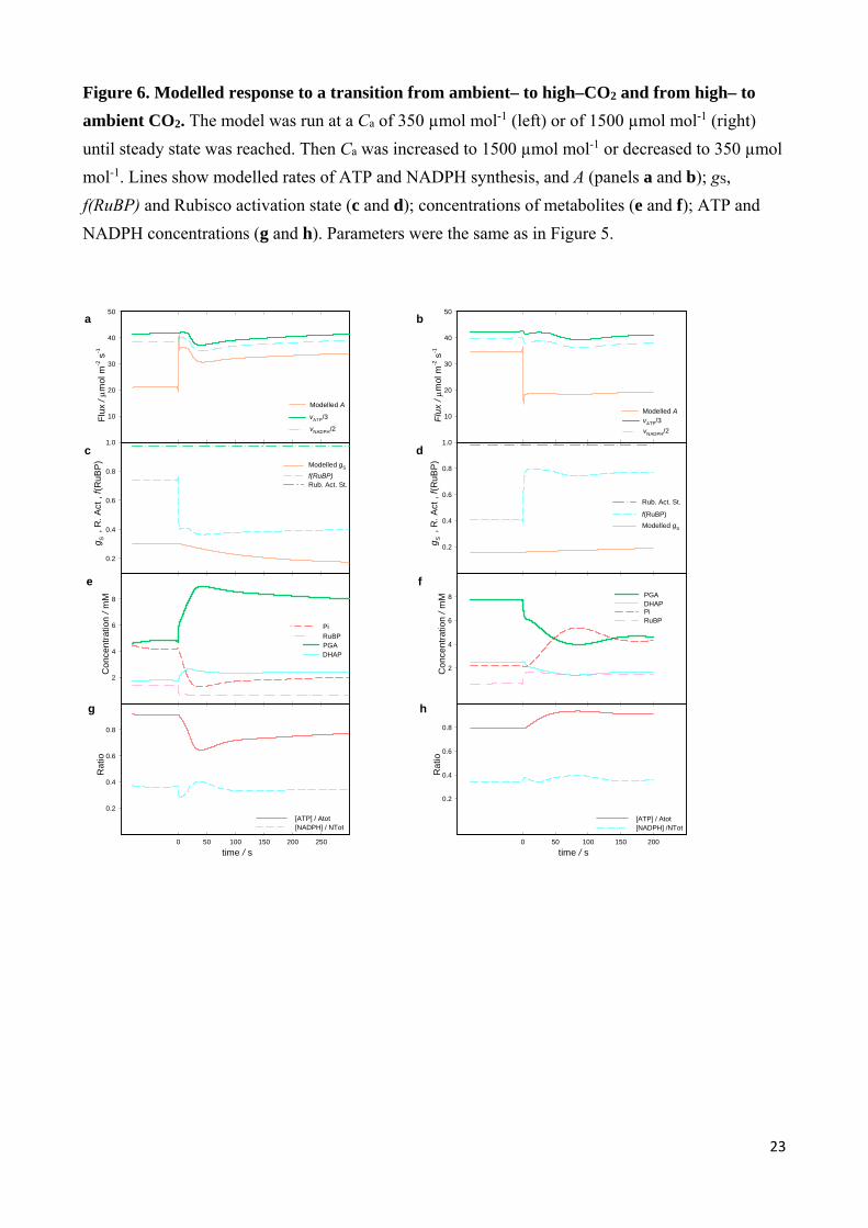
4. Dynamic responses to an increase and decrease in Ca 293

Model predictions for a steep increase (from 350 to 1500 µmol mol-1) or decrease (from 1500 to 294

350 µmol mol-1) in Ca were compared with data by Laisk et al. (1991). CS was timed with a first 295

order exponential delay function analogous to Eqn 41 with a time constant of 35 s. After the sudden 296

increase in Ca, A increased above 40 µmol m-2 s-1 for ~1s, which I attribute to the dissolution of CO2 297

into the leaf, then stabilised ~36 µmol m-2 s-1 for ~30s, which I attribute to the carboxylation of the 298

pool of phosphorylated metabolites. Finally A reached a minimum (Figure 6a) coincident with a 299

minimum in [Pi] (Figure 6e), vATP (Figure 6a) and [ATP] (Figure 6g). After these three phases, all 300

modelled quantities approached steady state smoothly. 301

After a steep decrease in Ca (Figure 6 b, d, f, g), A decreased for ~1s below the steady state value 302

before the perturbation, which can be explained by the stripping of dissolved CO2 out of the leaf. 303

 

10  

Subsequently A smoothly approached a new steady state value. The [PGA] reached a minimum 304

after ~80 s, which determined a maximum in [Pi] and a consequent maximum in vATP and [ATP]. 305

Overall, the model captured the dependence of A on Pi dynamics, which underpins the so–called 306

‘photosynthetic oscillations’ (Walker 1992). Further, modelled vATP (which is a function of the 307

reciprocal of leaf fluorescence) replicated the pattern of fluorescence shown by the simulations of 308

Laisk and Eichelmann (1989) [their Figure 5]. However, neither the model of Laisk and Eichelmann 309

(1989) nor mine captured the measured response of A beyond 30 s of induction, consisting of a very 310

deep trough in A lasting 10–20 s, followed by 4–5 dampened oscillations with a period of ~60 s 311

leading to a new steady state. 312

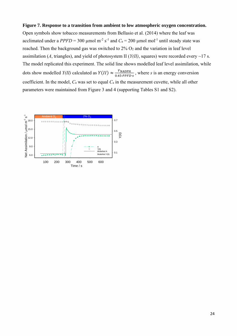
5. Dynamic responses to a decrease in atmospheric O2 concentration 313

A simulation was run to replicate the experiment of Bellasio et al. (2014), which involved assessing 314

the response of A and Y(II) to a decrease in [O2] in a tobacco leaf. The model accurately captured A 315

and Y(II) at steady state before and after the reduction in [O2]. The dynamic response of Y(II) was 316

also closely reproduced (Figure 7). However, modelled A failed to capture the initial spike 317

measured in A immediately after the reduction in [O2], which may be a measurement artefact that 318

originated during adjustments of the infrared gas analyser. 319

Discussion 320

A newly derived process–based stock–and–flow biochemical model of photosynthesis was 321

coupled to a dynamic hydro–mechanical model of stomatal behaviour. The new photosynthesis 322

model features time–explicit constraints on JATP, gS and Rubisco activation state. Steady state 323

metabolite concentrations are determined by environmental drivers and the kinetic parameters of 324

enzymes, but not by initial metabolite concentrations. The coupled model achieved a stable and 325

realistic rate of light–saturated A. After a perturbation in an environmental driver (e.g. PPFD), the 326

model was able to regain a specific steady state. The model successfully replicated gas exchange 327

experiments, including A–Ci and A–PPDF curves, and transient responses to steep changes in [O2], 328

Ca, and PPDF. 329

Simplifying assumptions 330

The mathematical description of dark reactions was simplified from Zhu et al. (2007) by reducing 331

the number of metabolites and reactions simulated, and removing some of the feedback loops. 332

Offloading of the RPP cycle to photosynthetic sinks was simplified into a single process called 333

carbohydrate synthesis (CS). Additionally, the reactions of the photorespiratory cycle were assumed 334

non–limiting. Additional feedbacks from sedoheptulose–1,7–bisphosphatase (SBPase) and 335

fructose–bisphosphate (FBP) (Wang et al. (2014b) were not included in the model. Feedbacks 336

characterised in vivo involve redox regulation [e.g. Zhang and Portis (1999)]. However, in the 337

 

11  

model, the dynamics of PGA depend solely on the equilibrium between its formation by Rubisco 338

and reduction. This approach was able to reproduce the response of PGA to PPDF observed by von 339

Caemmerer and Edmonson (1986) (Figure 4c). The pool of phosphorylated metabolites includes 340

PGA, DHAP RuP and RuBP. Additional pools of sugar phosphates were added in pilot simulations, 341

but for simplicity, were not included in the final model, nor was the activity of the malate shuttle 342

(Foyer et al. 1992). 343

Dynamic simulation of electron transporters can be computationally demanding (Zaks et al. 344

2012), therefore the flows associated with light reactions were described with classical equations, in 345

line with Wang et al. (2014a). This simplification implies that responses are instantaneous, which is 346

physiologically plausible because the speed of light reactions is higher than that of dark reactions 347

(Trinkunas et al. 1997). The model also ignored chloroplast movements, which have been shown to 348

dynamically vary in some species (Davis et al. 2011; Morales et al. 2018). Respiration was assumed 349

to be supplied by new assimilates (3–phosphoglyceric acid, PGA) following the original 350

formulation of Bellasio and Griffiths (2014) and subsequent developments (McQualter et al. 2016; 351

Bellasio 2017). The ATP and NADH produced during respiration were neglected because they are 352

likely to be consumed by basal metabolism. Although CS was made partially reversible (Eqn 28), a 353

calibration of metabolite replenishment in the dark is required before the model can be used for long 354

simulations around or below light– or CO2–compensation points. For further details on 355

assumptions, see Bellasio et al. (2017) and Bellasio (2017). 356

Comparison with other models 357

The model presented here characterises biochemical processes more comprehensively than 358

preceding models (Pearcy et al. 1997; Gross et al. 1991; Gross 1982) that featured 359

phenomenological pseudoreactions (Morales et al. 2018) not mechanistically linked to enzyme 360

activity. Additionally, my model is simpler, freely available, and therefore more readily applicable 361

than earlier models (Wang et al. 2014b; Zhu et al. 2013; Zhu et al. 2007; Laisk et al. 2009; Laisk 362

and Edwards 2009; Laisk and Edwards 2000; Laisk and Eichelmann 1989). Like the models of 363

Wang et al. (2017) and Morales et al. (2018), my model also responds to PPFD and external CO2 364

concentration, even at limiting levels. Importantly, in my model, light reactions can respond to 365

transitions in atmospheric [O2] (Figure 6). In addition to linking Rubisco activation to PPFD 366

(mediated by rubisco activase), a feature that some other models encompass, a distinctive feature of 367

my model is including a description of Rubisco inactivation at low [CO2] (mediated by 368

decarbamylation). I made both these drivers time–dependent with empirical functions. Lastly, and 369

uniquely, my model includes the process–based description of stomatal responses to a range of 370

environmental drivers such as humidity and soil water availability. 371

There are two main differences between the dynamic photosynthesis model of Morales et al. 372

(2018) and the model described here. In the model by Morales et al. (2018), there are two dynamic 373

 

12  

processes: Rubisco and a pseudo–reaction associated to RuBP regeneration. In my model, there are 374

nine dynamic reactions in the dark phase, which are mechanistically dependent on the concentration 375

of 12 metabolites. In Morales et al. (2018), light reactions are simulated dynamically with explicit 376

description of quenching phenomena. In my model, there is full integration between dark reactions 377

and the electron transport chain, including: feedbacks at the level of cyclic electron flow 378

engagement; at the link between O2 concentration and electron flow through the glutathione –379

ascorbate peroxidase (APX) cycle; and at the level of Y(II). The latter is dependent on [ATP], 380

[NADPH] and [Pi] mediated by the kinetics of ATP synthesis. 381

In most dynamic and steady state models, feedbacks are accounted for with a discontinuous 382

function selecting between the ‘minimum of’ two or more quantities. For instance, Busch and Sage 383

(2017) calculated A by selecting between three limiting factors: light, enzyme capacity, or triose 384

phosphate availability. In Wang et al. (2014a) and preceding models, the calculation of VC is 385

underpinned by the selection between RuBP or CO2 limitations. In my model, all biochemical 386

feedbacks operate continuously. The transition from light– to enzyme–limitation is smooth, 387

pivoting around the poise between regeneration and use of RuBP. This poise is captured by a 388

quadratic function, f(RuBP), which depends on the concentration of RuBP relative to the 389

concentration of Rubisco catalytic sites. This function was originally developed by Farquhar et al. 390

(1980) (VC/WC in their notation, representing the actual, relative to the RuBP–saturated, rate of 391

carboxylation), but it has rarely been implemented in its full quadratic form. The transition to TPU 392

limitation is also smooth but in this case, is underpinned by a decreasing amount of Pi liberated by 393

CS, thereby reducing [Pi] thats feedbacks directly on vATP and indirectly over Y(II). Under TPU 394

limitation, assimilation is controlled by VMAX CS. 395

Simulation processing time 396

On a standard desktop or laptop computer (~4 GB of RAM and ~2 GHz CPU speed), the model 397

cycles at ~1000 Hz, with the actual time taken for a simulation run depending on the integration 398

time step. The model is ‘stiff’, therefore the steplength is constrained by stability requirements, 399

rather than those of accuracy. The model becomes unstable when the fluxes accrued over the time 400

step become comparable with the corresponding stocks. Of course, the fastest reactions such as 401

those involving CO2 diffusion and hydration are the most affected. If carbonic anhydrase (CA) is 402

included in calculations, the model is unstable at time steps greater than 0.5 ms. Using an 403

integration step of 0.3 ms, it takes ~35 s of computation time to simulate 10 s transition, and 42 404

hours to simulate a 12–hr photoperiod. 405

Stability can be improved by ignoring CA activity, which makes the model stable for time steps 406

shorter than 2 ms. CA may be relevant at timescales shorter than 0.1 s and was included in the 407

model because it has been deemed important in a number of recent studies [e.g. (Ho et al. 2015)]; 408

 

13  

however, excluding CA did not change the model outputs presented here. Using a step of 1.5 ms, it 409

takes ~7 s of processing time to simulate 10 s and 8.4 hours to simulate a 12–hr photoperiod. 410

Stability can also be ameliorated by incrementing the stocks. In this model, the residual leaf 411

volume, occupied by cell walls and apoplastic solution, is all assumed to be intercellular air. A 412

higher volume allows better model stability, because the flux of incoming CO2 is buffered by a 413

larger pool of air. Thickness and porosity may need to be adjusted for specific applications, for 414

instance, for simulating airspace patterning manipulation (Lehmeier et al. 2017). Improvements in 415

speed can also be achieved by assuming that CO2 in the liquid phase is in equilibrium with 416

bicarbonate, forming a common stock. 417

The Excel® workbook incorporates a selection feature allowing the user to include or 418

exclude these simplifications and automatically amends the calculations according to the selection. 419

Ignoring CA and assuming a common pool with bicarbonate, the maximum time step scales with 420

the reciprocal of gS (determining the entrant flow of CO2) and the model can be used reliably with a 421

5 ms resolution under a range of conditions. 422

Future developments 423

I am currently working on simulating photosynthetic oscillations. This involves adding 424

complexity to the description of CS, new feedback loops, and perhaps allowing multiple timings for 425

signalling functions. Subsequently, I plan to model the triose phosphate utilisation to reproduce the 426

patterns experimentally described by Busch et al. (2017). In the long term, this model will form the 427

core of an emerging C4 model, encompassing all C3 features presented here plus a dynamic 428

description of C4 metabolite diffusion. 429

In my model, stomatal conductance follows first–order kinetics, but it could be adapted to allow 430

for the sigmoidal kinetics used in other studies (Kirschbaum et al. 1997; Vialet‐Chabrand et al. 431

2013). Another development for the model is the mechanistic implementation of a simplified, 432

dynamic and integrated electron transport chain building on the basis of previous work (Zaks et al. 433

2012; Laisk and Eichelmann 1989; Zhu et al. 2013; Morales et al. 2018), but including some of the 434

continuous feedbacks present in this model and others (Joliot and Johnson 2011; Roach and 435

Krieger-Liszkay 2014; Foyer et al. 2012). 436

Shorter processing time could be achieved if all calculations were performed directly using the 437

Excel®–embedded VBA® (Visual Basic for Applications, or another suitable software). This would 438

avoid the need for VBA® and Excel® to interact at every cycle. I choose to keep all the equations in 439

the Excel® workbook to maximise transparency, and to allow straightforward model modification 440

and parameterisation without the necessity of modifying the code, which only iterates results. 441

Further gains in processing speed could be achieved by substituting the simple Euler integration, 442

 

14  

whereby the model is calculated at each time increment, with more sophisticated calculus involving 443

stiff solvers and parallel integration with a range of suitable time steps. 444

Many of the parameters used to model photosynthesis are temperature dependent. Given the 445

large number of parameters and the difficulty in experimentally resolving the dependency of 446

individual quantities, I opted for not including temperature at this stage, but it should be addressed 447

in the future. 448

Conclusion 449

Models are descriptions of natural systems that trade–off comprehensiveness with the simplicity 450

and ease of use. Traditional steady–state models are simple but inherently unsuitable for assessing 451

rapid responses of photosynthesis to environmental drivers. Dynamic models are more complex, but 452

are needed to study rapid responses to environmental perturbation. I derived a dynamic process–453

based photosynthetic model for C3 leaves simplifying wherever possible while integrating and 454

expanding the functionalities of recently published dynamic models. In particular, my model 455

combines a hydromechanical model of stomatal behaviour with dynamic descriptions of dark and 456

light reactions. The model is presented in a transparent format and can be run as a freely 457

downloadable, stand–alone workbook in Microsoft® Excel®. The model successfully replicated 458

complete gas exchange experiments featuring both short lag times and full photosynthetic 459

acclimation, as well as dynamic transitions between light, CO2 and oxygen levels. The model has 460

the potential to supersede steady state models for detailed or time–dependent ecophysiological 461

studies and I encourage its use for basic research in photosynthesis. Steady–state models will 462

remain useful for larger scale simulations. 463

Availability 464

The model, coded in Microsoft® Excel®, is freely available from the Supplementary Information 465

associated with the online version of this paper. A video tutorial is available on Youtube at the 466

following link: (to be added when available). 467

 

 

15  

References

Allen WA, Richardson AJ (1968) Interaction of Light with a Plant Canopy. J Opt Soc Am 58 (8):1023-1028. doi:Doi 10.1364/Josa.58.001023 Beerling DJ (2015) Gas valves, forests and global change: a commentary on Jarvis (1976) ‘The interpretation of the variations in leaf water potential and stomatal

conductance found in canopies in the field’. Philosophical Transactions of the Royal Society B: Biological Sciences 370 (1666). doi:10.1098/rstb.2014.0311

Bellasio C (2017) A generalised stoichiometric model of C3, C2, C2+C4, and C4 photosynthetic metabolism. Journal of Experimental Botany 68 (2):269-282. doi:doi: 10.1093/jxb/erw303

Bellasio C, Beerling DJ, Griffiths H (2016a) Deriving C4 photosynthetic parameters from combined gas exchange and chlorophyll fluorescence using an Excel tool: theory and practice. Plant, Cell & Environment 39 (6):1164-1179. doi:10.1111/pce.12626

Bellasio C, Beerling DJ, Griffiths H (2016b) An Excel tool for deriving key photosynthetic parameters from combined gas exchange and chlorophyll fluorescence: theory and practice. Plant Cell Environ 39 (6):1180–1197. doi:DOI: 10.1111/pce.12560

Bellasio C, Burgess SJ, Griffiths H, Hibberd JM (2014) A high throughput gas exchange screen for determining rates of photorespiration or regulation of C4 activity. Journal of Experimental Botany 65 (13):3769-3779. doi:10.1093/jxb/eru238

Bellasio C, Griffiths H (2014) The operation of two decarboxylases (NADPME and PEPCK), transamination and partitioning of C4 metabolic processes between mesophyll and bundle sheath cells allows light capture to be balanced for the maize C4 pathway. Plant Physiol 164:466-480. doi:DOI: 10.1111/pce.12194

Bellasio C, Quirk J, Buckley TN, Beerling D (2017) A dynamic hydro-mechanical and biochemical model of stomatal conductance for C4 photosynthesis. Plant Physiol. doi:10.1104/pp.17.00666

Berry JA, Beerling DJ, Franks PJ (2010) Stomata: key players in the earth system, past and present. Current Opinion in Plant Biology 13 (3):232-239. doi:https://doi.org/10.1016/j.pbi.2010.04.013

Bonan GB, Williams M, Fisher RA, Oleson KW (2014) Modeling stomatal conductance in the earth system: linking leaf water-use efficiency and water transport along the soil–plant–atmosphere continuum. Geosci Model Dev 7 (5):2193-2222. doi:10.5194/gmd-7-2193-2014

Buckley TN (2017) Modeling stomatal conductance. Plant Physiol DOI:10.1104/pp.16.01772. doi:10.1104/pp.16.01772 Buckley TN, Mott KA, Farquhar GD (2003) A hydromechanical and biochemical model of stomatal conductance. Plant, Cell & Environment 26 (10):1767-1785.

doi:10.1046/j.1365-3040.2003.01094.x Busch FA (2014) Opinion: The red-light response of stomatal movement is sensed by the redox state of the photosynthetic electron transport chain. Photosynth

Res 119 (1-2):131-140. doi:10.1007/s11120-013-9805-6 Busch FA, Sage RF (2017) The sensitivity of photosynthesis to O2 and CO2 concentration identifies strong Rubisco control above the thermal optimum. New

Phytologist 213 (3):1036-1051. doi:10.1111/nph.14258 Busch FA, Sage RF, Farquhar GD (2017) Plants increase CO2 uptake by assimilating nitrogen via the photorespiratory pathway. Nature Plants DOI:

10.1038/s41477-017-0065-x. doi:10.1038/s41477-017-0065-x Damour G, Simonneau T, Cochard H, Urban L (2010) An overview of models of stomatal conductance at the leaf level. Plant, Cell & Environment 33 (9):1419-

1438. doi:10.1111/j.1365-3040.2010.02181.x Davis PA, Caylor S, Whippo CW, Hangarter RP (2011) Changes in leaf optical properties associated with light‐dependent chloroplast movements. Plant, cell &

environment 34 (12):2047-2059 Driever SM, Simkin AJ, Alotaibi S, Fisk SJ, Madgwick PJ, Sparks CA, Jones HD, Lawson T, Parry MAJ, Raines CA (2017) Increased SBPase activity improves

photosynthesis and grain yield in wheat grown in greenhouse conditions. Philosophical Transactions of the Royal Society B: Biological Sciences 372 (1730). doi:10.1098/rstb.2016.0384

Farquhar G, Wong S (1984) An empirical model of stomatal conductance. Functional Plant Biology 11 (3):191-210. doi:10.1071/PP9840191 Farquhar GD, von Caemmerer S, Berry JA (1980) A biochemical-model of photosynthetic CO2 assimilation in leaves of C3 species. Planta 149 (1):78-90.

doi:10.1007/bf00386231 Foyer CH, Lelandais M, Harbinson J (1992) Control of the quantum efficiencies of photosystems I and II, electron flow, and enzyme activation following dark-to-

light transitions in pea leaves: relationship between NADP/NADPH ratios and NADP-malate dehydrogenase activation state. Plant Physiol 99 (3):979-986

Foyer CH, Neukermans J, Queval G, Noctor G, Harbinson J (2012) Photosynthetic control of electron transport and the regulation of gene expression. Journal of Experimental Botany 63 (4):1637-1661. doi:10.1093/jxb/ers013

Gross LJ (1982) Photosynthetic dynamics in varying light environments: a model and its application to whole leaf carbon gain. Ecology 63 (1):84-93 Gross LJ, Kirschbaum MUF, Pearcy RW (1991) A Dynamic-Model of Photosynthesis in Varying Light Taking Account of Stomatal Conductance, C3-Cycle

Intermediates, Photorespiration and Rubisco Activation. Plant Cell Environ 14 (9):881-893. doi:DOI 10.1111/j.1365-3040.1991.tb00957.x Heineke D, Riens B, Grosse H, Hoferichter P, Peter U, Flügge U-I, Heldt HW (1991) Redox transfer across the inner chloroplast envelope membrane. Plant

Physiol 95 (4):1131-1137 Hendrey G, Long S, McKee I, Baker N (1997) Can photosynthesis respond to short-term fluctuations in atmospheric carbon dioxide? Photosynth Res 51 (3):179-

184 Ho QT, Berghuijs HNC, WattÉ R, Verboven P, Herremans ELS, Yin X, Retta MA, Aernouts BEN, Saeys W, Helfen L, Farquhar GD, Struik PC, NicolaÏ BM (2015)

Three-dimensional microscale modelling of CO2 transport and light propagation in tomato leaves enlightens photosynthesis. Plant, Cell & Environment:n/a-n/a. doi:10.1111/pce.12590

Ishikawa N, Takabayashi A, Sato F, Endo T (2016) Accumulation of the components of cyclic electron flow around photosystem I in C4 plants, with respect to the requirements for ATP. Photosynth Res:1-17. doi:10.1007/s11120-016-0251-0

Joliot P, Johnson GN (2011) Regulation of cyclic and linear electron flow in higher plants. Proceedings of the National Academy of Sciences 108 (32):13317-13322. doi:10.1073/pnas.1110189108

Kaiser E, Morales A, Harbinson J, Kromdijk J, Heuvelink E, Marcelis LFM (2014) Dynamic photosynthesis in different environmental conditions. Journal of Experimental Botany. doi:10.1093/jxb/eru406

Kirschbaum M, Küppers M, Schneider H, Giersch C, Noe S (1997) Modelling photosynthesis in fluctuating light with inclusion of stomatal conductance, biochemical activation and pools of key photosynthetic intermediates. Planta 204 (1):16-26

Kramer DM, Evans JR (2011) The Importance of Energy Balance in Improving Photosynthetic Productivity. Plant Physiol 155 (1):70-78. doi:DOI 10.1104/pp.110.166652

Kromdijk J, Głowacka K, Leonelli L, Gabilly ST, Iwai M, Niyogi KK, Long SP (2016) Improving photosynthesis and crop productivity by accelerating recovery from photoprotection. Science 354 (6314):857-861. doi:10.1126/science.aai8878

 

16  

Laisk A, Edwards G (2009) Leaf C4 Photosynthesis in silico: The CO2 Concentrating Mechanism. In: Laisk A, Nedbal L, Govindjee (eds) Photosynthesis in silico, vol 29. Advances in Photosynthesis and Respiration. Springer Netherlands, pp 323-348. doi:10.1007/978-1-4020-9237-4_14

Laisk A, Edwards GE (2000) A mathematical model of C4 photosynthesis: The mechanism of concentrating CO2 in NADP-malic enzyme type species. Photosynth Res 66 (3):199-224. doi:10.1023/a:1010695402963

Laisk A, Eichelmann H (1989) Towards understanding oscillations: a mathematical model of the biochemistry of photosynthesis. Phil Trans R Soc Lond B 323 (1216):369-384

Laisk A, Eichelmann H, Oja V (2009) Leaf C3 Photosynthesis in silico: Integrated Carbon/Nitrogen Metabolism. In: Laisk A, Nedbal L, Govindjee (eds) Photosynthesis in silico, vol 29. Advances in Photosynthesis and Respiration. Springer Netherlands, pp 295-322. doi:10.1007/978-1-4020-9237-4_13

Laisk A, Eichelmann H, Oja V, Eatherall A, Walker DA (1989) A mathematical model of the carbon metabolism in photosynthesis. Difficulties in explaining oscillations by fructose 2, 6-bisphosphate regulation. Proc R Soc Lond B 237 (1289):389-415

Laisk A, Siebke K, Gerst U, Eichelmann H, Oja V, Heber U (1991) Oscillations in photosynthesis are initiated and supported by imbalances in the supply of ATP and NADPH to the Calvin cycle. Planta 185 (4):554-562. doi:10.1007/bf00202966

Lawlor DW (1993) Photosynthesis: molecular, physiological and environmental processes. vol Ed. 2. Longman scientific & technical, Lawson T, Blatt MR (2014) Stomatal Size, Speed, and Responsiveness Impact on Photosynthesis and Water Use Efficiency. Plant Physiol 164 (4):1556-1570.

doi:10.1104/pp.114.237107 Lehmeier C, Pajor R, Lundgren MR, Mathers A, Sloan J, Bauch M, Mitchell A, Bellasio C, Green A, Bouyer D, Schnittger A, Sturrock C, Osborne CP, Rolfe S,

Mooney S, Fleming AJ (2017) Cell density and airspace patterning in the leaf can be manipulated to increase leaf photosynthetic capacity. The Plant Journal 92 (6):981-994. doi:doi:10.1111/tpj.13727

Long SP (1993) The significance of light-limited photosynthesis to crop canopy carbon gain and productivity - a theoretical analysis. In: Abrol YP, Mohanty P, Govindjee (eds) Photosynthesis: Photoreactions to Plant Productivity. Oxford & IBH publishing, New Delhi, pp 547 - 560

Long SP, Ainsworth EA, Leakey ADB, Nösberger J, Ort DR (2006) Food for thought: Lower-than-expected crop yield stimulation with rising CO2 concentrations. Science 312 (5782):1918-1921. doi:10.1126/science.1114722

Long SP, Farage PK, Garcia RL (1996) Measurement of leaf and canopy photosynthetic CO2 exchange in the field. Journal of Experimental Botany 47 (304):1629-1642. doi:DOI 10.1093/jxb/47.11.1629

Long Stephen P, Marshall-Colon A, Zhu X-G (2015) Meeting the Global Food Demand of the Future by Engineering Crop Photosynthesis and Yield Potential. Cell 161 (1):56-66. doi:http://dx.doi.org/10.1016/j.cell.2015.03.019

McAusland L, Vialet-Chabrand S, Davey P, Baker NR, Brendel O, Lawson T (2016) Effects of kinetics of light-induced stomatal responses on photosynthesis and water-use efficiency. New Phytologist 211 (4):1209-1220. doi:10.1111/nph.14000

McQualter RB, Bellasio C, Gebbie L, Petrasovits LA, Palfreyman R, Hodson M, Plan M, Blackman D, Brumbley S, Nielsen L (2016) Systems biology and metabolic modelling unveils limitations to polyhydroxybutyrate accumulation in sugarcane leaves; lessons for C4 engineering. Plant Biotechnol J 14 (2):567–580. doi:10.1111/pbi.12399

Messinger SM, Buckley TN, Mott KA (2006) Evidence for involvement of photosynthetic processes in the stomatal response to CO2. Plant Physiol 140 (2):771-778. doi:10.1104/pp.105.073676

Miyake C, Yokota A (2000) Determination of the rate of photoreduction of O2 in the water-water cycle in watermelon leaves and enhancement of the rate by limitation of photosynthesis. Plant & cell physiology 41 (3):335-343

Morales A, Kaiser E, Yin X, Harbinson J, Molenaar J, Driever SM, Struik PC (2018) Dynamic modelling of limitations on improving leaf CO2 assimilation under fluctuating irradiance. Plant, Cell & Environment 41 (3):589-604. doi:10.1111/pce.13119

Mott KA, Berg DG, Hunt SM, Peak D (2014) Is the signal from the mesophyll to the guard cells a vapour-phase ion? Plant Cell Environ 37 (5):1184-1191. doi:10.1111/pce.12226

Müller P, Li X-P, Niyogi KK (2001) Non-photochemical quenching. A response to excess light energy. Plant Physiol 125 (4):1558-1566 Naumburg E, Ellsworth DS (2002) Short-term light and leaf photosynthetic dynamics affect estimates of daily understory photosynthesis in four tree species. Tree

Physiology 22 (6):393-401. doi:10.1093/treephys/22.6.393 Ostle NJ, Smith P, Fisher R, Ian Woodward F, Fisher JB, Smith JU, Galbraith D, Levy P, Meir P, McNamara NP, Bardgett RD (2009) Integrating plant–soil

interactions into global carbon cycle models. Journal of Ecology 97 (5):851-863. doi:10.1111/j.1365-2745.2009.01547.x Pearcy RW (1990) Sunflecks and Photosynthesis in Plant Canopies. Annual Review of Plant Physiology and Plant Molecular Biology 41 (1):421-453.

doi:doi:10.1146/annurev.pp.41.060190.002225 Pearcy RW, Gross LJ, He D (1997) An improved dynamic model of photosynthesis for estimation of carbon gain in sunfleck light regimes. Plant Cell Environ 20

(4):411-424. doi:DOI 10.1046/j.1365-3040.1997.d01-88.x Pearcy RW, Osteryoung K, Calkin HW (1985) Photosynthetic Responses to Dynamic Light Environments by Hawaiian Trees: Time Course of CO2 Uptake and

Carbon Gain during Sunflecks. Plant Physiol 79 (3):896-902. doi:10.1104/pp.79.3.896 Portis AR, Salvucci ME, Ogren WL (1986) Activation of ribulosebisphosphate carboxylase/oxygenase at physiological CO2 and ribulosebisphosphate

concentrations by Rubisco activase. Plant Physiol 82 (4):967-971 Ray DK, Mueller ND, West PC, Foley JA (2013) Yield trends are insufficient to double global crop production by 2050. PLOS ONE 8 (6):e66428.

doi:10.1371/journal.pone.0066428 Ray DK, Ramankutty N, Mueller ND, West PC, Foley JA (2012) Recent patterns of crop yield growth and stagnation. Nature Communications 3:1293.

doi:10.1038/ncomms2296 Retta M, Ho QT, Yin X, Verboven P, Berghuijs HNC, Struik PC, Nicolaï BM (2016) A two-dimensional microscale model of gas exchange during photosynthesis

in maize (Zea mays L.) leaves. Plant Science 246 (Supplement C):37-51. doi:https://doi.org/10.1016/j.plantsci.2016.02.003 Roach T, Krieger-Liszkay A (2014) Regulation of Photosynthetic Electron Transport and Photoinhibition. Current Protein and Peptide Science 15 (4):351-362 Rodriguez-Dominguez CM, Buckley TN, Egea G, de Cires A, Hernandez-Santana V, Martorell S, Diaz-Espejo A (2016) Most stomatal closure in woody species

under moderate drought can be explained by stomatal responses to leaf turgor. Plant, Cell & Environment 39 (9):2014-2026. doi:10.1111/pce.12774 Sage RF, Cen Y-P, Li M (2002) The activation state of Rubisco directly limits photosynthesis at low CO2 and low O2 partial pressures. Photosynth Res 71 (3):241.

doi:10.1023/a:1015510005536 Sander R (2015) Compilation of Henry's law constants (version 4.0) for water as solvent. Atmospheric Chemistry & Physics 15 (8):4399-4981.

doi:https://doi.org/10.5194/acp-15-4399-2015 Santarius KA, Heber U (1965) Changes in the intracellular levels of ATP, ADP, AMP and Pi and regulatory function of the adenylate system in leaf cells during

photosynthesis. Biochimica et Biophysica Acta (BBA) - Biophysics including Photosynthesis 102 (1):39-54. doi:https://doi.org/10.1016/0926-6585(65)90201-3

Sato H, Kumagai To, Takahashi A, Katul GG (2015) Effects of different representations of stomatal conductance response to humidity across the African continent under warmer CO2-enriched climate conditions. Journal of Geophysical Research: Biogeosciences 120 (5):979-988. doi:10.1002/2014JG002838

 

17  

Schreiber U, Neubauer C (1990) O2-dependent electron flow, membrane energization and the mechanism of non-photochemical quenching of chlorophyll fluorescence. Photosynth Res 25 (3):279-293

Seemann JR, Kirschbaum MU, Sharkey TD, Pearcy RW (1988) Regulation of ribulose-1, 5-bisphosphate carboxylase activity in Alocasia macrorrhiza in response to step changes in irradiance. Plant Physiol 88 (1):148-152

Song Q, Zhang G, Zhu X-G (2013) Optimal crop canopy architecture to maximise canopy photosynthetic CO2 uptake under elevated CO2 – a theoretical study using a mechanistic model of canopy photosynthesis. Functional Plant Biology 40 (2):108-124. doi:http://dx.doi.org/10.1071/FP12056

Taylor SH, Long SP (2017) Slow induction of photosynthesis on shade to sun transitions in wheat may cost at least 21% of productivity. Philosophical Transactions of the Royal Society B: Biological Sciences 372 (1730). doi:10.1098/rstb.2016.0543

Tholen D, Ethier G, Genty B, Pepin S, Zhu XG (2012) Variable mesophyll conductance revisited: theoretical background and experimental implications. Plant Cell Environ 35 (12):2087-2103

Trinkunas G, Connelly JP, Müller MG, Valkunas L, Holzwarth AR (1997) Model for the Excitation Dynamics in the Light-Harvesting Complex II from Higher Plants. The Journal of Physical Chemistry B 101 (37):7313-7320. doi:10.1021/jp963968j

Valladares F, Allen MT, Pearcy RW (1997) Photosynthetic responses to dynamic light under field conditions in six tropical rainforest shrubs occurring along a light gradient. Oecologia 111 (4):505-514. doi:DOI 10.1007/s004420050264

Vialet-Chabrand S, Matthews JSA, Brendel O, Blatt MR, Wang Y, Hills A, Griffiths H, Rogers S, Lawson T (2016) Modelling water use efficiency in a dynamic environment: An example using Arabidopsis thaliana. Plant Science 251:65-74. doi:http://dx.doi.org/10.1016/j.plantsci.2016.06.016

Vialet‐Chabrand S, Dreyer E, Brendel O (2013) Performance of a new dynamic model for predicting diurnal time courses of stomatal conductance at the leaf level. Plant, cell & environment 36 (8):1529-1546

von Caemmerer S (2000) Biochemical models of leaf Photosynthesis. Thechniques in Plant Science. CSIRO Publishing, Collingwood von Caemmerer S, Edmondson DL (1986) Relationship between Steady-State Gas-Exchange, Invivo Ribulose Bisphosphate Carboxylase Activity and Some

Carbon-Reduction Cycle Intermediates in Raphanus-Sativus. Aust J Plant Physiol 13 (5):669-688 Walker D (1992) Concerning oscillations. Photosynth Res 34 (3):387-395 Wang S, Tholen D, Zhu X-G (2017) C4 photosynthesis in C3 rice: a theoretical analysis of biochemical and anatomical factors. Plant, Cell & Environment 40

(1):80-94. doi:10.1111/pce.12834 Wang Y, Bräutigam A, Weber APM, Zhu X-G (2014a) Three distinct biochemical subtypes of C4 photosynthesis? A modelling analysis. Journal of Experimental

Botany. doi:10.1093/jxb/eru058 Wang Y, Long SP, Zhu X-G (2014b) Elements Required for an Efficient NADP-Malic Enzyme Type C4 Photosynthesis. Plant Physiol 164 (4):2231-2246.

doi:10.1104/pp.113.230284 Warneck P, Williams J (2012) Rate Coefficients for Gas-Phase Reactions. In: The Atmospheric Chemist’s Companion. Springer, pp 227-269 Way DA, Oren R, Kim HS, Katul GG (2011) How well do stomatal conductance models perform on closing plant carbon budgets? A test using seedlings grown

under current and elevated air temperatures. Journal of Geophysical Research: Biogeosciences (2005–2012) 116 (G4). doi:10.1029/2011JG001808 Way DA, Pearcy RW (2012) Sunflecks in trees and forests: from photosynthetic physiology to global change biology. Tree Physiology 32 (9):1066-1081.

doi:10.1093/treephys/tps064 Wong SC (1979) Elevated atmospheric partial-pressure of CO2 and plant-growth .1. Interactions of nitrogen nutrition and photosynthetic capacity in C3 and C4

plants. Oecologia 44 (1):68-74. doi:10.1007/Bf00346400 Yamori W, Shikanai T (2016) Physiological Functions of Cyclic Electron Transport Around Photosystem I in Sustaining Photosynthesis and Plant Growth. Annual

Review of Plant Biology 67 (1):81-106. doi:doi:10.1146/annurev-arplant-043015-112002 Yin X, Belay D, van der Putten PL, Struik P (2014) Accounting for the decrease of photosystem photochemical efficiency with increasing irradiance to estimate

quantum yield of leaf photosynthesis. Photosynth Res 122 (3):323-335. doi:10.1007/s11120-014-0030-8 Yin X, Van Oijen M, Schapendonk A (2004) Extension of a biochemical model for the generalized stoichiometry of electron transport limited C3 photosynthesis.

Plant, Cell & Environment 27 (10):1211-1222 Yin XY, Struik PC (2012) Mathematical review of the energy transduction stoichiometries of C4 leaf photosynthesis under limiting light. Plant Cell Environ 35

(7):1299-1312. doi:DOI 10.1111/j.1365-3040.2012.02490.x Zaks J, Amarnath K, Kramer DM, Niyogi KK, Fleming GR (2012) A kinetic model of rapidly reversible nonphotochemical quenching. Proceedings of the National

Academy of Sciences 109 (39):15757-15762. doi:10.1073/pnas.1211017109 Zhang N, Portis AR (1999) Mechanism of light regulation of Rubisco: a specific role for the larger Rubisco activase isoform involving reductive activation by

thioredoxin-f. Proceedings of the National Academy of Sciences 96 (16):9438-9443 Zhu X-G, de Sturler E, Long SP (2007) Optimizing the Distribution of Resources between Enzymes of Carbon Metabolism Can Dramatically Increase

Photosynthetic Rate: A Numerical Simulation Using an Evolutionary Algorithm. Plant Physiol 145 (2):513-526. doi:10.1104/pp.107.103713 Zhu XG, Wang Y, Ort DR, Long SP (2013) e-photosynthesis: a comprehensive dynamic mechanistic model of C3 photosynthesis: from light capture to sucrose

synthesis. Plant Cell Environ 36 (9):1711-1727

 

 

18  

Figures.

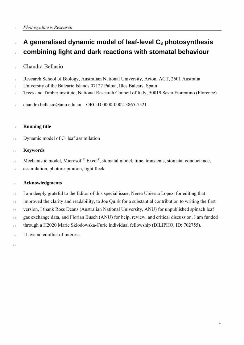
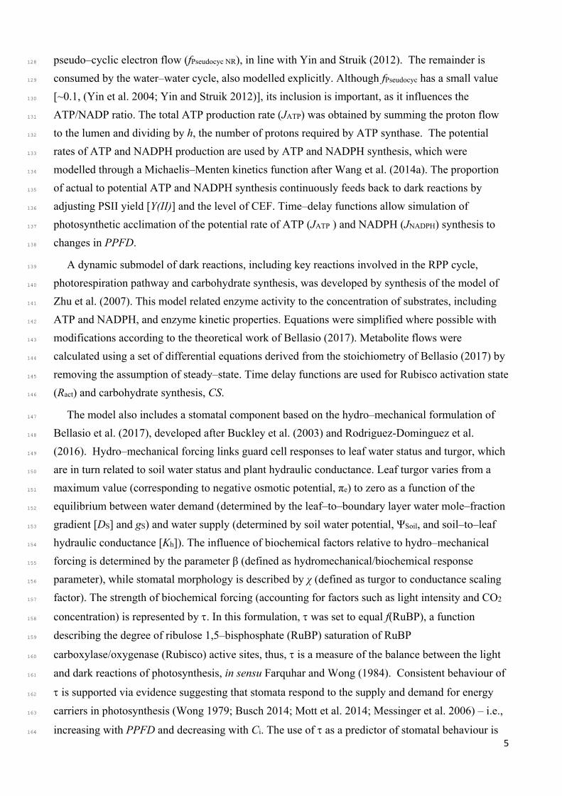
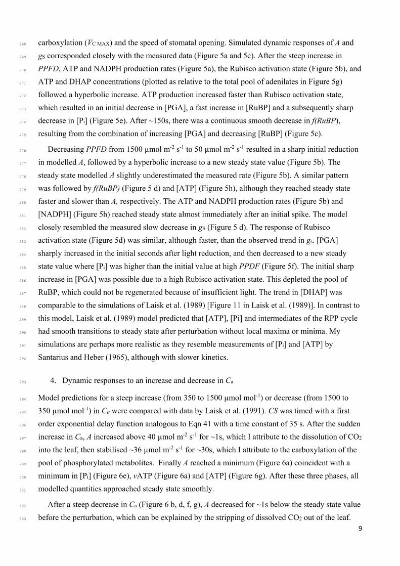
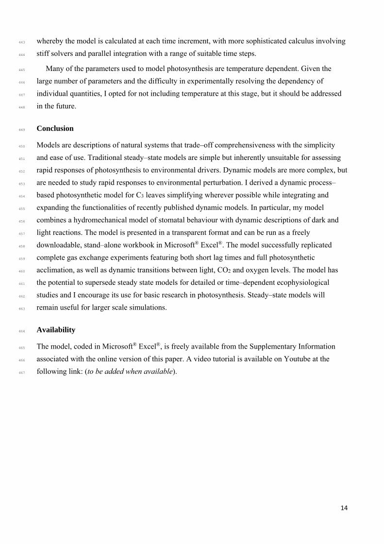
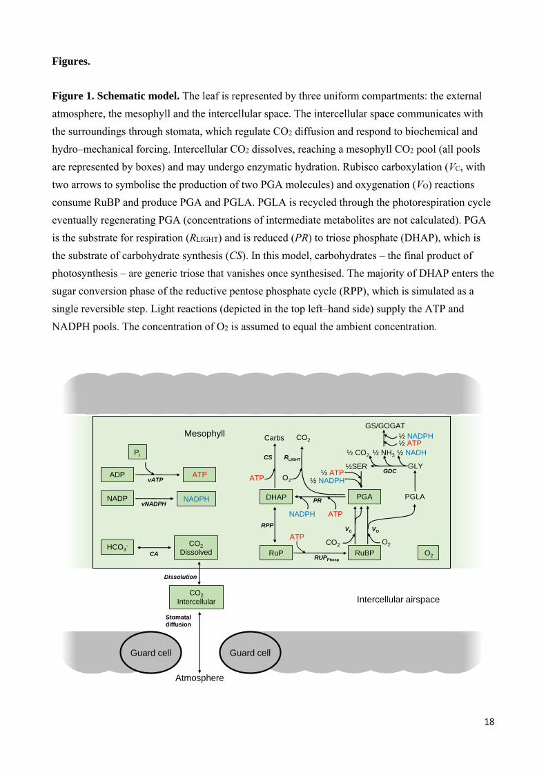
Figure 1. Schematic model. The leaf is represented by three uniform compartments: the external

atmosphere, the mesophyll and the intercellular space. The intercellular space communicates with

the surroundings through stomata, which regulate CO2 diffusion and respond to biochemical and

hydro–mechanical forcing. Intercellular CO2 dissolves, reaching a mesophyll CO2 pool (all pools

are represented by boxes) and may undergo enzymatic hydration. Rubisco carboxylation (VC, with

two arrows to symbolise the production of two PGA molecules) and oxygenation (VO) reactions

consume RuBP and produce PGA and PGLA. PGLA is recycled through the photorespiration cycle

eventually regenerating PGA (concentrations of intermediate metabolites are not calculated). PGA

is the substrate for respiration (RLIGHT) and is reduced (PR) to triose phosphate (DHAP), which is

the substrate of carbohydrate synthesis (CS). In this model, carbohydrates – the final product of

photosynthesis – are generic triose that vanishes once synthesised. The majority of DHAP enters the

sugar conversion phase of the reductive pentose phosphate cycle (RPP), which is simulated as a

single reversible step. Light reactions (depicted in the top left–hand side) supply the ATP and

NADPH pools. The concentration of O2 is assumed to equal the ambient concentration.

Guard cell Guard cell

Carbs

DHAP PGA

RuP RuBP

ATP

PGLA

VC

RUPPhosp

RPP

CO2

O2

RLIGHT

CO2

CS

O2

VO

½ CO2 ½ NADH

½ ATP

PR

ATPNADPH

GLY½SER

½ NH3

½ NADPHGDC

ATP

½ ATP

Atmosphere

Stomataldiffusion

CO2Intercellular

CO2

DissolvedHCO3

-

CA

Dissolution

ADP

Pi

ATPvATP

NADP NADPHvNADPH

O2

½ NADPHGS/GOGAT

Intercellular airspace

Mesophyll

 

19  

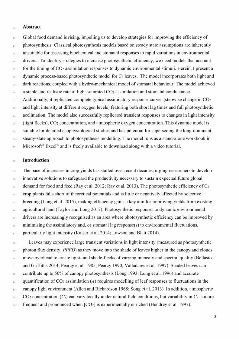
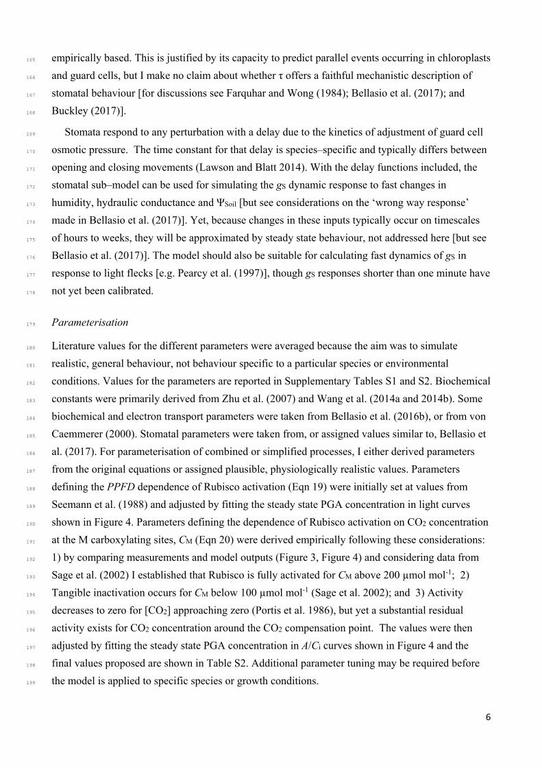
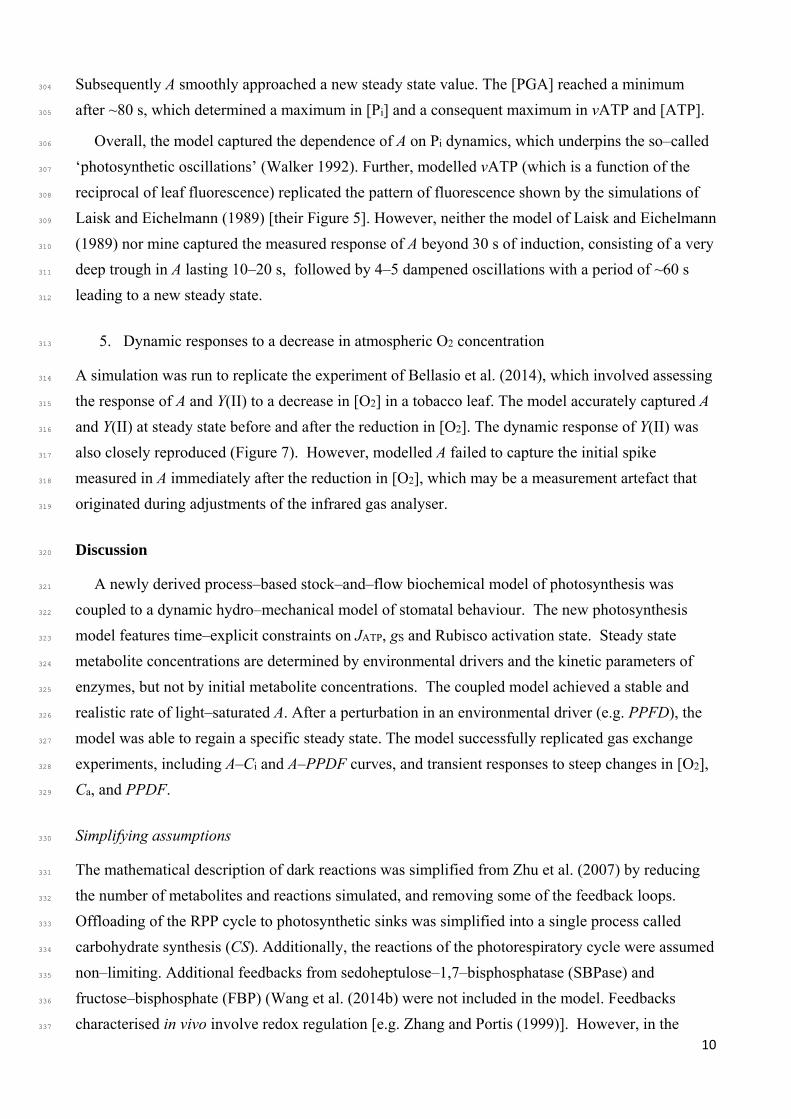
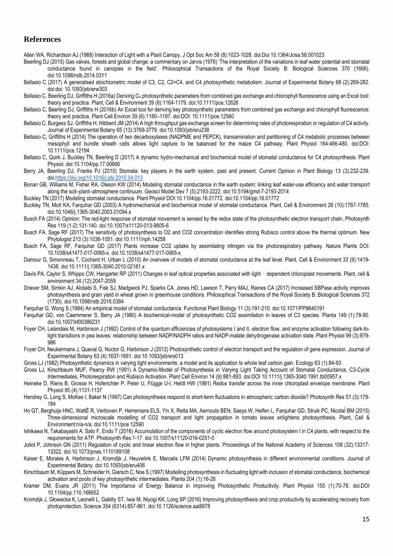
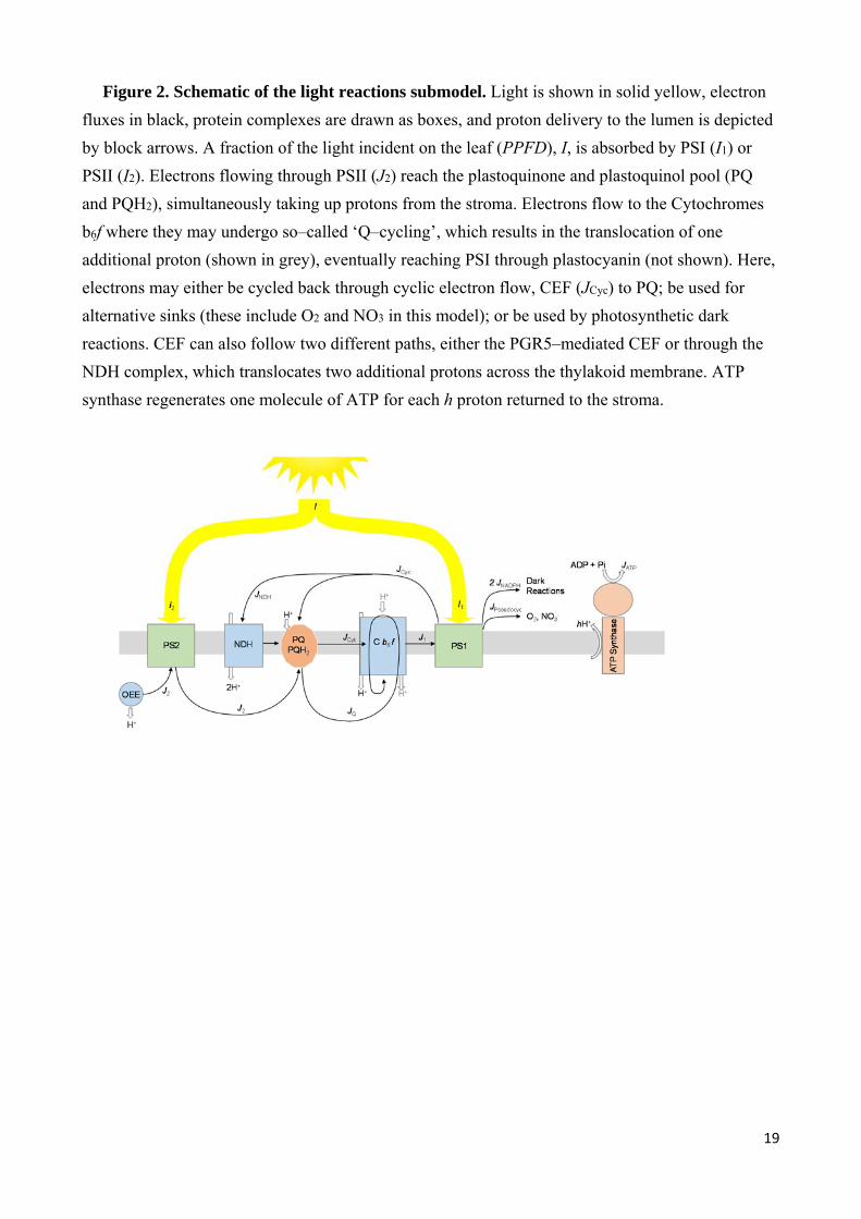
Figure 2. Schematic of the light reactions submodel. Light is shown in solid yellow, electron

fluxes in black, protein complexes are drawn as boxes, and proton delivery to the lumen is depicted

by block arrows. A fraction of the light incident on the leaf (PPFD), I, is absorbed by PSI (I1) or

PSII (I2). Electrons flowing through PSII (J2) reach the plastoquinone and plastoquinol pool (PQ

and PQH2), simultaneously taking up protons from the stroma. Electrons flow to the Cytochromes

b6f where they may undergo so–called ‘Q–cycling’, which results in the translocation of one

additional proton (shown in grey), eventually reaching PSI through plastocyanin (not shown). Here,

electrons may either be cycled back through cyclic electron flow, CEF (JCyc) to PQ; be used for

alternative sinks (these include O2 and NO3 in this model); or be used by photosynthetic dark

reactions. CEF can also follow two different paths, either the PGR5–mediated CEF or through the

NDH complex, which translocates two additional protons across the thylakoid membrane. ATP

synthase regenerates one molecule of ATP for each h proton returned to the stroma.

 

20  

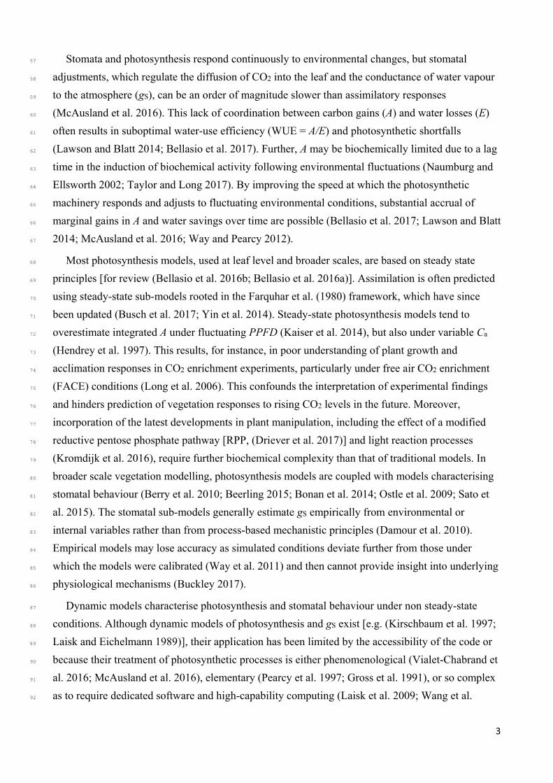
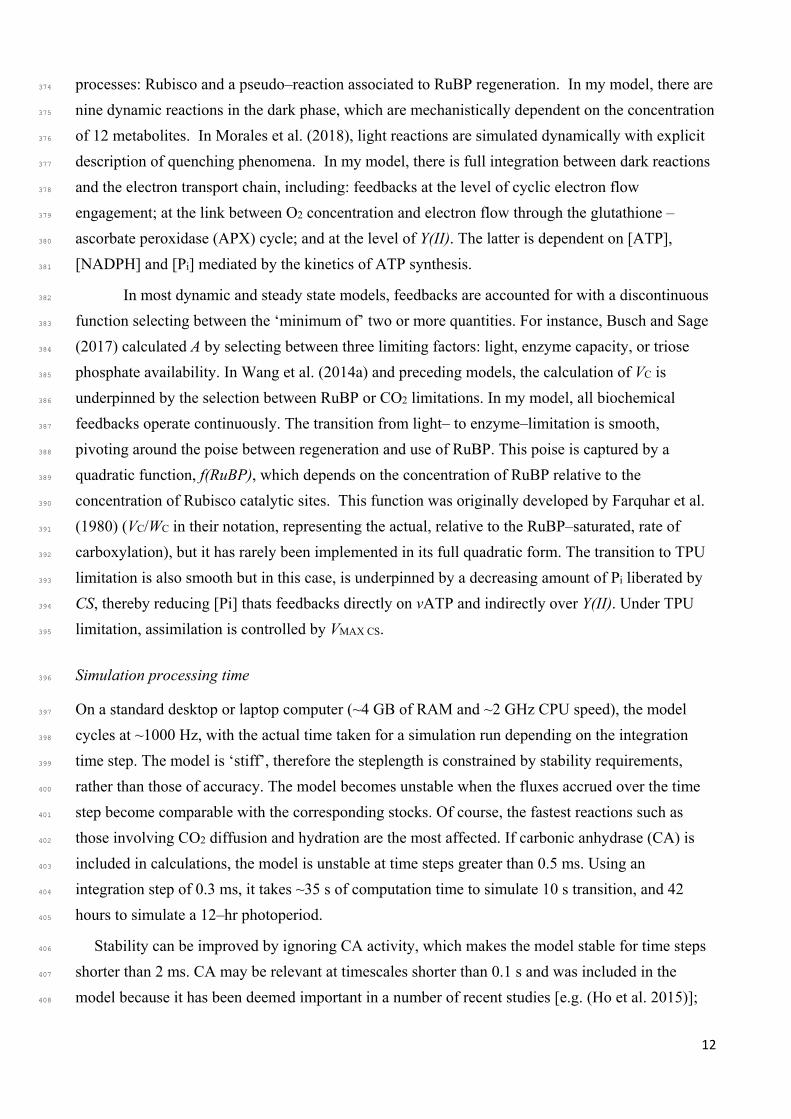
Figure 3. Simulated A–Ci and A–PPFD response curves. Gas exchange experiments simulated

with time increments of 1.5 ms. Modelled responses of assimilation rate, A (a–b), stomatal

conductance, gS (c–d), and NADPH production rate, vNADPH (e–f) to incident irradiance, PPFD

(left) and [CO2] in the intercellular space, Ci (right) at 21% O2 (open circles) and at 2% O2 (open

triangles). The model is plotted against data from Bellasio et al. (2016b) measured under 21% O2

(closed circles) and at 2% O2 (filled triangles). Error bars show ±1 SE. Details of parameterisation

are given in supporting Tables S1 and S2.

 

PPFD / mol m-2s-1100 300 500 700 900 1100 1300 1500

VN

AD

PH /

m

ol m

-2 s

-1

20

40

60

80

100

A /

m

ol m

-2 s

-1

5

15

25

35

Modelled Ambient O2

Measured Ambient O2

Modelled Low O2

Measured Low O2

g S /

mo

l m-2 s

-1

0.05

0.15

0.25

0.35

0.45

Ci / mol mol-1100 300 500 700 900 1100

VN

AD

PH /

m

ol m

-2 s

-1

20

40

60

80

100

g S /

mo

l m-2 s

-1

0.05

0.15

0.25

0.35

0.45

A /

m

ol m

-2 s

-1

5

15

25

35

a b

c d

e f

 

21  

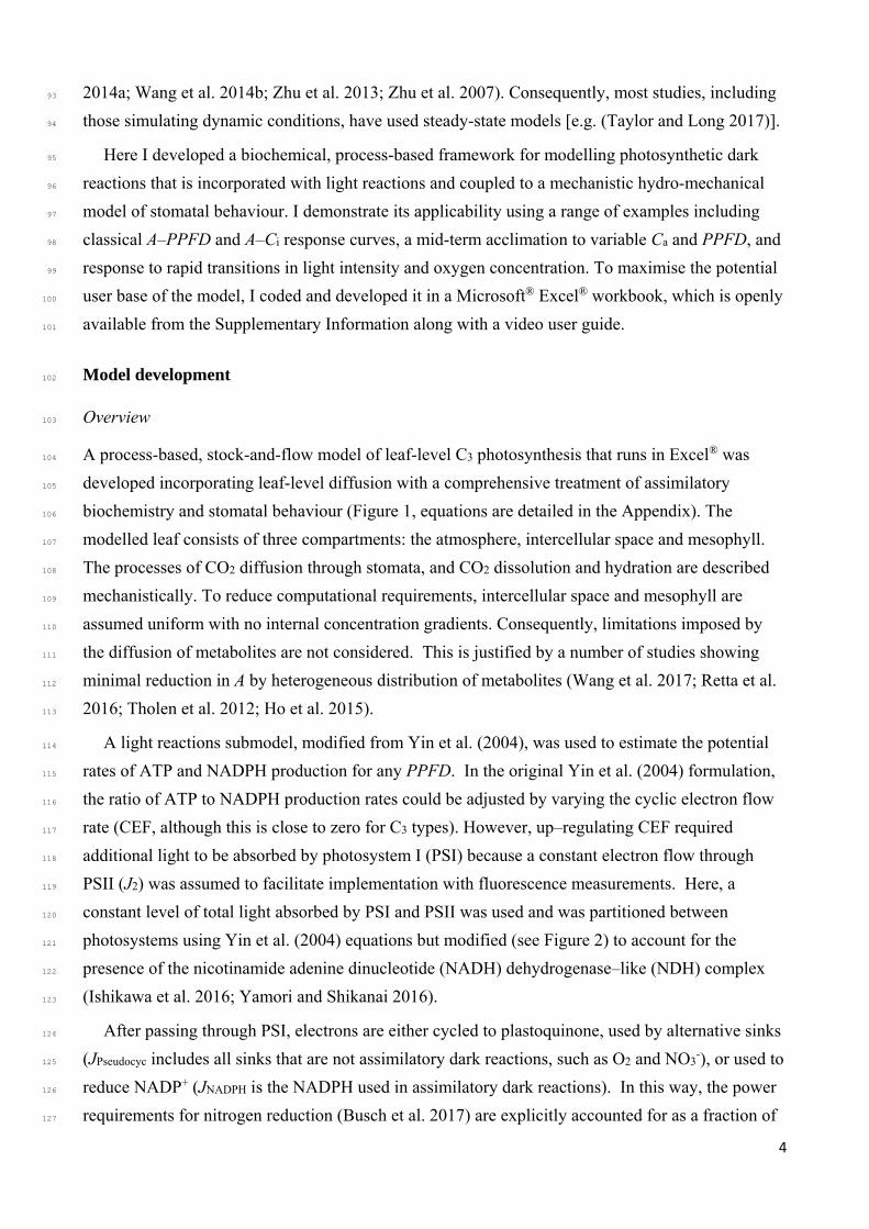
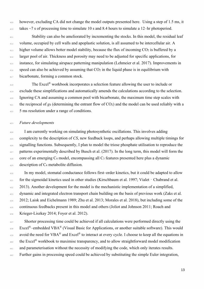
Figure 4. Metabolite concentrations at steady state. The model was run for 1800 s at different

levels of PPFD (left–hand panels) or Ca (right–hand panels) until quasi steady state was reached.

Panels (a–b): RuBP concentration; Panels (c–d): PGA concentration; Panels (d–e): relative Rubisco

activity calculated as f(RuBP) × Ract. The model (open symbols) is plotted against data from von

Caemmerer and Edmondson (1986) (closed symbols) measured under 21% O2 (circles) and at 2%

O2 (triangles). Parameterisation was maintained from previous simulation, see supporting Tables S1

and S2.

 

PPFD / mol m-2s-1100 300 500 700 900 1100 1300 1500

Rub

isco

Re

l. A

ctiv

ity

0.2

0.4

0.6

0.8

1.0

RuB

P /

m

ol m

-2

50

100

150

200Modelled Ambient O2

Measured Ambient O2

Modelled Low O2

PG

A

/ m

ol m

-2

100

200

300

Ci / mol mol-1100 300 500 700 900 1100

Rub

isco

Re

l. A

ctiv

ity

0.2

0.4

0.6

0.8

1.0

PG

A /

m

ol m

-2

100

200

300

RuB

P /

m

ol m

-2

50

100

150

200Measured Low O2

a b

c d

e f

 

22  

Figure 5. Response to a transition from low– to high–light and from high– to low–light. Circles

show the average of n=3 measurements taken on spinach (Spinacia oleracea, courtesy of Ross

Deans, unpublished). The leaf was acclimated under a PPFD of 50 µmol m-2 s-1 (left) or 1500 µmol

m-2 s-1 (right) until steady state was reached, then PPFD was increased to 1500 µmol m-2 s-1 or

decreased to 50 µmol m-2 s-1 and the variation in leaf level assimilation, A (a, b), stomatal

conductance, gS (c, d) and CO2 concentration in the intercellular space, were recorded every 10 s.

Lines show model outputs: rate of ATP and NADPH synthesis, and A (panels a and b); gS, f(RuBP)

and Rubisco activation state (c and d); concentrations of metabolites (e and f); ATP and NADPH

concentrations (g and h). For simulations, Ca was the same as in the measurement cuvette

(350 µmol mol-1), VC MAX = 0.18 mmol m-2 s-1, stomatal characteristics were adjusted at χβ = 0.8

mol air MPa-1, τ0=-0.12, Ki=3600 s; Kd=1200 s all other parameters were maintained from previous

simulations (supporting Tables S1 and S2).

PPFD / mol m-2s-10 200 400 600 800 1000 1200 1400

g S ,

R.

Act

, f

(Ru

BP

)

0.2

0.4

0.6

0.8

1.0

Modelled gS

Measured gS

f(RuBP) Rub. Act. St.

a

c

time / s0 200 400 600 800 1000 1200 1400

Co

nce

ntra

tion

/ m

M

2

4

6

8e

time / s0 200 400 600 800 1000 1200 1400

Rat

io

0.2

0.4

0.6

0.8

[ATP] / Atot[NADPH] / NTot

PPFD / mol m-2s-10 200 400 600 800 1000

Flu

x / m

ol m

-2 s

-1

2

4

6

8

PPFD / mol m-2s-10 200 400 600 800 1000

g S ,

R.

Act

, f

(Ru

BP

)

0.2

0.4

0.6

0.8

1.0

b

d

time / s

Co

nce

ntra

tion

/ m

M

2

4

6

8

PGADHAPPi RuBP

f

time / s0 200 400 600 800 1000

Rat

io

0.2

0.4

0.6

0.8[ATP] / Atot[NADPH] /NTot

g h

Flu

x / m

ol m

-2 s

-1

10

20

30

40

50

PGA

DHAP

Pi

RuBP

Modelled A

Measured A

vATP/3

vNADPH/2

Modelled gS

Measured gS

f(RuBP)

Rub. Act. St.

Modelled A

Measured A

vATP/3

vNADPH/2

 

23  

Figure 6. Modelled response to a transition from ambient– to high–CO2 and from high– to

ambient CO2. The model was run at a Ca of 350 µmol mol-1 (left) or of 1500 µmol mol-1 (right)

until steady state was reached. Then Ca was increased to 1500 µmol mol-1 or decreased to 350 µmol

mol-1. Lines show modelled rates of ATP and NADPH synthesis, and A (panels a and b); gS,

f(RuBP) and Rubisco activation state (c and d); concentrations of metabolites (e and f); ATP and

NADPH concentrations (g and h). Parameters were the same as in Figure 5.

PPFD / mol m-2s-10 50 100 150 200 250

gS ,

R.

Act

, f

(Ru

BP

)

0.2

0.4

0.6

0.8

1.0

Modelled gS

f(RuBP) Rub. Act. St.

a

c

time / s0 50 100 150 200 250

Co

nce

ntr

atio

n /

mM

2

4

6

8

e

time / s0 50 100 150 200 250

Ra

tio

0.2

0.4

0.6

0.8

[ATP] / Atot[NADPH] / NTot

Flu

x / m

ol m

-2 s

-1

10

20

30

40

50

gS ,

R.

Act

, f

(Ru

BP

)

0.2

0.4

0.6

0.8

1.0

b

dC

on

cen

trat

ion

/ m

M

2

4

6

8 PGADHAPPi RuBP

f

time / s0 50 100 150 200

Ra

tio

0.2

0.4

0.6

0.8

[ATP] / Atot[NADPH] /NTot

g h

Flu

x / m

ol m

-2 s

-1

10

20

30

40

50

PGA DHAP

Pi

RuBP

Modelled AvATP/3

vNADPH/2

Modelled gS

f(RuBP)

Rub. Act. St.

Modelled A

vATP/3

vNADPH/2

 

24  

Figure 7. Response to a transition from ambient to low atmospheric oxygen concentration.

Open symbols show tobacco measurements from Bellasio et al. (2014) where the leaf was

acclimated under a PPFD = 300 µmol m-2 s-1 and Ca = 200 µmol mol-1 until steady state was

reached. Then the background gas was switched to 2% O2 and the variation in leaf level

assimilation (A, triangles), and yield of photosystem II (Y(II), squares) were recorded every ~17 s.

The model replicated this experiment. The solid line shows modelled leaf level assimilation, while

dots show modelled Y(II) calculated as . ∙ ∙

, where s is an energy conversion

coefficient. In the model, Ca was set to equal Ca in the measurement cuvette, while all other

parameters were maintained from Figure 3 and 4 (supporting Tables S1 and S2).

Time / s100 200 300 400 500 600

Net

Ass

imila

tion

/

mo

l m-2 s

-1

6.0

9.0

12.0

15.0

18.0Y

(II)

0.1

0.3

0.5

0.7

AY(II)Modelled A

Modelled Y(II)

2% O2Ambient O2

 

25  

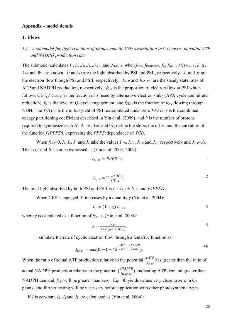
Appendix – model details

1. Flows

1.1. A submodel for light reactions of photosynthetic CO2 assimilation in C3 leaves: potential ATP

and NADPH production rate

The submodel calculates I1, I2, J1, J2, JATP, and JNADPH when fCyc, fPseudocyc, fQ, fNDH, Y(II)LL, s, h, αV,

V0V and θV are known. I1 and I2 are the light absorbed by PSI and PSII, respectively. J1 and J2 are

the electron flow though PSI and PSII, respectively. JATP and JNADPH are the steady state rates of

ATP and NADPH production, respectively. fCyc is the proportion of electron flow at PSI which

follows CEF, fPseudocyc is the fraction of J1 used by alternative electron sinks (APX cycle and nitrate

reduction), fQ is the level of Q–cycle engagement, and fNDH is the fraction of fCyc flowing through

NDH. The Y(II) LL is the initial yield of PSII extrapolated under zero PPFD, s is the combined

energy partitioning coefficient described in Yin et al. (2009), and h is the number of protons

required to synthesize each ATP. αV, V0V and θV, define the slope, the offset and the curvature of

the function f′(PPFD), expressing the PPFD dependence of Y(II).

When fCyc=0, I1, I2, J1 and J2 take the values I1, 0, I2, 0, J1, 0 and J2, 0 respectively and J1, 0=J2,0.

Then I2, 0 and I1, 0 can be expressed as (Yin et al. 2004, 2009):

, ∙ , 1

,, , 2

The total light absorbed by both PSI and PSII is I = I1, 0 + I2, 0, and I<PPFD.

When CEF is engaged, I1 increases by a quantity χ (Yin et al. 2004):

1 , , 3

where χ is calculated as a function of fCyc as (Yin et al. 2004):

. 4

I simulate the rate of cyclic electron flow through a tentative function as:

max 0, 1 15 ATP NADPH . 4b

When the ratio of actual ATP production relative to the potential (

is greater than the ratio of

actual NADPH production relative to the potential , indicating ATP demand greater than

NADPH demand, fCyc will be greater than zero. Eqn 4b yields values very close to zero in C3

plants, and further testing will be necessary before application with other photosynthetic types.

If I is constant, I2, J2 and J1 are calculated as (Yin et al. 2004):

 

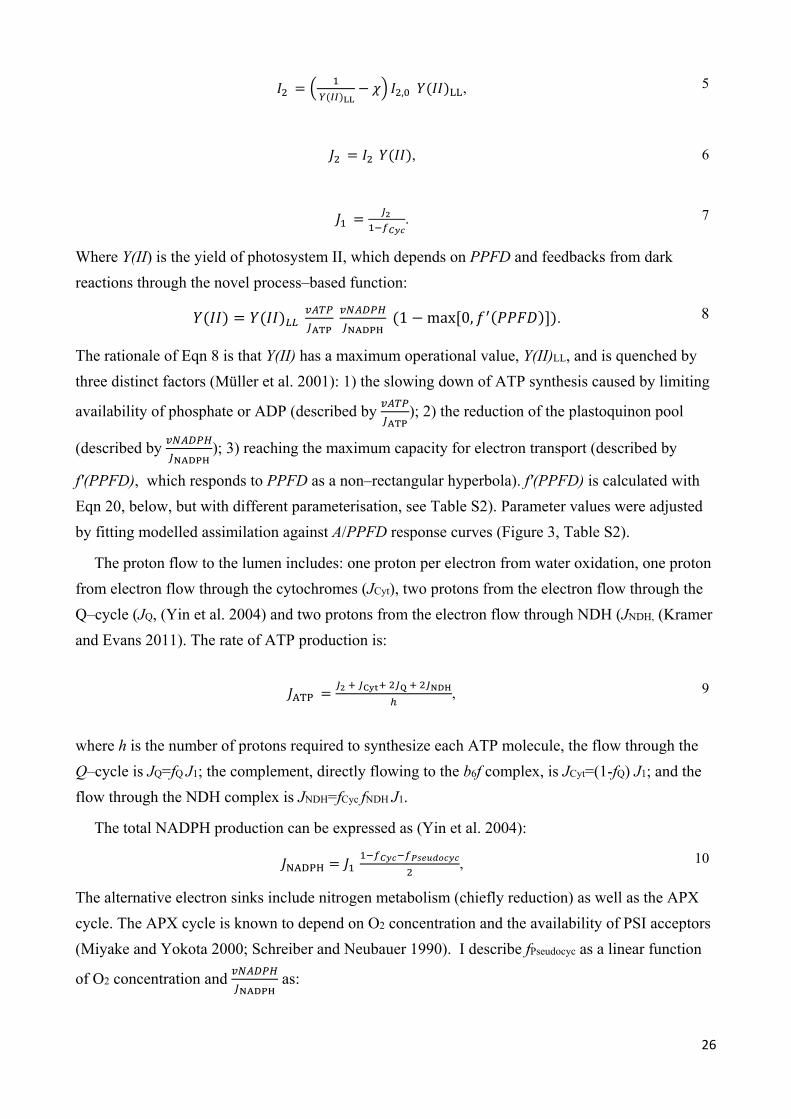
26  

, , 5

, 6

. 7

Where Y(II) is the yield of photosystem II, which depends on PPFD and feedbacks from dark

reactions through the novel process–based function:

1 max 0, . 8

The rationale of Eqn 8 is that Y(II) has a maximum operational value, Y(II)LL, and is quenched by

three distinct factors (Müller et al. 2001): 1) the slowing down of ATP synthesis caused by limiting

availability of phosphate or ADP (described by ); 2) the reduction of the plastoquinon pool

(described by ); 3) reaching the maximum capacity for electron transport (described by

f′(PPFD), which responds to PPFD as a non–rectangular hyperbola). f′(PPFD) is calculated with

Eqn 20, below, but with different parameterisation, see Table S2). Parameter values were adjusted

by fitting modelled assimilation against A/PPFD response curves (Figure 3, Table S2).

The proton flow to the lumen includes: one proton per electron from water oxidation, one proton

from electron flow through the cytochromes (JCyt), two protons from the electron flow through the

Q–cycle (JQ, (Yin et al. 2004) and two protons from the electron flow through NDH (JNDH, (Kramer

and Evans 2011). The rate of ATP production is:

, 9

where h is the number of protons required to synthesize each ATP molecule, the flow through the

Q–cycle is JQ=fQ J1; the complement, directly flowing to the b6f complex, is JCyt=(1-fQ) J1; and the

flow through the NDH complex is JNDH=fCyc fNDH J1.

The total NADPH production can be expressed as (Yin et al. 2004):

, 10

The alternative electron sinks include nitrogen metabolism (chiefly reduction) as well as the APX

cycle. The APX cycle is known to depend on O2 concentration and the availability of PSI acceptors

(Miyake and Yokota 2000; Schreiber and Neubauer 1990). I describe fPseudocyc as a linear function

of O2 concentration and as:

 

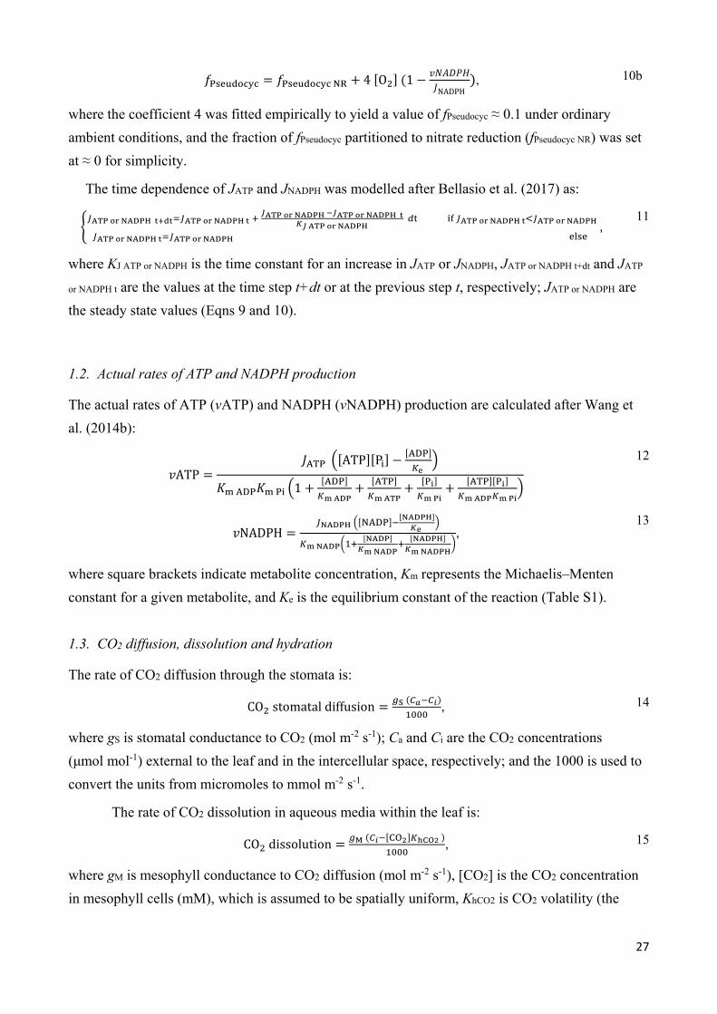
27  

4 O 1NADPH

, 10b

where the coefficient 4 was fitted empirically to yield a value of fPseudocyc ≈ 0.1 under ordinary

ambient conditions, and the fraction of fPseudocyc partitioned to nitrate reduction (fPseudocyc NR) was set

at ≈ 0 for simplicity.

The time dependence of JATP and JNADPH was modelled after Bellasio et al. (2017) as:

,

11

where KJ ATP or NADPH is the time constant for an increase in JATP or JNADPH, JATP or NADPH t+dt and JATP

or NADPH t are the values at the time step t+dt or at the previous step t, respectively; JATP or NADPH are

the steady state values (Eqns 9 and 10).

1.2. Actual rates of ATP and NADPH production

The actual rates of ATP (vATP) and NADPH (vNADPH) production are calculated after Wang et

al. (2014b):

ATPATP P

1

12

NADPH , 13

where square brackets indicate metabolite concentration, Km represents the Michaelis–Menten

constant for a given metabolite, and Ke is the equilibrium constant of the reaction (Table S1).

1.3. CO2 diffusion, dissolution and hydration

The rate of CO2 diffusion through the stomata is:

CO stomatal diffusion , 14

where gS is stomatal conductance to CO2 (mol m-2 s-1); Ca and Ci are the CO2 concentrations

(μmol mol-1) external to the leaf and in the intercellular space, respectively; and the 1000 is used to

convert the units from micromoles to mmol m-2 s-1.

The rate of CO2 dissolution in aqueous media within the leaf is:

CO dissolution , 15

where gM is mesophyll conductance to CO2 diffusion (mol m-2 s-1), [CO2] is the CO2 concentration

in mesophyll cells (mM), which is assumed to be spatially uniform, KhCO2 is CO2 volatility (the

 

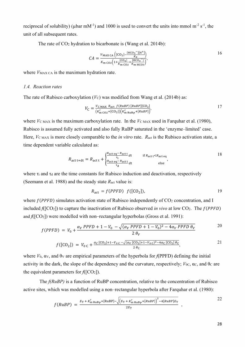
28  

reciprocal of solubility) (µbar mM-1) and 1000 is used to convert the units into mmol m-2 s-1, the

unit of all subsequent rates.

The rate of CO2 hydration to bicarbonate is (Wang et al. 2014b):

, 16

where VMAX CA is the maximum hydration rate.

1.4. Reaction rates

The rate of Rubisco carboxylation (VC) was modified from Wang et al. (2014b) as:

, 17

where VC MAX is the maximum carboxylation rate. In the VC MAX used in Farquhar et al. (1980),

Rubisco is assumed fully activated and also fully RuBP saturated in the ‘enzyme–limited’ case.

Here, VC MAX is more closely comparable to the in vitro rate. Ract is the Rubisco activation state, a

time dependent variable calculated as:

,

18

where τi and τd are the time constants for Rubisco induction and deactivation, respectively

(Seemann et al. 1988) and the steady state Ract value is:

CO , 19

where simulates activation state of Rubisco independently of CO2 concentration, and I

included f([CO2]) to capture the inactivation of Rubisco observed in vivo at low CO2. The

and f([CO2]) were modelled with non–rectangular hyperbolas (Gross et al. 1991):

1 1 4

2

20

CO

, 21

where V0, αV, and θV are empirical parameters of the hyperbola for f(PPFD) defining the initial

activity in the dark, the slope of the dependency and the curvature, respectively; V0C, αC, and θC are

the equivalent parameters for f([CO2]).

The f(RuBP) is a function of RuBP concentration, relative to the concentration of Rubisco

active sites, which was modelled using a non–rectangular hyperbola after Farquhar et al. (1980):

, 22

 

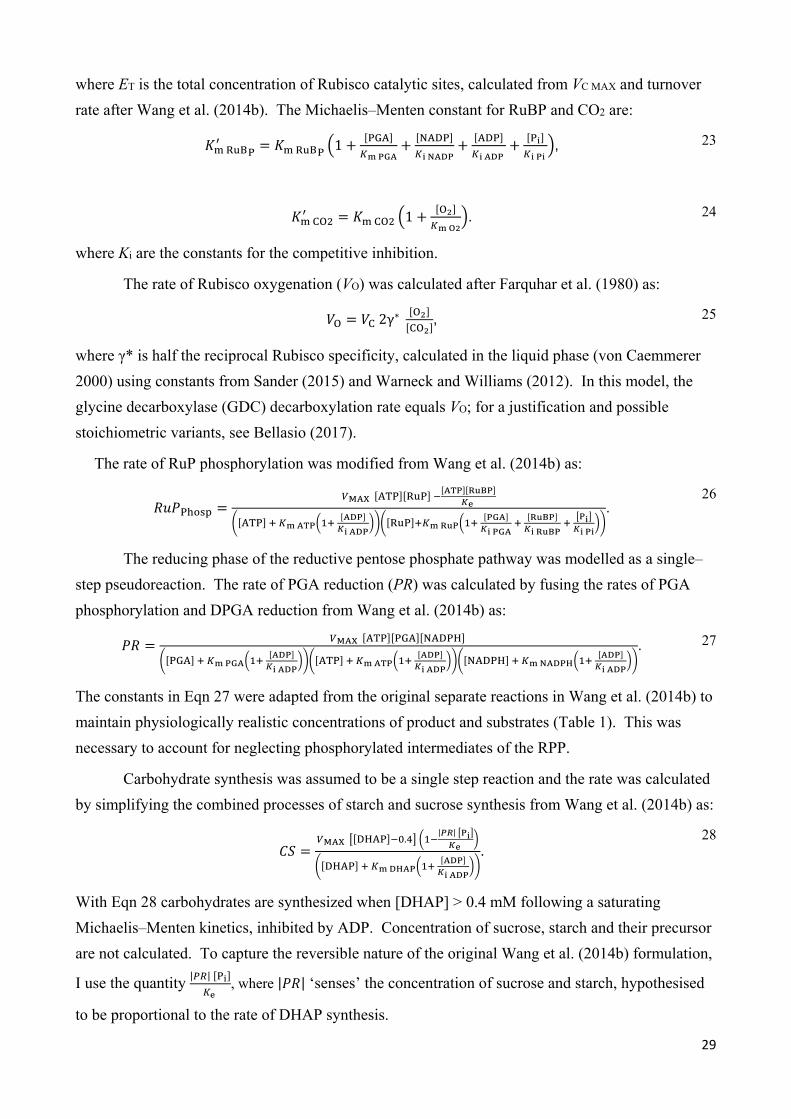
29  

where ET is the total concentration of Rubisco catalytic sites, calculated from VC MAX and turnover

rate after Wang et al. (2014b). The Michaelis–Menten constant for RuBP and CO2 are:

1 , 23

1 . 24

where Ki are the constants for the competitive inhibition.

The rate of Rubisco oxygenation (VO) was calculated after Farquhar et al. (1980) as:

2γ∗ , 25

where γ* is half the reciprocal Rubisco specificity, calculated in the liquid phase (von Caemmerer

2000) using constants from Sander (2015) and Warneck and Williams (2012). In this model, the

glycine decarboxylase (GDC) decarboxylation rate equals VO; for a justification and possible

stoichiometric variants, see Bellasio (2017).

The rate of RuP phosphorylation was modified from Wang et al. (2014b) as:

. 26

The reducing phase of the reductive pentose phosphate pathway was modelled as a single–

step pseudoreaction. The rate of PGA reduction (PR) was calculated by fusing the rates of PGA

phosphorylation and DPGA reduction from Wang et al. (2014b) as:

. 27

The constants in Eqn 27 were adapted from the original separate reactions in Wang et al. (2014b) to

maintain physiologically realistic concentrations of product and substrates (Table 1). This was

necessary to account for neglecting phosphorylated intermediates of the RPP.

Carbohydrate synthesis was assumed to be a single step reaction and the rate was calculated

by simplifying the combined processes of starch and sucrose synthesis from Wang et al. (2014b) as:

.| |

. 28

With Eqn 28 carbohydrates are synthesized when [DHAP] > 0.4 mM following a saturating

Michaelis–Menten kinetics, inhibited by ADP. Concentration of sucrose, starch and their precursor

are not calculated. To capture the reversible nature of the original Wang et al. (2014b) formulation,

I use the quantity | |

, where | | ‘senses’ the concentration of sucrose and starch, hypothesised

to be proportional to the rate of DHAP synthesis.

 

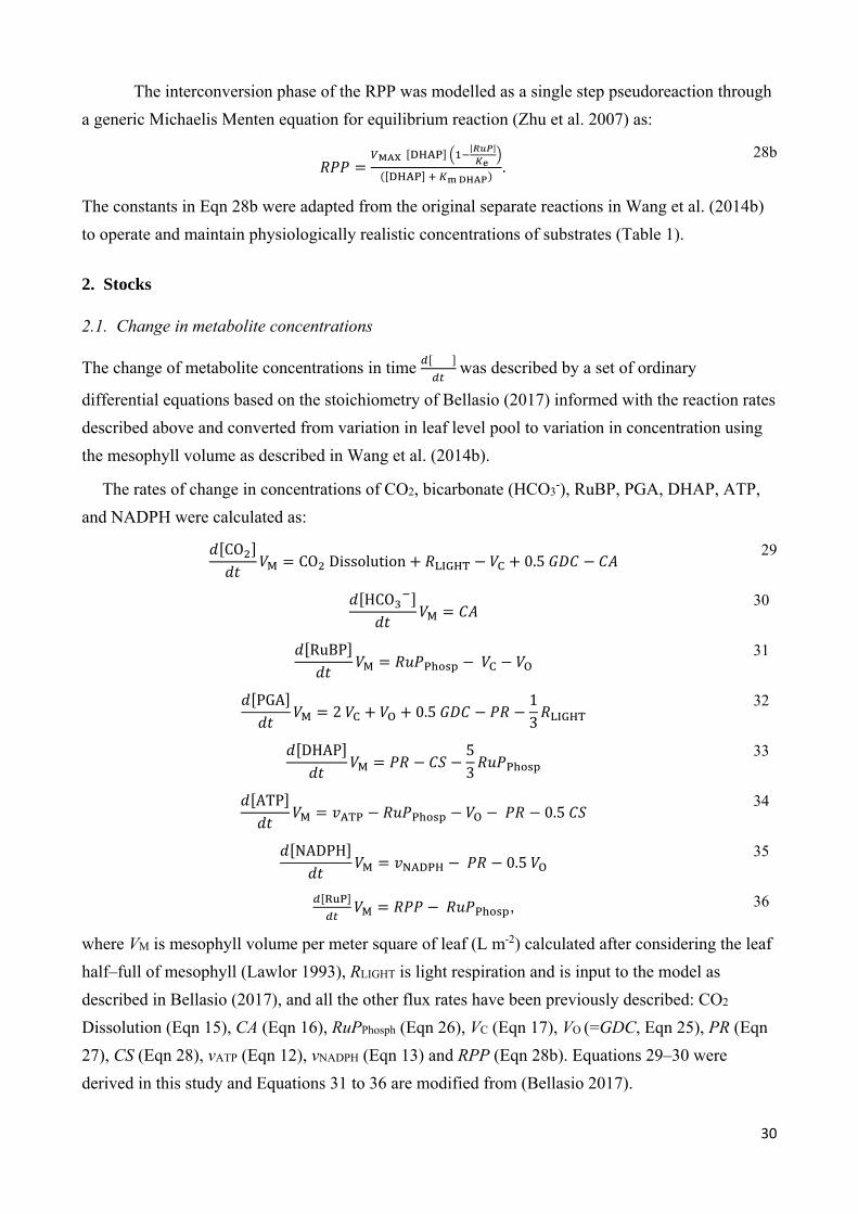
30  

The interconversion phase of the RPP was modelled as a single step pseudoreaction through

a generic Michaelis Menten equation for equilibrium reaction (Zhu et al. 2007) as:

| |

. 28b

The constants in Eqn 28b were adapted from the original separate reactions in Wang et al. (2014b)

to operate and maintain physiologically realistic concentrations of substrates (Table 1).

2. Stocks

2.1. Change in metabolite concentrations

The change of metabolite concentrations in time was described by a set of ordinary

differential equations based on the stoichiometry of Bellasio (2017) informed with the reaction rates

described above and converted from variation in leaf level pool to variation in concentration using

the mesophyll volume as described in Wang et al. (2014b).

The rates of change in concentrations of CO2, bicarbonate (HCO3-), RuBP, PGA, DHAP, ATP,

and NADPH were calculated as:

COCO Dissolution 0.5

29

HCO

30

RuBP

31

PGA2 0.5

13

32

DHAP 53

33

ATP0.5

34

NADPH0.5

35

, 36

where VM is mesophyll volume per meter square of leaf (L m-2) calculated after considering the leaf

half–full of mesophyll (Lawlor 1993), RLIGHT is light respiration and is input to the model as

described in Bellasio (2017), and all the other flux rates have been previously described: CO2

Dissolution (Eqn 15), CA (Eqn 16), RuPPhosph (Eqn 26), VC (Eqn 17), VO (=GDC, Eqn 25), PR (Eqn

27), CS (Eqn 28), vATP (Eqn 12), vNADPH (Eqn 13) and RPP (Eqn 28b). Equations 29–30 were

derived in this study and Equations 31 to 36 are modified from (Bellasio 2017).

 

31  

2.2. Concentrations determined from total metabolite pools

The concentrations of ADP, NADP+, and phosphate ( P ) are calculated simply by subtraction from

a total pool:

ADP ATP 37

NADP NADPH 38

P PGA DHAP RuP 2 RuBP ATP , 39

where ATot, NTot, and PiTot are the total pools of adenylates, nicotinamides and phosphate,

respectively.

3. The hydro–mechanical model of stomatal behaviour

The model calculates gS after Bellasio et al. (2017) as:

max , Soil

h S, 40

where χβ is a combined parameter scaling turgor–to–conductance and the hydromechanical–to–

biochemical response; τ is the sensor of biochemical forcing;ΨSoil is soil water potential; e is

epidermal osmotic pressure; Rh is the effective hydraulic resistance to the epidermis, calculated as

1/Kh, the corresponding hydraulic conductance; and DS is the leaf–to–boundary layer H2O mole

fraction gradient, a measure of vapour pressure deficit, VPD. The parameter τ encompasses the

biochemical components of the model and is calculated from f(RuBP) as:

τ , 41

where τ0, the basal level of τ, was manually assigned. Stomatal dynamics were accounted for by

describing the time dependence of gS with a set of recursive equations (Bellasio et al. 2017):

,

42

where gSt+dt and gSt are the gS values at the time step t+dt or at the previous step t, respectively; gS is

the steady state value (Eqn 40), Ki and Kd are the time constants for an increase and decrease in gS,

respectively.