A general modeling framework for the operational …cepac.cheme.cmu.edu/pasilectures/pinto/revpaper-NP.pdf · Computers and Chemical Engineering 28 (2004) 871–896 A general modeling

Computers and Chemical Engineering 28 (2004) 871–896

A general modeling framework for the operationalplanning of petroleum supply chains

Sérgio M.S. Neiroa,1, José M. Pintoa,b,∗,2

a Department of Chemical Engineering, University of São Paulo, 05508-900 São Paulo, SP, Brazilb Department of Chemical Engineering and Chemistry, Polytechnic University, Brooklyn, NY 11201, USA

Abstract

In the literature, optimization models deal with planning and scheduling of several subsystems of the petroleum supply chain such asoilfield infrastructure, crude oil supply, refinery operations and product transportation. The focus of the present work is to propose a generalframework for modeling petroleum supply chains. As a starting point, processing units are modeled based on the framework developed byPinto et al. [Computers and Chemical Engineering 24 (2000) 2259]. Particular frameworks are then proposed to storage tanks and pipelines.Nodes of the chain are considered as grouped elementary entities that are interconnected by intermediate streams. The complex topologyis then built by connecting the nodes representing refineries, terminals and pipeline networks. Decision variables include stream flow rates,properties, operational variables, inventory and facilities assignment. The resulting multiperiod model is a large-scale MINLP. The proposedmodel is applied to a real-world corporation and results show model performance by analyzing different scenarios.© 2003 Elsevier Ltd. All rights reserved.

Keywords: Petroleum complex; Supply chain management; Mixed-integer optimization

1. Introduction

Companies have been forced to overstep their physicalfrontiers and to visualize the surrounding business environ-ment before planning their activities. Range vision shouldcover all members that participate direct or indirectly in thework to satisfy a customer necessity. Coordination of thisvirtual corporation may result in benefits for all members ofthe chain individually.Beamon (1998)defines such virtualcorporation as an integrated process wherein a number ofbusiness entities (suppliers, manufacturers, distributors andretailers) work together in an effort to acquire raw materi-als, convert them into specified final products and deliverthese final products to retailers. Under another point of view,Tan (2001)states that there is a definition of supply chainmanagement (SCM), which emerges from transportation andlogistics literature of the wholesaling and retailing indus-try that emphasizes the importance of physical distributionand integrated logistics. According toLamming (1996), this

∗ Corresponding author. Tel.:+1-718-260-3569;fax: +1-718-260-3125.

E-mail address: [email protected] (J.M. Pinto).1 Tel.: +55-11-3091-2237; fax:+55-11-3813-2380.2 Tel.: +1-718-260-3569; fax:+1-718-260-3125.

is probably where the term supply chain management wasoriginally used.

According toThomas and Griffin (1996), current researchin the area of SCM can be classified in three categories:Buyer–Vendor, production–distribution and inventory–dis-tribution coordination. The authors present an extensive lit-erature review for each category.Vidal and Goetschalckx(1997) present a review of mixed integer problems (MIP)that focuses on the identification of the relevant factors in-cluded in formulations of the chain or its subsystems andalso highlights solution methodologies.

Bok, Grossmann, and Park (2000)present an appli-cation to the optimization of continuous flexible processnetworks. Modeling considers intermittent deliveries, pro-duction shortfalls, delivery delays, inventory profiles andjob changeovers. A bi-level solution methodology is pro-posed to reduce computational expense.Zhuo, Cheng, andHua (2000)introduce a supply chain model that involvesconflicting decisions in the objective function. Goal pro-gramming is used to solve the multi-objective optimizationproblem.Perea, Grossmann, Ydstie, and Tahmassebi (2000)andPerea-López, Grossmann, and Ydstie (2001)present anapproach that is capable of capturing the dynamic behaviorof the supply chain by modeling flow of materials and infor-mation within the supply chain. Information is considered

0098-1354/$ – see front matter © 2003 Elsevier Ltd. All rights reserved.doi:10.1016/j.compchemeng.2003.09.018

872 S.M.S. Neiro, J.M. Pinto / Computers and Chemical Engineering 28 (2004) 871–896

Nomenclature

Indices:p propertys streamt time periodu, u′ unitv operating variable

Sets:PIu properties of the inlet stream of unituPOu,s properties of outlet streams of unit uSOu outlet streams of unituT time periods{t|t = 1, . . . , NT}Uco product tanks at refinery sites dedicated to

supply local marketUdem product tanks that present direct demand

from a consumerUf petroleum tanksUIu units whose outlet streams feed unituUnc product tanks at refinery sites that

supply local and other marketsUOu,s units that are fed by streams of unit uUp product tanksUpipe units that represent pipelinesUport petroleum tanks that store the crude

oil from suppliersUpu processing units at refinery sitesUr product tanks at refineriesUSu ordered pairs unit/stream (u′, s) that

feeds unituUtank all storage tanks of the supply chainVOu operating variables of unitu

Parameters:Cinvu,t inventory cost of tanku at time periodtCpetu,t price of petroleumu (u ∈ Uport) at

time periodtCpu,t sale price of productu (u ∈ Up)

at time periodtCru fixed operating cost coefficient of unituCtu transportation cost for pipelineuCvu,v variable coefficient cost of

the operating variablev of unit uDemu,t demand of productu at time period

t (u ∈ Up)PFL

u,p,t lower bound of inlet propertyp of unit uat time periodt

PFUu,p,t upper bound of inlet propertyp of unit u

at time periodtPropu,s,p standard property valuep of the

outlet streams from unit uQFL

u lower bound for feed flow rate of unituQFU

u upper bound for feed flow rateof unit u

QGainu,s,v flow rate gain of outlet streams of unitu due to operating variableu

QSLu lower bound for outlet flow rate of unitu

QSUu upper bound for outlet flow rate of unitu

V Lu,v lower bound for operating variablev of

unit uVU

u,v upper bound for operating variablev ofunit u

VariablesIu,s,p,t mixture indices of propertyp of

streams of unit u at time periodtPFu,p,t propertyp of the feed stream at unitu

at time periodtPSu,s,p,t propertyp of the outlet streams at

unit u at time periodtQFu,t feed flow rate of unitu at time periodtQSu,s,t outlet flow rate of streams at

unit u at time periodtQu ′,s,u,t flow rate of streams between

units u′ andu at time periodtVolu,t inventory level of tanku at

time periodtVu,v,t operating variablev of unit u at time

periodtyu,s,u ′,t binary variable which assumes 1 if

tanku is chosen to supplyu′ with s attime periodt; 0 otherwise

Processing unit:CDi atmospheric distillation columniDEPROP C3/C4 separation unitFCCi fluid catalytic cracking unitiHTi hydrotreatment unitiPDA propane-deasphalting unitSOLVi solvent distillation columniUCi bun unitiUFN naphtha fraction unitUMTBE unit for MTBE productionURA aromatic reform unitURC catalytic reform unitUVGA alcoholization unitVDi vacuum distillation columni

Product tank:PBEN pool of benzenePC3 pool of C3PC4 pool of C4PDIL pool of kerosene for dilutionPDILT pool of dye diluentPDIN pool of regular dieselPDMA pool of maritime dieselPDME pool of metropolitan dieselPDO pool of decanted oil

S.M.S. Neiro, J.M. Pinto / Computers and Chemical Engineering 28 (2004) 871–896 873

PEXFO pool of fuel oil (exportation type)PFO1A pool of fuel oil (type 1A)PFO1B pool of fuel oil (type 1B)PFO4A pool of fuel oil (type 4A)PGC pool of fuel gasPGLA pool of jet gasolinePGLE pool of exportation gasolinePGLN pool of gasolinePGLP pool of LPGPJFUEL pool of jet fuelPLCO pool of light fuel oilPMTBE pool of MTBEPMTU pool of mineral terpentinePNAL pool of light naphthaPNAP pool of naphthaPNAT pool of treated naphthaPOC pool of fuel oilPOCBV pool of BV fuel oilPOCP pool of premium fuel oilPPGC pool of petroleum green bunPPQN pool of petrochemical naphthaPRAT pool of ATRPSOLB pool of rubber solventPTOL pool of toluenePXIL pool of xylene

Stream:ASFR asphalt residueATR atmospheric residueBEN benzeneC3 propaneC3C4 C3/C4 mixtureC4 butaneCN bun naphthaCRAN cracked naphthaDAO deasphalted oilDILT dye diluentDIN regular dieselDMA maritime dieselDME metropolitan dieselDO decanted oil from FCCFDSOL1 bottom solvent from SOLV1FDSOL2 bottom solvent from SOLV2GC fuel gasGLN gasolineHD heavy dieselHGO bun heavy gas oilHK hydrotreated keroseneHN heavy naphthaHNU heavy naphtha from UFNHTD hydrotreated dieselHTOL heavy tolueneJFUEL jet fuelK kerosene

LALC light alcoholLCO light fuel oilLD light dieselLGO bun light gas oilLN light naphthaLNU light naphtha from UFNMTBE methyl terc butyl etherOC fuel oilPGC petroleum green bunRAF rafinateRFOR reformRNU naphtha for reform from UFNSOLB rubber solventTOL tolueneTPSOL1 top solvent from SOLV1TPSOL2 top solvent from SOLV2VGO gas oil mixtureVR vacuum residueXIL xylene

as perturbation of a system control whereas material flowsare considered to be control variables. Therefore, this ap-proach is able to react on time and to coordinate the wholesupply chain for changing demand conditions. Similarly,Ydstie, Coffey, and Read (2003)apply concepts from dy-namics and control in the management of highly distributedsupply chains. Important aspects of the supply chain prob-lem are captured in a graph representation, such as topology,transportation, shipping/receiving and market conditions,assembly/disassembly, storage of assets, forecasting andperformance evaluation.Song, Bok, Park, and Park (2002)present a design problem of multiproduct, multi-echelonsupply chain. Transportation cost is treated as a continuouspiecewise linear function of the distance and a discontinu-ous piecewise linear function of the transportation volume,whereas installation costs are expressed as a function ofthe capacity.Feord, Jakeman, and Shah (2002)propose anetwork model whose main objective is to decide whichorders should be met, delayed or not to be delivered.

The petroleum industry can be characterized as a typicalsupply chain. All levels of decisions arise in such a supplychain, namely, strategic, tactical and operational. In spiteof the complexity involved in the decision making processat each level, much of their management is still based onheuristics or on simple linear models. According toForrestand Oettli (2003), most of the oil industry still operates itsplanning, central engineering, upstream operations, refining,and supply and transportation groups as complete separateentities. Therefore, systematic methods for efficiently man-aging the petroleum supply chain must be exploited. In thenext section, the petroleum supply chain scope is describedas well as recent developments found in the literature con-cerning its subsystems.


2. Petroleum supply chain

The petroleum supply chain is illustrated inFig. 1.Petroleum exploration is at the highest level of the chain.Decisions regarding petroleum exploration include designand planning of oil field infrastructure. Petroleum maybe also supplied from international sources. Oil tankerstransport petroleum to oil terminals, which are connectedto refineries through a pipeline network. Decisions at thislevel incorporate transportation modes and supply plan-ning and scheduling. Crude oil is converted to products atrefineries, which can be connected to each other in orderto take advantage of each refinery design within the com-plex. Products generated at the refineries are then sent todistribution centers. Crude oil and products up to this levelare often transported through pipelines. From this levelon, products can be transported either through pipelines ortrucks, depending on consumer demands. In some cases,products are also transported through vessels or by train.

In general, production planning includes decisions such asindividual production levels for each product as well as op-erating conditions for each refinery in the network, whereasproduct transportation focuses on scheduling and inventorymanagement of the distribution network.

Products at the last level presented inFig. 1 are actuallyraw materials for a variety of processes. This fact indicatesthat the petroleum supply chain could be further extended.However, this work deals with the petroleum supply chainas depicted inFig. 1.

Sear (1993)was probably the first to address the supplychain management in the context of an oil company. Theauthor developed a linear programming network model forplanning the logistics of a downstream oil company. Themodel involves crude oil purchase and transportation, pro-cessing of products and transportation, and depot operation.Escudero, Quintana, and Salmeron (1999)proposed an LPmodel that handles the supply, transformation and distri-bution of an oil company that accounts for uncertainties

Fig. 1. General petroleum supply chain (PSC).

in supply costs, demands and product prices.Dempster,Pedron, Medova, Scott, and Sembos (2000)applied astochastic programming approach to planning problems fora consortium of oil companies. First, a deterministic multi-period linear programming model is developed for supply,production and distribution. The deterministic model is thenused as a basis for implementing a stochastic programmingformulation with uncertainty in product demands and spotsupply costs. More recently,Lasschuit and Thijssen (2003)point out how the petrochemical supply chain is organizedand stress important issues that must be taken into accountwhen formulating a model for the oil and chemical industry.

Important developments of subsystems of the petroleumsupply chain can be found in literature.Iyer, Grossmann,Vasantharajan, and Cullick (1998)developed a multiperiodMILP for planning and scheduling of offshore oil fieldinfrastructure investments and operations. The nonlinearreservoir behavior is handled with piecewise linear approx-imation functions. A sequential decomposition techniqueis applied.Van den Heever and Grossmann (2000)pre-sented a nonlinear model for oilfield infrastructure that in-volves design and planning decisions. The authors considernon-linear reservoir behavior. A logic-based model is pro-posed that is solved with a bilevel decomposition technique.This technique aggregates time periods for the design prob-lem and subsequently disaggregates them for the planningsub-problem.Van den Heever, Grossmann, Vasantharaan,and Edwards (2000)addressed the design and planning ofoffshore oilfield infrastructure focusing on business rules.A disjunctive model capable to deal with the increasedorder of magnitude due to the business rules is proposed.Ierapetritou, Floudas, Vasantharaan, and Cullick (1999)studied the optimal location of vertical wells for a givenreservoir property map. The problem is formulated as alarge scale MILP and solved by a decomposition techniquethat relies on quality cut constraints.Kosmidis, Perkins, andPistikopoulos (2002)described an MILP formulation for thewell allocation and operation of integrated gas-oil systems


whereasBarnes, Linke, and Kokossis (2002)focused on theproduction design of offshore platforms.

Cheng and Duran (2003)focused on the crude oil world-wide transportation based on the statement that this elementof the petroleum supply chain is the central logistics thatlinks the upstream and downstream functions, playing a cru-cial role in the global supply chain management in the oilindustry.

At another level of the supply chain,Lee, Pinto,Grossmann, and Park (1996)concentrated on the short-termscheduling of crude oil supply for a single refinery.Más andPinto (2003)andMagalhães and Shah (2003)focus on thecrude oil supply scheduling. The former developed a de-tailed MILP formulation comprised of tankers, piers, storagetanks, substations and refineries, whereas the latter addressesa scheduling problem composed of a terminal, a pipeline, arefinery crude storage area and its crude units.Pinto, Joly,and Moro (2000)andPinto and Moro (2000)focused on therefinery operations. The former work focuses on productionscheduling for several specific areas in a refinery such ascrude oil, fuel oil, asphalt and LPG whereas the latter ad-dresses a nonlinear production planning.Jia and Ierapetritou(2003)concentrate on the short-term scheduling of refineryoperations. Crude oil unloading and blending, productionunit operations and product blending and delivery are firstsolved as independent problems. Each sub-system is mod-eled based on a continuous time formulation. Integrationof the three sub-systems is then accomplished by applyingheuristic based Lagrangean decomposition.Wenkai and Hui(2003)studied similar problem to that addressed byJia andIerapetritou (2003)and propose a new modeling techniqueand solution strategy to schedule crude oil unloading andstorage. At the refinery level, units such as crude distillationunit and fluidized-bed catalytic cracking were modeled anda new analytical method was proposed to provide additionalinformation for intermediate streams inside the refinery.

Ponnambalam, Vannelli, and Woo (1992)developed anapproach that combines the simplex method for linearprogramming with an interior point method for solving amultiperiod planning model in the oil refinery industry. Stillat the production planning level,Liu and Sahinidis (1997)presented a fuzzy programming approach for solving apetrochemical complex problem involving uncertainty inmodel parameters.Bok, Lee, and Park (1998)addressed theproblem of long-range capacity expansion planning for apetrochemical industry.

Ross (2000)formulated a planning supply network modelon the petroleum distribution downstream segment. Re-source allocation such as distribution centers (new and ex-isting) and vehicles is managed in order to maximize profit.Delivery cost is determined depending on the geographiczone, trip cost, order frequency and travel distance for eachcustomer.Iakovou (2001)proposed a model that focuses onthe maritime transportation of petroleum products consider-ing a set of transport modalities. One of the main objectivesof this work was to take into account the risks of oil spill

incidents.Magatão, Arruda, and Neves (2002)propose anMILP approach to aid the decision-making process forschedule commodities on pipeline systems. On the productstorage level,Stebel, Arruda, Fabro, and Rodrigues (2002)present a model involving the decision making process onstorage operations of liquefied petroleum gas (LPG).

As a major conclusion of the previous paragraphs, onlysubsystems of the petroleum supply chain have been studiedat a reasonable level of detail. The reason is the resultingcomplexity when parts of the chain are put together withinthe same model. Nevertheless, logic-based approacheshave shown potential to efficiently model and solve largesystems without reducing problem complexity (Türkay &Grossmann, 1996;Van den Heever & Grossmann, 1999;Vecchietti & Grossmann, 2000). This fact, allied to the de-velopment of new powerful computers and changing busi-ness necessities provide motivation to increase the scope ofpetroleum supply chain modeling.

Therefore, the present work develops an integratedmodel for a petroleum supply chain that can be applied toreal-word problems. A set of crude oil suppliers, refineriesthat can be interconnected by intermediate and final productstreams and a set of distribution centers compose the systemconsidered in this work. Distribution through pipelines isdefined from petroleum terminals to refineries and from re-fineries to intermediate terminals or directly to distributioncenters.

The paper is organized as follows: the problem statementis given inSection 3, followed by the mathematical modelsfor processing units, storage tanks, pipelines and the op-timization model for the entire petroleum supply chain inSection 4. An illustrative example for a simplified refineryis presented inSection 5. Section 6presents the petroleumsupply chain—case study, and the results obtained by ap-plying the proposed modeling framework. Computationalresults are discussed inSection 7. Finally, conclusions andresearch needs are discussed in the last section.

3. Problem statement

3.1. General problem

According to Lasschuit and Thijssen (2003), there isgreat appeal that the supply chain of oil and chemicalindustry involve the horizontal integration across depart-mental divisions and coupled coordination of the layers ofstrategic, planning, scheduling and operational execution(vertical integration). This whole context is usually de-scribed by massive amount of operational data and decisionmaking processes that comprise feedstock, manufacturing,exchange and blending across supply, distribution, termi-nals and depots, and into demand, channel segmentation.It will be clearly verified, in the next section, that the casestudy to be addressed in this work clearly points towardsthe stated requirements.


Fig. 2. Supply chain—case study.

3.2. Case study

The case study considered in this work partially representsthe real-world petroleum supply chain planning problem ofPetrobras (Brazil). Petrobras has 59 petroleum explorationsites among which 43 are offshore, 11 refineries that arelocated along the country’s territory and a large number offacilities such as terminals and pipeline networks. Refinerysites are concentrated mainly in southern Brazil where 7sites are found, 4 of which represent 47% of the company’sprocessing capacity. These refineries are located in the mostimportant and strategic consumer markets. Therefore, thepresent work addresses the supply chain comprised of these4 refineries, namely: REVAP, RPBC, REPLAN and RE-CAP (Fig. 2). Five terminals compose the storage facilities,

Fig. 3. Crude oil supply—case study.

namely: SEBAT, SEGUA, CUBATAO, SCS and OSBRA;and a pipeline network for crude oil supply and another forproduct distribution compose the transportation facilities.The petroleum and product storage and distribution facilitiesare considered to be organized as detailed inFigs. 3 and 4,respectively. Refineries are supplied with petroleum bytwo main pipeline branches. The OSVAT segment connectsrefineries REVAP and REPLAN to the SEBAT terminal,whereas the OSBAT segment connects refineries RPBC andRECAP to the same terminal. Terminals between extremenodes are required in case intermediate storage is neededor pumping capacity is limited.

Crude oil is acquired from a variety of suppliers andits properties strongly depend on supplier origin, which re-sult in different petroleum types. Twenty petroleum types


Fig. 4. Products storage and distribution—case study.

are considered to supply the complex. The overall chargeis supplied through SEBAT whereby it is then distributedto the terminals and refineries as described in the previousparagraph. Since petroleum types from different supplierspresent distinct properties, every petroleum type is storedat an assigned petroleum tank that is also dedicated. There-fore, SEBAT holds twenty petroleum tanks as shown inFig. 3. Ten oil types are potentially supplied to RECAP andthe remaining 10 are potential suppliers to REVAP, RPBCand REPLAN. Refineries and terminals also contain tankfarm that store each of the petroleum types, according toFig. 3.

The whole complex is able to provide 32 products tolocal markets. Six products may be also transferred tosupply the demand from other regions. Transfer is accom-plished by either vessels or pipelines. In case the formeris selected, products are sent to the SEBAT or CUBATAOterminals, whereby products are shipped. In case of trans-fer through pipeline, products are sent to the OSBRAterminal, whereby they are pumped. Demands from otherregions are imposed at the tanks of the transshipmentterminals.

In analogy to petroleum types, different products are alsostored at dedicated tanks, so that every refinery and terminalcontains a set of storage tanks for products.Fig. 4 presentsthe two types of product tanks. The black tanks representproducts that supply only the local market, whereas the graytanks represent products that supply either market, local andfrom other regions.

The problem is then to develop an optimization model forthe planning of the above described petroleum supply chainthat accounts for multiple time periods. Decisions involveselection of oil types and their transportation plan, produc-tion levels respecting quality constraints as well as operatingvariables of processing units at refineries and product distri-bution plan and inventory management along the planninghorizon.

4. Mathematical models

The petroleum supply chain presented in the previoussection can be broadly described through three classes ofelements that are classified according to their function inthe chain. The next three sections present the mathemati-cal model of each element highlighting their particularitiesandSection 4.4presents the petroleum supply chain modelbased on these three classes of elements.

4.1. Processing unit model

Processing unit is defined as a piece of equipment thatis able to physically or chemically modify the material fedinto it. According to this definition, processing units are allthose that compose the refinery topology and are modeledbased on the general framework developed byPinto andMoro (2000)for a single refinery, as shown inFig. 5. Gen-erally, streams1 from unit u1 is sent to unitu at a flowrateQu1,s1,u,t at time periodt. The same unit (u1) can senda variety of its outlet streams to unitu given by the set{s1, s2, . . . , sNS1}. The setUSu contains ordered pairs thatrepresent all streams from every unit that feeds unitu. Mix-ture is always accomplished before feeding. Variable QFu,t

denotes the resulting feed stream flowrate for unitu at timeperiod t. Every stream is characterized by a set of proper-ties{p1, p2, . . . , pNP}. Relevant properties at the inlet andoutlet streams are given by the setsPIu andPOu,s, respec-tively, whereas the variables PFu,p,t and PSu,s,p,t denote theproperty values of the inlet and outlet streams at time periodt, respectively. The unit feed is converted into a set of prod-uctsSOu = {s′1, s′2, . . . , s′N}. Variable QSu,s,t representsthe outlet flowrate of every streams that leaves unitu at timeperiodt. Since an outlet stream can be sent to more than oneunit (UOu,s = {u′1, u′2, . . . , u′N}) to further processing orstorage, there is a splitter assigned to every outlet stream.Different outlet streams may be characterized by specific


Fig. 5. Model framework for units.

property sets, for instancePOu,s′1 = {p′1, . . . , p′NP} andPOu,s′N = {p′′1, . . . , p′′NP}. Processing at unitu canbe influenced by a set of operating variablesVOu ={v1, v2, . . . , vNV}. Every operating variable correspondsto a decision variableVu,v,t . Therefore, based on the vari-ables and sets defined so far and on the framework depictedin Fig. 5, the following equations can be considered tomodel each processing unitu ∈ Upu, where Upu is theset of processing units that compose each of the refinerytopologies:

QFu,t =∑

(u′,s)∈USu

Qu′,s,u,t ∀u ∈ Upu, t ∈ T (1)

QSu,s,t = QFu,t · fu,s(PFu,p,t) +∑

u∈VOu

QGainu,s,v · Vu,v,t

∀u ∈ Upu, s ∈ SOu, p ∈ PIu, t ∈ T (2)

QSu,s,t =∑

u′∈UOu,s

Qu,s,u′,t ∀u ∈ Upu, s ∈ SOu, t ∈ T

(3)

PFu,p,t =∑

(u′,s)∈USuQu′,s,u,t · PSu′,s,p,t∑

(u′,s)∈USuQu′,s,u,t

∀u ∈ Upu, p ∈ PIu, t ∈ T (4)

PSu,s,p,t = fu,s,p(QFu,t, PFu,p,t|p ∈ PIu, Vu,v,t|v ∈ VOu)

∀u ∈ Upu, s ∈ SOu, p ∈ POu,s, t ∈ T (5)

QFLu ≤ QFu,t ≤ QFU

u ∀u ∈ Upu, t ∈ T (6)

V Lu,v ≤ Vu,v,t ≤ VU

u,v ∀u ∈ Upu, v ∈ VOu, t ∈ T (7)

Eq. (1) describes the mass balance at the mixer of unitu. Eq. (2) denotes the relation of the product flow rateswith the feed flow rate (QFu,t), feed properties (fu,s is typ-ically a linear function of PFu,p,t and depends on the unitand outlet stream) and operating variables (Vu,v,t). Eq. (2)is valid for units whose product yields closely depend onpetroleum type, such as atmospheric and vacuum distilla-tion columns. The other units operate at constant yields,which means that the functionfu,s(PFu,p,t) is replaced bya constant parameter. Therefore,Eq. (2) becomes linearfor these cases.Eq. (3) describes mass balances at mix-ers.Eq. (4)represents a weighted average that relates prop-erties of the unit feed stream with properties of the inletstreams. There are cases for which property must be re-placed by mixture indices in order to applyEq. (4)and someproperties must be weighted on a mass basis. In the lattercases, the density of the corresponding stream must multi-ply every term in the numerator and denominator ofEq. (4).Eq. (5)shows the general relationship among outlet proper-ties, feed flowrate, feed properties and operating variables.The functional form ofEq. (5)depends on the unit, streamand property under consideration. Most of the outlet prop-erties are considered to be constant values, and thereforeonly a few are estimated. Those are usually properties thatdepend on petroleum types such as sulfur content.Eqs. (6)and (7)denote unit capacity and operating variable domain,respectively.

4.2. Tank model

Tank is defined as a piece of equipment where the only twoallowed operations are mixture and storage of the differentfeed streams. Only physical properties can be modified dueto mixing. There are two types of tanks in the complexas presented inSection 3: Uf represents the set of tanksdedicated to store crude oil, whereasUp represents the set


Fig. 6. Model framework for tanks.

of tanks dedicated to store final products. Therefore, the setof tanks in the supply chain is defined asUtank = {Uf ∪Up}.

Terminals are composed only of tanks and some of themare facilities used for temporary storing whereas others areused as transshipment points. Tanks at the transshipmentterminals and at refineries are demanding points. Therefore,Udem is defined as the set tanks that satisfy demand andis contained by the setUp. The following two subsets arecontained by the setUdem: Uco that represents product tanksat refinery sites that supply the local market as well as othermarkets, that is, product tanks at refinery sites connected tothe distribution pipeline network andUnc that represents theproduct tanks at refinery sites that supply only local market.Union of these last two sets corresponds to the set of producttanks from refineries,Ur.

The general representation of a tank slightly differs fromthat presented inFig. 5. The general modeling framework fortanks is depicted inFig. 6. Tanks may be fed with multipleinlet streams but there is only one outlet stream associatedwith tanks. According toFig. 6, the following equations canbe written:

QFu,t =∑

(u′,s)∈USu

Qu′,s,u,t ∀u ∈ Utank, t ∈ T (8)

Volu,t = Volu,t−1 + QFu,t − Demu,t − QSu,s,t

∀u ∈ Utank, s ∈ SOu, t ∈ T (9)

QSu,s,t =∑

u′∈UOu,s

Qu,s,u′,t

∀u ∈ Utank\Unc, s ∈ SOu, t ∈ T (10)

yu,s,u′,t · QLu ≤ Qu,s,u′,t ≤ yu,s,u′,t · QU

u

∀u ∈ Utank\Unc, s ∈ SOu, u′ ∈ UOu,s, t ∈ T (11)

PFu,p,t =∑

(u′,s)∈USuQu′,s,u,t · PSu′,s,p,t∑

(u′,s)∈USuQu′,s,u,t

∀u ∈ {Uco ∪ Unc} , p ∈ PIu, t ∈ T (12)

VolLu ≤ Volu,t ≤ VolUu ∀u ∈ Utank, t ∈ T (13)

Eq. (8) describes the mass balance at the mixer of tankuat time periodt. Eq. (9)denotes inventory variation that de-pends on the inlet stream and on the two outlet streams,Demu,t and QSu,t that denote demand and outlet flowrate,respectively. Note thatEq. (9)presents the two outlet streamterms for tanksu ∈ Utank\Unc. Since tanksu ∈ Unc have noconnections with other elements of the supply chain, QSu,s,t

in Eq. (9)is dropped in these cases. Moreover, tanksu ∈ Uf

and tanksu ∈ Up\Udem do not present Demu,t . Eq. (10)denotes the mass balance at the splitter of tanku. Note thatthe setSOu contains a single stream which can be furthersplit to be sent to pipelines or processing units (in caseurefers to petroleum tanks at refinery sites).Eq. (11)is neces-sary to avoid transportation of small volumes of petroleumtypes or products through pipelines, or small charges ofpetroleum types to distillation columns.Eq. (12)estimatesfeed properties for every tanku ∈ {Uco ∪ Unc}, which rep-resent product tanks at refineries. Properties are not eval-uated at terminals. Instead, product quality boundaries areimposed at product tanks at refinery sites. Once propertyconstraints are satisfied at refineries, they are consequentlysatisfied at terminals.Eq. (13)defines the inventory variabledomain.

4.3. Pipeline model

Pipeline is defined as a piece of equipment that transportscrude oil and products. Neither physical nor chemical prop-erties are modified during transportation. As hypothesis,


Fig. 7. Model framework for pipelines.

different petroleum types or products are never mixed whentransported in pipelines. A well-defined interface is assumedto exist between two different products or petroleum types.Therefore, it is considered that there is no property deple-tion due to the direct contact between products or petroleumtypes. Thereby, the general framework for modeling apipeline is to consider it as a group of units in parallel, asdepicted inFig. 7. Note that every stream fed to the pipelineu passes through it with no contact with other streams.Consequently, the inlet and outlet amounts of every streamare identical. According toFig. 7 and considering that setUpipe represents pipelines that compose pipeline networksin the complex, the following equations can be written:

QFu,t =∑

(u′,s)∈USu

Qu′,s,u,t ∀u ∈ Upipe, t ∈ T (14)

Fig. 8. Simplified REVAP flowsheet—illustrative example.

QSu,s,t = Qu′,s,u,t ∀(u′, s) ∈ USu, u ∈ Upipe, t ∈ T

(15)

QSu,s,t = Qu,s,u′,t

∀u ∈ Upipe, s ∈ SOu, u′ ∈ UOu,s, t ∈ T (16)

QFu,t ≤ QFUu ∀u ∈ Upipe, t ∈ T (17)

Eq. (14)calculates the feed flowrate at the pipelineu at timeperiodt. As seen inFig. 7, pipelines are always supplied bytanks and only tanks are supplied by pipelines. Once a tankis selected to supply pipelineu at time periodt (yu1,s1,u,t =1, for instance), the lotQu1,s1,u,t is sent to it and the sameamount then leaves it as stated inEq. (15). This equationcorresponds toEq. (2)of processing units.Eq. (16)denotes


the mass balance at mixers of pipelineu for every streams(s ∈ SOu) transported through it. Note thatUOu,s denotes aunitary set, since streams is sent to only one tank. Finally,Eq. (17)defines pipeline capacity.

4.4. Petroleum supply chain model

Models of the elements presented in the previous sectiontake part in the set of constraints that compose the opti-mization problem of the whole complex. The optimizationproblem is then given as stated in problemPSC. The objec-tive function is defined inEq. (18)where the maximizationof the revenue obtained by the product sales minus costsrelated to raw material, operation, inventory and transporta-tion is determined. The operating cost is represented by anon-linear term that depends on the unit operating mode.If the unit operates at its design condition, a fixed cost isincurred. Otherwise, a proportional cost is incurred, whichdepends on the deviation variableVu,v,t . Transportation costdepends on the pipeline segment.

ProblemPSC:

MaxZ

=∑

u∈Udem

∑t∈T

Cpu,t · Demu,t −∑

u∈Uport

∑t∈T

Cpetu,t · QFu,t

−∑

u∈Upu

∑t∈T

Cru +

∑v∈VOu

(Cvu,v · Vu,v,t)

· QFu,t

−∑u∈Uf

∑t∈T

Cinvu · Volu,t −∑u∈Up

∑t∈T

Cinvu · Volu,t

−∑

u∈Upipe

∑t∈T

Ctu · QFu,t (18)

subject to:

• Eqs. (1)–(7)to represent processing units at refineries;• Eqs. (8)–(13)to represent petroleum and product tanks;• Eqs. (14)–(17)to represent pipelines of crude oil and prod-

ucts.

PFLu,p,t ≤ PFu,p,t ≤ PFU

u,p,t

∀u ∈ {Upu ∪ Uco ∪ Unc}, t ∈ T (19)

QF, QS, Q, Vol ∈ R+; PF, PS, V ∈ R; y ∈ {0, 1}whereUport is a subset ofUf that represents tanks at the portthat store the purchased crude oil from suppliers.Eq. (19)enforces the idea of imposing bounds on feed propertiesto product tanks at refineries, as well as processing units.The former is usually imposed by environmental regulationsand customer specifications, whereas the latter is determinedby limitations on processing unit operation. The completemodel corresponds to a large–scale mixed-integer nonlinearprogramming (MINLP) problem, which contains thousandsof continuous variables and hundreds of binary variables

depending on the planning horizon. It is important to notethat the binary variables correspond to the acquisition ofcrude oil types at every time period as well as the decisionof transfer of streams between the several elements of thechain.

Connections among units from the same refinery are ac-complished according to the scheme depicted inFig. 5 andthat is illustrated in the next section. Refineries and terminalsare connected according to the scheme depicted inFig. 7.This means that refineries transfer their products to termi-nals in a tank-pipeline-tank configuration, and vice versa.The same is valid to petroleum transfer. Therefore, there isalways a petroleum tank farm and a product tank farm in therefineries (seeFigs. 3 and 4). Only few unit-tank or unit-unitconnections are allowed, as showed inFigs. 10–13. In thiscase, the connection framework follows that ofFig. 5. Itmust be clear thatEq. (3) is responsible for the connectionfrom one unit to another throughEq. (1)or to a tank throughEq. (8). Tanks and pipelines are connected throughEq. (10)that applies to the former andEq. (14) that holds for thelatter. Finally, products leave a pipeline (Eq. (16)) to feed atank, as enforced inEq. (8). In summary, the role of variableQu′,s,u,t is to connect variables QSu′,s,t and QFu,t .

5. Illustrative example

Application of problemPSC is illustrated by modeling asimplified version of refinery REVAP. The flowsheet basedon that ofPinto and Moro (2000)is presented inFig. 8.The refinery is composed of an atmospheric distillation col-umn (CD1), a vacuum distillation column (VD1), a fluidizedcatalytic cracking unit (FCC), a propane deasphalting unit(PDA) and a hydrotreating unit (HT3). Atmospheric distil-lation fractionates crude oil into the following hydrocarbonstreams: compounds with 3 and 4 carbon atoms (C3C4),light naphtha (LN), heavy naphtha (HN), kerosene (K), lightdiesel (LD), heavy diesel (HD) and atmospheric residue(ATR). The vacuum distillation column fractionates the ATRstream from CD1 in two streams: vacuum gas oil (VGO)and vacuum residue (VR). The FCC unit produces light cy-cle oil (LCO), decanted oil (DO), cracked naphtha (CRAN)and a light hydrocarbon mixture (C3C4). PDA producesdeasphalted oil (DAO) and asphaltic residue (ASFR), andHT3 improves product quality by reducing sulfur content(HTD) of its feed stream. Products are identified by theirpool names: liquefied petroleum gas (PGLP), interior diesel(PDIN), gasoline (PGLN), petrochemical naphtha (PPQN)and fuel oil (PFO1A). Three crude oil types are availablefor feeding the refinery: Bonito, Marlin and RGN.

The production planning considering a planning horizonthat spans two time periods is given as follows.3

3 Mass balances for the outlet streams are not shown for all units.Fig. 8 clearly shows connections among units.


5.1. Petroleum tank model

Eqs. (20) and (21)model the outlet streams of petroleumtanks.4 Since these are simply mass balances and boundconstraints, it is only necessary to define their valid setsthat are as follows:Uf = {Bonito, Marlin, RGN} andT ={1, 2}.QSu,PT,t = Qu,PT,CD1,t ∀u ∈ Uf , t ∈ T (20)

yu,t · 500≤ QSu,PT,t ≤ 15 000· yu,t ∀u ∈ Uf , t ∈ T

(21)

5.2. CD1 model

The CD1 feed is composed of a petroleum mixture thatresults from all petroleum types available (UICD1 = Uf ) asstated inEq. (22):

QFCD1,t =∑

u′∈UICD1

Qu′,PT,CD1,t ∀t ∈ T (22)

Moreover, feed flow rate must satisfy CD1 operating capac-ity:

14 000≤ QFCD1,t ≤ 36 000 ∀t ∈ T (23)

Production level depends on the feed flow rate, feed prop-erties and on a single operating variable:

QSCD1,s,t = QFCD1,t · PFCD1,p,t + QGainCD1,s · VCD1,V1,t

∀s ∈ SOCD1, p ∈ PICD1, t ∈ T (24)

where SOCD1: {C3C4, LN, HN, K, LD, HD, ATR} andPICD1: {YC3C4, YLN, YHN, YK, YLD, YHD, YATR }. El-ements of the setPICD1 denote yields of the outlet streamsand depend on the petroleum types fed to the distillationcolumn. The operating variableVCD1,V1,t is the feed tem-perature deviation (V1). Distillation column is fed at the de-sign temperature value whenVCD1,V1,t = 0 and it yields thedistance from the design temperature whenVCD1,V1,t �= 0.Temperature deviation of the column feed must also satisfythe following design constraint:

−10 ≤ VCD1,V1,t ≤ 10 ∀t ∈ T (25)

Feed properties that appear inEq. (24)are weighted accord-ing to each petroleum type selected to compose the refineryfeed:

PFCD1,p,t =∑

u′∈UICD1Qu′,PT,CD1,t · Propu′,PT,p∑

u′∈UICD1Qu′,PT,CD1,t

∀p ∈ PICD1, t ∈ T (26a)

4 Outlet streams from petroleum tanks are referred to as PT to denotepetroleum.

where Propu′,PT,p is a parameter that denotes the propertyp assigned by the petroleum typeu′. Properties of the out-let streams can be modified by the operating variable as inEq. (26b):

PSCD1,s,p,t = PropCD1,s,p + PGainCD1,s,p · VCD1,V1,t

∀s ∈ SOCD1, p ∈ POCD1,s, t ∈ T (26b)

Analogously, PropCD1,s,p is a parameter that denotes thepropertyp of the product streams, andSOCD1 andPOCD1,sare defined according to the refinery topology and prod-uct stream, respectively. The elements of these sets are notshown for the sake of simplicity, since every streams ∈SOCD1 defines a setPOCD1,s.

Petroleum types characterize both production yields forevery product stream of CD1 and the sulfur content car-ried by each of these product streams. Consequently, sulfuramount strongly depends on the petroleum types fed intoCD1 and must be estimated through a relation that is similarto Eq. (27a):

PFCD1,S,t =∑

u′∈UICD1Qu′,PT,CD1,t · Propu′,PT,S∑

u′∈UICD1Qu′,PT,CD1,t

∀t ∈ T (27a)

where ‘S’ denotes sulfur and Propu′,PT,S is sulfur contentpresent in the petroleum typeu′.

As seen inFig. 8 and according to the setSOCD1 pre-sented together withEq. (24), unit CD1 produces seven out-let streams that are sent to other units for further processingor are sent to tanks where they are mixed with other inter-mediate streams to compose final products. Therefore, sevenequations in the form ofEq. (3)are generated. For the sakeof illustration, the application ofEq. (3)to the atmosphericresidue stream yields:

QSCD1,ATR,t =∑

u′∈UOCD1,ATR

QCD1,ATR,u′,t ∀t ∈ T

(27b)

where UOCD1,ATR = {VD1}. In other words, the ATRstream that leaves CD1 is completely sent to VD1 andtherefore the flowrateQCD1,ATR,VD1,t also corresponds tothe feed flowrate of unit VD1, as seen inEq. (28a). Fig. 9magnifies the connection between these two units andillustrates the flowrate variables involved.

5.3. VD1 model

Since VD1 is fed only with atmospheric residue fromCD1, the inlet variables of VD1 are equal to the outlet vari-ables of ATR stream given by the set ofEqs. (28):

QFVD1,t = QCD1,ATR,VD1,t ∀t ∈ T (28a)

PFVD1,p,t = PSCD1,ATR,p,t p ∈ PIVD1, t ∈ T (28b)

Production yields of the outlet streams, as well as the sul-fur content of the inlet stream of the VD1 depend on the


Fig. 9. Connection between CD1 and VD1 for the illustrative example.

petroleum types supplied to the refinery. Therefore, the pro-cedure to determinePIVD1 = {YVGO, YVR, S} is identi-cal to that of unit CD1. Moreover, since there is no relevantoperating variable for VD1,Eqs. (2) and (5)are simplified,respectively, as given inEqs. (29) and (30).

QSVD1,VGO,t = QFVD1,t · PFVD1,YVGO,t ∀t ∈ T (29a)

QSVD1,VR,t = QFVD1,t · PFVD1,YVR,t ∀t ∈ T (29b)

PSVD1,VGO,p,t = PropVD1,VGO,p

∀p ∈ POVD1,VGO, t ∈ T (30a)

PSVD1,VR,p,t = PropVD1,VR,p ∀p ∈ POVD1,VR, t ∈ T

(30b)

where PropVD1,VGO,p and PropVD1,VR,p are property valuesof the outlet streams VGO and VR, respectively. Unit VD1operates within the following range:

10 000≤ QFVD1,t ≤ 24 000 ∀t ∈ T (31)

5.4. PDA model

Since PDA is exclusively fed by VR from VD1 and no op-erating variable is considered, the following equations rep-resent inlet and outlet variables:

QFPDA,t = QVD1,VR,PDA,t ∀t ∈ T (32a)

4000≤ QFPDA,t ≤ 7200 ∀t ∈ T (32b)

PFVD1,p,t = PSVD1,VR,p,t p ∈ PIVD1, t ∈ T (32c)

QSPDA,DAO,t = YieldPDA,DAO · QFPDA,t ∀t ∈ T (33a)

QSPDA,ASFR,t = YieldPDA,ASFR · QFPDA,t ∀t ∈ T

(33b)

PSPDA,DAO,p,t = PropPDA,DAO,p

∀p ∈ POPDA,DAO, t ∈ T (34a)

PSPDA,ASFR,p,t = PropPDA,ASFR,p

∀p ∈ POPDA,ASFR, t ∈ T (34b)

Product flow rates are calculated from constant yield val-ues as shown inEq. (33). Note that YieldPDA,DAO andYieldPDA,ASFR denote fixed parameters differently from PFused for CD1 and VD1 units.Eq. (34)holds in the case ofproperties that do not depend on the properties of the inletstream.Eq. (35) evaluates sulfur content of the productstreams of PDA, which depends on the inlet conditions.

PSPDA,DAO,S,t = sulfurPDA,DAO · PFPDA,S,t ∀t ∈ T

(35a)

PSPDA,ASFR,S,t = sulfurPDA,ASFR · PFPDA,S,t ∀t ∈ T

(35b)

where sulfurPDA,DAO and sulfurPDA,ASFR are constant pa-rameters.

5.5. FCC model

The FCC feed is composed by the combination of DAOfrom PDA and VGO from VD1 so that feed flow rate is


determined byEq. (36) and its operating capacity is ex-pressed byEq. (37).

QFVD1,t = QVD1,VGO,FCC,t + QPDA,DAO,FCC,t ∀t ∈ T

(36)

7000≤ QFFCC,t ≤ 12 500 ∀t ∈ T (37)

Properties of the inlet stream of FCC are calculated throughthe weighted average of properties of the two streams thatcompose the FCC feed:

PFFCC,p,t =∑(u′,s)∈UIFCC

Qu′,s,FCC,t · PSu′,s,D20,t · PSu′,s,p,t∑(u′,s)∈UIFCC

Qu′,s,FCC,t · PSu′,s,D20,t

∀p ∈ PIFCC, t ∈ T (38)

whereUIFCC = {(VD1, VGO), (PDA, DAO)} and densityPSu′,s,D20,t is used to estimate properties in a mass basis.Product flowrates are not influenced by any operating vari-able, but depend on carbon residue (RCR) fed to FCC re-sulting in a special form ofEq. (2):

QSFCC,s,t = QFFCC,t · [YieldFCC,s

+ YGainFCC,s(PFFCC,RCR,t − RCFCC)]

∀s ∈ SOFCC, t ∈ T (39)

In Eq. (39), YGainFCC,s is a flowrate gain parameter re-lated to the carbon residue property (PFFCC,RCR,t), RCFCCis a constant parameter andSOFCC = {C3C4, CRAN, LCO,ATR}. The parameter YGainFCC,s may assume either posi-tive or negative values. Properties of the outlet streams arestandard values (Eq. (40)), with exception of sulfur contentthat is defined according to sulfur content at the inlet of FCC(Eq. (41)).

PSFCC,s,p,t = PropFCC,s,p ∀p ∈ POFCC,s, t ∈ T (40)

PSFCC,s,S,t = sulfurFCC,s · PFFCC,S,t ∀t ∈ T (41)

5.6. HT3 model

The unit HT3 is fed by three streams (LD, HD, LCO) thatleave two units (CD1, FCC), so that feed flowrate is givenby Eq. (42)whereas the operating capacity is bounded byEq. (43).

QFHT3,t = QCD1,LD,HT3,t + QCD1,HD,HT3,t

+ QFCC,LCO,HT3,t ∀t ∈ T (42)

3200≤ QFHT3,t ≤ 7500 ∀t ∈ T (43)

Three properties at the inlet of HT3 must be convertedto index form in order to be additive: viscosity (VISCO),flash point (FP) and DASTM 85% (A85), which limits thecontent of heavy fractions that are related to large carbon

Table 1Sets of feed properties for product tanks of the illustrative example

Product tank Set of feed properties (PIu)

PGLP {PVR, MON}PGLN {PVR, MON}PDIN {FP, A50, A85, S, NC, D20}PFO1A {S, VISCO}PPQN Ø

Table 2Volume of petroleum purchased of the illustrative example (m3)

Tank Time period 1 Time period 2

Bonito 0 1341Marlin 9649 9420RGN 15000 15000

residue and poor color. Their mixture indices are calculatedby Eqs. (44)–(46).

Iu′,s,VISCO,t = log10Pu′,s,VISCO,t

log101000Pu′,s,VISCO,t

∀(u′, s) ∈ USHT3, t ∈ T (44)

Table 3Production and inventory levels of the illustrative example

Tanks Production level(QFu,t) (m3)

Inventory level(Volu,t) (m3)

Timeperiod 1

Timeperiod 2

Timeperiod 1

Timeperiod 2

PGLP 689 487 2689 2798PPQN 0 0 200 250PGLN 1152 2716 6152 6364PDIN 615 0 11115 11385PFO1A 1632 3061 5232 5730

Table 4Product properties and bounds of the illustrative example

Producttank

Property Lowerbound

Time period Upperbound

1 2

PGLP MON 83 83PVR 5.00 4.96 15

PGLN MON 81 82 82PVR 0.3 1.00 0.55 0.7

PDIN FP 0 0A50 245 279.83 279.78 313A85 300 357.94 358.64 370S 0.14 0.13 0.5NC 40 43.18 43.27D20 0.82 0.82 0.82 0.88

PFO1A S 0.8 0.81 2.5VISCO 0.48 0.45 0.48


Fig. 10. REVAP flowsheet.

Fig. 11. RPBC flowsheet.


Iu′,s,FP,t = exp

[10006.1

1.8Pu′,s,FP,t + 415− 14.0922

]∀(u′, s) ∈ USHT3, t ∈ T (45)

Iu′,s,A85,t =(

1.8Pu′,s,A85,t + 32

549

)7.8

∀(u′, s) ∈ USHT3, t ∈ T (46)

Once these mixture indices have been determined, propertiesof the inlet stream of HT3 can be evaluated throughEq. (4).The exception is property A85 that must be calculated byEq. (47).

PFFCC,A85,t

= 305

(∑(u′,s)∈UIFCC

Qu′,s,FCC,t · Iu′,s,A85,t∑(u′,s)∈UIFCC

Qu′,s,FCC,t

)0.128

−17.78 ∀p ∈ PIFCC, t ∈ T (47)

Outlet flow rate equals inlet flow rate as well as most ofthe properties at the outlet stream. Exception is made tosulfur content (S) and cetane number (NC) that depend onan operating variable and are calculated throughEqs. (48)and (49), where VRHT3,S and VRHT3,CN are constant param-eters. Operating variable range must assume values withinthe interval defined throughEq. (50).

Fig. 12. RECAP flowsheet.

PSHT3,HTD,S,t = PFHT3,S,t · (VRHT3,S − VHT3,V1,t)

∀t ∈ T (48)

PSHT3,HTD,CN,t = PFHT3,CN,t − VRHT3,CN · VHT3,V1,t

∀t ∈ T (49)

50 ≤ VHT3,V1,t ≤ 90 ∀t ∈ T (50)

5.7. Product tank model

Product tanks for the illustrative example serve local mar-kets and therefore are modeled as such. In this case,Eqs. (8),(9), (12) and (13)are applied.Eqs. (8), (9) and (13)arestraightforward and will not be shown. The complicatingconstraints are those related to feed properties assessment.Table 1 presents the set of feed properties (PIu) of eachproduct tank (u ∈ Up). From the properties listed inTable 1,PVR, MON, A50, and D20 are calculated according toEq. (12). Properties S and NC are calculated on a mass ba-sis. ThereforeEq. (12)must include the density in the sameway as done inEq. (38). Properties A85, FP and VISCOfollow the same procedure described for the FCC unit.

The refinery model corresponds to a mixed-integer non-linear programming (MINLP) problem, which contains 383variables and 349 equations. Six binary variables are neces-sary for the decision of purchasing crude oil (three for each


time period). The model was implemented in the modelingsystem GAMS (Brooke, Kendrick, & Meeraus, 1998) andsolved with DICOPT (Viswanathan & Grossmann, 1990).The NLP subproblems were solved with CONOPT2 (Drud,1994), whereas the MILP master problems were solved withOSL (IBM, 1991). Overall, 1.98 CPU seconds were nec-essary to solve the problem. NLP sub-problems representnearly 75% of total solution time.Table 2presents results ofthe amount required of each petroleum type.Table 3showsproduction and inventory levels for each period andTable 4presents the optimal product properties calculated and theirspecifications.

Eqs. (29), (38) and (44)–(47)are critical constraints be-cause of their high non-linearity and the wide domain of vari-ables. This fact requires the problem to be carefully scaledand bounded. Another important aspect is that concerningstarting point. Since the formulation results a non-convexNLP problem, different starting points may lead to differentlocal optima. However, computational tests with differentstarting points led to the same solution.

Fig. 13. REPLAN flowsheet.

6. Petroleum supply chain—case study

This section is divided in two parts. The first part presentsfurther details in the description of the targeted petroleumsupply chain whereas the second part presents results anddiscussion obtained through the implementation of problemPSC for the case study.

6.1. Case study revisited

The previous section illustrated how complex problemPSC can be even for a relatively small example. Actually,even the small example can be further complicated if thetime horizon is extended. For the petroleum supply chain de-scribed inSection 3.2, refinery models follow the same ideapresented in the previous section, except that each refinerypresents a particular configuration as well as sets of process-ing units and petroleum and product tanks. Therefore, theapproach is to formulate model for refineries according tothe processing unit and tank models presented inSection 4.


Fig. 14. Connections of intermediate streams among refineries.

Fig. 15. Comparison of the petroleum distribution for the three cases.


Terminal models are formulated based on the tank modeland connections among facilities are modeled according tothe pipeline model.Figs. 10–13present topologies of theREVAP, RPBC, RECAP and REPLAN refineries, respec-tively. Symbols used to describe processing units, product

Fig. 16. Interference on the petroleum type selection.

tanks and intermediary streams are described in the notationsection. The REVAP refinery is composed of 8 units andhas a processing capacity of 36 000 m3 per day of crude oilthat is converted in 14 products. The RPBC refinery is com-posed of 13 units and has a processing capacity of 27 000 m3


per day of crude oil that is converted in 15 products. Thetopology of the refinery RECAP is as follows: there are4 units with a processing capacity of 8500 m3 per day ofcrude oil that is converted in 10 products. The REPLANrefinery is composed of 10 units and has a processing ca-pacity of 54 200 m3 per day of crude oil that is converted in15 products.

Besides connections of final products among refineriesand terminals described inSection 3.2, connections of in-termediate streams among refineries are also allowed. Suchpossible connections are illustrated inFig. 14. Units VD1and VD2 from RPBC can either send VGO to be processedat its own FCC unit or send it to the FCC unit from REVAP.Moreover, CD1 from RECAP can either send ATR to be pro-cessed at FCC from its site or send it to FCC from REVAP.Another possibility is to use DO and LCO produced at RE-CAP to compose products at its site or send those streamsto compose fuel oil products at REVAP. Finally, K producedat CD1 at REPLAN may be sent to be processed at HT1 orHT2 at REVAP.

6.2. Results and discussion

In this section, results of the problemPSC are comparedto two other cases in which additional constraints are in-cluded. The model was implemented in the modeling sys-tem GAMS (Brooke et al., 1998) and solved with DICOPT(Visvanathan & Grossmann, 1990). The NLP subproblemswere solved with CONOPT2 (Drud, 1994), whereas theMILP master problems were solved with CPLEX (ILOG,1999).

The original problem is compared to a first scenario inwhich refinery REVAP is assigned lots of certain petroleumtypes and to a second scenario in which the pipeline seg-ment SG-RV of the product distribution network is tem-porarily interrupted for maintenance. The three cases aresummarized as follows:

Case (a) Original problemPSCCase (b) A minimum amount of 10 000 m3 for

petroleum type Larab and 8 000 m3 forpetroleum type Bicudo must be ordered dueto a contract agreement with their suppliers

Case (c) Operation of pipeline segment SG–RV isinterrupted for maintenance

The input data is presented inAppendix A. Table A.1presents prices of petroleum types from all possible suppli-ers. Table A.2 presents inventory costs for petroleum andproduct tanks,Table A.3 presents transportation costs forpetroleum and product pipeline networks andTable A.4presents product sale prices and demands for refineries andterminals.

Fig. 15 shows a comparison of the petroleum amountssent to refineries of the complex for the three cases. The nor-

mal font values in the callouts represent results for case (a)the italic values represent results for case (b) and the boldface values represent results for the case (c). It can be seenthat the overall petroleum load for refineries RPBC, RECAPand REPLAN are unaffected by the perturbations imposedon the refinery REVAP. Interruption of the pipeline segmentSG–RV causes a significant 10 000 m3 drop of the overallpetroleum load to refinery REVAP, since product distribu-tion is hindered by the pipeline stoppage. This perturbationcauses also a small impact on the petroleum selection asseen inFig. 16. For case (b), on the other hand, the impact

Fig. 17. Interference on the production level of refinery REVAP.


Fig. 18. Interference on the production level of refinery RPBC.

is doubtless more significant.Fig. 16 shows the reductionof the load of petroleum types RGN andCabiun in favor ofpetroleum typesLarab andBicudo acquirement imposition.

Analyzing the refineries production planning, it can berealized that the additional constraints given in case (b)enforce re-planning of the entire complex, as verified inFigs. 17–20. Comparison between case (a) and case (b) re-veals that the change in petroleum types selection tries tocompensate the disadvantage that case (b) presents with thepartial pre-selection of petroleum types. Actually, for mostof the products planning of the supply chain is not changedat all. The more relevant impacts on production planning areobserved to PDME from REVAP, PDME and PDIN from

Fig. 19. Interference on the production level of refinery RECAP.

Fig. 20. Interference on the production level of refinery REPLAN.

RPBC, POCBV from RECAP and PDMA and PDIN fromREPLAN. These tanks, with exception of POCBV, are di-rectly connected to the pipeline distribution network. Thismeans that the distribution planning is also altered to ad-just the additional constraints of case (b). The variation forthe POCBV tank can be explained by the connection of theintermediate streams DO and LCO from refinery RECAPto refinery REVAP (seeFigs. 12 and 14). The perturbationcaused by case (c) has smaller effect on refineries produc-tion. Actually, only refinery REVAP is directly impacted bythe interruption of pipeline segment SG–RV that causes in-crease of the inventory level for some products due to thedeficient distribution (Fig. 21).

Fig. 21. Inventory level for product tanks from refinery REVAP underconstraints of case c).


Fig. 22. Products feed flowrate percentage at terminal SEGUA.

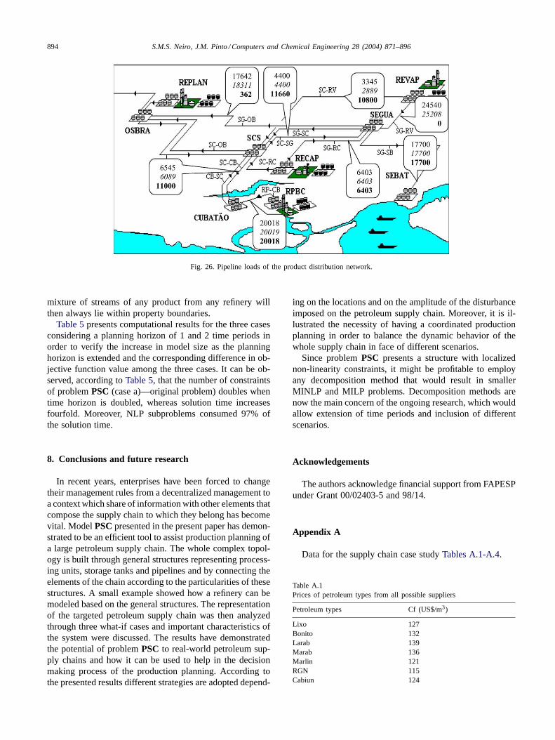
Indeed, distribution planning plays an important role byattempting to balance interferences suffered in the supplychain as observed how refineries react to the constraints im-posed on the system. Likewise, there is an impact on thedistribution facilities.Figs. 22–25show the percentage ofeach product transferred to terminals, whereasFig. 26showsthe total amount to be transported by each product pipelineaccording to the production planning. Again, the values innormal font in the callouts represent results for case (a) thevalues in italics represent results for case (b) and the val-ues in bold face represent results for the case (c). For case(b), it is observed that only little variations are established.For case (c), on the other hand, larger variations can be ob-served. Since all refineries are needed to satisfy the demandrequirements of the whole chain, products from refinery RE-

Fig. 23. Products feed flowrate percentage at terminal SCS.

VAP are then transferred to terminal SCS whereby transferis accomplished to other terminals. Moreover, product dis-tribution from the other refineries is significantly altered asseen byFigs. 22–25.

In terms of the objective function, case (a) presents netpresent value 0.5% higher than case (b) and 14% higher thancase (c).

As a conclusion for case (b), pre-selection of somepetroleum types tend to be counterbalanced by selectionof other petroleum types absorbing the disturbing effectat the refinery level. A comparison of the petroleum typeselections between case (a) and case (b) really revealsthat there is a great difference in terms of number andamount of petroleum types selected. Such a measure avoidspropagation of the disturbance over other facilities of thecomplex. As a conclusion for case (c), opposite to case (b),disturbance can only be absorbed by the whole distributionsystem.


Fig. 24. Products feed flowrate percentage at terminal CUBATAO.

7. Computational results

Non-linearity in problemPSC appears in constraints (2),(4), (12), (14), (38) and (44)–(47) and also the objectivefunction (18). Such equations represent process units orproduct tanks. Therefore, non-linearity is present only at re-finery models. Although terminal models are basically rep-

Table 5Computational results

Case (a) Case (b) Case (c)

Time period 1 Time period 2 Time period 1 Time period 2 Time period 1 Time period 2

Constraints 2304 4607 2306 4611 2304 4607Variables 2544 5087 2544 5087 2544 5087Discrete variables 195 390 195 390 195 390Solution time (CPU s) 116.8 656.2 152 915.6 157.8 2301.5

Fig. 25. Products feed flowrate percentage at terminal OSBRA.

resented by product tanks,Eq. (12)is not included in the setof constraints describing these tanks. Instead, product qual-ity constraints are applied at refinery product tanks. Productproperties must be within a range established by customerspecifications and environmental regulations. Once all re-fineries are subjected to the same quality constraints, thereis no need to recalculate properties at terminals, since


Fig. 26. Pipeline loads of the product distribution network.

mixture of streams of any product from any refinery willthen always lie within property boundaries.

Table 5presents computational results for the three casesconsidering a planning horizon of 1 and 2 time periods inorder to verify the increase in model size as the planninghorizon is extended and the corresponding difference in ob-jective function value among the three cases. It can be ob-served, according toTable 5, that the number of constraintsof problemPSC (case a)—original problem) doubles whentime horizon is doubled, whereas solution time increasesfourfold. Moreover, NLP subproblems consumed 97% ofthe solution time.

8. Conclusions and future research

In recent years, enterprises have been forced to changetheir management rules from a decentralized management toa context which share of information with other elements thatcompose the supply chain to which they belong has becomevital. ModelPSC presented in the present paper has demon-strated to be an efficient tool to assist production planning ofa large petroleum supply chain. The whole complex topol-ogy is built through general structures representing process-ing units, storage tanks and pipelines and by connecting theelements of the chain according to the particularities of thesestructures. A small example showed how a refinery can bemodeled based on the general structures. The representationof the targeted petroleum supply chain was then analyzedthrough three what-if cases and important characteristics ofthe system were discussed. The results have demonstratedthe potential of problemPSC to real-world petroleum sup-ply chains and how it can be used to help in the decisionmaking process of the production planning. According tothe presented results different strategies are adopted depend-

ing on the locations and on the amplitude of the disturbanceimposed on the petroleum supply chain. Moreover, it is il-lustrated the necessity of having a coordinated productionplanning in order to balance the dynamic behavior of thewhole supply chain in face of different scenarios.

Since problemPSC presents a structure with localizednon-linearity constraints, it might be profitable to employany decomposition method that would result in smallerMINLP and MILP problems. Decomposition methods arenow the main concern of the ongoing research, which wouldallow extension of time periods and inclusion of differentscenarios.

Acknowledgements

The authors acknowledge financial support from FAPESPunder Grant 00/02403-5 and 98/14.

Appendix A

Data for the supply chain case studyTables A.1-A.4.

Table A.1Prices of petroleum types from all possible suppliers

Petroleum types Cf (US$/m3)

Lixo 127Bonito 132Larab 139Marab 136Marlin 121RGN 115Cabiun 124


Table A.1 (Continued )

Petroleum types Cf (US$/m3)

Albaco 117Bicudo 123Condoso 118Bonit 127Bonny 132Marli 121RGNE 121Cabiuna 115Albacor 124Brass 115Palanca 124Larabe 118Coso 127

Table A.2Inventory costs at every facility

Tank type Cinv (US$/m3 d)

Petroleum Product

SEBAT 0.11 –SEGUA 0.23 0.35SCS – 0.28CUBATAO 0.25 0.27OSBRA – 0.46REVAP 0.12 0.32RPBC 0.12 0.32RECAP 0.12 0.32REPLAN 0.12 0.32

Table A.3Transportation costs for petroleum and product pipelines

Petroleum pipeline Ct (US$/m3) Product pipeline Ct (US$/m3)

OBT-I 0.044 SG–SB 0.098OBT-II 0.044 SG–RV 0.031OVT-I 0.052 SG–SC 0.037OVT-II 0.038 SG–OB 0.024OVT-III 0.045 SG–RC 0.036

SC–RV 0.051SC–RC 0.085SC–OB 0.049SC–SG 0.037SC–CB 0.042RP–CB 0.034OB–SC 0.032CB–SC 0.042

Table A.4Product sale prices and demands for refineries, terminals and pipelines

Refinery REVAP Refinery RPBC

Cp(US$/m3)

Dem(m3)

Cp(US$/m3)

Dem(m3)

PC3 180 500 PGLP 118 200PC4 100 100 PDIN 230 350PMTBE 100 0 PDME 242 500

Table A.4 (Continued )

Refinery REVAP Refinery RPBC

Cp(US$/m3)

Dem(m3)

Cp(US$/m3)

Dem(m3)

PGLP 115 130 PDMA 212 300PJFUEL 130 200 PNAP 146 900PPQN 148 600 PNAT 160 158PGLN 149 1000 PPGC 152 600PDIN 210 500 POC 180 1500PDME 230 600 PDO 159 700PDMA 206 200 PGLN 270 500PFO1A 139 800 PGLA 290 500PFO1B 142 50 PGLE 298 200PFO4A 151 4000 PXIL 160 100PEXFO 146 300 PTOL 167 45

PBEN 280 210

RECAP REPLAN

PDIN 132 0 PNAL 128 330PGLP 65 200 PNAP 151 3850PRAT 98 500 PJFUEL 175 100PGC 202 400 PDIL 150 0POCP 144 90 PMTU 180 200PLCO 0 400 PGLN 181 2000PGLN 141 150 PGLP 215 400PSOLB 231 300 PPGC 122 230PDILT 236 200 PDIN 280 2000POCBV 257 90 PDMA 267 500

PDME 254 6000PFO1A 160 1050PFO1B 162 1500PFO4A 158 2800PEXFO 149 990

Terminal SEBAT CUBATAO OSBRA

Cp(US$/m3)

Dem(m3)

Cp(US$/m3)

Dem(m3)

Cp(US$/m3)

Dem(m3)

PDIN 230 3000 230 4000 230 10500PDME 242 4400 242 3000 242 5500PDMA 226 3000 226 2000 226 5400PGLN 270 6500 270 600 270 1000PJFUEL 175 0 175 200 175 500PGLP 128 800 128 800 128 3600

References

Barnes, R., Linke, P. & Kokossis, A. (2002). Optimization of oilfield development production capacity. InESCAPE 12 proceedings(pp. 631–636). The Hague, the Netherlands.

Beamon, B. M. (1998). Supply chain design and analysis: models andmethods.International Journal on Production Economics, 55, 281–294.

Bok, J. K., Lee, H., & Park, S. (1998). Robust investment model forlong-range capacity expansion of chemical processing networks un-der uncertain demand forecast scenarios.Computers and ChemicalEngineering, 22(7–8), 1037–1049.

Bok, J. K., Grossmann, I. E., & Park, S. (2000). Supply chain optimizationin continuous flexible processes.Industrial and Engineering ChemistryResearch, 39, 1279–1290.

Brooke, A., Kendrick, D. & Meeraus, A. (1998).GAMS: a user’s guide.San Francisco, CA: The Scientific Press.

Cheng, L. & Duran, M. (2003). World-wide crude transportation logistics:a decision support system based on simulation and optimization. In


I. E. Grossmann & C. M. McDonald (Eds.),Proceedings of fourthinternational conference on foundations of computer-aided processoperations (pp. 273–280). Coral Springs, CAChE.

Dempster, M. A. H., Pedron, N. H., Medova, E. A., Scott, J. E., &Sembos, A. (2000). Planning logistics operations in the oil industry.Journal of Operational Research Society, 51(11), 1271–1288.

Drud, A. S. (1994). CONOPT: a large scale GRG code.ORSA Journalof Computing, 6, 207–216.

Escudero, L. F., Quintana, F. J., & Salmeron, J. (1999). CORO, a model-ing and an algorithmic framework for oil supply, transformation anddistribution optimization under uncertainty.European Journal of Op-erational Research, 114(3), 638–656.

Feord, D., Jakeman, C. & Shah, N. (2002) Modeling multi-site pro-duction to optimize customer orders. InESCAPE 12 proceedings(pp. 661–666). The Hague, the Netherlands.

Forrest, J. & Oettli, M. (2003). Rigorous simulation supports accuraterefinery decisions. In I. E. Grossmann & C. M. McDonald (Eds.),Proceedings of fourth international conference on foundations ofcomputers-aided process operations (pp. 273–280), Coral Springs,CAChE.

Iakovou, E. T. (2001). An interactive multiobjective model for the strategictransportation of petroleum products: risk analysis and routing.SafetyScience, 39, 19–29.

IBM (1991). OSL, guide and reference (release 2). Kingston, NY: IBM.Ierapetritou, M. G., Floudas, C. A., Vasantharajan, S., & Cullick, A. S.

(1999). Optimal location of vertical wells: decomposition approach.AIChE Journal, 45(4), 844–859.

Iyer, R. R., Grossmann, I. E., Vasantharajan, S., & Cullick, A. S. (1998).Optimal planning and scheduling of offshore oil field infrastructureinvestment and operations.Industrial and Engineering Chemistry Re-search, 37, 1380–1397.

Jia, Z. & Ierapetritou, M. (2003). Efficient short-term scheduling ofrefinery operations based on a continuous time formulation. In I.E. Grossmann & C. M. McDonald (Eds.),Proceedings of fourthinternational conference on foundations of computer-aided processoperations (pp. 327–330), Coral Springs, CAChE.

Kosmidis, V. D., Perkins, J. D., Pistikopoulos, E. N. (2002). A mixedinteger optimization strategy for integrated gas/oil production. InES-CAPE 12 proceedings (pp. 697–702), The Hague, the Netherlands.

Lamming, R. (1996). Squaring lean supply chain management.Inter-national Journal of Operation and Production Management, 16(2),183–196.

Lasschuit, W. & Thijssen, N. (2003). Supporting supply chain planningand scheduling decisions in the oil & chemical industry. In I. E.Grossmann & C. M. McDonald (Eds.),Proceedings of fourth inter-national conference on foundations of computer-aided process oper-ations (pp. 37–44), Coral Springs, CAChE.

Lee, H., Pinto, J. M., Grossmann, I. E., & Park, S. (1996). Mixed-integerlinear programming model for refinery short-term scheduling of crudeoil unloading with inventory management.Industrial and EngineeringChemistry Research, 35(5), 1630–1641.

Liu, M. L., & Sahinidis, N. V. (1997). Process planning in a fuzzyenvironment.European Journal of Operational Research, 100, 142–169.

Magalhães, M.V. & Shah, N. (2003). Crude oil scheduling. In I. E.Grossmann & C. M. McDonald (Eds.),Proceedings of fourth inter-national conference on foundations of computer-aided process oper-ations (pp. 323–326), Coral Springs, CAChE, 323–326.

Magatão, L., Arruda, L. V. R., Neves-Jr, F. (2002). A mixed integerprogramming approach for scheduling commodities in a pipeline. InESCAPE 12 proceedings (pp. 715–720), The Hague, the Netherlands.

Más, R., & Pinto, J. M. (2003). A Mixed-Integer Optimization Strategy forOil Supply in Distribution Complexes.Optimization and Engineering,4, 23–64.

Perea, E., Grossmann, I. E., Ydstie, B. E., & Tahmassebi, T. (2000).Dynamic modeling and classical control theory for supply chain

management.Computers and Chemical Engineering, 24, 1143–1149.

Perea-López, E., Grossmann, I. E., & Ydstie, B. E. (2001). Dynamicmodeling and decentralized control of supply chains.Industrial andEngineering Chemistry Research, 40, 3369–3383.

Pinto, J. M., & Moro, L. F. L. (2000). A planning model for petroleumrefineries.Brazilian Journal of Chemical Engineering, 17(4–7), 575–585.

Pinto, J. M., Joly, M., & Moro, L. F. L. (2000). Planning and schedulingmodels for refinery operations.Computers and Chemical Engineering,24, 2259–2276.

Ponnambalam, K., Vannelli, A., & Woo, S. (1992). An interior pointmethod implementation for solving large planning problems in the oilrefinery industry.Canadian Journal of Chemical Engineering, 70(2),368–374.

Ross, A. D. (2000). Performance-based strategic resource allocation insupply networks.International Journal of Production Economics, 63,255–266.

Sear, T. N. (1993). Logistics planning in the downstream oil industry.Journal of Operational Research Society, 44(1), 9–17.

Song, J., Bok, J. K., Park, H. & Park, S. (2002). Supply chain optimiza-tion involving long-term decision-making.ESCAPE 12 proceedings(pp. 799–804). The Hague, the Netherlands.

Stebel, S. L., Arruda, L. V. R., Fabro, J. A., Rodrigues L.C.A. (2002).Modeling liquefied petroleum gas storage and distribution.ESCAPE12 proceedings (pp. 805–810). The Hague, the Netherlands.

Tan, K. C. (2001). A framework of supply chain management litera-ture.European Journal of Purchasing and Supply Management, 7, 39–48.

Thomas, D. J., & Griffin, P. M. (1996). Coordinated supply chain man-agement.European Journal of Operational Research, 94, 1–15.

Türkay, M., & Grossmann, I. E. (1996). Logic-based MINLP algorithmsfor the optimal synthesis of process networks.Computers and Chem-ical Engineering, 20, 959–978.

Van den Heever, S. A., & Grossmann, I. E. (1999). Disjunctive multiperiodoptimization methods for design and planning of chemical processsystems.Computers and Chemical Engineering, 23, 1075–1095.

Van den Heever, S. A., & Grossmann, I. E. (2000). An iterative ag-gregation/disaggregation approach for the solution of a mixed-integernonlinear oilfield infrastructure planning model.Industrial and Engi-neering Chemistry Research, 39, 1955–1971.

Van den Heever, S., Grossmann, I. E., Vasantharajan, S., & Edwards, K.(2000). Integrating complex economic objectives with the design andplanning of offshore oilfield infrastructure.Computers and ChemicalEngineering, 24, 1049–1055.

Vecchietti, A., & Grossmann, I. E. (2000). Modeling issues and imple-mentation of language for disjunctive programming.Computers andChemical Engineering, 24, 2143–2155.

Vidal, C. J., & Goetschalckx, M. (1997). Strategic production-distributionmodels: a critical review with emphasis on global supply chain models.European Journal of Operational Research, 98, 1–18.

Viswanathan, J., & Grossmann, I. E. (1990). A combined penalty functionand outer-approximation method for MINLP optimization.Computersand Chemical Engineering, 14, 769.

Wenkai, L. & Hui, C. W. (2003). Plant-wide scheduling and marginalvalue analysis for a refinery. In I. E. Grossmann & C. M. McDonald(Eds.),Proceedings of fourth international conference on foundationsof computer-aided process operations (pp. 339–342). Coral Springs,CAChE.

Ydstie, B. E., Coffey, D. & Read, M. (2003). Control and optimiza-tion of supply networks. In: I. E. Grossmann, C. M. McDonald(Eds.),Proceedings of fourth international conference on foundationsof computer-aided process operations (pp. 167–185). Coral Springs,CAChE.

Zhuo, Z., Cheng, S., & Hua, B. (2000). Supply chain optimization ofcontinuous process industries with sustainability considerations.Com-puters and Chemical Engineering, 24, 1151–1158.

Documents

A general modeling framework for the operational …cepac.cheme.cmu.edu/pasilectures/pinto/revpaper-NP.pdf · Computers and Chemical Engineering 28 (2004) 871–896 A general modeling