A General Introduction to RAM - ProAIM Ltd · Introduction to RAM ... represent the logic relationships between component failures ... data input into an RBD/FT, engineers will be

Process Asset Integration & Management (Trading as ProAIM) Ltd

One Central Park, Northampton Road, Manchester, M40 5BP, UK

T. +44 (0)161 918 6790

E. [email protected] www.proaimltd.com

Introduction to RAM

What is RAM?

RAM refers to Reliability, Availability and Maintainability. Reliability is the

probability of survival after the unit/system operates for a certain period of

time (e.g. a unit has a 95% probability of survival after 8000 hours). Reliability

defines the failure frequency and determines the uptime patterns.

Maintainability describes how soon the unit/system can be repaired, which

determines the downtime patterns. Availability is the percentage of uptime

over the time horizon, and is determined by reliability and maintainability.

Why choose RAM Analysis?

RAM has a direct impact on profit through lost production and maintenance

costs. The main objectives of RAM are to increase system productivity, increase

the overall profit as well as reduce the total life cycle cost — which includes lost

production cost, maintenance cost, operating cost, etc.

Some significant figures are:

As much as $100,000 per hour typical production losses can be sustained

in base chemical plants due to non-availability

In oil refineries, production losses are millions of dollars per year for every

1% of non-availability

In oil refineries, the maintenance staff are up to 30% of total manpower

Maintenance spending is one of the largest parts of the operational budget

after energy and raw material costs

Each year over $300 billion is spent on plant maintenance and operations

by US industry, and it is estimated that approximately 80% of this is spent

on systems and people to correct the unplanned failure of machines

(Engineering Maintenance, 2002)

The operation and maintenance budget request of the US Department of

Defence for the fiscal year 1997 was on the order of $79 billion



T. +44 (0)161 918 6790


RAM analysis is essential to the system profitability. Even small improvements

in the effectiveness of RAM schemes make large additions to the bottom line.

Role of RAM Analysis

Fig.1 illustrates the interactions and applications of RAM analysis. For an

existing process, maintenance data are usually recorded in the CMMS

(Computerised Maintenance Management System). These data can be analysed

through qualitative and quantitative approaches, as shown in Fig.2.

Fig.1 RAM Analysis Cycle

Failure Analysis (Qualitative & Quantitative)

RBD or Fault Tree

Maintenance Strategy

Optimisation

Process Synthesis or

Retrofit

Improve Equipment

Design

Stocking Policy Optimisation

Basic Analysis – Equipment

Basic Analysis – System

Applications

Operation Stage Design Stage



T. +44 (0)161 918 6790


Fig. 2 Failure Analysis

Failure mode and distribution parameters can be obtained for each unit in the

system. Reliability Block Diagrams (RBD) or Fault Trees (FT) can be used to

represent the logic relationships between component failures and system

failures, and provide the basis for a RAM study. With the failure distribution

data input into an RBD/FT, engineers will be able to understand the RAM

performances of the current system and carry on further developments and

optimisations. In fact, there is a direct relationship between RBD and FT, but

most engineers find RBD easier to use, as it can be more easily related to a

process flowsheet. The approach to RAM analysis adopted by Process

Integration Limited exploits RBDs.

In the operation stage, RAM analysis can be implemented to optimise

maintenance strategy as well as stocking policy for spare parts. The

maintenance strategy will then affect the failure records in the CMMS, which in

turn help engineers revise the maintenance strategy through time. New failure

records will be saved in the CMMS during the operating stage.

In the design stage, RAM analysis can be integrated into the design of the

system configuration, which will ensure the optimum design with balanced

RAM performance and total investment. Moreover, the qualitative and

quantitative analysis of process unit failures can help designers to modify the

structure of a specific process unit to improve the process design.

Failure Analysis

Distribution Parameters Regression

Failure Mode and Effect Analysis

(FMEA)

Qualitative Analysis Quantitative Analysis



T. +44 (0)161 918 6790


RAM analysis run throughout both operating and design phases to enable the

process to achieve high profitability.

Benefits of RAM Analysis

The following benefits can be obtained from RAM analysis.

Decision making

What maintenance policy should be applied

Investment decisions on maintenance

Resource utilisation

Inspection intervals

Optimum spare part purchasing

Appropriate maintenance scheduling

Understanding the financial implications of maintenance

Decision making based on modelling

Cost management

Managing the cost related to unavailability

Cost of maintenance

Etc.

Integration with other business activities

All projects on a site have an effect on process RAM

RAM needs to involve the whole organization

Meeting the business demand

Reduce outages caused by breakdowns

Reduce the loss of revenues caused by unavailability

Etc.

RAM Analysis Tools

There are several tools to conduct RAM analysis in different stages and for

different purposes, as shown in Figure 3.



T. +44 (0)161 918 6790


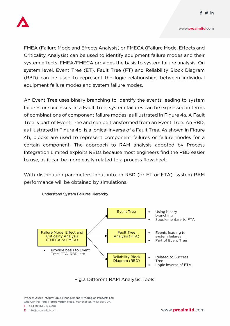
FMEA (Failure Mode and Effects Analysis) or FMECA (Failure Mode, Effects and

Criticality Analysis) can be used to identify equipment failure modes and their

system effects. FMEA/FMECA provides the basis to system failure analysis. On

system level, Event Tree (ET), Fault Tree (FT) and Reliability Block Diagram

(RBD) can be used to represent the logic relationships between individual

equipment failure modes and system failure modes.

An Event Tree uses binary branching to identify the events leading to system

failures or successes. In a Fault Tree, system failures can be expressed in terms

of combinations of component failure modes, as illustrated in Figure 4a. A Fault

Tree is part of Event Tree and can be transformed from an Event Tree. An RBD,

as illustrated in Figure 4b, is a logical inverse of a Fault Tree. As shown in Figure

4b, blocks are used to represent component failures or failure modes for a

certain component. The approach to RAM analysis adopted by Process

Integration Limited exploits RBDs because most engineers find the RBD easier

to use, as it can be more easily related to a process flowsheet.

With distribution parameters input into an RBD (or ET or FTA), system RAM

performance will be obtained by simulations.

Fig.3 Different RAM Analysis Tools

Reliability Block Diagram (RBD)

Fault Tree Analysis (FTA)

Failure Mode, Effect and Criticality Analysis (FMECA or FMEA)

Provide basis to Event Tree, FTA, RBD, etc

Understand System Failures Hierarchy

Event Tree Using binary branching

Supplementary to FTA

Events leading to system failures

Part of Event Tree

Related to Success Tree

Logic inverse of FTA



T. +44 (0)161 918 6790


a) Fault Tree b) Reliability Block Diagram

Fig.4 Fault Tree and Reliability Block Diagram Examples

Deterministic or Probabilistic Modelling

A RAM study is conducted through a probabilistic approach, which is

fundamentally different from a deterministic approach. The difference is

illustrated by an example. As shown in Table.1, 41 failures are recorded in 20

years. Table.2 lists other necessary data.

Table.1 Failure Records

Failure Record

No Time No Time No Time

1 02/05/1990 15 03/04/1996 29 28/01/2002

2 29/05/1990 16 20/10/1996 30 20/09/2002

3 07/07/1990 17 19/09/1997 31 23/05/2003

4 19/11/1990 18 02/09/1998 32 31/01/2004

5 07/04/1991 19 07/02/1999 33 19/10/2004

6 04/09/1991 20 22/07/1999 34 08/07/2005

7 04/02/1992 21 11/01/2000 35 08/04/2006

8 11/07/1992 22 11/04/2000 36 09/01/2007

9 28/01/1993 23 14/07/2000 37 04/11/2007

10 03/09/1993 24 22/10/2000 38 15/09/2008

11 13/04/1994 25 11/05/2001 39 07/01/2009

12 30/11/1994 26 04/07/2001 40 10/05/2009

13 03/04/1995 27 30/08/2001 41 21/05/2010

14 26/09/1995 28 12/11/2001



T. +44 (0)161 918 6790


Table.2 Maintenance and Cost Data

Mean Time To Repair (days) 5

Mean Time of PM (days) 1

CM Cost (K$ per action) 10

PM Cost (K$ per action) 2

Lost Production Cost

(K$/day) 240

Maintenance costs in Table.2 are associated with the penalties of consequent

damages to other units.

a) Deterministic Approach

According to the data in Table.1, Mean Time Between Failure (MTBF) = 7142

day/ 40 = 178 day. Using a deterministic approach, it is assumed the component

will fail every 178 days, as shown in Fig.5.

Fig.5 Failure Analysis using Deterministic Approach

To reduce unexpected failures, two preventive overhaul schemes are

considered:

1. Preventive overhaul at MTBF – 178 days

2. Using rule of thumb: preventive overhaul at 80% of MTBF – 145 days

Based on the economic data, total annual costs with different maintenance

policies are listed in Table.3. The cost comprises corrective maintenance cost,

preventive maintenance cost and lost production cost. As a result, preventive

Time

Up

178 day 178 day 178 day



T. +44 (0)161 918 6790


overhaul at MTBF reduces the cost by 19%. If rule of thumb is applied and

overhaul at 80% of MTBF, the total cost is reduced by 23%.

But it is dangerous to use the rule of thumb for every unit, since each unit has

different failure distribution patterns as well as different maintenance cost,

associated penalty cost, etc. It is not possible to find a “golden rule” which can

be applied for all of the process units. Costs could even be increased with a

wrong rule.

Table.3 Total Cost of Different Policy

Maintenance Policy Annual Cost (K$) Cost Reduced (%) Availability

No Preventive Overhaul 2421 Base 0.9726

Preventive Overhaul at MTBF 1960 19.04 0.9778

Overhaul at 80% MTBF 1848 23.67 0.9790

b) Probabilistic Approach

Using a probabilistic approach, the failures are represented by a probability

distribution. The Reliability curve and Probability Density Function curve are

shown in Fig.6. From this:

The probability that the component will fail in 60 days is 10%.




The component will fail most likely around 140 days, although MTBF is 178 days.

This indicates that the component is more likely to fail after 140 days.



T. +44 (0)161 918 6790


a) Reliability vs Time b) Probability Density Function

Fig.6 Reliability and Probability Density Function Curve

The frequency of preventive maintenance can be optimised based on economic

data. The results of such an optimization are listed in Table.4. Optimum

preventive interval is 105 days.

Table.4 Total Cost of Different Policy

Maintenance Policy Annual Cost (K$) Cost Reduced (%) Availability

No Preventive Overhaul 2421 Base 0.9726

Preventive Overhaul at MTBF

1960 19.04 0.9778

Overhaul at 80% MTBF 1848 23.67 0.9790

Overhaul at Optimal Interval

1767 27.01 0.9800

Cost optimisation using a probabilistic approach saves more money compared

with the deterministic approach. Inappropriate preventive overhaul scheme can

be avoided.

Redundancy Optimisation

Using standby components (sometimes referred to as spare or redundant

components) is a common way to increase system availability and profit in the

design stage, or even in retrofit. In addition to the inclusion of standby

equipment, the standby equipment can be exploited in different ways. Instead

Reliability

0

0.1

0.2

0.3

0.4

0.5

0.6

0.7

0.8

0.9

1

0 100 200 300 400 500 600 700 800

Time(day)

Reliab

ilit

y

Probability Density Function

0

0.0005

0.001

0.0015

0.002

0.0025

0.003

0.0035

0.004

0.0045

0.005

0 100 200 300 400 500 600 700 800

Time (days)

Pro

bab

ilit

y



T. +44 (0)161 918 6790


of having one item of equipment on line and vulnerable to breakdown, there

may be two, with one on-line and one off-line. But these two items of

equipment can be sized and operated in many ways:

2 x 100% one on-line, one off-line switched off

2 x 100% one on-line, one off-line idling

2 x 50% both on-line, with system capacity reduced to 50% if one fails

2 x 75% both on-line operating at 2/3 capacity when both operating, but

with system capacity 75% if one fails

Etc., etc.

Since different units have different availability features and capital costs,

engineers usually face difficulties to identify the optimum process structure –

which unit should have redundancy, how many standby items are required,

what is their capacity and what is their operating policy? Many factors should

be considered when making decisions, e.g. availability target, investment

budget, etc. Engineers need a systematic way to make decisions. Combining

reliability analysis with optimization allows redundancy to be optimised with

different objectives and constraints.

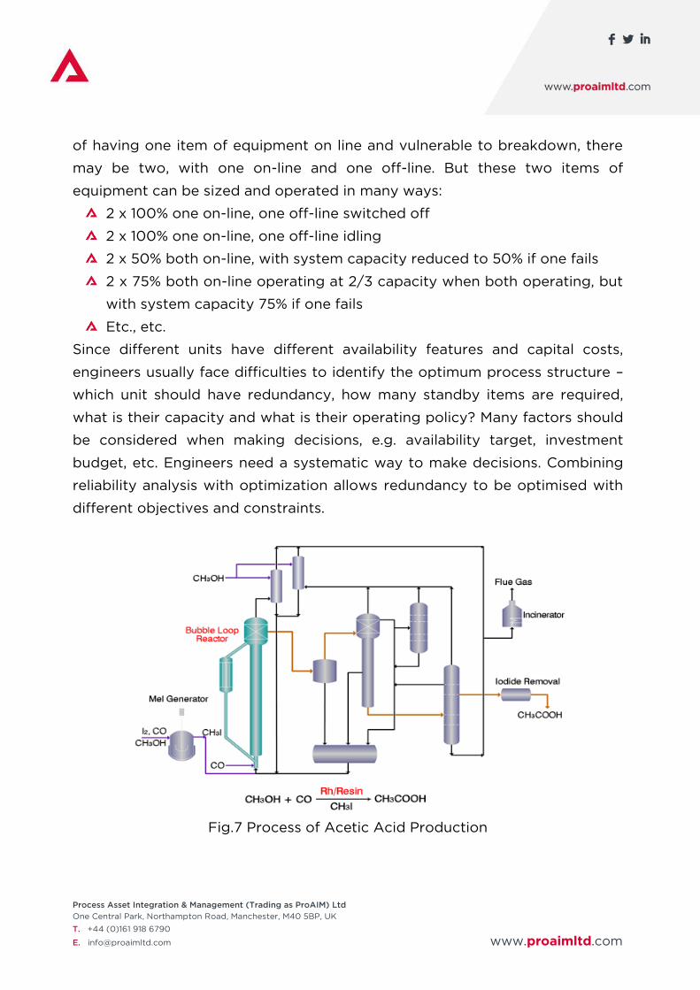
Fig.7 Process of Acetic Acid Production



T. +44 (0)161 918 6790


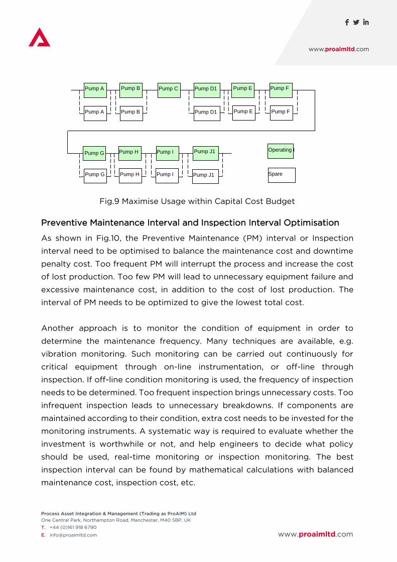
Using Fig.7 as an example, standby pumps are required for the acetic acid

production process. Pump data are listed in Table 5. Fig.8 and Fig.9 show two

different designs. Fig.8 is to minimise the total capital cost with the availability

target as 0.97. Pump D and Pump J are 2x50%, Pump E and G do not have

standby, all the others are 2x100%. Fig.9 maximises system usage within a

capital budget of 3.6x104 K$. Pump C does not have standby; all other pumps

are 2x100%.

A mathematical tool can help engineers make the best decisions on a sound

basis.

Table.5 Basic Information of Pumps

Pump ID Capacity

(%)

MTBF

(operation)

(days)

MTBF

(standby)

(days)

MTTR

(days) Availability

Capital Cost

(K$)

Pump A 100% 300 4000 4 0.9868 320

Pump B 100% 300 4000 5 0.9836 628

Pump C 100% 200 2000 10 0.9524 8000

Pump D1 100% 220 4000 10 0.9565 4660

Pump D2 75% 220 4000 8 0.9649 4200

Pump D3 50% 250 4000 8 0.9690 3600

Pump E 100% 330 4000 4 0.9880 1116

Pump F 100% 280 4000 5 0.9825 176

Pump G 100% 300 4000 4 0.9868 1316

Pump H 100% 290 4000 4 0.9864 676

Pump I 100% 300 4000 4 0.9868 820

Pump J1 100% 310 4000 4 0.9873 504

Pump J2 75% 330 4000 4 0.9880 450

Pump J3 50% 350 4000 4 0.9887 390

Fig.8 Minimise Capital Cost with Availability Target

Pump A

Pump D3

Pump J3

Pump A Pump B Pump C Pump E Pump F

Pump G Pump H Pump I

Pump B Pump C Pump F Pump D3

Pump H Pump I Pump J3

Operating I

Spare



T. +44 (0)161 918 6790


Fig.9 Maximise Usage within Capital Cost Budget

Preventive Maintenance Interval and Inspection Interval Optimisation

As shown in Fig.10, the Preventive Maintenance (PM) interval or Inspection

interval need to be optimised to balance the maintenance cost and downtime

penalty cost. Too frequent PM will interrupt the process and increase the cost

of lost production. Too few PM will lead to unnecessary equipment failure and

excessive maintenance cost, in addition to the cost of lost production. The

interval of PM needs to be optimized to give the lowest total cost.

Another approach is to monitor the condition of equipment in order to

determine the maintenance frequency. Many techniques are available, e.g.

vibration monitoring. Such monitoring can be carried out continuously for

critical equipment through on-line instrumentation, or off-line through

inspection. If off-line condition monitoring is used, the frequency of inspection

needs to be determined. Too frequent inspection brings unnecessary costs. Too

infrequent inspection leads to unnecessary breakdowns. If components are

maintained according to their condition, extra cost needs to be invested for the

monitoring instruments. A systematic way is required to evaluate whether the

investment is worthwhile or not, and help engineers to decide what policy

should be used, real-time monitoring or inspection monitoring. The best

inspection interval can be found by mathematical calculations with balanced

maintenance cost, inspection cost, etc.

Pump A

Pump D1

Pump J1

Pump A Pump B Pump C Pump E Pump F

Pump G Pump H Pump I

Pump B Pump E Pump F Pump D1

Pump H Pump I Pump J1 Pump G

Operating I

Spare



T. +44 (0)161 918 6790


Fig.10 Cost vs PM Interval/ Inspection Interval

Spare Parts Optimisation

Spare parts need to be stocked in the warehouse in order that units can be

repaired in time if they fail unexpectedly, or for planned maintenance. The

holding cost and depreciation cost can be very high if too many parts are

stocked. But if not enough parts are stocked, delivery delay time could increase

system downtime and lead to extra penalty cost. Stocking policy should be

determined according to the failure patterns of the parts. Mathematic analysis

is necessary to find the best stocking policy and balance the stocking cost

(including depreciation cost) and downtime penalty cost, as shown in Fig.11.

Fig.11 Total Cost vs. Different Stocking Policies

Cost vs PM interval

1200

1300

1400

1500

1600

1700

1800

1900

2000

2100

2200

50 100 150 200PM interval (Days)

Co

st (

K$

)

60

70

80

90

100

No CBM Inspection/6

w eeks

Inspection/4

w eeks

Inspection/2

w eeks

Inspection/1

w eek

Real-time

Monitoring Cost (K$/yr)

Penalty Cost (K$/yr)

Maintenance Cost (K$/yr)

0

0.5

1

1.5

2

2.5

3

3.5

4

4.5

5

5/3 4/2 3/1 2/0

Max/Min Stocking No

Co

st

(K$/y

ear)

Downtime Penalty Cost

(K$/year)

Holding Cost (K$/year)

Purchase Cost (K$/year)



T. +44 (0)161 918 6790


Methodology

Functions Methodology

Data Regression Rank Regression, Maximum Likelihood

Estimation

RAM Simulation Monte Carlo Simulation

Redundancy Optimisation Markov Analysis with optimization

PM Optimisation Monte Carlo Simulation with optimisation

CBM Optimisation Monte Carlo Simulation with optimisation

Spare Parts Optimisation Monte Carlo Simulation with optimisation

Documents

A General Introduction to RAM - ProAIM Ltd · Introduction to RAM ... represent the logic relationships between component failures ... data input into an RBD/FT, engineers will be