Embed Size (px)
Citation preview

A General Approach to Electrical Vehicle Battery
Remanufacturing System Design
by
Xinran Liang
A dissertation submitted in partial fulfillment
of the requirements for the degree of
Doctor of Philosophy
(Mechanical Engineering)
In the University of Michigan
2018
Doctoral Committee:
Professor Jun Ni, Chair
Assistant Professor Xiaoning Jin
Professor Huei Peng
Associate Professor Siqian May Shen

ii
To my family
iii
ACKNOWLEDGEMENTS
My doctoral study was a long journey. Many people helped me along the
way. I would like to express my gratitude to my supervisor, Professor Jun Ni, for his
guidance. Without his continuous support, this work will not be possible. Special
thanks to Professor. Xiaoning Jin, the discussions with whom have generated
innovative ideas in my dissertation. Many thanks to Professor Yoram Koren, Professor
Jack Hu, Professor Huei Peng, Professor Siqian Shen, for spending their precious time
serving on my dissertation committee and qualify exam committee.
I am very grateful for the collaborative environment at the S. M. Wu
Manufacturing Research Center. Thanks to George Qiao, Dr. Seungchul Lee,
Dr.Shiming Duan, Dr. Peter Pan, Dr. Hao Yu, Dr. Li Xu, Dr. Xi Gu, Dr. Yangbing Lou,
Dr. Junyi Shui,and many other lab members , for their help and friendship.
.

iv
TABLE OF CONTENTS
DEDICATION……………………………………………………………… …….…ii
ACKNOWLEDGEMENTS ......................................................................................... iii
LIST OF TABLES ........................................................................................................ ix
LIST OF FIGURES ....................................................................................................... x
ABSTRACT ............................................................................................................... xiii
CHAPTER 1 Introduction.............................................................................................. 1
1.1 Motivation ............................................................................................................ 1
1.2 Remanufacturing .................................................................................................. 6
1.3 Research Issues .................................................................................................... 7
1.4 Research Objectives ........................................................................................... 13
1.5 Outline of the Dissertation ................................................................................. 15
CHAPTER 2 Forecasting Product Returns for Remanufacturing Systems ................. 17
2.1 Background ........................................................................................................ 17
2.2 Literature Review............................................................................................... 22
v
2.3 Forecasting of Product Return Quantity ............................................................ 24
Influence Factors ......................................................................................... 24
Sales Distribution, S(t) ................................................................................ 25
Product Breakdown Distribution, B(t) ........................................................ 27
Customer Return Function, C(t) ................................................................. 29
Return Quantity Forecasting in Continuous Case ....................................... 31
Return Quantity Forecasting in Discrete Form ........................................... 33
Numerical Examples ................................................................................... 34
Monte Carlo Simulation Verification .......................................................... 36
Properties of Predicted Return Function ..................................................... 38
2.4 Quality Forecasting of Returned Products ......................................................... 39
Quality Distribution, Q(t, x)........................................................................ 40
Convolution in 3D....................................................................................... 42
Numerical Examples ................................................................................... 43
Verification with Monte Carlo Simulation .................................................. 47
2.5 Conclusions and Future Work ............................................................................ 48
CHAPTER 3 Lifecycle Warranty Cost Estimation for Electric Vehicle Battery Using
an Age-Usage Based Degradation Model .................................................................... 50
3.1 Introduction ........................................................................................................ 50

vi
3.2 Modeling ............................................................................................................ 55
Warranty Process ......................................................................................... 55
Usage Rate .................................................................................................. 57
Reliability-Centered Battery Degradation Model ....................................... 60
Influence of Usage ...................................................................................... 64
Replacement and Repair ............................................................................. 65
Sales Prediction Model ............................................................................... 68
Simulation Model........................................................................................ 69
3.3 Numerical Case Study........................................................................................ 72
Parameters ................................................................................................... 72
Results ......................................................................................................... 73
Effects of Altering Battery Reliability and Warranty Period ...................... 77
Effects of Altering Costs ............................................................................. 84
Effects of Purchasing Time Function (Sales Prediction) ............................ 85
3.4 Conclusions ........................................................................................................ 86
CHAPTER 4 Remanufacturing Supply and Demand Matching For EV Battery Packs
...................................................................................................................................... 88
4.1 Introduction ........................................................................................................ 88
4.2 Remanufacturing ................................................................................................ 90
vii
4.3 Supply Side ........................................................................................................ 92
Overview ..................................................................................................... 92
Supply Variation Influential Factors ........................................................... 93
Remaining Useful Life (RUL) .................................................................. 102
Supply During Market Lifetime ................................................................ 102
Major Assumptions for the Supply Side ................................................... 104
4.4 Demand Side .................................................................................................... 105
Overview ................................................................................................... 106
Two Types of Demands ............................................................................. 106
Failure Types and Demanded Parts ........................................................... 107
Demand during Market Lifetime .............................................................. 109
Major Assumptions for the Demand Side ................................................. 110
4.5 Demand and Supply Matching......................................................................... 111
Overview ................................................................................................... 111
Repairing/Remanufacturing Policies ........................................................ 112
Warranty Policies ...................................................................................... 114
Inventory Policies ..................................................................................... 117
Optimization ............................................................................................. 119
Major Assumptions for Matching ............................................................. 121

viii
4.6 Conclusion ....................................................................................................... 122
CHAPTER 5 Conclusion and Future Work ............................................................... 123
5.1 Conclusion and Contributions ......................................................................... 123
5.2 Proposed Future Work ..................................................................................... 126
Bibliography .............................................................................................................. 128

ix
LIST OF TABLES
Table 1-1. Traditional manufacturing and remanufacturing comparisons ..................... 8
Table 3-1. Characteristics of different types of repairs. ............................................... 67
Table 3-2. List of parameters. ...................................................................................... 72
Table 3-3. Simulation results ....................................................................................... 73
Table 4-1. Simulated failure type composition before and after warranty period. .... 101
Table 4-2. Parts replacement and remanufacturing policy. ........................................ 107
Table 4-3. Failure and cost break down during market life by remanufacturing policy
types. .......................................................................................................................... 113
Table 4-4. Market life cost by different inventory policies. ....................................... 119
Table 4-5. Optimization results. ................................................................................. 121

x
LIST OF FIGURES
Figure 1-1. The "servitization" process (Oliva & Kallenberg, 2003) ............................ 4
Figure 1-2. Spectrum of different types of manufacturer-customer relationships ......... 5
Figure 1-3. Possible remanufacturing systems when different parties are included. ... 11
Figure 2-1. Remanufacturable products are the area supply and demand (for
illustration only) ........................................................................................................... 20
Figure 2-2. Customer return behavior distribution. ..................................................... 30
Figure 2-3. Relationship between sales, breakdown and return. ................................. 32
Figure 2-4. Return quantity forecasts........................................................................... 36
Figure 2-5. Analytical results (smooth curved) vs. Monte Carlo Simulation results
(step curves). ................................................................................................................ 37
Figure 2-6. Adding high frequency noise to S(t) results in overlapping R(t)'s. ........... 39
Figure 2-7. Sales distribution, S(t,x). ........................................................................... 43
Figure 2-8. Quality distribution, Q(t,x). ....................................................................... 44
Figure 2-9. Customer return distribution, C(t,x). ......................................................... 45
Figure 2-10. Return quantity and quality distribution, side view and top view........... 46
Figure 2-11. Monte Carlo for returned product quantity and quality. .......................... 48
Figure 3-1. Examples of battery degradation with high and low usage rates and age
limits. ........................................................................................................................... 57

xi
Figure 3-2. Usage rate distribution. ............................................................................. 59
Figure 3-3. Effective Warranty (EW) distribution where EW< 8 years (top) and the
entire EW distribution (bottom). .................................................................................. 60
Figure 3-4. Simulation of degradation processes with threshold = 20% ..................... 62
Figure 3-5. Failure functions for replacing, imperfect repair and minimal repair. ...... 66
Figure 3-6. Simplified flow chart of current practice for a single customer ................ 71
Figure 3-7. Histogram of lifecycle costs for (a) manufacturer, (b) customer. ............. 74
Figure 3-8. Probability density function of predicted sales using Bass diffusion model.
...................................................................................................................................... 75
Figure 3-9. Failure schedule for manufacturer for replacements, minimal repairs and
imperfect repairs. ......................................................................................................... 76
Figure 3-10. Cost Schedule for manufacturer. ............................................................. 77
Figure 3-11. Average cost paid by customers with varying warranty and breakdown
time. ............................................................................................................................. 79
Figure 3-12. Average cost paid by manufacturer with varying warranty and
breakdown time. ........................................................................................................... 80
Figure 3-13. Average total cost when warranty and reliability functions are varied. .. 81
Figure 3-14. Cost schedule when reliability remains constant and warranty changes. 82
Figure 3-15. Cost Schedule, constant reliability function, and warranty limit change in
small increments. ......................................................................................................... 83
Figure 3-16. Cost schedule when warranty is constant, altering reliability function. . 84
Figure 3-17. Changing in Sales distribution results virtually no change in costs. ....... 86

xii
Figure 4-1. Car life distribution. .................................................................................. 95
Figure 4-2. Distributions for pack electronics, frame/enclosure and module physical
failures.......................................................................................................................... 98
Figure 4-3. First failure date. ..................................................................................... 101
Figure 4-4. Supply during market life (3D view and top view)................................. 104
Figure 4-5. Demand during market lifetime (3D and top view). Both Return Date and
RUL are in months. .................................................................................................... 110
Figure 4-6. Distribution of driving profile scaler, D (top) and charging cycle per
month, C (bottom). ..................................................................................................... 116
Figure 4-7. Effects of changing total warranty charging cycles on supply and demand.
Both RUL and Date are in months. ............................................................................ 117
xiii
ABSTRACT
One of the major difficulties electrical vehicle (EV) industry facing today is
the production and lifetime cost of battery packs. Studies show that using
remanufactured batteries can dramatically lower the cost. The major difference
between remanufacturing and traditional manufacturing is the supply and demand
variabilities and uncertainties differences. The returned core for remanufacturing
operations (supply side) can vary considerably in terms of the time of returns and the
quality of returned products. On the other hand, because different contracts can be
used to regulate suppliers, it is almost always assumed zero uncertainty and variability
for traditional manufacturing systems. Similarly, customers demand traditional
manufacturers to sell newly produced products in constant high quality. But,
remanufacturers usually sell in aftermarket, and the quality of the products demanded
can vary depends on the price range, usage, customer segment and many other factors.
The key is to match supply and demand side variabilities so the overlapping between
them can be maximized. Because of these differences, a new framework is needed
for remanufacturing system design.
xiv
This research aims at developing a new approach to use remanufactured
battery packs to fulfill EV warranties and customer aftermarket demands and to match
supply and demand side variabilities. First, a market lifetime EV battery return
(supply side) forecasting method is develop, and it is validated using Monte Carlo
simulation. Second, a discrete event simulation method is developed to estimate EV
battery lifetime cost for both customer and manufacturer/remanufacturer. Third, a
new remanufacturing business model and a simulation framework are developed so
both the quality and quantity aspects of supply and demand can be altered and the
lifetime cost for both customer and manufacturer/remanufacturer can be minimized.
The business models and methodologies developed in this dissertation
provide managerial insights to benefit both the manufacturer/remanufacturer and
customers in EV industry. Many findings and methodologies can also be readily
used in other remanufacturing settings. The effectiveness of the proposed models is
illustrated and validated by case studies.
1
CHAPTER 1
CHAPTER 1
Introduction
1.1 Motivation
Energy and environment are two major social concerns today, and electrical
vehicles (EV) have enormous potential to positively impact their future. EVs also
become increasingly trendy in recent years. General Motors (GM) invested almost
half billion USD and thousands of engineers in 2014 for its next generation
“electrification” (GM, 2014). Similarly, Tesla, a growing leader in semi-
autonomous EVs, is fueled by US$4.9 billion of government’s subsidies (Hirsch,
2015). Almost all major automotive manufacturers are investing significant amount
of money and resources into the development, manufacturing, and marketing of EVs.
Despite this tremendous effort, the total number of EVs sold each year is still
insignificant compared to the sales of internal combustion engine (ICE) vehicles in
the U.S., at around only 1% of the total market share (EVVolumes, 2016).
Moreover, there are plenty of governmental incentives at the federal, state, and local
levels. For example, if a resident in Sonoma county, California purchases a new EV,
such as Nissan Leaf or Tesla Model S, he/she can receive $10,500 in incentive,
$7,000 from federal, $2,500 from state and $1,000 from the county (DriveClean,

2
2016). However, these heavy incentive programs have not been effective at bringing
sales up.
Among many factors contributing to this problem, high selling price is
arguably the most important factor from the customers’ perspective. In many cases,
lowering the price can boost sales dramatically. For instance, Forbes reported that
after Nissan lowered the price of its Leaf EV by US$6,000 in 2013, sales jumped 18%
(Dan Bigman, 2013). The high price problem is attributable to various factors, and
production cost is one of the main issues. Out of all the components in an EV, the
battery pack creates the greatest burden in cost. Although the exact cost for a battery
pack is confidential for most manufacturers, it is reported that a Nissan Leaf’s battery
pack costs as much as $18,000 to replace (Eric Loveday, 2010), and a Ford Focus EV
battery pack costs $12,000 to $15,000 apiece (or one third to one half of the car’s
cost) (Ramsey, 2012). The battery alone can cost as much as a compact car.
Within a battery pack, the most expensive components are the battery cells.
Argonne National Laboratory’s Center for Transportation provides a percentage
breakdown for manufacturing cost of an EV battery; 80% is battery cell and material
related (IJESD, 2000). It is estimated that it costs Tesla $195 per kWh and GM $215
kWh to produce their battery packs in 2016 (InsideEVs, 2016). Because of this high
cost, many manufacturers sell EVs at a loss. Fiat-Chrysler stated that every time a
Fiat 500e is sold, company losses $10,000 to $14,000 (P. Samaras, 2014; AutoWeek,
2011).
Moreover, battery packs usually cannot last for the entire lifespan of an EV,

3
so a second, or subsequent battery pack, is needed to continue using the vehicle.
Battery packs in current generation EVs can only last 6 to 8 years under the
engineering specifications for vehicle power batteries. However, the average
ownership of passenger vehicles is around 12 years. To resolve this issue, Nissan
introduced a $100-per-month battery replacement program for their Leaf EV (for 2nd
battery pack) in 2014. Although gasoline is not used, the sum of the initial purchase
cost and the life-cycle cost for EVs is actually significantly higher than an ICE car’s
cost of ownership. Currently, this circumstance is not an issue because the majority
of the EV batteries haven’t reached its end-of-life. In addition, to attract more
customers, original equipment manufacturers (OEMs) for EVs usually provide a
liberal warranty, even at a loss. In many cases, the battery warranty is sufficiently
long, such that, even if old battery degrades, a brand-new battery is given to customer
for free (at OEM’s cost) as replacement.
Furthermore, battery technology development cannot keep up with the
automotive industry. Even though some manufacturers, such as Tesla, claim that
battery cell’s price can go to $100 per kWh by 2025 (GreenTechMedia, 2016), the
battery pack for a Tesla Model S will still cost more than $22,000 to produce, if other
related electronics are included. On the other hand, a brand-new low trim Honda
Civic, a very popular small size sedan, only costs $16,000. Hence, OEMs are
desperately trying to lower the battery cost, and they cannot entirely depend on
technology improvements.
One way to solve this problem is to alter EV business models, such as

4
remanufacturing the battery packs. The business model used in both manufacturing
and auto industries has changed tremendously in the past decade. Manufacturing
and other heavy machinery industries are gradually shifting to a “servitization”
business strategy. Simply speaking, OEMs no longer sell products or machineries, but
are selling machine usage time. All other matters, such as maintenance, training,
sometimes even operation can be included as part of their service. (Oliva &
Kallenberg, 2003) described the servitization journey as a sequence of phases with
increasing service content as in Figure 1-1 ((Oliva & Kallenberg, 2003)). From
selling products to taking responsibility of the customer’s business, servitization
gradually changes the ownership and relationship between OEMs and customers.
Similarly, as Uber, Lyft and other car sharing companies become increasingly popular,
the definition of car ownership is also changing in the auto industry.
Figure 1-1. The "servitization" process (Oliva & Kallenberg, 2003)
In addition, EV OEMs, such as Tesla and many Chinese EV companies, are
also expanding their charge stations. Tesla is even building battery swapping stations.
This changes the interaction dynamics between EV OEMs and customers
dramatically. Auto manufacturers are shifting from no interaction with customers to
frequent interactions. As shown in Figure 1-2, as new business models develop, a

5
full spectrum of ownership types and interactions are coming into existence.
Figure 1-2. Spectrum of different types of manufacturer-customer relationships
As interactions become more frequent and ownership of the car becomes
more ambiguous (sharing between customers and OEMs), it is possible to create EV
power battery remanufacturing programs. In an early attempt Tesla built battery
swap stations in early 2016, their business model is still largely unknown, and other
business models have not matured enough for detail research. For this research, the
approach for establishing a battery remanufacturing program is considered and
focused on the repair-center level interactions.
It is estimated that battery remanufacturing costs 20% of the original cost to
manufacture (Jin, Hu, Ni, & Xiao, 2013), and remanufactured batteries can be used as
a sufficient battery replacement after the first battery retires. The intuition is very
straightforward: if battery warranty is 8 years and battery fails during the 7th year, the
manufacturer only needs to replace a battery that lasts for 1 year or longer. A new
battery that can last 7 or 8 years is excessive. Moreover, if a battery dies during the

6
9th year and the customer only wants to use the car for 12 years, this customer can buy
a battery replacement that can last for 3 years. He/she most likely does not want to
spend another $15,000 ~ $20,000 for a new battery replacement.
1.2 Remanufacturing
Remanufacturing may have different meanings in different industries. It is
usually defined as “an industrial process to recover value from the used and degraded
products to like-new’ condition by replacing components or reprocessing used
component parts” (Lund, 1984). In this dissertation, it is the process to reconstruct a
product, to certain specifications, from field returned used products and/or newly
manufactured components. One aspect that is different from other industries is that
the final remanufactured product may be a mixture of used and new parts. That is,
traditional suppliers are also part of the supply network, whereas many other
remanufacturing industries, such as tire and container remanufacturings, only use
returned parts as their supply.
In addition, remanufacturing and reuse of returned EV batteries are very
different from the simple waste recycling and remanufacturing. It requires a
systematic method to manage the used vehicle battery subsystems. The general
process of diagnosis, disassembly, testing, sorting, reassembly, and testing is more
complicated than most other remanufacturing processes. The importance of
sustainably managing large numbers of failed EV batteries with proper end-of-life
treatment has been recognized, but the fundamental research issues are still not well-

7
understood and systematic methodologies and challenges to solve the problems are
lacking (Jin, 2012).
Remanufacturing also provides economic incentives to firms by selling the
remanufactured products and extending the life cycles of products. Successful
examples from industry, such as BMW, Cummins, IBM, and Xerox, show that
remanufacturing can be profitable and there is a big market for the secondary use of
remanufactured products. According to the EPA, the estimated total annual sales of
73,000 remanufacturing firms in the United States were US$53 billion in 1997. The
fact that remanufacturing can be profitable has also been well documented (Ayres,
Ferrer, & Van Leynseele, 1997; Lund, 1983).
1.3 Research Issues
Currently, remanufacturing researches can be divided into three main fields:
designing, planning and processing. Designing primarily includes product design
and remanufacturing system design. System design can be further divided into
remanufacturing supply chain, facility, and process design. From business
perspective, designing also includes subjects such as pricing and remanufactured
product marketing. Planning contains market and return forecasting, process
sequencing, job sequencing, capacity planning, inventory management, uncertainty
management, product acquisition and so on. Processing mainly focuses on the
physical aspect of the operation, and it is comprised of disassembly, cleaning,
inspecting, sorting, re-assembly and many more. However, the structure of research

8
still follows the traditional approach used in manufacturing research.
In order to have a better understanding of the remanufacturing system, it is
important to understand what the major/fundamental differences between a traditional
manufacturing system and remanufacturing system are. These differences are
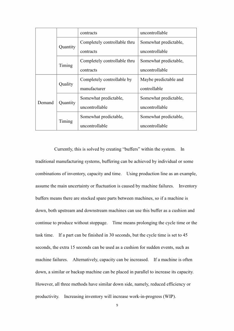
summarized in Table 1-1 and explained below.
From a system’s perspective, it is critical to determine the characteristics of
its inputs and outputs. Essentially, a system is only a mechanism to transfer
available inputs to desirable outputs. For traditional manufacturing systems, their
input or supply side is assumed to be completely predictable and controllable through
contracts with suppliers. For their demand side, or the output, only quantity and
timing are somewhat predictable or controllable; all other aspects are assumed to be
completely predictable and controllable. On the other hand, for a remanufacturing
system, its supply side or the cores/product returns are highly unpredictable and
uncontrollable in all aspects of quantity, quality and timing. Similarly, the quantity,
quality and time of its demand are also full of uncertainties and fluctuations.
Although remanufacturing has been studied and implemented for decades, this
fundamental challenge, namely matching supply side and demand side fluctuations
and uncertainties, is still largely untouched.
Table 1-1. Traditional manufacturing and remanufacturing comparisons
Traditional manufacturing Remanufacturing
Supply Quality Completely controllable thru Somewhat predictable,
9
contracts uncontrollable
Quantity Completely controllable thru
contracts
Somewhat predictable,
uncontrollable
Timing Completely controllable thru
contracts
Somewhat predictable,
uncontrollable
Demand
Quality Completely controllable by
manufacturer
Maybe predictable and
controllable
Quantity Somewhat predictable,
uncontrollable
Somewhat predictable,
uncontrollable
Timing Somewhat predictable,
uncontrollable
Somewhat predictable,
uncontrollable
Currently, this is solved by creating “buffers” within the system. In
traditional manufacturing systems, buffering can be achieved by individual or some
combinations of inventory, capacity and time. Using production line as an example,
assume the main uncertainty or fluctuation is caused by machine failures. Inventory
buffers means there are stocked spare parts between machines, so if a machine is
down, both upstream and downstream machines can use this buffer as a cushion and
continue to produce without stoppage. Time means prolonging the cycle time or the
task time. If a part can be finished in 30 seconds, but the cycle time is set to 45
seconds, the extra 15 seconds can be used as a cushion for sudden events, such as
machine failures. Alternatively, capacity can be increased. If a machine is often
down, a similar or backup machine can be placed in parallel to increase its capacity.
However, all three methods have similar down side, namely, reduced efficiency or
productivity. Increasing inventory will increase work-in-progress (WIP).

10
Increasing time will decrease efficiency. Increasing capacity will decrease utility.
Similarly, remanufacturing systems also implement “passive buffers”. In
addition, it also uses price as a buffer, such as the high profit margin in medical
devices, aerospace, electricity generators or large machineries. Because profit margin
is high, it is still profitable after 40 to 50% fluctuations. Therefore, in the context of
remanufacturing, high profit margin and small input/output fluctuation industries can
thrive. This observation is one of the main reasons remanufacturing flourishes in only
a handful of industries; both demand and supply are highly predictable or “buffers”
can easily be placed.
The purpose of this dissertation research is to explore alternative
possibilities besides creating “passive buffers”. It is well known in other
engineering disciplines, such as electrical, control and system engineering, that a
better way to cope with uncertainties and fluctuations from both the input and output
is to create a feedback loop. In this scenario, the traditional remanufacturing system
needs to be expanded. Therefore other elements, such as customers and the
manufacturing system, need to be included into the system under study.

11
Figure 1-3. Possible remanufacturing systems when different parties are included.
To create a closed loop as shown in Figure 1-3, customers need to be linked
with the remanufacturing system. The best way to link them is through business
contracts between remanufacturers and other manufactures. This is where the
“servitization” concept comes in. Although this is not yet widely implemented in
remanufacturing industry, it exists in small scale. For example, some printer OEMs
sign contracts with their large customers and guarantee the cartridge and toner usage
for certain period. During this time period, the return and supply of cartridges and
toner replacements can be regulated by the printer OEMs. Essentially, it creates a
12
“closed loop” between OEMs and customers.
The key of this research is to reduce both demand side and supply side
fluctuations and uncertainty by creating a similar “closed loop” between EV OEMs
and customers. To establish this loop, the traditional one-time contractual
relationship (car purchasing) needs to be extended to a lifelong relationship.
Luckily, modern EV OEMs, such as Tesla, also operate their own repair centers and
charge stations (gas station equivalent), and car warranties can be implemented,
similar to those used for printer cartridge/toner contracts. By implementing more
effective warranty and repair/remanufacturing policies, OEMs can better forecast
customers’ behavior and have a more predictable and controllable remanufacturing
system.
On the other hand, remanufacturing faces uncertainties and fluctuations in
both supply and demand sides. Unlike traditional manufacturing, quality can also be
different. Remanufacturing supply side is mainly dependent on returned core, or a
used product returned by customers. After certain period of usage, the product can
be worn and torn differently depending on customers, so all three attributes (timing,
quality and quantity) of the return are almost impossible to regulate compared to
traditional manufacturing. For the demand side, as illustrated by Chapter 4 of this
research, customers also demand different quality of products at different times. The
quality can be dependent on many factors, such as warranty period, usage, expected
product life-time, expected using time and many more.

13
Besides coping with uncertainty and fluctuations, there are other research
issues, such as battery degradation. Over the life of the battery, the battery may be
charged and discharged for hundreds or even thousands of cycles. As this occurs, the
individual energy storage cells may age differently. Cells may degrade at different
rates. If this phenomenon is not corrected, one or more cells may become
undercharged or overcharged, either of which can lead to accelerated degradation or
failure of the battery packs.
1.4 Research Objectives
To achieve the goal of matching supply side and demand side variability, this
study is divided into three stages. In first stage, a mathematical formulation is
derived and used to predict both the quality and quantity of return during the entire
market lifespan of the EV battery packs. In this stage, objectives can further be
divided into:
Determination of factors that affect returns
Integration of factors into a coherent formulation
Representation of the demand as a three-dimensional curve
Validation of the above formulation with simulation and numerical
examples
Matching the variables cannot be implemented in abstract, and it needs to be
considered in a business setting. For the remanufacturing of EV battery packs,

14
warranty fulfillment becomes the nature linkage between customers and OEMs.
Here, it is assumed the OEM is also the remanufacturer. For supply side, because of
warranty, OEM can obtain used battery packs from customers as packs are broken
down. For the demand side, in some situations, remanufactured packs can be used
as battery replacement to fulfill warranties. To simplify both the quality and
quantity dimensions of both supply side and demand side matching process, cost is
used. That is, parts with different qualities are translated to monetary values and are
matched by monetary terms. Thus, stage two is to determine different costs for both
customers and OEMs during both the individual lifespan of an EV car and the entire
market lifespan. In this stage, objectives are divided into the following tasks:
In addition to factors from stage one, determine how different factors
affect costs (e.g. warranty terms, repair types, and degradations).
Integrate all the factors using discrete event simulation (DES).
Determine the lifetime costs for customer and the OEM.
Determine the total market lifespan cost for the OEM
Determine the total market lifespan cost and cost schedule for the OEM
In stage three, everything from stages one and two are included. The
matching process essentially is to shift both the 3D demand and supply curves and to
change the shapes of these curves to maximize the overlapping area between them.
The objectives are divided into the following tasks:

15
In addition to the influential factors in stages one and two, determine
replacing/repairing schemes and inventory factors affecting return
Generate 3D demand and supply curves
Determine how different matching strategies can shift and change the
shapes of these curves
Maximize the overlap between supply and demand curves
1.5 Outline of the Dissertation
The rest of the dissertation is divided according to the three stages listed
above. In Chapter 2, only the supply of the remanufacturer is considered. Customers
are linked with OEMs through the warranty contract, and the main focus is to predict
the timing, quality and quantity of supply side or the battery return. For this study,
the EV sales distribution, battery breakdown distribution and customer return
distribution are studied. In Chapter 3, different costs are determined. Again,
OEMs are linked with customers through the warranty contract. The four types of
costs for the warranty are illustrated. Beside the influential factors listed in Chapter
2, warranty, usage rate and battery degradation are also studied. In Chapter 4, both
supply and demand sides are considered. All three parties: manufacturer, customer
and remanufacturer are included in the system. The focus is to match both input and
output uncertainties and fluctuations. For this study, manufacturer and
remanufacturer are considered to be one entity or the same firm, so all information

16
between them is transparent and all actions are synchronized. All influential factors
from both Chapters 2 and 3 are included. In addition, different
repair/remanufacturing schemes and inventory policies are also studied. Conclusion
is given in Chapter 5.
17
CHAPTER 2
CHAPTER 2
Forecasting Product Returns for Remanufacturing Systems
2.1 Background
As the global manufacturing environment becomes increasingly
competitive, more and more manufacturers view remanufacturing as an important
opportunity for profit generation. Remanufacturing provides a means for a society
to treat product life cycle from a more holistic perspective, offers an alternative to
traditional recycle and reuse, and increases resources utilization. Remanufacturing is
the process that recovers residual value from used or degraded products by
disassembly and recovery at module level or at component level. This is
accomplished by restoring used products to ‘like-new’ condition by replacing broken
or degraded components or by reprocessing used components (Sutherland, Adler,
Haapala, & Kumar, 2008; Lund, 1984). Focusing on value-added recovery is the
main difference between remanufacturing and other types of end-of-life (EOL)
treatments, such as recycling (Westkämper, Alting, & Arndt, 2001; Guide, 2000).
This is also the reason that remanufacturing systems are viewed and treated more
similar to traditional manufacturing systems than simple recycling.
18
Remanufacturing is a fast-growing industry. In the United States alone,
remanufacturing operations (excluding military) has a $53 billion per year market
share (Hauser & Lund, 2003), and it is growing from between 10% to above 50%,
depending on industry and product types (Sahay, Srivastava, & Srivastava, 2006).
Automotive Parts Remanufacturers Association estimated that the remanufactured
units were roughly 10 million in 1995, 15 million in 2000, 20 million in 2005, and 30
million in 2015 (Buxcey, 2003).
The variability of both supply and demand sides are the most critical issues
facing industry today. Many other remanufacturing topics, such as inventory
management, are designed to either isolate or mitigate these fluctuations. In a
survey (Hammond, Amezquita, & Bras, 1998), 43% of automotive part
remanufacturers considered that parts availability was the number one difficulty for
their operation, and 41.2% of them used the availability of parts as the main criterion
to decide whether or not to remanufacture a given product. A number of research
groups (Marx-Gomez, Rautenstrauch, Nürnberger, & Kruse, 2002; Guide, Jayaraman,
& Srivastava, 1999) stated that the uncertainty in time and amount was the single
most important factor that influenced remanufacturing system planning. Guide et al.
(2000) listed seven major problems that remanufacturing systems faced today, and
three of them were related to this problem. Uncertainty from supply side (returned
products) is the most crucial characteristic of remanufacturing problems, and it
distinguishes remanufacturing from traditional manufacturing systems. Unlike
traditional manufacturers, remanufacturers usually have less or no direct control of the

19
returned parts. Figure 2-1 illustrates an example of variations in both supply and
demand sides. From a remanufacturer’s perspective, supply is the volume of
returned used products, and demand is how many remanufactured products are
desired. The overlapping area denotes remanufacturable quantity when delays in
inventory, remanufacturing time, and other factors are neglected. As the figure
shows, remanufacturing operations are essentially matching processes that intend to
maximize the overlapping region under demand and supply curves, and in order to
match, forecasts of both supply and demand curves are necessary. Moreover, in
addition to the variations in quantity and arrival times, quality variation is equally
important since returned products can have a wide range of conditions, but finished
products usually need to meet the same quality specification. This poses a unique
problem that traditional manufacturing systems do not encounter, so new techniques
are needed to predict and actively change the shape of both supply and demand
curves. Preceding research have considered incentives, such as discount and
advertisements, into account to optimize the overall remanufacturable volume
(Ghoreishi, Jakiela, & Nekouzadeh, 2011). This study is more focused on the
prediction of the supply curve.

20
Figure 2-1. Remanufacturable products are the area supply and demand (for illustration only)
There exists a spectrum of remanufacturing scenarios, which have very
different types of return characteristics. For example, the return process of leased
printer is very predictable since the return date and/or quality are predefined by the
leasing contracts. However, the return characteristics of many fashionable goods and
consumer electronics are more random since the sales of the items, usage pattern, and
customer return behavior are all unpredictable. Because of this variation in
predictability, different forecasting approaches are required for different business
settings. This research targets the recently developed electrical vehicle (EV) battery
return applications. The urgency and importance of EV battery remanufacturing is
because of limited and costly resources, the modular nature of lithium batteries, and
potential resale market. Current lithium ion (Li-ion) battery-powered vehicles, such as
Chevy Volt and Nissan Leaf, whose batteries are warranted for 8–10 years or
100,000–150,000 miles, are likely to fail before the expected life of the vehicles. The
returned battery may still have significant residual value. The cost of Li-ion battery is
still very high, usually around US$200 per kWh. Therefore, remanufacturing has great
potential to dramatically reduce the total life-cycle costs of Li-ion batteries (Jin et al.,
21
2013; Jin, Ni, & Koren, 2011). Industries also propose different types of
purchase/warranty schemes in order to allow customers to have operational batteries
for the entire vehicle lifespan. That is, customers are now able to purchase not only a
single battery pack with the EV but also the warranty of battery use-time, or the
combination of them. In this type of business scenario, broken or degraded batteries
can be returned or traded in to dealers or battery collectors and be replaced with a new
battery before the predefined total use-time expires. The new batteries can then be
made with components from returned batteries. This creates strong incentives for
customers to return the battery and for manufacturers to remanufacture. Since this
business scenario is completely new, the goal of this research is to develop a long-
term forecasting method to remanufacturers and related suppliers to assist their
operational decisions.
The challenges for forecasting of product returns are mainly from two
sources: lack of quality/credible data and unproven assumptions. There is no or very
limited historical data since this type of remanufacturing business scenario has never
been seen in the industry, and data is also limited or of low accuracy/credibility in
similar fields. These challenges seriously limit the type of forecasting techniques that
can be implemented. With these constraints, a physical model-based forecasting
method, instead of traditional data-driven methods that heavily rely on data quality
and sophisticated statistical models, is proposed here.
The objective of this research is to provide a methodology to forecast both
quantity and quality of returned products, such as EV batteries, based on

22
previous/expert knowledge on indirect information rather than direct historical data.
The rest of this chapter is organized as follows. Literature review highlights previous
literature regarding remanufacturing return forecasting. The final section summarizes
this research work and points out possible future research directions.
2.2 Literature Review
Although sales forecasting has been studied for many decades, there are few
scientific papers regarding return item forecasting for remanufacturers, and the
majority of them are focused on short-term tactical and operation level mainly for
inventory management and production planning (Guide & Wassenhove, 2003). For
some scenarios, simple classical forecasting techniques, such as moving average and
exponential smoothing, are sufficient (Nahmias & Cheng, 1993). However, often,
there is more valuable information that people can take advantage of, and a variety of
forecast outputs are required for different situations (Toktay, van der Laan, & de
Brito, 2004). Therefore, specific techniques are developed to tailor to those specific
needs. In some cases, periodical information, such as monthly volume, is available
and the need is to predict the future volume (Clottey, Benton, & Srivastava, 2012).
In other cases, historical return dates are available and other characteristics, such as
return lead times, are predicted. Kelle and Silver (Kelle & Silver, 1989) developed
four different forecasting methods for expected value and variance of return lead
times of containers. Goh and Varaprasad (Goh & Varaprasad, 1986) used a transfer
function model that included factors, such as previous returns, sales, and time lag, to
23
predict the timing and quantity of returns of Coca-Cola bottles. Toktay et al.
(Toktay, Wein, & Zenios, 2000) developed a Bayesian estimation-based distributed
lag model, which used newly collected data to update estimated parameters. As
listed above, the majority of existing studies use a statistics-based method for
prediction with historical data.
Other types of forecasting methods that include previous knowledge,
simulation, or known sub-models are often used. Marx-Gomez et al. (2002) combined
simulation and fuzzy logic models to forecast the quantities and timing of returns of
photocopiers. Simulation was used to obtain sales, failures, usage intensity, return
quotas, and other so-called impact factors. Then, fuzzy controller was used to
combine these impact factors and give one-period prognosis and neuro-fuzzy network
was used to provide multi-period prognosis. Similarly, Hanafi et al. (Hanafi, Kara,
& Kaebernick, 2007) used fuzzy-colored petri nets to combine different sub-models,
such as technology development, consumer demands, and product reliability to
forecast returns at different locations over a specific time period. For others, non-
parametric models are more suitable. For example, Monte Carlo simulation can be
employed to estimate the sale of products, such as CRT televisions. The gap between
existing literature and our current need is that the above methods are used for
prognosis and for relatively short-term prediction but not for lifespan planning of the
business or facility. Furthermore, the existing literature has not addressed much on the
quality variation of returned products, which is critical for battery remanufacturing.
To fill the gap in the existing literature, this research develops a new forecasting tool
24
for end-of-life product returns in terms of timing, quantity, and quality to support the
remanufacturing strategic planning and decision making.
2.3 Forecasting of product return quantity
Quantity forecasts provide information on how many product returns a
remanufacturer can expect in the future. However, unlike most forecasts that only
deal with a one-time customer decision, such as buying or not buying, returning is
determined by a series of cascaded events, i.e., product purchase decision, product
usage, and product return decision. In this section, a new method is presented for
predicting product returns. The key is to effectively characterize three main
influencing factors—sales, life expectancy, and return behavior—to facilitate an
accurate forecasting of return timing, quantity, and quality. More specifically, the
reasons of product return considered in this research are limited to the failure-induced
return and end-of-life return. Other factors, such as the product technology
upgrading, may be reasons for why a customer returns a product, but are not
considered in this work.
Influence Factors
The three influential factors are date sold, usage, and return behavior, which
are related to OEM, the product, and customer respectively.

25
Sales Distribution, S(t)
Sales forecasting has been studied for many decades, and many
manufacturers, or third-party consultants, usually have their own forecasting models.
Moreover, it is common in industry that a non-analytical form of modeling is used.
This is because people tend to focus more on market research perspective of the
forecast. Techniques, such as concept test, focus groups, perceptual mapping,
conjoint analysis, and consumer clinics, are more often seen, in order to have a better
understanding of the customers’ preference and to adjust future plans. For example,
the information acceleration (IA) methods are used for GM’s electric vehicle sales
prediction (Urban, Weinberg, & Hauser, 1996). On the other hand, academic
researchers are more interested in mathematics-orientated approaches because they
can provide a more direct relationship among different influential factors. For this
reason, this research provides both analytical and numerical methods in order to
accommodate current industry practice.
For analytical-based forecasts, there are generally two categories:
aggregated and disaggregated models. For aggregated or top-down approaches, only
the cumulated behavior of a group of people is studied. On the other hand,
disaggregated or bottom-up models study individual decision makers that underlie
market demand or supply and integrate them. Although the emphasis in forecasting
and econometrics has generally shifted from aggregated to disaggregated models in
the past decades, most forecasting models people use in industry today are still of
aggregated form simply due to the difficulty and expense of collecting data on

26
individual consumers. Out of all aggregated models, Bass diffusion model is the
most often used (Mahajan, Muller, & Bass, 1995).
Diffusion of products or innovation is the theory that seeks to explain how,
why, and at what rate a new idea spreads through societies. The parameter that
characterizes this process is called the rate of adoption, and it is defined as the relative
speed in which members of a social system adopt an innovation. This rate is usually
measured by the length of time required for a certain percentage of the members to
adopt. Customers can be divided into many categories, such as innovators, early
adopters, early majority, late majority, and laggards. Groups are different in how
they perceive different innovation factors, such as relative advantage, compatibility,
and complexity of the product. Bass diffusion model is chosen because it has all the
essentials of diffusion models and yet is the most simplified and intuitive version. In
this model, only two customer groups, early adopters and followers, are considered.
The sales only include the originally manufactured products and the remanufactured
products are only used for warranty repair but not for original sale.
Mathematically, we use the following differential equation to represent the
Bass diffusion
( )( )
1 ( )
f tp qF t
F t
, (2-1)
where F(t) is the base function, and f(t) is the rate of change or derivative of F(t). p is
the coefficient of early adopters, advertising effect, or innovators in Bass’s original
27
model. It describes how quickly early adaptors are willing to purchase or to enter a
new market. q is the coefficient of followers, internal influence, word-of-mouth effect,
or imitator factors in the original model. Sales volume at time t, S(t), is the rate of
change of installed base f(t) multiplied by the market potential, m, and has the form of
( ) ( )St mf t . (2-2)
The solution to Equation (2-1) is
2
2
( ) exp( ( ( ) ) )( )
(1 exp( ( ( ) ) ) )
wher e t he t i me of peak sal es t i s:
l n l n
t
t
p q p qSt m
qp p qp
q pt
p q
. (2-3)
In practice, p and q are set equal since early adopters usually act much quicker than
followers. The choice of p and q depends on many other social factors and industry
(Lilien & Rangaswamy, 2004).
Product Breakdown Distribution, B(t)
Battery life expectancy is the degree of quality degradation during the usage
stage. Currently, battery condition monitoring typically refers to the evaluation of
battery state of charge (SOC), or the state of health (SOH). SOC is defined as the

28
amount of remaining charge in a battery before a recharge is required, and SOH is the
potential chargeable capacity of a battery compared to the original unused one. For
EV batteries, customers return a battery pack when certain degradation criteria are
reached, such as when SOC drops below 75% ~85%. Therefore, the return time
prediction is usually to predict the duration that a battery can last until the
manufacturer’s predefined threshold is reached.
The conventional approach for life expectancy prediction is to model
product condition or degradation by an appropriately chosen random process, and the
occurrence of failure or reaching of certain threshold is usually modeled as a Poisson
process. Weibull distribution is chosen for this study because its failure rate function
is only current state dependent. The system condition, or degradation state, is
modeled by a Brownian motion with positive drift. Under this assumption, the time
to failure corresponds to the first passage time of the Brownian motion and follows an
inverse Gaussian distribution. Weibull distribution is well studied for reliability
engineering, and reference can be found in many textbooks, i.e., (Rinne, 2008).
Weibull distribution is one of the solutions that assume the degradation
process is deterministic. The probability density function g(t), the hazard function
h(t), and cumulative distribution function G(t) of Weibull distribution are:
29
1
1
( | , , ) ( ) exp
( | , , )
( | , , ) 1 exp
wher e ; ; ,
c c
c
c
c t a t ag t a b c Bt
b b b
c t ah t a b c
b b
t aGt a b c
b
t a a b c
¡ ¡
. (2-4)
Here, the breakdown function B(t) is exactly the probability density function, i.e.,
B(t) = g(t) (Lilien & Rangaswamy, 2004). By changing the shape parameter, the
failure rate h(t) can be changed directly. It can be increasing, constant, or decreasing
over time. Piecewise curve fitting is commonly used to model the classic bell curve
for failure rate (Sharif & Islam, 1980; Pinder, Wiener, & Smith, 1978).
Customer Return Function, C(t)
The warning indicator of a battery failure is usually signaled on the
dashboard of an EV, very similar to maintenance reminder signals. Additionally,
similar to the maintenance behavior, people usually do not bring back the vehicle for
battery treatments immediately upon observing the warning signal. This is probably
due to the fact that the vehicle is still perfectly drivable and usually no noticeable
changes are detected. Another reason is that SOC or SOH aspects of the battery
usually degrade very gradually over a period of years without noticeable abrupt
changes.
People usually do not return immediately, and sometimes the time delay

30
between product failure and the return action can be as long as a year. The return
function is usually heavily skewed to the left as illustrated in Figure 2-2. This long-
tailed distribution indicates that the majority of people will return damaged or
unwanted product in a short period of time. However, there are also a considerable
amount of people who will return after a relatively long period of time. This kind of
characteristics can be modeled by inverse Gaussian functions due to its skewness,
positive support, and relatively easy expression (see Figure 2-2). Choosing inverse
Gaussian is also because its flexibility in modeling the following three characteristics:
(1) the majority of people return within certain time period, (2) only a small portion of
them return whenever they found convenient, and (3) the rest will never return.
Figure 2-2. Customer return behavior distribution.
Inverse Gaussian functions have the general probability distribution

31
function of
1/ 2 2
3 2
( )( ) exp ; , 0
2 2
i i t jCt i j
t j t
, (2-5)
where j >0 is the mean and i >0 is the shape parameter. C(t) represents the probability
that the customer returns the battery t time units after its failure.
Although there are many other factors that may influence the quantity and
quality of the returned products, such as government regulations, they are either not
appropriate for the EV battery return in North America or not proven to have
significant influence on return quantity or quality. Therefore, the three main factors
listed above are the focus in this study.
Return Quantity Forecasting in Continuous Case
As illustrated in Figure 2-3, the return quantity at any point in time, such as
at point R, is the summation of different sale quantity and product life expectancy
combination. That is, returned product at R may be purchased at time S1 and used for
B1 years, or purchased at time S2 and used for B2 years, and so on.
32
Figure 2-3. Relationship between sales, breakdown and return.
One way to characterize the relationship of these three influential factors is
to use convolution. Convolution for two continuous functions f(t) and g(t) is defined
as
( ) ( ) ( ) ( ) ( ) ( )
, : 0,
f t g t f g t d f t g d
f g
¡
.
(2-6)
For this problem, the volume of broken products at time t can be represented as the
convolution of the sales volume S(t) and the breakdown probability B(t). Then, the
total volume of product returns at time t, R(t) is the convolution of the consumer
return behavior C(t) and the previous convolution result S(t)*B(t) as follows:
( ) ( ) ( ) ( )Rt St Bt Ct (2-7)

33
where R(t) denotes the return quantity at time t, S(t) is the probability function of sales
quantity, B(t) is the probability function of breakdown time, and C(t) is the probability
function of customer return. Note that B(t) and C(t) may not be normalized to unity.
The integration of B(t) is less than unity because not all batteries are degraded to
certain threshold during the lifespan of an electric vehicle. The integration of C(t) is
less than unity because not all failed batteries are returned. Some customers may
choose not to return or return to third party collectors.
However, due to the complexity of the functions S(t), B(t), and C(t), there is
no closed-form solution for the convolution. Because only a finite range is needed,
these functions can be approximated over this desired range by some polynomial
functions. The coefficients of the polynomial are chosen such that the weighted
error between the approximation and original function is minimized in a least squares
sense. For example,
2 3
0 1 2 3
2
( ) . . .
wher e ar g mi n ( ( ) ( , ) )b
i i
a
St t t t
Rt Rt dt
%.
(2-8)
Return Quantity Forecasting in Discrete Form
As mentioned, most forecasting models used in industry are not analytical-
based, but are most likely produced and derived from different forms of marketing
research. Periodical, such as monthly or yearly, data instead of equation form of
S(t), B(t), and C(t) are provided. The advantage of using a discrete form is that the

34
raw data from reliability tests can be used directly without fitting into a model first.
Similar to continuous convolution, a discrete form of convolution can be defined as
1 1[ ] [ ] [ ] [ ] [ ] [ ]
m m
f n g n f n g n m f n mg nl l
, (2-9)
where both f[n] and g[n] have finite positive support, and l is a scale factor that is
related to number of samples for both f[n] and g[n] and is used for normalization.
Due to the simplicity of discrete convolution computation, many continuous functions
are first discretized then are taken convolution in discrete domain. Thus, no
symbolic integral of continuous functions is needed.
Numerical Examples
This section uses a numerical example to demonstrate the modeling
procedure. The sales volume of battery packs is the same as the sales volume of the
electric vehicles. A typical EV model usually has a market life of three to four years.
Hence, it is reasonable to assume 95% of the Bass diffusion function to be in the
range of [0, 4]. Substituting p =0.08, q =2, and m =1 into Equation (2-3), we obtain
S(t) and its polynomial approximation S˜(t) as follows:
2. 08
2. 08 2
5 4 3 2
( ) 54. 08(1 25 )
( ) 0. 011 0. 101 0. 511 1. 373 1. 631 0. 3952
t
t
eSt
e
S t t t t t T
%
.
(2-10)

35
Note that all the approximations in this section are over interval [0, 10] or ten years.
Ten-year is chosen so that it is well beyond average auto sales time of 6 to 8 years.
For breakdown function B(t), it is assumed that batteries are in the ”wear-
out zone” in around three to four years. Failures most likely occur around the sixth
year of its usage. Therefore, we have the following B(t) in the form of Weibull
distribution:
4
3
( / 2)
6 5 4 2
3. 5( ) 2
2
( ) 0. 005 0. 046 0. 249 1. 007 0. 588 0. 089
ttB t e
B t t t t t t
%
.
(2-11)
For return behavior, assuming μ = 0.5 and λ = 0.2, we have the following return
function
2
2
1/ 2 0. 2( 0. 5)
2* 0. 52
6 5 3 2
0. 2( )
2
( ) 0. 017 0. 151 0. 749 2. 233 0. 117 1. 409
t
tCt et
Ct t t t t t
%
(2-12)
Substituting into Equation (2-7), the resulting polynomial approximation of the return
function R(t) is obtained:
6 5 3 2( ) 0. 001 0. 074 0. 045 118 0. 086 0. 0084Rt t t t t t % . (2-13)

36
The result is shown in Figure 2-4.
Figure 2-4. Return quantity forecasts.
Monte Carlo Simulation Verification
Another way to predict the quantity of returned products is using a Monte
Carlo simulation. Monte Carlo simulation is a family of computational algorithms
that rely on repeated random sampling in order to obtain the final results. Assume
that the total number of customers be 100,000, thus 100,000 samples will be used.
For each sample, its sale date, expected product life, and customer returns are
generated according to the functions S(t), B(t), and C(t), respectively. For sales date,
it follows the Bass diffusion model as in previous sections. Technically speaking, it
is not strictly a probability distribution since the integration of the function may not

37
add to unity. Therefore, normalization is needed before sampling. For each sample,
the deterministic calculation is then calculated:
Return_date = sale_date + product_life + return_delay
For aggregation, a histogram is used to obtain the distribution of sale date,
product life, return delay, and return date, as illustrated in Figure 2-5.
Figure 2-5. Analytical results (smooth curved) vs. Monte Carlo Simulation results (step
curves).
To compare the results from Monte Carlo simulation with analytical results, the
difference between two curves is measured by an f-divergence method. One of the f-
divergence methods, KL-divergence value, is 0.028, and Hellinger distance is 0.035,

38
which are all much less than unity. These calculations indicate the results obtained by
both methods are very close to each other.
Properties of Predicted Return Function
Because of convolution and the general shapes of S(t), B(t), and C(t), the
operation acts like a weighted moving average. This moving average can also be
viewed as a “low-pass” finite impulse response filter. This means that only low
frequency information will be preserved, and high frequency information will be
eliminated by convolution. Here, the frequency of a function roughly means how
many times a function varies in a given time interval. By taking Laplace transform in
the continuous case or Z-transform in the discrete case, it can be shown that
distributions used by S(t), B(t), and C(t) are essentially low-pass filters (S. W. Smith,
1997). As a result, R(t) is smoothed by each distribution, and any small noises found
in S(t), B(t), or C(t) will be reduced. Figure 2-6 demonstrates a case where seasonality
noise (a sine function), or high frequency function, is added to the sales function, S(t).
Sine function is chosen because it contains only a single frequency.
( ) (1 0. 3 si n( 8 ) ) ( )noi sy
S t t S t , (2-14)
where t is in radians. Please note that the sine function has much higher frequency
than the original function. Also note that after the sine function is added, the mean,
variance and the area under the curve of S(t) is preserved. The resulting function R(t)

39
is the same before and after adding this seasonality noise component (see Figure 2-6).
Due to this smoothing effect, R(t) is not sensitive to high-frequency changes in S(t),
B(t), or C(t).
Figure 2-6. Adding high frequency noise to S(t) results in overlapping R(t)'s.
2.4 Quality Forecasting of Returned Products
Besides the quantity of the returned products, their quality is another critical
factor that production planners would like to know prior to remanufacturing planning.
In this study, the return product quality is defined as the remaining useful life (RUL)
of the unbroken parts of a returned product. A typical EV battery pack usually
consists of hundreds of battery cells. When the performance measurement of a
battery pack, such as SOC or capacity, drops below certain threshold, only one or a

40
few cells fail or degrade to unacceptable condition while the majority of the cells is
still in good or reasonable quality. Because not all the cells degrade at the same rate,
it is critical to estimate the RUL of good cells, so the remaining value can be assessed.
RUL is essentially a conditional probability distribution that determines how long it
takes to reach a certain threshold given that the battery cells have already survived a
certain amount of time (the time for the battery pack reaching the threshold). .
Three-dimensional plots are used to express the quality and quantity information as a
function of battery return date. The x-axis represents the battery return date, the y-
axis is the expected quality indicated by remaining life, and z-axis is the quantity
distribution.
Quality Distribution, Q(t, x)
Remaining useful life (RUL) is defined as a conditional random variable
Xt = T − t when T > t, where t is the time where a part has survived so far, and T is the
time to failure. The conditional reliability function Rt(t) contains all the information
required for RUL. The reliability function is defined as:
( ) Pr ( | ) ; , ,
Pr ( ) Pr ( ) 1 ( )( )
Pr ( ) 1 ( )
t
t
R x T t x T t t x T
T t x T t F TR x
T t F T
¡
.
(2-15)
From Equation (2-15), the failure rate of RUL Q(t, x) is then

41
( )( ) ( ) ( ) ( )
1 ( )t t t
f tf x R x h t x R x
x F t
,
(2-16)
and
( , ) ( , ) ( | ) ( ) ( ) ( ) ( )t t t
Qt x f t x f x t f t h t x R x f t , (2-17)
where x = T − t, and f(t), F(t), and h(t) are time to failure probability density function
(pdf), cumulative distribution function (cdf), and hazard rate functions defined
previously. The conditional distribution becomes:
exp
( )
exp
c
t c
t x a
bR x
t a
b
,
(2-18)
and the joint probability then becomes:
1
1
1 12
2
( , ) exp
exp
exp
c c c
c c
c c c
c t x a t a t x aQt x
b b b b
c t a t a
b b b
c t x a t a t x a
b b bb
.
(2-19)

42
Convolution in 3D
It is assumed that the quality is uniform when the product is initially
shipped out of the factory or at the time of purchase, so the third dimension of S(t) is
invariant. So we have S(t, x) = S(t). Similarly, because consumer’s behavior will not
be affected by the RUL of returned battery, their return behavior would not be affected
by return time either, i.e., C(t, x) = C(t). Because of this invariance in both S(t, x) and
C(t, x), the convolution is only performed in one dimension, and it is independent of
the ‘quality’ dimension. That means
( , ) ( , ) ( , ) ( , )
( , ) ( , )
, : 0,
f t g t f x g t x dx
f t x g t dx
f g
¡
.
(2-20)
The final result of R(t, x) is the one-dimensional convolution of S(t, x), Q(t, x), and
C(t, x):
( , ) ( , ) * ( , ) * ( , )Rt x St x Qt x Ct x . (2-21)

43
Numerical Examples
2.4.3.1 Sales distribution, S( t, x)
Continuing the numerical example from Section 2.3.4 and the sales function
are essentially the same as Equation (2-18). The 3D shape of the function is shown in
Figure 2-7. It is constant in the quality direction because it is assumed the newly
sold battery packs all have the same high quality. Note that the cross section is the
same as the two-dimensional S(t), and it is peaked around 2 years.
Figure 2-7. Sales distribution, S(t,x).
2.4.3.2 Quality distribution, Q(t, x)
The quality distribution is determined by two factors: the product

44
breakdown time t and RUL x. The relationship is given by Q(t, x) for this example.
The shorter the product usage time t is, the longer the expected RUL x is, as in Figure
2-8. Because the mode of breakdown function Q(t, x) along the t direction is around 7,
the quality of returned product decreases dramatically towards zero. The peak
occurs when quality is zero because majority of the cells in a battery pack is at low
quality state when return.
Figure 2-8. Quality distribution, Q(t,x).
2.4.3.3 Customer return distribution, C( t, x)
Similar to the sales function, the customer return behavior function is also
constant along the quality axis since return behavior would not alter the quality of the
product itself. That is, C(t, x) = C(t), which is shown in Figure 2-9.
45
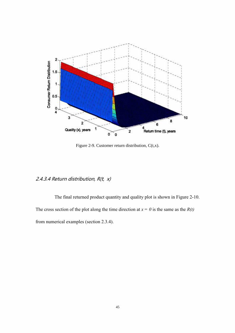
Figure 2-9. Customer return distribution, C(t,x).
2.4.3.4 Return distribution, R(t, x)
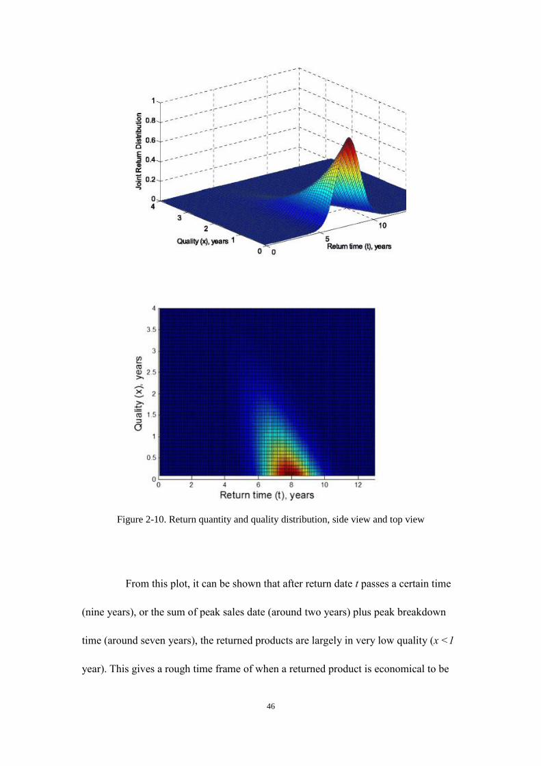
The final returned product quantity and quality plot is shown in Figure 2-10.
The cross section of the plot along the time direction at x = 0 is the same as the R(t)
from numerical examples (section 2.3.4).
46
Figure 2-10. Return quantity and quality distribution, side view and top view
From this plot, it can be shown that after return date t passes a certain time
(nine years), or the sum of peak sales date (around two years) plus peak breakdown
time (around seven years), the returned products are largely in very low quality (x <1
year). This gives a rough time frame of when a returned product is economical to be
47
remanufactured. Some other end-of-life treatment, such as recycling or proper
disposal, may be employed after certain time.
Verification with Monte Carlo Simulation
For this illustrative example, one million samples are used for each of the
random input generation. The generation of the sales date, expected product life, and
customer return behavior is the same as in the Monte Carlo simulation verification.
The RUL of returned products is generated by randomly drawing samples from Q(t, x)
where t of each sample is determined by the expected product life samples. Therefore,
whenever a sample is generated, the Q(t, x) distribution needs to be recalculated. As
before, Q(t, x) is not normalized, so it needs to first be discretized then normalized for
each sample.
Each sample has two components: the return date and return quality. Return
date is calculated in the same way as in the Monte Carlo simulation verification. The
return quality is sampled directly from Q(t, x) as shown in the previous subsection.
The distribution is obtained by using two-dimensional histogram or other scientific
volume imaging techniques. The simulation results shown in Figure 2-11 agree well
with R(t, x) obtained using the proposed analytical convolution-based approach.

48
Figure 2-11. Monte Carlo for returned product quantity and quality.
2.5 Conclusions and Future Work
This research provides a methodology to forecast long-term trend of both
quantity and quality of product returns, or the supply to a remanufacturing system, by
modeling three major influential factors (i.e., sales, life expectancy, and customer
return behavior) and their combinatory formulation in a forecasting method. To meet
the emerging needs of decision support in the remanufacturing industry, reliable
forecasting of supply can help determine a reasonable estimate of used products
attainable under a given set of conditions and further assist decision-makings in
remanufacturing operations. The effectiveness and accuracy of the forecasting model
developed in this research is verified and validated with the Monte Carlo simulations.
Generally, the typical goals of strategic forecasting are threefold: (1)
estimate the opportunity and outcome for future business activities, (2) find what
influence and how to influence outcome, and (3) judge the potential risks associated
with such business actives. The first two are covered by this research. The model

49
developed in this research only provides the most likely outcome based on a single set
of assumptions, so potential risks are more difficult to discover. Future works may
include sensitivity analysis, scenario analysis, and different assumption management
techniques.
50
CHAPTER 3
CHAPTER 3
Lifecycle Warranty Cost Estimation for Electric Vehicle Battery
Using an Age-Usage Based Degradation Model
3.1 Introduction
With the Honda Insight hybrid being the first electric mass production car
sold in the United States in 1999, electric vehicles (EVs) have grown steadily in the
US. Both technology and consumer acceptance progressed significantly over the last
decades. However, the sales of EVs have not been as optimistic as people originally
thought. In President Obama’s 2011 State of the Union Address, he called for
putting one million of EVs on the road by 2015 (Voelcker, 2011). Yet, the actual EV
sales was 17,425 vehicles in 2010 and 2011 combined, 52,581 in 2012, 97,507 in
2013 and 119,710 in 2014 (InsideEVs, 2015). Percentage wise, plug-in electric
vehicle (PEV) has 0.60% of the market share, battery electric vehicle (BEV) has
0.28%, and plug-in hybrid electric vehicle (PHEV) has 0.31%, which are also much
below anticipated (Shahan, 2014). Because of this sluggish sales performance, some
factories had to shut down or slow down their production. For instance, the GM
Chevy Volt plant shut down for three months in 2012 and planned to shut down again

51
in 2016 for two months (Autoblog.com, 2015; Radio, 2015; Pundit, 2012). Plant
shutdown causes OEMs to bear a tremendous amount of overhead costs.
Among many factors that contribute to this problem, high selling price is
arguably the most important one from the customers’ perspective. In many cases,
lowering the price can boost sales significantly. For instance, Forbes reported that
after Nissan lowered the cost of its EV, the Leaf, by US$6,000 in 2013, sales jumped
18% (D Bigman, 2012). The high price problem is attributable to various factors,
and production cost is one of the main factors. Out of all the components in an EV,
the battery pack creates the greatest cost burden. Although the exact cost for a
battery pack is confidential for most manufacturers, it is reported that a Nissan Leaf’s
battery pack cost as much as $18,000 to replace (E Loveday, 2010), and a Ford Focus
electric version battery pack costs $12,000 to $15,000 a piece (or third of the car cost)
(Ramsey, 2012). Battery alone can cost as much as a low-end compact car. Within
a battery pack, the most expensive component is the battery cells. Argonne National
Laboratory Center for Transportation provides a percentage breakdown for the
manufacturing cost of an EV battery, where 80% are battery cell and material related
(Gaines & Cuenca, 2000). Depending on the sources, the cost for Li-ion battery
cells, the most popular type of EV battery, ranges from $500 to $1,000 per kWh
(Urken, 2013; Hensley, Newman, Rogers, & Shahinian, 2012; King, 2012). Because
of this high cost, many manufacturers sell EVs at a loss. Fiat-Chrysler stated that
every time a Fiat 500e was sold, the company lost $10,000 to $14,000 (George, 2014;
AutoWeek, 2011). Moreover, battery packs usually cannot last for the entire lifespan

52
of an EV, so a second, or subsequent, battery pack is needed to continue using the
vehicle. To resolve this issue, Nissan introduced a $100 per month Leaf battery
replacement program (for 2nd battery pack) in 2014. Therefore, both the initial
purchase cost and the life-cycle cost for EVs are significantly higher than similar
internal combustion engine (ICE) cars.
Due to this high production cost issue, it is critical to have a better
understanding of the lifecycle battery costs and to determine possible areas where
costs can be reduced in the future. There are limited numbers of lifecycle cost
estimates for EVs in the literature (Price, Dietz, & Richardson, 2012; Wong, Lu, &
Wang, 2011; C. Samaras & Meisterling, 2008; Jeong & Oh, 2002; Delucchi &
Lipman, 2001). Their goals were to compare EV costs with standard ICE cars, so
they only focused on the cost from consumer’s perspective. When analyzing
lifecycle costs, existing literature often focuses on car usage costs such as comparing
electricity costs with gasoline costs. For manufacturers, usage costs are not their
direct costs, so they may have less interest to calculate it. Many factors, such as
warranties, battery pack replacement and end-of-use treatment are not included in
these studies. However, they may pose a serious cost burden for manufacturers to
consider.
In order to have a better understanding of the costs associated with different
business models, four different types of costs are calculated. The first type is single
item cost to manufacturer, or . This cost is the cost to produce a battery pack plus
all the replacing/repairing costs within the warranty period, The second type of cost
SMC

53
is single item cost to customer, or . This cost is plus all the
replacing/repairing costs after the expiration of warranty, which denotes the
customer’s warranty expenses on his/her EV battery, in turn denotes the total cost to
use a battery pack for the entire lifespan of an EV from a customer’s perspective. In
this research, the initial purchase price of an EV battery is assumed to be the sum of
battery production cost, and warranty cost, . That is, the profit for
manufacturers is neglected since many EV OEM sell cars at a loss. The reason for
this circumstance is the majority of EV manufacturers are currently selling batteries at
production cost or lower. The third cost is the aggregated cost to manufacturer, or
. This cost is the sum of ’s for all customers who bought certain model of
EV over the entire life cycle of the product line. Finally, the fourth cost is the
aggregated cost schedule, or . This cost is the cost schedule or cost stream
that manufacturers expect in each period, such as monthly or quarterly. It is
considered here because most manufacturers need to allocate suitable amount of
money for each period. An accurate cost estimation additionally has significant
impact on many strategic decision processes for marketing, production, inventory and
other areas. By comparing all four types of costs, a more comprehensive evaluation
of different warranty strategies can be conducted from both manufacturer’s and
customer’s perspectives over the entire lifespan of an EV product line.
Warranty cost estimation can be approached analytically by formulating
appropriate mathematical models of the warranty process. In the literature, two-
dimensional renewal processes are often used to formulate replace-only or non-
SCC SMC
PC WC
AMC SMC
CAC
(t)

54
repairable two-dimensional warranties (Blischke, Karim, & Murthy, 2011a). For
within-warranty failure modeling with minimal repair, non-stationary Poisson
processes are generally used (Chukova & Johnston, 2006; J Baik, Murthy, & Jack,
2004). For failure modeling with imperfect repairs, delayed renewal and other
stochastic process models are implemented, and other methodologies, such as “virtual
age,” are also used (Varnosafaderani & Chukova, 2012; Pham & Wang, 1996).
Often, analytical solutions are only provided for special cases because many of them
are characterized by recursive functions.
However, there are two major difficulties encountered in the analytical
approaches that may not be suitable for this research. First, they are generally
oversimplified, lack realism, and fail to account for many important aspects of the
warranty process. Warranty is a complicated process where many steps are included,
and decisions are made by both customers and manufacturers. Second, analytical
approaches usually lead to intractable mathematics, complicated integrals and random
processes that cannot be evaluated analytically. Therefore, Discrete Event
Simulation (DES) is used for this study.
The remainder of this chapter is organized as follows. Sections 3.3.2.1 to
3.3.2.6 explain the formulation of different cost influential factors and how they may
affect different types of costs. In section 3.3, the simulation model and a numerical
example are illustrated. For the rest of chapter, the effects of altering different
parameters are discussed. Finally, the conclusion and future research is stated.
55
3.2 Modeling
Warranty Process
For EV batteries, the warranties are generally considered to be two-
dimensional non-renewing free replacement/repair warranties (FRW). Under FRW,
if a failure or a listed dissatisfaction occurs with any part of a battery within the
warranty limit, the part or the whole battery pack needs to be repaired/replaced by the
manufacturer free of charge. If the replaced part fails again within the warranty
period, it too will be repaired/replaced free of charge. Essentially, any failure needs
to be repaired/replaced within the warranty period, and the length of warranty period
is fixed regardless of the failure time, hence non-renewing.
Unlike many time-based warranties, automotive warranties normally are
two-dimensional: time dimension (e.g., warranty expiration dates) and usage
dimension (e.g., mileage limitations). The warranty reaches its limit whichever comes
first. Such a two-dimensional warranty is defined by a rectangular region
, where is the warranty expiration time, usually in years, and
is the maximum allowed car usage, usually in miles.
In order to model failures over the region , two random variables are
needed for both time and usage dimensions. However, this introduces much
complication in modeling, so some simplification techniques are reported on in the
literature to mitigate this problem. The simplest and most common method is to
treat usage as a random function of age, and this function is usually called a usage rate
[0, ) [0, )T U T
U

56
function. Usage rate is often time-invariant over the warranty period but different
across the customer population (Jaiwook Baik & Murthy, 2008; Murthy & Blischke,
2006; Iskandar & Blischke, 2003; Yang & Zaghati, 2002; Lawless, Hu, & Cao, 1995).
In this research, the usage and age are assumed to have a linear relationship. Let
be a random variable representing usage rate at time derived from the usage ,
and the usage time . The usage rate is also assumed to be constant throughout
the entire lifespan of the EV, beyond the normal warranty period, as shown in Figure
3-1. Let denote a non-decreasing process of the battery usage written as
following:
( )( )( )
U tRtT t
. (3-1)
For simplicity, is assumed to be a constant over the entire lifespan of the EV,
denoted as 𝛬 and indicated by the red lines. Note that 𝜆 is a realization of the
random variable 𝛬 because it can vary across population. For different customers,
𝜆 can be different. Conditioning on , the effective warranty period (EW)
becomes:
0mi n{ , }EW T U r , (3-2)
where 𝑇0 is a fixed warranty expiration date.
The 𝐸𝑊 is calculated as the minimum of the time until the warranty
( )R t
t ( )U t
( )T t
( )R t
( )R t
r

57
expires and usage warranty limits. Actual usage rate can vary daily, as illustrated by
the blue curves. This assumption is also applied in (Jaiwook Baik & Murthy, 2008;
Murthy & Blischke, 2006; Iskandar & Blischke, 2003; Yang & Zaghati, 2002;
Lawless et al., 1995). It can also be seen from the figure that for the low usage rate
case, the effective warranty period is defined by the time expiration date, 𝑇0. For
the high usage rate case, it is defined by usage limit, 𝑈. By implementing this way,
the failure time, failure rate and reliability function in next several sections can also
be expressed by using only the usage rate, 𝜆.
Figure 3-1. Examples of battery degradation with high and low usage rates and age limits.
Usage Rate
The amount of daily driving varies from person to person. There have been
some studies conducted on driving range in the U.S. in the past 5 years to determine
Slope: λ=u/t

58
driving range needed for different types of EVs (Smart, Powell, & Schey, 2013; K.
Smith, Earleywine, Wood, Neubauer, & Pesaran, 2012; Pearre, Kempton, Guensler, &
Elango, 2011; Majeske, 2007). Averaging the above four data sources, the usage
rate (daily), 𝑅 is best fitted with a Gamma distribution with probability density
function
1 /
1 /
1( ) , wher e 3. 24, 10. 9
( )
1
( )
r
R
f r r e
f e
, (3-3)
where the parameters 𝛼 = 3.24 and 𝛽 = 10.9 are based on (Majeske, 2007). The
mean value and variance of the usage rate are 35.3 and 384.9 respectively, as shown
in Figure 3-2. If the battery warranty is the standard 8 years and 96,000 miles, the
EW is shown in Figure 3-3.

59
Figure 3-2. Usage rate distribution.

60
Figure 3-3. Effective Warranty (EW) distribution where EW< 8 years (top) and the entire EW
distribution (bottom).
Reliability-Centered Battery Degradation Model
The Li-ion battery aging mechanism has been studied extensively in the
past decade. Many efforts have been devoted to physics-based model including
electrochemical model, equivalent circuit model, and others. However, data driven
methods such as reliability function or statistical failure behavior are generally
unknown because it requires a large number of run-to-fail battery test data.
Unfortunately, most of the degradation data for commercial EV battery packs are
confidential for EV OEMs. Reliability functions generally are inferred from either
known degradation processes or real measured condition metrics, such as crack size,

61
loss of efficiency and others. In this research, the degradation processes of the Li-
ion battery can be modeled using existing techniques, such as first hitting threshold
time (FHTT), to transfer the physics-of-failures (PoF) to reliability functions (Letot &
Dehombreux, 2009; Lee & Whitmore, 2006; Van Noortwijk, Kallen, & Pandey, 2005;
Ting Lee, Whitmore, Laden, Hart, & Garshick, 2004). Once a base reliability
function is developed for average drivers with an average usage rate, an Accelerated
Failure Time (AFT) model is used to extrapolate the base reliability function to
drivers with different usage rates. It is also assumed that the degradation process is
only influenced by time and usage. Other causes, such as operating temperature,
state of charge for each cycle, charge protocols, and driving patterns, are not
considered in this research.
If is a random variable representing failure time, the reliability function
and its complementary, failure functions, are:
Reliability function: ( ) Pr ( )Rt t (3-4)
Failure function: ( ) 1 ( ) Pr ( )F t Rt t (3-5)
Failure density function: ( ) ( )
( )dF t dRt
f tdt dt
(3-6)
Failure rate function:
0
( ) ( )( )
( ) 1 ( )
( ) exp ( )t
f t f th t
Rt F t
Rt h u du
(3-7)
To obtain 𝑅(𝑡), a degradation process of battery capacity 𝑍(𝑡) and the

62
threshold of end-of-life condition are needed. More specifically, 𝑍(𝑡) is the
average Li-ion battery capacity loss at (Dubarry et al., 2011; Sarre, Blanchard,
& Broussely, 2004; Broussely et al., 2001). We assume that the full capacity of
battery has a range of 200 miles at a usage rate of 35 miles/day. This means a
charging cycle is 5 days. zc is set to be at 20% loss. There are several different kinds
of failures that will be explained in detail in the next section. The failure here is a
“soft failure” that is defined as the total capacity of a battery is below 80% of its
capacity. The degradation process is assumed to be a Gaussian degradation process
or a standard Wiener degradation process with an exponential trend, and it is
simulated as in Figure 3-4.
Figure 3-4. Simulation of degradation processes with threshold = 20%
cz
30 Co

63
From the above setting, the first hitting time, , to reach the critical
threshold is:
i nf { | ( ) }
wher e ( ) ( 0)
C CT t Z t z
Z t Z
, (3-8)
where a and b are trend scale and shape factors, σ is the drift, and W(t) is a Wiener
process. Then, the reliability can be expressed as
1( ) Pr ( ) Pr ( ( ) )
C CRt T t Z z t , (3-9)
where 𝑍−1(∙) is the inverse of 𝑍(∙). The inverse function is difficult to obtain
analytically, so simulation is used instead. Weibull distribution turns out to have the
best goodness-of-fit for the simulated data, and it has the following form:
Reliability function: ( / )( )ktRt e (3-10)
Failure function: ( / )( ) 1ktF t e (3-11)
Failure density function:
1
( / )( )k
k
tk tf t e
(3-12)
Failure rate function:
1
( )
k
k th t
(3-13)
where is the shape parameter and is the scale parameter of the
distribution. For this particular example, and .
cT
0k 0
19.89k 2738
64
Influence of Usage
The reliability functions above are for nominal usage intensity, or 35
miles/day. Reliability functions can also vary across different usages groups.
Intuitively, the more intensively people drive, the sooner the battery will fail. The
most widely used methods to extrapolate the reliability function to different customer
groups are Accelerated Failure Time (AFT) model and Proportional Hazard Model
(PHM). They are similar to each other, and one can translate to another. The major
difference between these two is that AFT assumes that the time-to-failure under stress
depends on the base time-to-failure and a stress function, and PHM assumes that the
new hazard function is the product of the base hazard function and a stress function.
The AFT approach was chosen here because of its easier formulation when time-to-
failure is more relevant in this research. Formally, let denote the time-to-failure
under stress , and denote the base time-to-failure under nominal stress. Here,
is the ratio of the nominal 35 miles/day usage rate to the actual individual usage
rate 𝜆, i.e., 𝑠 = 35/𝜆. Then the AFT model is the following:
0( )
ST T s , (3-14)
where is
sT
s 0T
s
( )s

65
1, when 1
( ) 1, when 1
1, when 1
s
s s
s
(3-15)
and is a non-negative and monotonically increasing function. Here, a linear
relationship is assumed, or the time is simply scaled according to the stress s. The
reason is that time-to-failure is proportionally dependent on charging cycle, and
charging cycle is also proportionally dependent on driving amount. This implies
0
0( ) ( )
S
S
T Ts
R t R st
. (3-16)
Replacement and Repair
In literature, there are generally three types of repair or replacement policies
according to how failure rate may change after a repair/replacement: minimal repair
(MR), imperfect repair (IR) and complete repair or replacement (CR) (Blischke,
Karim, & Murthy, 2011b). For MR, the failure rate after the repair is essentially the
same as that if the item had not failed. IR is often associated with restoration factors.
For restoration factor of 100%, a component is as good as new. On the other hand, a
restoration factor of zero implies that the component is the same as at the failure state.
IR is often modeled as reduction in failure rate directly or reduction in “virtual age.”
The virtual age is often calculated from the reliability function. Unlike some
literature, the IR here always restores battery to a better condition. For this research,

66
the failure rate function after IR is randomly chosen between brand new condition and
the condition right before the repair. CR is the same as replacement, which means
the battery will restore to a like-new state, and the failure rate will also be reset to the
lowest level.
Figure 3-5. Failure functions for replacing, imperfect repair and minimal repair.
A battery pack is a complex system, and all three types of repair/replace
strategies are used, as illustrated in Figure 3-5. Replacement is applied to the entire
battery pack and after each the failure function is renewed. MR is used for replacing
any electronics in a battery pack, such as battery management system (BMS). IR is

67
for replacing single battery modules to reset the battery degradation process at the
battery pack level. This causes a slight alteration from the classic sense of MR and
IR because only a subsystem is repaired or replaced. To estimate the reliability
function for the whole system after the repairing/replacement, conditional Weibull
distribution is used. Conditional Weibull distribution characterizes the reliability
function given that the system has already survived for certain period of time. It is
formed by applying simple Bayesian theorem to the original Weibull distribution. If
denotes the failure time, the reliability function after the failure at time t becomes
the reliability function:
[ ( / ) ( / ) ]( | )
k kft t
fRt t e
. (3-17)
Table 3-1. Characteristics of different types of repairs.
Repair types Cause Reliability function Condition after repair
Replacement Physical
degradation Weibull distribution
Like new, reset degradation
process
Minimal
repair
Electronics
failures
Exponential
distribution
Same as before repaired,
degradation process does
not change
Imperfect
repair
Single
module
problems
Uniform distribution
Improved condition,
randomly set degradation
process
For model simplicity, all repairing and replacing times are ignored since
they are negligible compared to battery degrading time. Furthermore, subsystem
failures do not affect the rest of the battery pack, so the reliability function after MR
ft
68
and IR only changes the “initial condition”, not the internal parameters, such as and
.
Sales Prediction Model
There are generally two approaches for sales prediction when there is
limited historical data: aggregated and disaggregated models. An aggregated model
usually works in a top-down approach such that only the cumulated behavior of a
group of people is studied. On the other hand, disaggregated models study
individual decision makers that underlie market demand or supply and integrate them.
Although the emphasis in forecasting and econometrics has generally shifted from
aggregated to disaggregated models in the past decades, most forecasting models used
in industry today are still of the aggregated form simply due to the difficulty and
expense of collecting data on individual consumers. Out of all the aggregated
models, Bass Diffusion Model is the most often used (Mahajan et al., 1995).
Mathematically, the basic format is a Riccati equation with constant
coefficients. The differential equation has the following form
( )( )
1 ( )
f tp qF t
F t
, (3-18)
where is the base function, is the rate of change or derivative of .
is the coefficient of early adopters, advertising effect, or innovators in Bass’s
original model. It describes how quickly early adaptors are willing to purchase or to
k
( )F t ( )f t ( )F t
p

69
enter a new market. is the coefficient of followers, internal influence, word-of-
mouth effect, or imitator’s factors in the original model. Sales volume at time ,
, is the rate of change of installed base multiplied by the market potential, m,
and has the form of
( ) ( )St mf t . (3-19)
The solution to equation (3-19) is
2
2
( ) exp( ( ( ) ) )( )
(1 exp( ( ( ) ) ) )
wher e t he t i me of peak sal es t i s:
l n l n
t
t
p q p qSt m
qp p qp
q pt
p q
. (3-20)
In practice, p > q since early adopters usually act much quicker than followers. The
choice of and depends on many other social factors and industry (Lilien &
Rangaswamy, 2004). Here, is only a scale that changes from years to months
( ) or days ( ).
Simulation Model
Discrete event simulation is used to simulate a discrete sequence of events.
q
t
( )S t ( )f t
p q
n t
12n 365n
70
In particular, car purchase, degradation, failures, repairs, end of warranty, and other
parameters, can all be viewed as discrete events that take place in a time sequence.
If a failure occurs within the two-dimensional warranty period, the manufacturer is
going to pay the repair/replace cost in full. After the expiration of the warranty, the
customers pay all the costs. At the end of the simulation, statistics of different costs
incurred during the selected period of time are collected for analysis. Figure 3-6
illustrates the simplified flowchart of the discrete event simulation for a single battery
pack. For the entire product line, 100,000 samples are simulated. In particular,
100% of diagnosis rate is assumed. That is, all the failure diagnosis is assumed to be
correct. All the diagnosis time and repairing/replacing time is assumed to be zero.

71
Figure 3-6. Simplified flow chart of current practice for a single customer
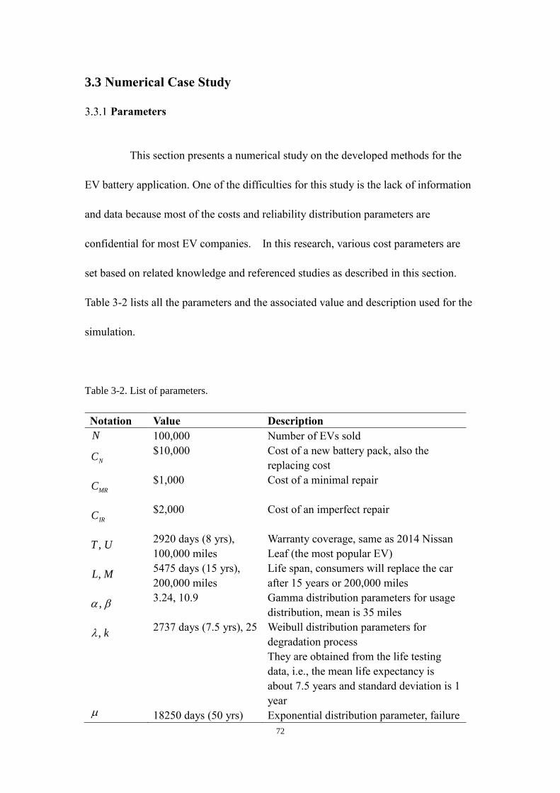
72
3.3 Numerical Case Study
Parameters
This section presents a numerical study on the developed methods for the
EV battery application. One of the difficulties for this study is the lack of information
and data because most of the costs and reliability distribution parameters are
confidential for most EV companies. In this research, various cost parameters are
set based on related knowledge and referenced studies as described in this section.
Table 3-2 lists all the parameters and the associated value and description used for the
simulation.
Table 3-2. List of parameters.
Notation Value Description
100,000 Number of EVs sold
$10,000 Cost of a new battery pack, also the
replacing cost
$1,000 Cost of a minimal repair
$2,000 Cost of an imperfect repair
2920 days (8 yrs),
100,000 miles
Warranty coverage, same as 2014 Nissan
Leaf (the most popular EV)
5475 days (15 yrs),
200,000 miles
Life span, consumers will replace the car
after 15 years or 200,000 miles
3.24, 10.9 Gamma distribution parameters for usage
distribution, mean is 35 miles
2737 days (7.5 yrs), 25 Weibull distribution parameters for
degradation process
They are obtained from the life testing
data, i.e., the mean life expectancy is
about 7.5 years and standard deviation is 1
year 18250 days (50 yrs) Exponential distribution parameter, failure
N
NC
MRC
IRC
, T U
, L M
,
, k

73
rate is
0, 18250 days (50 yrs) The lower and upper limits of the uniform
distribution
The parameters of the Bass diffusion
model for sales prediction
Results
The cost results are summarized in Table 3-3. A manufacturer pays every
repair/replacement during the warranty period and customers pay any fees beyond the
warranty. It is reasonable to assume that each battery pack may have no failure, fail
once or up to twice during its warranty period or after the warranty period. As it can
be seen, most of the costs are paid by customers.
Table 3-3. Simulation results
Percentage of the time (%)
No failure Once Twice
No. of replacements paid by manufacturer 60.07 39.93 0
No. of min. repairs paid by manufacturer 86.73 12.44 0.83
No. of imp. repairs paid by manufacturer 86.66 12.31 1.03
No. of replacements paid by customers 33.99 65.39 0.62
No. of min. repairs paid by customers 87.77 11.43 0.80
No. of imp. repairs paid by customers 85.17 14.14 0.69
Costs Mean ($) Min ($) Max ($)
, single unit lifecycle cost for customer 17,104 10,000 23,000
, single unit lifecycle cost for
manufacturer
4,421 0 16,000
, aggregate cost for manufacturer $442.1 Million
1/
, a b
, , , m n p q1, 365
0.08, 2
m n
p q
SCC
SMC
AMC
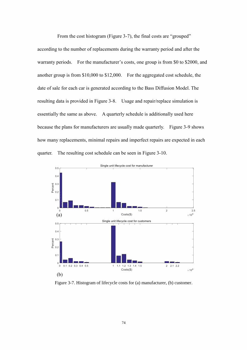
74
From the cost histogram (Figure 3-7), the final costs are “grouped”
according to the number of replacements during the warranty period and after the
warranty periods. For the manufacturer’s costs, one group is from $0 to $2000, and
another group is from $10,000 to $12,000. For the aggregated cost schedule, the
date of sale for each car is generated according to the Bass Diffusion Model. The
resulting data is provided in Figure 3-8. Usage and repair/replace simulation is
essentially the same as above. A quarterly schedule is additionally used here
because the plans for manufacturers are usually made quarterly. Figure 3-9 shows
how many replacements, minimal repairs and imperfect repairs are expected in each
quarter. The resulting cost schedule can be seen in Figure 3-10.
Figure 3-7. Histogram of lifecycle costs for (a) manufacturer, (b) customer.
(a)
(b)

75
Figure 3-8. Probability density function of predicted sales using Bass diffusion model.
0 500 1000 1500 2000 25000
0.005
0.01
0.015
0.02
0.025
0.03
(%)
days
Purchase time distribution (Bass Diffusion)

76
Figure 3-9. Failure schedule for manufacturer for replacements, minimal repairs and
imperfect repairs.
0 2 4 6 8 10 12 140
500
1000
1500
2000
2500
3000Number of replacements per quarter
Years
Num
ber
of
repla
cem
ents
0 2 4 6 8 10 12 140
100
200
300
400
500
600Number of minimal repairs per quarter
Years
Num
ber
of
repairs
0 2 4 6 8 10 12 140
100
200
300
400
500
600Number of imperfect repairs per quarter
Years
Num
ber
of
repairs
77
Figure 3-10. Cost Schedule for manufacturer.
Effects of Altering Battery Reliability and Warranty Period
In the automotive industry, warranty is usually treated as a marketing tool.
For customers, longer warranty periods usually signal better quality or the willingness
to improve the product. Many EV companies also utilize this marketing tool to
increase their sales. For instance, Tesla increased the battery warranty for Model S
three times from 2011 to 2014. It can also be seen in marketing and business
literature. However, the quality assurance aspect of warranty is rarely seen in
engineering literature. For this research, it is also assumed that changing of warranty
terms has no effect on consumer purchasing behavior.
Due to the computational intensive nature of the simulation, the sample size
or the number of customers is assumed to be 10,000 for each case study. The final
0 2 4 6 8 10 12 140
5
10
15
20
25
30Cost Schedule
Years
Mill
ions (
$)
78
total cost is then increased 10 times to simulate 100,000 customers. It is also
assumed that the proportion between time dimension of the warranty and usage
dimension is constant. That is, it is always assumed 1,000 miles per month or
12,000 miles per year, which is the industry standard. For example, a ten-year
warranty also has a 120,000-mile limitation, and a five-year warranty only has a
60,000-mile limitation. This, the percentage of drivers who will reach the time
warranty limit or mileage limit will be the same throughout this section.
Furthermore, the distribution of usage rate is the same. Only the baseline reliability
function will change; the number of batteries above or below the baseline will remain
the same. It is also assumed that the lifecycle is 15 years or 180,000 miles.
Figure 3-11 shows on average how much customers need to pay during the
entire battery lifecycle when the warranty limit and reliability function are varied.
Similarly, Figure 3-12 shows how much the manufacturer needs to pay, and Figure
3-13 shows the total money that the customer and manufacturer combined need to
pay. Note that the total cost is independent of warranty because it only depends on
the number of failures.
From a customer’s perspective, there is a huge incentive to choose a battery
with long warranty. If the true reliability is unknown to them, they may pay more
than $30,000 when the warranty limit is short, and approximately $10,000 (the initial
battery cost, no repair/replace cost) when the warranty limit is long. On the other
hand, the manufacturer is more likely to choose a warranty limit as similar as the
mean breakdown time to minimize the cost it needs to pay. This creates conflict
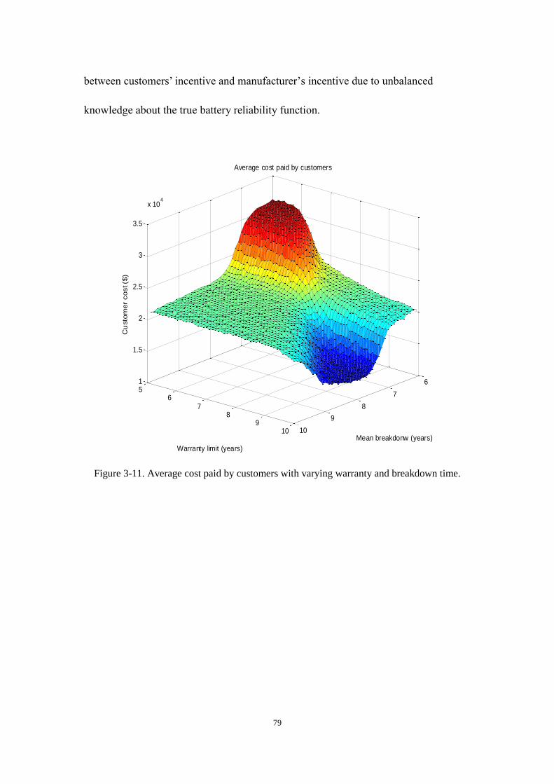
79
between customers’ incentive and manufacturer’s incentive due to unbalanced
knowledge about the true battery reliability function.
Figure 3-11. Average cost paid by customers with varying warranty and breakdown time.
6
7
8
9
10
56
78
910
1
1.5
2
2.5
3
3.5
x 104
Mean breakdonw (years)
Average cost paid by customers
Warranty limit (years)
Cu
sto
mer
cost ($
)

80
Figure 3-12. Average cost paid by manufacturer with varying warranty and breakdown time.
6
7
8
9
10
5
6
7
8
9
10
0
2000
4000
6000
8000
10000
12000
Mean breakdonw (years)
Average cost paid by manufacturer
Warranty limit (years)
Cu
stom
er
cost (
$)

81
Figure 3-13. Average total cost when warranty and reliability functions are varied.
For the aggregated cost schedule, , Figure 3-14 shows when
keeping reliability function the same and only changes warranty limit. When
warranty limit is shorter than the mean breakdown time, most batteries don’t break
during the warranty period. This is due to the standard deviation for the base
reliability function is set around 1. When warranty limit is longer than the mean
breakdown time, the cost schedule is about the same. This is also due to relatively
small standard deviation for the reliability function and also the “grouping” effect
seen in Figure 3-7. During this time, most failures are covered by the manufacturer,
not by customers. Figure 3-15 shows the cost schedule is very sensitive to warranty
change. Even 0.2-year increments in warranty limit can result in a drastic change in
67
89
104
6
8
10
2
2.2
2.4
2.6
2.8
3
3.2
x 104
Warranty limit (years)
Average total cost
Mean breakdonw (years)
Cu
stom
er
cost (
$)
( )AMC t

82
the cost schedule (y-axis).
Figure 3-14. Cost schedule when reliability remains constant and warranty changes.
0 2 4 6 8 10 12 140
0.5
1Cost Schedule, warranty limit = 7 years, mean breakdown = 8 years
Years
Mill
ions (
$)
0 2 4 6 8 10 12 140
5
10Cost Schedule, warranty limit = 8 years, mean breakdown = 8 years
Years
Mill
ions (
$)
0 2 4 6 8 10 12 140
20
40Cost Schedule, warranty limit = 9 years, mean breakdown = 8 years
Years
Mill
ions (
$)
0 2 4 6 8 10 12 140
20
40Cost Schedule, warranty limit = 10 years, mean breakdown = 8 years
Years
Mill
ions (
$)

83
Figure 3-15. Cost Schedule, constant reliability function, and warranty limit change in small
increments.
Keeping warranty limit constant and changing reliability function also has
the similar effect. The plots are shown in Figure 3-16. It also can be seen that the
replacement cost is predominant in both Figure 3-14 and Figure 3-16. In fact, more
than 90% of the costs are incurred by battery replacement.
0 2 4 6 8 10 12 1405
10Cost Schedule, warranty limit = 7.8 years, mean breakdown = 8 years
Years
Mill
ions (
$)
0 2 4 6 8 10 12 1405
10Cost Schedule, warranty limit = 8.0 years, mean breakdown = 8 years
Years
Mill
ions (
$)
0 2 4 6 8 10 12 140
1020
Cost Schedule, warranty limit = 8.2 years, mean breakdown = 8 years
Years
Mill
ions (
$)
0 2 4 6 8 10 12 140
2040
Cost Schedule, warranty limit = 8.4 years, mean breakdown = 8 years
Years
Mill
ions (
$)
0 2 4 6 8 10 12 140
2040
Cost Schedule, warranty limit = 8.6 years, mean breakdown = 8 years
Years
Mill
ions (
$)

84
Figure 3-16. Cost schedule when warranty is constant, altering reliability function.
Effects of Altering Costs
When the IR, MR and replacement costs are changed, there is no effect on
the number of repairs/replaces. However, it can be viewed as putting different
weights on different types of repairs/replaces. That is, they can change the
significance of different types of repairs. Although it is not popular in literature,
when a component fails within an automotive system, it is more likely to be replaced
rather than repaired when in the earlier period of warranty. Thus, it is an important
decision factor when design warranty and battery reliability. However, due to the
setup of the simulation, predominant costs are from battery replacement. Changing
costs in minimal repair and imperfect repairs essentially have only limited effect on
0 2 4 6 8 10 12 140
50Cost Schedule, warranty limit = 8 years, mean breakdown = 7 years
Years
Mill
ions (
$)
0 2 4 6 8 10 12 140
5
10Cost Schedule, warranty limit = 8 years, mean breakdown = 8 years
Years
Mill
ions (
$)
0 2 4 6 8 10 12 140
0.5
1Cost Schedule, warranty limit = 8 years, mean breakdown = 9 years
Years
Mill
ions (
$)

85
both and , and additionally the aggregated cost schedule.
Effects of Purchasing Time Function (Sales Prediction)
To understand how the prediction of sales as an input to the model affect the
life cycle costs, the results based on the Bass fusion function can be compared with
two alternative distributions: uniform distribution and an arbitrary triangle
distribution. As shown in Figure 3-17, it turns out that altering purchase time
function has virtually no effect on different cost types. This is due to the fact that
when combining sales distribution with breakdown function, it is essentially taking
the convolution of these two functions. Any high frequency information such as the
shape of the distribution is lost after the convolution (Liang, Jin, & Ni, 2014).
Because of this, a less-accurate prediction of sales may still result in an accurate
prediction of cost schedule as long as the total number of customers and how many
years it plans to sell are correct. Note that for all three sales distributions, the
majority of the batteries are bought within 3 years.
SCC SMC

86
Figure 3-17. Changing in Sales distribution results virtually no change in costs.
3.4 Conclusions
This chapter investigates the methods for estimating lifecycle warranty cost
for EV batteries with a two-dimensional warranty model. This research attempts to
shift the traditional view of warranty from a simple production protection and
marketing tool to a more intimate link between customers and manufacturers. This
also builds a foundation for future automotive business model development. Effects of
altering influence factors, such as life expectancy (reliability), sales, and return
behavior, are also studied. For battery reliability, an AFT model is used to extrapolate
the base reliability function to drivers with different usage rates. Three types of
0 500 1000 1500 2000 25000
0.02
0.04
pd
f (%
)
days
Purchase time: Bass Diffusion Function
0 500 1000 15000
0.005
0.01
0.015
pd
f (%
)
days
Purchase time: Uniform Distribution
0 500 1000 15000
0.01
0.02
0.03
pd
f (%
)
days
Purchase time: Triangular Distribution
0 5 100
20
40Cost Schedule, Bass Diffusion
Years
Mill
ions (
$)
0 5 100
10
20
30Cost Schedule, Uniform
Years
Mill
ions (
$)
0 5 100
20
40Cost Schedule, Triangular
Years
Mill
ions (
$)

87
failures are modeled to cover various failure modes of EV batteries – Replacement for
entire pack, minimal repair and imperfect repair. Simulation models are developed to
estimate the warranty-related aggregated costs for customers and manufacturers
respectively. From a numerical study on the effects of various influencing factors, it is
found that customers, who have limited knowledge about the true battery life, have
greater incentives to choose battery with long warranty because they try to minimize
the risks of paying repair costs after warranty expires. However, EV manufacturers
prefer to select a warranty limit similar to the mean breakdown time. Therefore,
there exists a tradeoff between the customer’s incentive and manufacturer’s incentives
for the optimal decision on warranty limit. The methods for warranty cost estimation
provide a useful tool for manufacturers to design their warranty scheme, and the
results additionally provide some guidelines for the directions of technology
improvement to further reduce the warranty costs to both sides.

88
CHAPTER 4
CHAPTER 4
Remanufacturing Supply and Demand Matching For EV Battery
Packs
4.1 Introduction
The first EV introduced to the United States, the Honda Insight, appeared in
1999. Even with numerous governmental incentives for consumers to purchase an EV
since then, the market share of EV cars is currently only about 1% of the total car
sales in the US. One major factor is that both the initial cost and the life-cycle cost
of an EV are significantly higher than that of normal internal combustion engine
(ICE) vehicles. Battery packs are the main contributor for this high cost. It is
estimated that it costs Tesla $195 per kWh and GM $215 kWh to produce their battery
packs in 2016 (InsideEVs, 2016). Moreover, the product lifecycle cost, or the cost to
own an EV during its entire life is also dramatically higher compared to ICE vehicles.
This is due to the shorter lifespan of the battery packs compared to that of the vehicle
itself. Battery packs in current generation EVs can only last 5 to 7 years under the
engineering specifications for vehicle power batteries. However, the average
ownership of passenger vehicles is around 12 years. This means a battery pack

89
needs to be replaced during the lifetime of a car.
Currently, this is not an issue because the majority of the EV batteries have
not reached their end-of-life. In addition, to attract more customers, EV
manufacturers (OEMs) usually provide a liberal warranty, even at a loss. In many
cases, battery warranty period is sufficiency long such that if the old battery degrades,
a replacement battery is provided by the OEM at the OEM’s expense.. At present,
because of marketing reasons and generous investors’ support, this is implementable.
However, this is not sustainable and cannot be a long-term strategy simply because
many EV OEMs are operating at loss.
Furthermore, battery technology cannot keep up with the industry. Even
though some manufacturers, such as Tesla, claim that battery cell’s price can go to
$100 per kWh by 2025 (GreenTechMedia, 2016), the battery pack for a Tesla Model S
will still cost more than $15,000 to produce, if other related electronics are included.
On the other hand, a brand-new low trim Honda Civic, a very popular small size
sedan, only costs $16,000. So, OEMs are desperately trying to lower the battery cost
and cannot entirely reply on technology improvements.
One way to solve this problem is to remanufacture the battery packs. It is
estimated that remanufacturing an EV battery costs 20% of the original cost (Jin et al.,
2013), and remanufactured batteries can be used as battery replacement after the first
battery retires. The intuition is very straightforward: if battery warranty is eight
years and the battery fails during the seventh year, the manufacturer only needs to
replace a battery that last for one year or longer. A new battery that can last seven or

90
eight years is excessive. Moreover, if a battery dies during the ninth year and the
customer only wants to use the car for 12 years, this customer can buy a battery
replacement that can last for three years. He/she most likely does not want to spend
another $15,000 ~ $20,000 for a new battery replacement.
To implement this business model successfully, a better understanding of
the interaction between the customer and OEMs during the entire car lifecycle is
required. The goal of this chapter is to demonstrate a way to characterize the
relationship between the customer and OEM, and to determine the feasibility of a
remanufacturing business model. Additionally, an optimal solution is determined for
the model.
This chapter is organized as the following: Section 4.2 gives an overview of
EV battery pack remanufacturing operation. Section 4.3 illustrates what factors can
influence remanufacturing supply side and how they are influenced. Similarly,
Section 4.4 demonstrates demand side behavior. In Section 4.5, different demand-
supply matching mechanisms are evaluated, and an optimal solution is provided at the
end. Conclusion and future direction is stated in the final conclusion section.
4.2 Remanufacturing
Remanufacturing may have different meanings in different industries. In
this research, it is the process to reconstruct a product to certain specifications from
field returned used products and/or newly manufactured components. One aspect
that is different from other industries is that the final remanufactured product may

91
contain newly produced components.
Although remanufacturing has been studied and implemented for decades,
one of its fundamental challenges, namely matching supply side and demand side
fluctuations and uncertainties, is still largely untouched. For traditional
manufacturing, only demand side (customer side) has large fluctuations. Through
different supply chain regulations, supply side fluctuations can be viewed as
controllable and predictable. On the other hand, remanufacturing supply relies on
customer returns, and it is highly uncontrollable and unpredictable. This is one of the
main reasons why remanufacturing only flourishes in a handful of industries, where
both demand and supply are highly predictable or “buffers” can easily be placed.
Here, buffers can take many forms, such as the high profit margin in medical devices,
aerospace or large machinery industries. Because profit margin is high, it is still
profitable after a 30% to 40% fluctuation. Other buffers, such as inventory, are also
commonly used. Besides buffers, other mechanisms, such as contracts, are often
used to regulate supply-demand uncertainties. For example, many printer OEMs
sign contracts with their large customers and guarantee the cartridge and toner usage
for certain period. During this time period, the return and supply of cartridge and
toner replacements can be regulated by the printer OEMs. Essentially, it creates a
“closed loop” between OEMs and customers.
The key of this research is to reduce both the demand side and supply side
fluctuations and uncertainty by creating a similar “closed loop” between EV OEMs
and customers. To establish this loop, the traditional one-time contact relationship

92
(car purchasing) needs to be extended to a lifelong relationship. Luckily, modern EV
OEMs, such as Tesla, also operate their own repair centers and charge stations (gas
station equivalent), and car warranties can be used similar to the printer
cartridge/toner contracts. By implementing more effective warranty and
repair/remanufacturing policies, OEMs can better forecast customers’ behavior and
have a more predictable and controllable remanufacturing system.
For this research, discrete event simulation (DES) is used to model different
scenarios. DES models systems as a sequence of events and/or states. Each one of
them occurs at a particular time and is affected by other events and/or states. Here,
events can be human actions, such as EV purchasing, deciding which battery module
to remanufacture, or a mechanical module, such as degradation and break down of
battery packs. Pure analytical model is not implemented due to the complicated
interconnections between events.
4.3 Supply Side
Overview
Supply side is where customers supply used battery packs so
remanufacturers can transform them into remanufactured ones. For this research,
only failed and returned batteries are considered. Certain end-of-Life (EOL)
scenarios, such as batteries from discarded cars due to their old-age or replaced by
newly purchased cars, are not considered because they are difficult for
remanufacturers to collect. That is, the main source of returned batteries comes from
93
repair centers. It is also assumed that those repair centers and remanufacturing
centers are operated by EV OEMs, thereby enabling OEMs to coordinate their
inventories and actions. For example,, Tesla owns all its repairing centers and
remanufacturing centers. Since Tesla did not open its diagnosis tools and internal
protocols to public, it is very difficult or impossible for third party repair shops to
diagnose and repair Tesla’s battery packs. It is also true for the Nissan Leaf, Chevy
Volt and most other EV models. One reason is that the detailed battery control
scheme is still a closely guarded trade secret and EV makers’ competitive advantage.
Compared to the supply side of traditional manufacturing, remanufacturing
supply varies greatly in the returned parts’ quality, quantity and return time. One of
the aims of this chapter is to characterize this variation, learn its effects, and
determine ways to reduce its effects.
Supply Variation Influential Factors
Some influential factors are borrowed directly from previous chapters. Sales
estimation is represented by the same Bass Diffusion model from Chapter 2 and 3.
Usage rate is also the same Gamma distribution from previous chapter. For
warranty, the standard two dimensional non-renewing free replace/repair warranty
with effective warranty and scaled by the usage rate is also the same as previous
chapter. New influential factors are added as the following.
94
4.3.2.1 Vehicle End-of-Use Date
Vehicle end-of-use date is considered because during simulation, sometimes
the expected end-of-use date takes place before first battery break down or warranty
expiration. According to CNBC (CNBC, 2015), the average length of a car life in the
United States is currently around 12 years. Some cars can be used as high as 20 years,
and some others only used for 5 to 6 years. For simplicity, a truncated normal
distribution is used to simulate expected car life. Truncated normal distribution has
many normal distribution properties, yet it has a finite support.
2
( )( )
( ( ) ( ) )
wher e
1 1( ) exp( ) , and
22
1( ) (1 ( ) )
2 2
t
pdf tb a
er f
.
(4-1)
Here, the mean of the distribution is months or 12 years, standard
deviation months or 2 years. It is truncated at months and
months or 20 years. The shape of the distribution is illustrated in Figure
4-1
144
24 6a
240b

95
Figure 4-1. Car life distribution.
4.3.2.2 Battery Reliability, Degradation Process and Failures
For this research, four types of failures are considered: electronic
components, frame/enclosure, battery cell physical and battery cell degradation
failures. Like many complex systems, Li-ion battery packs are built into a
hierarchical structure. The pack is made of a number of battery modules
interconnected by an electronic power/communication network and controlled by a
battery management system (BMS). Each module, in turn, consists of a number of
battery cells interconnected by a module level network and controlled by a module
controller. For this research, the remanufacturing process in consideration

96
disassembles modules from an old pack and remanufactures it into a new pack. The
disassembly on battery cell level is not considered here.
For electronic components failures, BMSs, module controllers, electronic
power/communication network at different levels, and different sensors (voltage,
current, temperature, vibration sensors at different levels) failures are included.
Frame/enclosure failures usually are comprised of punctures and breakages of
different kind, different leakages, and other physical damages to the battery frame or
enclosure. Battery cell physical failures include physical damages at the cell level,
such as broken connections, internal shorts, and internal opens. These failures are
often caused by driving conditions, such as physical vibration, extreme temperature
change, metal fatigue and so on. For these three types of failures, when a component
has truly failed, it is discarded. There is no remanufacturing or reuse of this
component anymore, because it is cheaper to replace a new one than to remanufacture
an old one. Finally, battery cells can age and degrade, thereby producing a gradual
decrease in capacity. Failure status is reached when a battery degrades to certain
threshold, such as 70% of its original capacity.
For this research, electronic components are all grouped together and their
failures are represented by a Weibull distribution. All physical module failures are
grouped together and represented by another Weibull distribution. Similarly,
frame/enclosure failures are also modeled according to Weibull distribution. Weibull
distribution is commonly used for both electronics and mechanical failures (Rinne,
2008). The reason these three failure types are separated and not grouped as one is

97
because their diagnosis processes are different and treated differently during repair
that will be explained in detail in the repair type section. A Weibull distribution has
the form of:
1( ) exp( ( ) ) , 0( )
0,
k kk tt t
pdf t
ot her wi se
, (4-2)
where is the shape parameter and is the scale parameter or the so
called “failure rate” of the Weibull distribution.
For the simulation, it is assumed that there are 10 modules in a battery pack.
If one fails, the entire pack needs to be repaired. Likewise, any component fails, it is
sent to a repair center for diagnosis. For electronics, the shape parameter is
assumed to be 5, and . For frame/enclosure,
and . For module physical failures, and
. Thus, all the electronics related components have
failure rate of one per 30 years or 360 months, and mechanical parts have failure rate
of one per 25 years or 300 months. The shape parameter k determines the standard
deviation or how the distribution will spread. Moreover, because there are 10
modules, all 10 module failures are simulated and the pack failure depends on the first
module failure. If the rest of modules are used in remanufactured packs, their
distribution will not be reset. That is, from simulation’s perspective, a module’s
physical failure date is set when the module object is created in simulation. The
0k 0
k
1 / (30 12) 1 / 360 4k
1 / ( 25 12) 1 / 300 4k
1 / (30 12) 1 / 360

98
distributions are shown in Figure 4-2
Figure 4-2. Distributions for pack electronics, frame/enclosure and module physical failures.
4.3.2.3 Battery Degradation Process and Related Failures
GM wrote in its newest 2016 Chevy Bolt’s Manual on page 322 that
“Depending on use, the battery may degrade as little as 10% to as much as 40% of
capacity over the warranty period.” (Trek, 2016) Its warranty period is standard 8

99
years or 100,000 miles. For other EV OEMs, such as Tesla, degradation is excluded
from their warranty completely. From the “fine print” of its warranty on its official
website, Tesla states:
“The Battery, like all lithium-ion batteries, will experience gradual
energy or power loss with time and use. Loss of Battery energy or
power over time or due to or resulting from Battery usage, is NOT
covered under this Battery Limited Warranty.”
Both quotes clearly illustrate that battery capacity degradation is a serious
issue in EV industry.
The Li-ion battery aging mechanism has been studied extensively in the
past decade. Many efforts have been devoted to physics-based model including
electrochemical model, equivalent circuit model, etc. However, data driven methods
such as reliability function or statistical failure behavior are generally unknown
because it requires a large number of run-to-fail battery test data. Unfortunately, most
of the degradation data for commercial EV battery packs are confidential to EV
OEMs. Reliability functions generally are inference from either known degradation
processes or real measured condition metrics, such as crack size, loss of efficiency
and other factors. In this research, the degradation processes of the Li-ion battery
can be modeled using existing techniques, such as first hitting threshold time (FHTT),
to transfer the physics-of-failures (PoF) to reliability functions (Letot & Dehombreux,

100
2009; Lee & Whitmore, 2006; Van Noortwijk et al., 2005). Once a base reliability
function is developed for average drivers with an average usage rate, an Accelerated
Failure Time (AFT) model is used to extrapolate the base reliability function to
drivers with different usage rates. It is also assumed that the degradation process is
only influenced by time and usage. Other causes, such as operating temperature,
state of charge for each cycle, charge protocols, and driving patterns, are not
considered in this research.
If is a random variable representing failure time, the reliability function
and its complementary, failure functions, are the same as equations (3-10) to (3-13).
Different parameters of these equations are obtained using equations (3-8) and (3-9).
As discussed in Chapter 3, reliability function can be affected by usage rate.
Accelerated Failure Time model is used to scale reliability function in the time
domain. The scaling process and the parameters used are the same as equations
(3-14) to (3-16).
4.3.2.4 Combine Failure Types
After a customer purchases an EV, the first failure is the first occurrence of
the combination of all four failure types. Subsequent failures are more difficult to
determine analytically because it depends on how the first failure is repaired and if a
remanufactured battery pack is used as replacement. The distribution of the first
failure is shown in Figure 4-3. Notice that almost half of the failures will take place

101
before the warranty expiration date (eight years or 96 months). However, after
taking effective warranty into account, the number of failures is much smaller (not
shown in graph) because both the warranty and degradation process need to take
usage rate into account. Even with considering this factor, a change in failure type
composition can be seen in Table 4-1, which is generated by the DES simulation.
Figure 4-3. First failure date.
Table 4-1. Simulated failure type composition before and after warranty period.
Failure types % before warranty expiring % after
Electronics 18 24
Frame/enclosure 15 27
Module physical related 20 22
Module degradation related 47 27
102
Remaining Useful Life (RUL)
Remaining Useful Life (RUL) of a module is the key parameter to
determine if a module still can be used for remanufacturing. There are several
methods to express the RUL of a battery, such as remaining capacity. For a more
consistent comparison, and simpler calculation, estimated remaining useable time is
used for this research. For example, if a battery module is simulated to last for 10
years or 120 months, and the usage rate is 40 miles/day, the module failure date due to
degradation is changed to: 120 months / 40 miles/day * 35 mils/day = 105 months.
If the battery pack is returned due to electronics failure at year eight or 96th month, the
RUL is (105 months – 96 months) * 40 miles/day / 35 miles/day = 10.3 months.
RUL needs to be scaled back, so different modules can compare with each other.
Supply During Market Lifetime
Market lifetime is defined from the time the first product is sold to the time
the last product is discarded by its user. A sample run is illustrated in Figure 4-4,
and the simplest remanufacturing condition is used for this plot. Namely, all
replaced batteries are remanufactured, and inventory is infinite. Battery modules are
also used based on the principle of closest capacity to match. The conditions will be
explained in detail in the matching section. In Figure 4-4, the date axis displays
when a remanufacturable module is returned to the remanufacturing center, and the
RUL axis shows the quality. The return date ranges from around the second year

103
(24th month) all the way to 16th year (200th month), and RUL ranges from one month
to about 10 years (120 months). Return date is much longer than the lifespan of a
battery, mainly because the car purchase date is added. It is also due to the usage
rate scaling. It is evident that return date peaks when return date is 90 months and
RUL is 70 months. The electronics, frame/enclosure failures are the main
contributor for the peak. This is different from Table 4-1 because subsequent
failures and remanufactured battery pack failure are also considered here. Table 4-1
only considers the first failure for new battery packs.

104
Figure 4-4. Supply during market life (3D view and top view).
Major Assumptions for the Supply Side
There are several major assumptions for the supply side. Namely,
All the distributions are independent from each other. All the interactions
between them are not considered, such as earlier product may have lower
reliability than later product.
No second-hand ownership is considered. That is, no warranty, usage rate
or degradation changes.
Usage rate is constant, and no events outside the four types of failures are
considered, such as accidents.

105
Battery degradation rate is constant for each module throughout the life-
time of the module unless it is remanufactured into another battery pack.
The degrading rates are different for different modules in the same pack.
Assume a linear degradation, and failures follow Weibull distribution.
100% diagnosis accuracy. All the failures can be diagnosed exactly, and
degradation rate is also known.
100% repairing/remanufacturing rate. There is no repair or
remanufacturing loss.
No transportation, diagnosis or repairing/remanufacturing time. Because
the time unit for this research is month, and the transportation and
remanufacturing time usually are one or two weeks which is much less than
the time scale here. This also implies that there is no geographic barrier, all
the inventory around the world can act as one.
Failures are 100% detectable by customer. When customers see a warning
indicator on dashboard, they send their car to repair center without
delaying.
No third-party involved. EV companies, such as Tesla, do not sell spare
parts and diagnosis tools to third party and do not provide specs for the
diagnosis codes.
4.4 Demand Side

106
Overview
Unlike traditional demand, remanufacturing demand is defined by four
factors: time, price, quantity and quality (RUL). It characterizes how many of a
remanufactured product is wanted by customer at each time interval, each price level
and each quality level. Because there is only one supplier of the remanufactured
batteries, price is fixed. Hence, only the other three factors are considered.
Two Types of Demands
Two types of demands are separated into the time dimension by warranty
expiration date. Before this date, demand is from the OEM/remanufacturer because
the product is paid by the OEM directly. The OEM additionally decides the quality
of the product. To minimize the cost of battery replacement, the lowest suitable
quality remanufactured battery is supplied to the customer. For this research, a half-
year “safeguard” is added. For example, if warranty is eight years, and the battery
pack is failed at year six with usage rate of 40 miles/day, a RUL of (2 year + 0.5
year)/35 miles/day * 40 miles/day = 2.86 years remanufactured pack is supplied.
For the simulation, the cost is additionally added to the OEM.
After the warranty, customers decide the demand. Two types of battery
can be chosen from: brand new and remanufactured. Here, the RUL for
remanufactured units is calculated as the difference between expected car end-of-use
date and return time plus a safeguard of half year, and usage rate is also applied as

107
before. For the simulation, it is assumed that 80% of customers will purchase a
remanufactured battery, 20% new, chosen at random. The cost is added to customer.
Failure Types and Demanded Parts
As stated in Section 4.3.2.2, there are four types of failures. Each type of
failure will demand different type of parts and the reliability function will be set or
reset differently. Generally speaking, when a battery pack is sent to a repair center,
both failure and module degradation condition is checked. If a failure is found, the
related part will be replaced. At the same time, if a module cannot last until the end
of the warranty period, it is also replaced. It is repair center’s goal to ensure no more
failure or degradation will take place before warranty ends. After warranty period,
because it is not EV OEM’s responsibility to ensure the condition of the battery, repair
centers only check for failures. The repairing/replacement policy for simulation is
summarized in Table 4-2.
Table 4-2. Parts replacement and remanufacturing policy.
Warranty
Expiration
Failure Types Failed Part Modules
Before Electronics Replace with new,
reset part reliability
function to new
Check if other modules can last
till warranty expiration. If not,
replace with remanufactured
having right RUL. If cannot
find, use higher RUL; still
cannot find, use new parts. Set
reliability function according to
condition.
Frame/enclosure Replace with new, Check if other modules can last

108
reset part reliability
function to new
till warranty expiration. If not,
replace with remanufactured
with right RUL. If cannot find,
use higher RUL; still cannot
find, use new parts. Set
reliability function according to
condition.
Module
physical
Replace with
remanufactured, set
reliability function
according to
condition
Check if other modules can last
till warranty expiration. If not,
replace with remanufactured
with right RUL. If cannot find,
use higher RUL; still cannot
find, use new parts. Set
reliability function according to
condition.
Module
degraded
Replace with
remanufactured, set
reliability function
according to
condition
Check if other modules can last
till warranty expiration. If not,
replace with remanufactured
with right RUL. If cannot find,
use higher RUL; still cannot
find, use new parts. Set
reliability function according to
condition.
After Electronics Replace with new,
reset part reliability
function to new, or
replace entire pack
new
Do nothing
Frame/enclosure Replace with new,
reset part reliability
function to new, or
replace entire pack
new
Do nothing
Module
physical
Replace part with
remanufactured, or
replace entire pack
new
Do nothing
Module
degraded
Replace part with
remanufactured, or
replace entire pack
new
If not replaced with new pack,
check other modules can last as
long. If not, customer pay to
replace

109
Demand during Market Lifetime
Unlike the supply side, which is determined mainly by the natural
degradation process and failures, demand during market lifetime is mainly determined
by how a battery is diagnosed, repaired and replaced, and other human factors. It
can be seen from Figure 4-5 that the demand peaks when return date is approximately
95 months and RUL is 14 months. Note that the RUL axis starts from the sixth
month. This is because six months of safeguard is added for all remanufactured
packs, as stated in section 4.4.2.

110
Figure 4-5. Demand during market lifetime (3D and top view). Both Return Date and RUL
are in months.
Major Assumptions for the Demand Side
There are a number of assumptions for the demand side:
Consumers behave rationally and their behavior is predictable. For
example, they will retire their EV only if the expected end-of-life time is
reached.
Consumer behavior will not be changed by outside factors. For example,
if an EV fails 3 or 4 times, they still keep it and drive it as before.
No geographic consideration is included. Customers from all over the world
will behave the same.

111
Repair center knows all about drivers, such as usage rate (total driven
distance divided by time).
Inventory cost is neglected.
4.5 Demand and Supply Matching
Overview
The goal of the matching process is to shift both supply and demand (Figure
4-4 and Figure 4-5) simultaneously such that the overlap between them can be
maximized. A number of “shifting enablers” are considered. However, each one of
them can only change certain aspects of supply or demand curves. By combining
them together, the best optimization may be achieved.
For this research, the total cost for manufacturer is used as the objective
function in the optimization. The following cost assumptions are additionally made:
For a new battery pack, electronics costs $500 and frame and enclosure cost $1000,
and a single module costs $2000. Thus, a brand-new pack costs $21,500 in total.
For repairing and remanufacturing, transportation fee from repairing center to
remanufacturing center is $200 per pack, diagnosis fee is $200, repairing is $100, and
remanufacturing is $100 per module. Labor costs are included in these fees. For
inventory, the cost is $5/module/month. It is assumed that there is no inventory cost
for other non-module or non-pack items. For a simple scenario, a battery pack fails
before the warranty expiration date. After diagnosis, a battery management system

112
(BMS) is replaced, and 2 modules are also replaced by remanufactured ones because
they cannot last till warranty expiration date. The BMS is replaced at repairing
center and 2 modules are replaced at remanufacturing center since modules are stored
at remanufacturing centers. The total cost is $200 diagnosis cost + $200
transportation cost + $100 repairing cost + $500 new electronics (BMS) cost + $100 x
2 module remanufacturing cost = $1200 + inventory cost for the 2 modules.
Repairing/Remanufacturing Policies
Four repairing policies are considered for analysis. The first is to replace
all failed parts with new packs. This was performed on some EV models during
their early dates since no repairing or remanufacturing facility was built, and it was
more economical to provide a new pack than spend manpower to diagnose and repair.
The second policy is to replace all failed components with new components. The
third one is to replace failed modules with remanufactured modules. The detail of
this policy is stated in Table 4-2. The fourth policy is to use remanufactured
replacement according to current inventory. For example, if a module with RUL of
1.5 years is demanded, but most common RUL in inventory is three years at this
moment, then module that has RUL of three years is used. However, if demand RUL
is greater than most common RUL inventory, demand RUL is used. The purpose for
the fourth policy is to lower the inventory cost, and to extend battery life by supplying
better modules.
The result is shown in Table 4-3. Four columns of the table correspond to

113
the four repairing and remanufacturing policies. The first 11 rows show the break
down by event sequences. The letters are coded as: B = breakdown, W = end of the
warranty, and C = end of car life. For example, CW means there is no failure, and
end of car life happens before warranty ends, and BBWBC means a battery breaks
twice before warranty and breaks once between warranty ends and end of the car life.
This helps both debugging the DES simulation during development and having an
overall picture of when and why batteries may fail after the simulation is done.
Percent supply used is the total percentage of supply being used during the entire
market time. It can be seen that without optimization only around half of supply is
used. Similarly, demand is also not entirely met. OEM average cost is mainly the
cost OEMs spend on warranty. Average customer cost is the cost after the warranty.
The sum of these two are the total cost needed for the entire lifecycle. OEM total
cost is the total cost OEM needs to spend on all of the batteries during the entire
market life. It can be shown in Table 4-3 that, although no matching/optimization is
done, the costs for both customer and OEM are decreased significantly. This decrease
is due to the cost of remanufactured parts being significantly lower than brand new
parts.
Table 4-3. Failure and cost break down during market life by remanufacturing policy types.
New
pack
New
Part
Reman.,
RUL
Reman.,
inventory
CW (count) 5009 4966 5015 5020
BCW (count) 10046 9041 7032 8067
BBCW (count) 5092 5924 8018 7021
WC (count) 9951 9012 9011 8958

114
BWC (count) 30922 11001 11903 13071
BBWC (count) 6981 17933 15060 12992
BBWBC (count) 1041 6029 8958 7938
BWBC (count) 8057 10091 10021 9003
BWBBC (count) 947 7096 7988 7096
WBC (count) 20962 11045 7955 11097
WBBC (count) 1018 7915 8954 9985
Percent supply used (%) 0 0 47.90% 56.45%
Percent demand satisfied (%) 0 0 58.24% 64.29%
OEM average cost ($) 15783.39 8954.42 6129.25 5858.77
Customer average cost ($) 9137.90 9689.26 6724.87 6645.39
OEM + cust. average cost ($) 24921.29 18643.68 12854.12 12504.16
OEM total cost ($B) 1.58 0.90 0.61 0.59
Warranty Policies
Changing warranty policies is always a complicated marketing decision
because it may potentially change the market share significantly. Therefore, the
traditional terms, such as time and miles driven are not changed here. A new
dimension, charging cycle, is added. As stated in the warranty section, the battery
failure due to degradation currently is not included in warranty for many EV makers.
Here, charging cycles only affect capacity degradation, and the hope is that the market
behavior will not be altered.
It is concluded that Li-ion battery degradation depends on its charging and
discharging cycles (Zhang, 2006). Charging/discharging cycle dependent warranty
currently exists in many industries where Li-ion batteries are used. It is very
common in electric power tools and machineries. Milwaukee tools’ warranty
guarantees 5 years or 2000 charging cycles (Tools, 2016). It is also common in
consumer electronics, such as HP laptops and Apple computers. Golf carts, such as
115
EzGo, also offer similar warranties.
There are several ways to calculate the charging cycles. Apple laptops,
such as MacBook and MacBook Pro use simple sum of all charging. For example,
today it is charged 30%, from 70% to 100%, and tomorrow it is charged 80%, from
10% to 90%. The sum of them is 110% or 1.1 charging cycle. Because
charging/discharging profile can affect degradation profoundly, some other companies
use weighted sum that may favor shorter charging periods or in favor of certain
percentage range. For simplicity, the straightforward sum is used for this research.
Similar to usage rate, charging rate or charging cycle per month is
used here. It is a random variable that will also stay constant over the entire vehicle
lifecycle. It is different from usage rate because of drivers’ driving behavior
differences. Usage rate only depends on how far a car is driven, and charging rate is
also influenced by driving profile, such as accelerations and average speed. As
shown in equation (4-3), a scaling factor is created to scale the usage rate.
When , average driving profile is assumed. When , it
represents a more aggressive driver. When , it characterizes a less
aggressive driver. The charging cycle limit is also first transferred to the warranty
time dimension to generate the effective time, then compared with other two warranty
dimensions to create effective warranty, as shown in equation (4-3).
(4-3)
( )Ct
( )Dt
( ) 1Dt ( ) 1Dt
0 ( ) 1Dt
l i m
l i m
( ) ( ) ( )C
Ct Rt DtU

116
(4-4)
For the DES simulation, is assumed to be an inverse normal
distribution with mean at , and shape factor , so is normally
distributed. It is also assumed that the car can drive 200 miles/charge cycle on
average. The distributions are shown in Figure 4-6.
Figure 4-6. Distribution of driving profile scaler, D (top) and charging cycle per month, C
(bottom).
The effect of changing the total number of charging cycles for warranty on
both remanufacturing supply and demand curves is shown in Figure 4-7. It is
evident that both supply and demand curves only shifted upward slightly in “return
mi n( , / , / )end ef f ef f
EW T U r C c
( )Dt
1 20 1( )Dt

117
date” direction. This shift is mainly due to the fact that the charging cycles per
month are highly dependent on usage rate, and effective warranty is also dependent on
the other two warranty dimensions. However, as charging cycle limit increases, both
supply and demand curves are shifted to low “RUL” direction. This shift is due to
the increasing likelihood of module degradation failures. Intuitively, if more
charging cycles are allowed (relative to driving distance and usage time), more
aggressive driving (higher acceleration, higher speed) will more likely be included.
For these more aggressive drivers, module degradation failures are more likely to
occur.
Figure 4-7. Effects of changing total warranty charging cycles on supply and demand. Both
RUL and Date are in months.
Inventory Policies
Unlike other types of policies, inventory policy only changes supply curve.

118
This gives managers the freedom to plan the demand curve first, then adjust supply
accordingly. Essentially, by changing different inventory policies, supply curve can
be shifted in the “return date” direction. That is, the new supply time can be viewed
as the sum of original supply time and storage time. Ideally, if the managers can
obtain a perfect prediction of demand at different RUL levels, they can shift supply
accordingly to have a perfect fit. However, because demand cannot be predicted
flawlessly, different inventory policies need to be tested, and are discussed in this
section. Here, the inventory is assumed to be first-in-first-out (FIFO).
Three types of inventory policies are considered.
To store everything as in previous sections.
To divide RUL levels into categories, and set different quantity limitations
(inventory cap) on different categories. If a limit is reached, new supply
of this category will be discarded.
To divide RUL levels into categories again, and set different time
limitations on different categories. If a module is stored pass the time
limitation, it is discarded.
For this section, all simulation parameters are the same as in section 4.4.3,
and only inventory parameters are different. It is assumed RUL only ranges from
zero to 150 months. Either 5 categories (30 months per category) or 10 categories
(15 months per category) are tested. The limitations are optimized using genetic
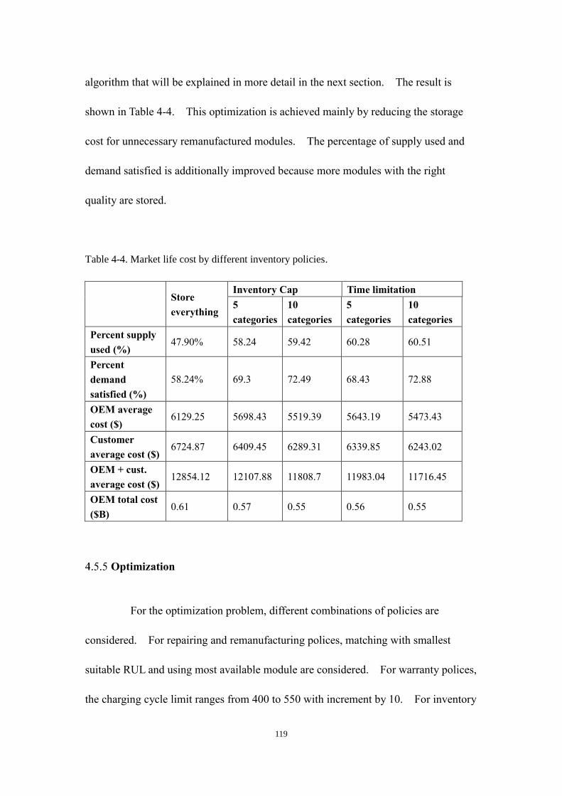
119
algorithm that will be explained in more detail in the next section. The result is
shown in Table 4-4. This optimization is achieved mainly by reducing the storage
cost for unnecessary remanufactured modules. The percentage of supply used and
demand satisfied is additionally improved because more modules with the right
quality are stored.
Table 4-4. Market life cost by different inventory policies.
Store
everything
Inventory Cap Time limitation
5
categories
10
categories
5
categories
10
categories
Percent supply
used (%) 47.90% 58.24 59.42 60.28 60.51
Percent
demand
satisfied (%)
58.24% 69.3 72.49 68.43 72.88
OEM average
cost ($) 6129.25 5698.43 5519.39 5643.19 5473.43
Customer
average cost ($) 6724.87 6409.45 6289.31 6339.85 6243.02
OEM + cust.
average cost ($) 12854.12 12107.88 11808.7 11983.04 11716.45
OEM total cost
($B) 0.61 0.57 0.55 0.56 0.55
Optimization
For the optimization problem, different combinations of policies are
considered. For repairing and remanufacturing polices, matching with smallest
suitable RUL and using most available module are considered. For warranty polices,
the charging cycle limit ranges from 400 to 550 with increment by 10. For inventory

120
policies, inventory limitations and time limitations are considered, and both 5-
category and 10-category types are tested. Two objective functions are used. One
is the total OEM cost during the entire market life, and the other is the sum of both
OEM and all customers’ costs during the entire market life. One is from
manufacturer/remanufacturer’s perspective, and the other is from society’s
perspective. Standard non-negative constraints are used.
A global mixed integer optimization algorithm, genetic algorithm, is used
because the optimization problem may be non-linear and non-differentiable in nature,
and several variables are discrete. Because of DES simulation programming
complexity, two repairing/remanufacturing policies are ran separately and the results
are combined to obtain the final solution. It is illustrated in Table 4-5 that the
charging cycle limit is the binding factor (limited by the charging cycle range
restrictions) for OEM cost minimization. However, if warranty terms are set too
strictly, customers and media will doubt the quality and reliability of the product.
On the other hand, OEM plus customer cost minimization seems to take another
extreme on the spectrum. The result additionally shows that the inventory capacity
limitation is in favor for both minimization objectives. Other observation is that the
average OEM plus customers’ costs are very similar for both objectives. This
similarity may be caused by the rapid increasing in lower RUL portion and rapid
decreasing in higher RUL portion in for both supply and demand curves. Thus,
when overlapping them, “boundaries” are significant.

121
Table 4-5. Optimization results.
Objective function OEM OEM + customer
Percent supply used (%) 62.42 62.84
Percent demand satisfied (%) 74.39 74.45
OEM average cost ($) 5215.87 5245.59
Customer average cost ($) 6084.59 5858.94
OEM + cust. average cost 11300.46 11104.53
repair/reman policy RUL RUL
Charging cycle limit 400 530
Limitation Inv. Cap Inv. Cap
Category 1 103,697 111,292
Category 2 118,864 147,617
Category 3 130,016 135,059
Category 4 139,153 144,303
Category 5 37,645 72,041
Category 6 70,840 45,442
Category 7 40,833 31,113
Category 8 13,096 11,259
Category 9 980 2,292
Category 10 2,262 1,393
Major Assumptions for Matching
There are also a number of assumptions associated with the matching process.
No degradation during storage. It is reported batteries degrades even
when they are sitting on the shelf. However, it is small comparing to the
degradation while driving.
Only one generation of batteries. This means modules are exchangeable.
No geographical consideration. Essentially, it is assumed all the batteries
are stored and remanufactured in one place and perfect information sharing
between repairing centers, so they know if there is a remanufactured

122
module with right RUL for them to use.
4.6 Conclusion
An EV battery pack remanufacturing discrete event system simulation study
is performed in order to explore the feasibility of lowering the total market lifetime
cost for both EV OEM and customers via remanufacturing automotive components.
Several influential factors are considered, such as warranty, different battery failure
modes and driving behavior. Key factors are also used for optimization, such as
repairing and remanufacturing strategies and inventory policies. Although there are
a number of aspects of the remanufacturing process that are not included in this study
(many of them are listed in the assumption sub-sections at the end of supply, demand
and matching segments), this study provides a good understanding of how a
remanufacturing process may behave in real-life settings.

123
CHAPTER 5
CHAPTER 5
Conclusion and Future Work
5.1 Conclusion and Contributions
This dissertation focuses on creating the “loop” between a remanufacturing
system, customer and a manufacturing system. The major achievements of this
dissertation can be summarized as follows.
In Chapter 2, the “quarter loop” is created. Namely, the loop between
manufacturer and customer is formed. The remanufacturing supply side is studied.
Instead of treating core return as completely random, a more regulated scheme
through warranty is considered. Instead of using disaggregated approach, such as
time series, a new aggregated approach of remanufacturing supply forecast is
provided. An analytical model is stated and verified by discrete event simulations.
In Chapter 3, the “half loop” is created. Again, the “loop” links
manufacturer and customers. Unlike Chapter 2, both the remanufacturing supply and
demand sides are considered here. The four types of costs for the warranty are
illustrated: single item cost to OEM, single item cost to customer, aggregated cost to
OEM and cost schedule for OEM. All the influential factors in Chapter 2 are
124
considered. In addition, warranty and battery degradation processes and failure
processes are considered.
In Chapter 4, the “full loop” is created. All three parties; the manufacturer,
customer and remanufacturer are included. Different supply-demand matching
approaches are considered, such as a new warranty dimension policy, different repair
and remanufacturing polices and different inventory policies. An optimization
model using the above policies is provided.
Comparing with other remanufacturing researches, this study expands the
existing remanufacturing system to including customers and manufacturing system,
and a holistic approach is provided. The academic contributions of this research can
be summarized as follows.
Unlike traditional manufacturing, remanufacturing processes need to make
a closed loop approach between customers and manufacturers/remanufacturers. The
traditional view of “supply-side” and “demand-side” does not necessarily apply
because customers can be both “demand-side” of products and “supply-side” of
returned cores. Similarly, a manufacturer/remanufacturer can also be both the
“demand-side” and “supply-side.” The border between these two parties can be
blurry depending on one’s view point. It becomes natural to include both sides into
one system. This research, rather than treating customers’ behavior as
uncontrollable events like many other remanufacturing research, it aims at influencing
customers through warranty and other contracts.
Furthermore, this dissertation considers both quality and quantity attributes
125
for both demand and supple of remanufactured goods. Unlike traditional
manufacturing, the essence of remanufacturing is to turn the returned core of various
quality levels to a better or higher quality level finished goods. Thus, when
characterizing both the demand and supply for remanufacturing, quality is a critical
attribute. Yet, it is not considered thoroughly in preceding research. In addition,
the relationship between return date and the quality of return cores is also studied.
This provides a more realistic and useful estimation for the supply side.
Once quality and quantity variations are considered, it is natural to provide
a matching mechanism to ensure the right quality and quantity from both supply-side
and demand-side are met. Chapter 4 provides a number of such matching
mechanisms, such as different inventory storage policies, repairing policies, and
warranty types. Chapter 4 also shows that matching mechanisms are essentially
used to shift various categories of returned cores along the quality axis and return date
axis of the three-dimensional demand and supply curves. By employing different
matching mechanisms, the cost of remanufacturing can be dramatically lowered.
Traditionally, variations in production systems are dealt with buffers. Buffers may
be storage, capacity, time, profit, investment and many other types of manufacturing
related characteristics. Essentially, buffering is to add additional capability or
abilities to filter out the fluctuations. Storage, or inventory, is used to shift past
production capacity (already produced parts) to an instance in the future.
Investments and loans are shifting future virtual capacity (money from future sold
products) to the past. Capacity buffer is to install additional devices in parallel.

126
Time buffer is to increase the order wait time or back order size. Similar to
opportunity cost, time buffer essentially uses the wait time as opportunity capacity.
From using “passive” buffers, this research explores the possibility of using different
“active” matching mechanisms to cope with variations, and provides additional means
to reduce the effects of those variations.
Diverse types of costs are also considered, such as single item cost to
manufacturer, single item cost to customer, aggregated cost to manufacturer,
aggregated cost schedule. Hence, a more holistic picture is provided for
manufacturers, customers and regulators. Because of the cost schedule, quarterly,
monthly, and weekly remanufacturing plans can be established.
A novel genetic based matching algorithm was additionally developed to
minimize the total cost for manufacturers. This algorithm is capable of mixed
categories and employs variable optimization which is suitable for the matching
process.
5.2 Proposed Future Work
Chapter 4 listed a number of assumptions for all supply side, demand side
and matching mechanisms. Relaxing any of them can be a new research direction.
Major future work directions can be:
1. Different battery generations can be considered. Some generations can be only
backward compatible, while other generations can provide both forward and
backward compatibility.

127
2. Include geographic considerations. Currently, the entire world is treated as a
single zone. It is unrealistic to ship battery packs from Asia to North America or
to Europe. Different zones can be considered.
3. Second hand EVs can be studied. Many factors can be different, such as
warranty, usage rate, degradation, trading between ownerships and so on. This
will affect the dynamics of both the supply and demand sides.
4. Realistic failure and degradation processes can be considered. Weibull
distribution is used for almost all failure and degradation processes. This simple
approach may not capture everything realistically.

128
BIBLIOGRAPHY
DriveClean. (2016). Plug-in Electric Vehicle Resource Center: Define your incentives
search. Retrieved from
https://driveclean.arb.ca.gov/pev/Incentives.php?submit=submit&bev=1
EVVolumes. (2016). The Electric vehicle world sales database. Retrieved from
http://www.ev-volumes.com/datacenter/us/monthly-ev-sales
GreenTechMedia. (2016). How Soon Can Tesla Get Battery Cell Costs Below $100
per Kilowatt-Hour. Retrieved from
https://www.greentechmedia.com/articles/read/How-Soon-Can-Tesla-Get-
Battery-Cell-Cost-Below-100-per-Kilowatt-Hour/
InsideEVs. (2016). Monthly Plug-In Sales Scorecard. Retrieved from
http://insideevs.com/monthly-plug-in-sales-scorecard/
Tools, M. (2016). Charge Limited Warranty. Retrieved from
https://www.milwaukeetool.com/press-releases/five-year2000-charge-limited-
warranty-for-all-v-technology-lithium-ion-batteries
Trek, E. (2016). GM Chevy Bolt EV Battery Degradation. Retrieved from
https://electrek.co/2016/12/07/gm-chevy-bolt-ev-battery-degradation-up-to-
40-warranty/
Autoblog.com. (2015). Six-week production shutdown planned for 2016 Chevy Volt.
Retrieved from http://hotair.com/archives/2012/08/27/gm-to-shut-down-
chevy-volt-plant-for-four-weeks-for-the-second-time-this-year/
CNBC. (2015). Americans holding onto their cars longer than ever. Retrieved from
http://www.cnbc.com/2015/07/28/americans-holding-onto-their-cars-longer-
than-ever.html
Hirsch, J. (2015). Elon Musk's growing empire is fueled by $4.9 billion in
government subsidies. LA Times.
InsideEVs. (2015). Monthly Plug-in Sales Scorecard. Retrieved from
http://insideevs.com/monthly-plug-in-sales-scorecard/

129
Radio, M. (2015). GM Extends Summer Shutdown at Volt Factory. Retrieved from
http://michiganradio.org/post/gm-extends-summer-shutdown-volt-factory
George, P. (2014). Fiat Loses $14,000 Every Time Someone Buys Their Electric Car.
Retrieved from http://jalopnik.com/sergio-marchionne-doesnt-want-you-to-
buy-a-fiat-500e-1579578914
GM. (2014). GM Invests $449 Million for Next Generation Electrification.
Retrieved from
http://media.gm.com/media/us/en/gm/news.detail.html/content/Pages/news/us/
en/2014/Apr/0408-investment.html
Liang, X., Jin, X., & Ni, J. (2014). Forecasting product returns for remanufacturing
systems. Journal of Remanufacturing, 4(1), 8.
Samaras, P. (2014). Fiat Loses $14,000 Every Time Someone Buys Their Electric Car.
Retrieved from http://jalopnik.com/sergio-marchionne-doesnt-want-you-to-
buy-a-fiat-500e-1579578914
Shahan, Z. (2014). Electric Vehicle Market Share in 19 Countries. Retrieved from
http://www.abb-conversations.com/2014/03/electric-vehicle-market-share-in-
19-countries
Bigman, D. (2013). Driverless Cars Coming To Showrooms By 2020, Says Nissan
CEO Carlos Ghosn. Forbes. Retrieved from
http://www.forbes.com/sites/danbigman/2013/01/14/driverless-cars-coming-
to-showrooms-by-2020-says-nissan-ceo-carlos-ghosn/
Jin, X., Hu, S. J., Ni, J., & Xiao, G. (2013). Assembly strategies for remanufacturing
systems with variable quality returns. IEEE Transactions on Automation
Science and Engineering, 10(1), 76-85.
Smart, J., Powell, W., & Schey, S. (2013). Extended Range Electric Vehicle Driving
and Charging Behavior Observed Early in the EV Project (0148-7191).
Retrieved from
Urken, R. (2013). Tesla Debacle Highlights Need for New EV Battery Technology.
Retrieved from
http://www.forbes.com/sites/rosskennethurken/2013/02/12/tesla-debacle-
highlights-need-for-new-ev-battery-technology/
Bigman, D. (2012). Driverless Cars Coming to Showrooms by 2020, Says Nissan
CEO Carlos Ghosn. Retrieved from
http://www.forbes.com/sites/danbigman/2013/01/14/driverless-cars-coming-

130
to-showrooms-by-2020-says-nissan-ceo-carlos-ghosn
Clottey, T., Benton, W., & Srivastava, R. (2012). Forecasting product returns for
remanufacturing operations. Decision Sciences, 43(4), 589-614.
Hensley, R., Newman, J., Rogers, M., & Shahinian, M. (2012). Battery technology
charges ahead. McKinsey Quarterly, 3, 5-50.
Jin, X. (2012). Modeling and analysis of remanufacturing systems with stochastic
return and quality variation. General Motors Company.
King, D. (2012). Lithium-ion Battery Costs Will Still Be About $400/kWh by 2020.
Retrieved from http://green.autoblog.com/2012/04/06/lithium-ion-battery-
costs-will-still-be-about-400-kwh-by-2020/
Price, B., Dietz, E., & Richardson, J. (2012). Life cycle costs of electric and hybrid
electric vehicle batteries and end-of-life uses. Paper presented at the
Electro/Information Technology (EIT), 2012 IEEE International Conference
on, 1-7.
Pundit, A. (2012). GM to Shut down Chevy Volt plant for Four Weeks –for the
Second Time This Year,” HotAir.com. Retrieved from
http://hotair.com/archives/2012/08/27/gm-to-shut-down-chevy-volt-plant-for-
four-weeks-for-the-second-time-this-year/
Ramsey, M. (2012). Ford CEO: Battery is Third of Electric Car Cost. Retrieved
from
http://online.wsj.com/news/articles/SB10001424052702304432704577350052
534072994?mg=reno64-
wsj&url=http%3A%2F%2Fonline.wsj.com%2Farticle%2FSB1000142405270
2304432704577350052534072994.html
Smith, K., Earleywine, M., Wood, E., Neubauer, J., & Pesaran, A. (2012).
Comparison of plug-in hybrid electric vehicle battery life across geographies
and drive cycles (0148-7191). Retrieved from
Varnosafaderani, S., & Chukova, S. (2012). An imperfect repair strategy for two-
dimensional warranty. Journal of the Operational Research Society, 63(6),
846-859.
AutoWeek. (2011). Chrysler will lose $10,000 on every Fiat 500 EV it sells, CEO
Says. Retrieved from http://autoweek.com/article/green-cars/chrysler-will-
lose-10000-every-fiat-500-ev-it-sells-ceo-says

131
Blischke, W. R., Karim, M. R., & Murthy, D. P. (2011a). Cost models for two-
dimensional warranties Warranty Data Collection and Analysis (pp. 137-157):
Springer.
Blischke, W. R., Karim, M. R., & Murthy, D. P. (2011b). Warranty data collection and
analysis: Springer Science & Business Media.
Dubarry, M., Liaw, B. Y., Chen, M.-S., Chyan, S.-S., Han, K.-C., Sie, W.-T., & Wu,
S.-H. (2011). Identifying battery aging mechanisms in large format Li ion
cells. Journal of Power Sources, 196(7), 3420-3425.
Ghoreishi, N., Jakiela, M. J., & Nekouzadeh, A. (2011). A cost model for optimizing
the take back phase of used product recovery. Journal of Remanufacturing,
1(1), 1.
Jin, X., Ni, J., & Koren, Y. (2011). Optimal control of reassembly with variable
quality returns in a product remanufacturing system. CIRP Annals-
Manufacturing Technology, 60(1), 25-28.
Pearre, N. S., Kempton, W., Guensler, R. L., & Elango, V. V. (2011). Electric vehicles:
How much range is required for a day’s driving? Transportation Research
Part C: Emerging Technologies, 19(6), 1171-1184.
Voelcker, J. (2011). One million plug-in cars by 2015?[Update]. IEEE Spectrum,
48(4).
Wong, Y., Lu, W.-F., & Wang, Z. (2011). Life cycle cost analysis of different vehicle
technologies in Singapore.
Loveday, E. (2010, 5/15/2010). WSJ: Nissan Leaf profitable by year three; battery
cost closer to $18,000. AutoBlog. Retrieved from
http://green.autoblog.com/2010/05/15/nissan-leaf-profitable-by-year-three-
battery-cost-closer-to-18/
Loveday, E. (2010). WSJ: Nissan Leaf Profitable by Year Three; Battery Cost Closer
to $18,000. Retrieved from http://green.autoblog.com/2010/05/15/nissan-
leaf-profitable-by-year-three-battery-cost-closer-to-18/
Letot, C., & Dehombreux, P. (2009). Degradation models for reliability estimation
and mean residual lifetime. Paper presented at the Proceedings of the 8th
National Congress on Theoretical and Applied Mechanics, 618-625.
Baik, J., & Murthy, D. P. (2008). Reliability assessment based on two-dimensional
warranty data and an accelerated failure time model. International Journal of

132
Reliability and Safety, 2(3), 190-208.
Rinne, H. (2008). The Weibull distribution: a handbook: CRC Press.
Samaras, C., & Meisterling, K. (2008). Life cycle assessment of greenhouse gas
emissions from plug-in hybrid vehicles: implications for policy: American
Chemical Society.
Sutherland, J. W., Adler, D. P., Haapala, K. R., & Kumar, V. (2008). A comparison of
manufacturing and remanufacturing energy intensities with application to
diesel engine production. CIRP Annals-Manufacturing Technology, 57(1), 5-8.
Hanafi, J., Kara, S., & Kaebernick, H. (2007). Generating fuzzy coloured petri net
forecasting model to predict the return of products. Paper presented at the
Electronics & the Environment, Proceedings of the 2007 IEEE International
Symposium on, 245-250.
Majeske, K. D. (2007). A non-homogeneous Poisson process predictive model for
automobile warranty claims. Reliability Engineering & System Safety, 92(2),
243-251.
Chukova, S., & Johnston, M. (2006). Two-dimensional warranty repair strategy based
on minimal and complete repairs. Mathematical and computer modelling,
44(11), 1133-1143.
Lee, M.-L. T., & Whitmore, G. (2006). Threshold regression for survival analysis:
modeling event times by a stochastic process reaching a boundary. Statistical
Science, 501-513.
Murthy, D. P., & Blischke, W. R. (2006). Warranty management and product
manufacture: Springer Science & Business Media.
Sahay, B., Srivastava, S. K., & Srivastava, R. K. (2006). Managing product returns for
reverse logistics. International Journal of Physical Distribution & Logistics
Management, 36(7), 524-546.
Zhang, S. S. (2006). The effect of the charging protocol on the cycle life of a Li-ion
battery. Journal of Power Sources, 161(2), 1385-1391.
Van Noortwijk, J., Kallen, M., & Pandey, M. (2005). Gamma processes for time-
dependent reliability of structures. Advances in safety and reliability,
proceedings of ESREL, 1457-1464.
Baik, J., Murthy, D., & Jack, N. (2004). Two‐dimensional failure modeling with

133
minimal repair. Naval Research Logistics (NRL), 51(3), 345-362.
Lilien, G. L., & Rangaswamy, A. (2004). Marketing engineering: computer-assisted
marketing analysis and planning: DecisionPro.
Sarre, G., Blanchard, P., & Broussely, M. (2004). Aging of lithium-ion batteries.
Journal of Power Sources, 127(1), 65-71.
Ting Lee, M. L., Whitmore, G., Laden, F., Hart, J. E., & Garshick, E. (2004).
Assessing lung cancer risk in railroad workers using a first hitting time
regression model. Environmetrics, 15(5), 501-512.
Toktay, L. B., van der Laan, E. A., & de Brito, M. P. (2004). Managing product
returns: the role of forecasting Reverse Logistics (pp. 45-64): Springer.
Buxcey, I. (2003). Remanufacturing in the Automotive Industry. In A. P. R.
Association (Ed.).
Guide, V. D. R., & Wassenhove, L. N. (2003). Business aspects of closed-loop supply
chains (Vol. 2): Carnegie Mellon University Press Pittsburgh, PA.
Hauser, W., & Lund, R. T. (2003). The remanufacturing industry: anatomy of a giant.
Boston University, Boston.
Iskandar, B. P., & Blischke, W. R. (2003). Reliability and warranty analysis of a
motorcycle based on claims data. Case Studies in Reliability and Maintenance,
623-656.
Oliva, R., & Kallenberg, R. (2003). Managing the transition from products to
services. International journal of service industry management, 14(2), 160-
172.
Jeong, K. S., & Oh, B. S. (2002). Fuel economy and life-cycle cost analysis of a fuel
cell hybrid vehicle. Journal of Power Sources, 105(1), 58-65.
Marx-Gomez, J., Rautenstrauch, C., Nürnberger, A., & Kruse, R. (2002). Neuro-fuzzy
approach to forecast returns of scrapped products to recycling and
remanufacturing. Knowledge-Based Systems, 15(1), 119-128.
Yang, G., & Zaghati, Z. (2002). Two-dimensional reliability modeling from warranty
data. Paper presented at the Reliability and Maintainability Symposium, 2002.
Proceedings. Annual, 272-278.
Broussely, M., Herreyre, S., Biensan, P., Kasztejna, P., Nechev, K., & Staniewicz, R.

134
(2001). Aging mechanism in Li ion cells and calendar life predictions. Journal
of Power Sources, 97, 13-21.
Delucchi, M. A., & Lipman, T. E. (2001). An analysis of the retail and lifecycle cost
of battery-powered electric vehicles. Transportation Research Part D:
Transport and Environment, 6(6), 371-404.
Westkämper, E., Alting, L., & Arndt, G. (2001). Life cycle management and
assessment: approaches and visions towards sustainable manufacturing.
Proceedings of the Institution of Mechanical Engineers, Part B: Journal of
Engineering Manufacture, 215(5), 599-626.
Gaines, L., & Cuenca, R. (2000). Costs of lithium-ion batteries for vehicles; Argonne
National Laboratory. Center for Transportation Research. Argonne, IL.
Guide, V. D. R. (2000). Production planning and control for remanufacturing: industry
practice and research needs. Journal of operations Management, 18(4), 467-
483.
IJESD, A. (2000). Costs of lithium-ion batteries for vehicles. Center for
Transportation Research, Argonne National Laboratory.
Toktay, L. B., Wein, L. M., & Zenios, S. A. (2000). Inventory management of
remanufacturable products. Management science, 46(11), 1412-1426.
Guide, V. D. R., Jayaraman, V., & Srivastava, R. (1999). Production planning and
control for remanufacturing: a state-of-the-art survey. Robotics and Computer-
Integrated Manufacturing, 15(3), 221-230.
Hammond, R., Amezquita, T., & Bras, B. (1998). Issues in the automotive parts
remanufacturing industry: a discussion of results from surveys performed
among remanufacturers. Engineering Design and Automation, 4, 27-46.
Ayres, R., Ferrer, G., & Van Leynseele, T. (1997). Eco-efficiency, asset recovery and
remanufacturing. European Management Journal, 15(5), 557-574.
Smith, S. W. (1997). The scientist and engineer's guide to digital signal processing.
Pham, H., & Wang, H. (1996). Imperfect maintenance. European journal of
operational research, 94(3), 425-438.
Urban, G. L., Weinberg, B. D., & Hauser, J. R. (1996). Premarket forecasting of
really-new products. The Journal of Marketing, 47-60.
135
Lawless, J., Hu, J., & Cao, J. (1995). Methods for the estimation of failure
distributions and rates from automobile warranty data. Lifetime Data Analysis,
1(3), 227-240.
Mahajan, V., Muller, E., & Bass, F. M. (1995). Diffusion of new products: Empirical
generalizations and managerial uses. Marketing Science, 14(3_supplement),
G79-G88.
Nahmias, S., & Cheng, Y. (1993). Production and operations analysis (Vol. 2): Irwin
Homewood, IL.
Kelle, P., & Silver, E. A. (1989). Forecasting the returns of reusable containers.
Journal of operations Management, 8(1), 17-35.
Goh, T., & Varaprasad, N. (1986). A statistical methodology for the analysis of the
life-cycle of reusable containers. IIE transactions, 18(1), 42-47.
Lund, R. T. (1984). Remanufacturing. Technology review, 87(2), 18-19.
Lund, R. T. (1983). Remanufacturing, United States experience and implications for
developing nations: Center for Policy Alternatives, Massachusetts Institute of
Technology.
Sharif, M. N., & Islam, M. N. (1980). The Weibull distribution as a general model for
forecasting technological change. Technological Forecasting and Social
Change, 18(3), 247-256.
Pinder, J. E., Wiener, J. G., & Smith, M. H. (1978). The Weibull distribution: a new
method of summarizing survivorship data. Ecology, 59(1), 175-179.