A GARCH Option Pricing Model with Filtered Historical Simulation∗

Giovanni Barone-Adesi†

Swiss Finance Institute

University of Lugano

Robert F. Engle

Stern School of Business

New York University

Loriano Mancini

Swiss Banking Institute

University of Zurich

Review of Financial Studies, Vol. 21, 2008, 1223–1258

∗For helpful comments, we thank Yacine Aıt-Sahalia (the editor), two anonymous referees, Fulvio Corsi, Robert

Elliott, Jens Jackwerth, and Claudia Ravanelli. Financial support from the NCCR-FinRisk Swiss National Science

Foundation (Barone-Adesi and Mancini) and the University Research Priority Program “Finance and Financial Mar-

kets” University of Zurich (Mancini) is gratefully acknowledged. Addresses for Robert Engle and Loriano Mancini:

Robert Engle, Stern School of Business, New York University, 44 West Fourth Street, New York, NY 10012, USA, E-mail

address: rengle@stern.nyu.edu; Loriano Mancini, Swiss Banking Institute, University of Zurich, Plattenstrasse 32,

CH-8032 Zurich, Switzerland, E-mail address: mancini@isb.uzh.ch.†Corresponding Author: Giovanni Barone-Adesi, Swiss Finance Institute at the University of Lugano, Via Buffi 13,

CH-6900 Lugano, Switzerland, E-mail address: baroneg@lu.unisi.ch.

1

A GARCH Option Pricing Model with Filtered Historical Simulation

Abstract

We propose a new method for pricing options based on GARCH models with filtered his-

torical innovations. In an incomplete market framework, we allow for different distributions of

historical and pricing return dynamics, which enhances the model’s flexibility to fit market option

prices. An extensive empirical analysis based on S&P 500 Index options shows that our model

outperforms other competing GARCH pricing models and ad hoc Black–Scholes models. We show

that the flexible change of measure, the asymmetric GARCH volatility, and the nonparametric

innovation distribution induce the accurate pricing performance of our model. Using a nonpara-

metric approach, we obtain decreasing state price densities per unit probability as suggested by

economic theory and corroborating our GARCH pricing model. Implied volatility smiles appear

to be explained by asymmetric volatility and negative skewness of filtered historical innovations.

Keywords: Option pricing, GARCH model, state price density, Monte Carlo simulation.

JEL Classification: G13.

2

There is a general consensus that asset returns exhibit variances that change through time.

GARCH models are a popular choice to model these changing variances, as is well documented in

financial literature. However, the success of GARCH in modeling historical return variances only

partially extends to option pricing. Duan (1995) and Heston and Nandi (2000) among others assume

normal return innovations and parametric risk premiums in order to derive GARCH-type pricing

models. Their models consider historical and pricing (i.e., risk neutral) return dynamics in a unified

framework. Unfortunately, they also imply that, up to the risk premium, conditional volatilities of

historical and pricing distributions are governed by the same model parameters. Empirical studies,

for instance by Chernov and Ghysels (2000) and Christoffersen and Jacobs (2004), show that this

restriction leads to rather poor pricing and hedging performances. The reason is that changing

volatility in real markets makes the perfect replication argument of Black and Scholes (1973) invalid.

Markets are then incomplete in the sense that perfect replication of contingent claims using only the

underlying asset and a riskless bond is impossible. Consequently, an investor would not necessarily

price the option as if the distribution of its return had a different drift but unchanged volatility. Of

course markets become complete if a sufficient (possibly infinite) number of contingent claims are

available. In this case, a well-defined pricing density exists.1

In the markets we consider, the volatility (and hence the distribution) of historical and pricing

returns is different. This occurs because investors will set state prices to reflect their aggregate pref-

erences. Our model differs from other models in the financial literature because we rely on market

incompleteness to allow for a pricing distribution that is different in shape from the historical distri-

bution. It is possible then to calibrate the pricing process directly on option prices. Although this

may appear to be a purely fitting exercise, involving no constraint beyond the absence of arbitrage,

the stability of the pricing process over time and across maturities imposes substantial parameter

1For instance, Jarrow and Madan (1995) investigate the hedging of systematic jumps in asset returns when additional

assets are introduced into the market.

3

restrictions. Furthermore, economic theory imposes further restrictions on investor preferences for

aggregate wealth in different states, such as decreasing intertemporal marginal rate of substitutions.

Pricing models are economically validated when these restrictions are satisfied.

This paper presents two main contributions: a new GARCH pricing model and the analysis of

aggregate intertemporal marginal rate of substitutions. An in-depth empirical study underlies the

previous contributions. Our GARCH pricing model relies on the Glosten, Jagannathan, and Runkle

(1993) asymmetric volatility model driven by empirical GARCH innovations. The nonparametric

distribution of innovations captures excess skewness, kurtosis, and other nonstandard features of

return data. We undertake an extensive empirical analysis using European options on the S&P 500

Index from 1/2002 to 12/2004. We compare the pricing performances of our approach, the GARCH

pricing models of Heston and Nandi (2000) and Christoffersen, Heston, and Jacobs (2006), and the

benchmark model of Dumas, Fleming, and Whaley (1998). Interestingly, our GARCH pricing model

outperforms all the other pricing methods in almost all model comparisons. We show that the flexible

change of measure, the asymmetric GARCH volatility, and the nonparametric innovation distribution

induce the accurate pricing performance of our model. To economically validate our approach, we

estimate the state price densities per unit probability (or aggregate intertemporal marginal rate of

substitutions) for all the available maturities in our sample. Compared to previous studies, such

as Jackwerth (2000) and Rosenberg and Engle (2002), we undertake a larger empirical analysis.

More importantly, our estimates of the state price densities per unit probability tend to display the

expected level and shape, as predicted by economic theory.

The financial literature on GARCH pricing models is rather extensive and we provide here only

a partial overview. Heston and Nandi (2000) derive an almost closed form pricing formula, assuming

normal return innovations, a linear risk premium, and the same GARCH parameters for historical

and pricing asset returns. In our pricing model, we rely on Monte Carlo simulations and hence

we can relax their assumptions. Duan (1996) calibrates a GARCH model to the FTSE 100 Index

4

options assuming Gaussian innovations and the locally risk neutral valuation relationship (i.e., same

daily conditional variances under historical and pricing measures). Engle and Mustafa (1992) use a

similar method, calibrating a GARCH model to S&P 500 Index options to investigate the persistence

of volatility shocks under historical and pricing distributions. Recent studies on GARCH pricing

models include, for instance, Christoffersen, Heston, and Jacobs (2006) and Christoffersen, Jacobs,

and Wang (2006), where option prices are computed by using the technique in Heston and Nandi

(2000), inverting moment generating functions.

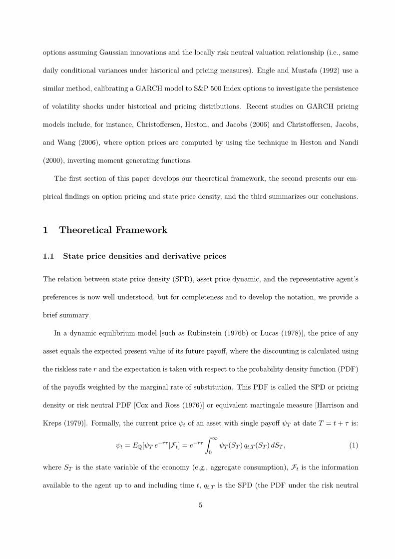
The first section of this paper develops our theoretical framework, the second presents our em-

pirical findings on option pricing and state price density, and the third summarizes our conclusions.

1 Theoretical Framework

1.1 State price densities and derivative prices

The relation between state price density (SPD), asset price dynamic, and the representative agent’s

preferences is now well understood, but for completeness and to develop the notation, we provide a

brief summary.

In a dynamic equilibrium model [such as Rubinstein (1976b) or Lucas (1978)], the price of any

asset equals the expected present value of its future payoff, where the discounting is calculated using

the riskless rate r and the expectation is taken with respect to the probability density function (PDF)

of the payoffs weighted by the marginal rate of substitution. This PDF is called the SPD or pricing

density or risk neutral PDF [Cox and Ross (1976)] or equivalent martingale measure [Harrison and

Kreps (1979)]. Formally, the current price ψt of an asset with single payoff ψT at date T = t+ τ is:

ψt = EQ[ψT e−rτ |Ft] = e−rτ

∫ ∞

0ψT (ST ) qt,T (ST ) dST , (1)

where ST is the state variable of the economy (e.g., aggregate consumption), Ft is the information

available to the agent up to and including time t, qt,T is the SPD (the PDF under the risk neutral

5

measure Q) at time t for payoffs liquidated at date T , and EQ is the expectation under Q. The

security price ψt can be equivalently represented as:

ψt = EP[ψT Mt,T |Ft] =

∫ ∞

0ψT (ST )Mt,T (ST ) pt,T (ST ) dST , (2)

where Mt,T is the SPD per unit probability2 and pt,T is the PDF under the historical or objective

measure P at time t for payoffs liquidated at date T . In a continuum of states, the SPD defines the

Arrow–Debreu [Arrow (1964); and Debreu (1959)] security price. For each state of the economy, s,

qt,T (s) is the forward price of an Arrow–Debreu security paying one dollar at time T if the future

state ST falls between s and s + ds. The SPD per unit probability Mt,T (s) is then the current

market price of an Arrow–Debreu security per unit probability, with an expected rate of return of

1/Mt,T (s) − 1 under the historical measure P. Such expected rates of return depend on the current

state of the economy summarized in the information set Ft.

Equation (2) shows the high information content of the SPD per unit probability. This equa-

tion can be used to determine equilibrium asset prices given historical asset price dynamics and

agent preferences, or to infer agent characteristics given the observed market asset prices. For

instance, in a Lucas (1978) economy, the state variable, ST , is aggregate consumption, CT , and

Mt,T = U ′(CT )/U ′(Ct), which is the intertemporal marginal rate of substitution. Using an uncondi-

tional version of Equation (2) and the aggregate consumption CT as the state variable, Hansen and

Singleton (1982) and Hansen and Singleton (1983) estimate the risk aversion and time preference of

the representative agent, hence identifying the SPD per unit probability. In general the SPD per unit

probability depends on all variables that affect marginal utility, such as past consumption or equity

market returns [see, for instance, the discussion in Rosenberg and Engle (2002, Section 2.1) and ref-

2The SPD per unit probability is also known as the asset pricing kernel [Rosenberg and Engle (2002)] or stochastic

discount factor [see Campbell, Lo, and MacKinlay (1997) and Cochrane (2001) for comprehensive surveys of its role in

asset pricing, and Ross (1978), Harrison and Kreps (1979), Hansen and Richard (1987), and Hansen and Jagannathan

(1991) for related works].

6

erences therein]. Furthermore, due to the well-known measurement problems and the low temporal

frequency of aggregate consumption data,3 several researchers have proposed alternative methods to

estimate Mt,T , substituting consumption data with market data. For instance, Rosenberg and Engle

(2002) project Mt,T onto the payoffs of traded assets ψT , avoiding the issue of specifying the state

variables in the SPD per unit probability. Aıt-Sahalia and Lo (2000) and Jackwerth (2000) adopt

similar approaches, projecting Mt,T onto equity return states using S&P 500 Index option prices.

They assume that investors have a finite horizon and that the equity index level perfectly correlates

with aggregate wealth. In this paper, we also make the same assumptions.4 Our goal is to develop

a pricing model for the derivative securities that takes into account the most important features of

equity returns. The model will be evaluated on the basis of statistical measures (mispricing of ex-

isting securities), as well as economic measures (verifying whether SPD per unit probability satisfies

economic criteria).

1.2 Asset price dynamics

In this section, we develop the stochastic volatility model that captures the most important features

of the equity return process. We use this model for pricing options.

1.2.1 Historical return dynamics. A substantial amount of empirical evidence suggests that

equity return volatility is stochastic and mean reverting, return volatility responds asymmetrically

to positive and negative returns, and return innovations are non-normal [e.g., Ghysels, Harvey,

and Renault (1996)]. In a discrete time setting, the stochastic volatility is often modeled using

extensions of the autoregressive conditional heteroscedasticity (ARCH) model proposed by Engle

3For discussions of these issues see for example Ferson and Harvey (1992), Wilcox (1992), and Slesnick (1998).4See for example Rubinstein (1976a) and Brown and Gibbons (1985) for the conditions under which the SPD per

unit probability with consumption growth rate as state variable is equivalent to a SPD per unit probability with equity

index return as state variable.

7

(1982). Bollerslev, Chou, and Kroner (1992) and Bollerslev, Engle, and Nelson (1994) conducted

comprehensive surveys of the ARCH and related models. In a continuous time setting, the stochastic

volatility diffusion model is commonly used; surveys of this literature are conducted by Ghysels,

Harvey, and Renault (1996) and Shephard (1996).

To model the equity index return, we use an asymmetric GARCH specification with an empirical

innovation density. The GARCH model of Bollerslev (1986) accounts for stochastic, mean reverting

volatility dynamics. The asymmetry term is based on Glosten, Jagannathan, and Runkle (1993)

(GJR) hereafter. The empirical innovation density captures potential non-normalities in the true

innovation density and we refer to this approach as the filtering historical simulation (FHS) method.

Barone-Adesi, Bourgoin, and Giannopoulos (1998) introduce the FHS method to compute portfolio

risk measures and Engle and Gonzalez-Rivera (1991) investigate the theoretical properties of the

GARCH model with empirical innovations.

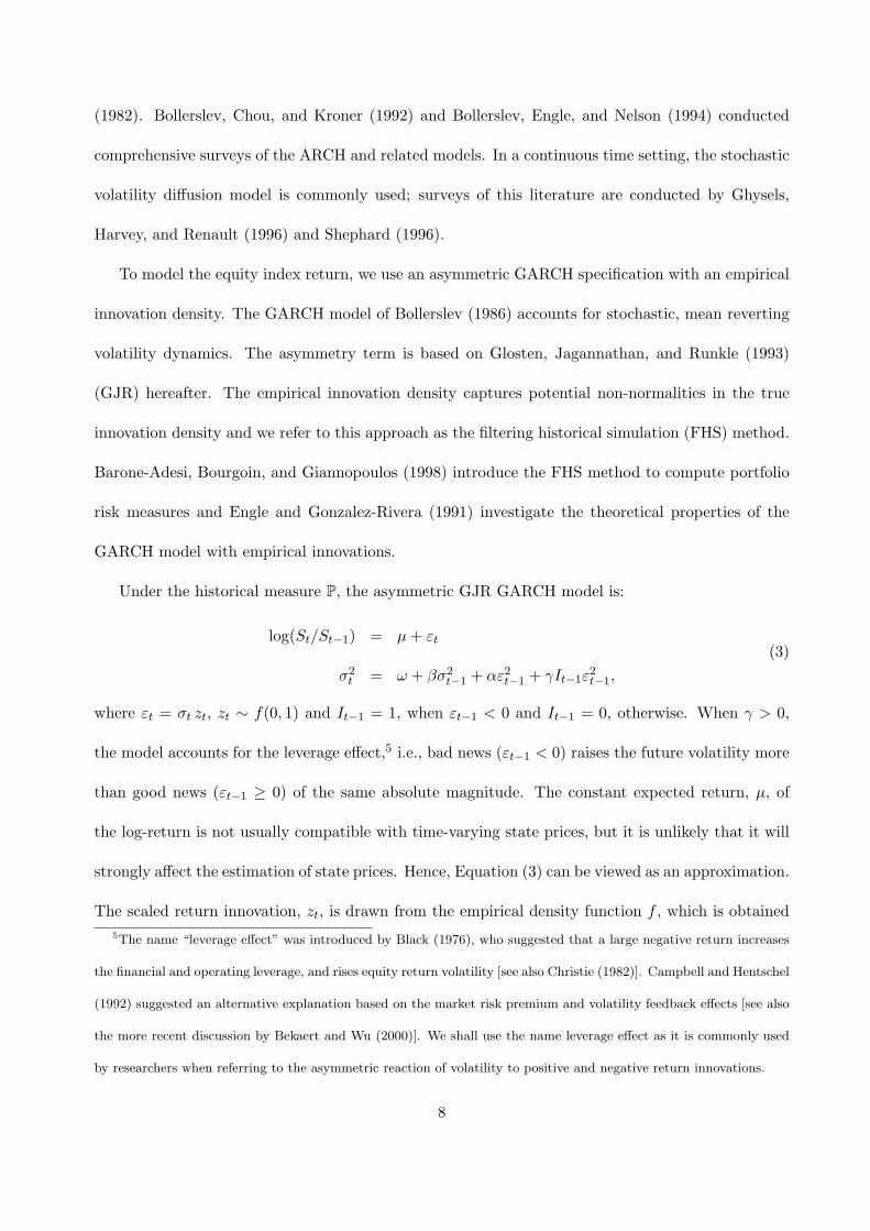
Under the historical measure P, the asymmetric GJR GARCH model is:

log(St/St−1) = µ+ εt

σ2t = ω + βσ2

t−1 + αε2t−1 + γIt−1ε2t−1,

(3)

where εt = σt zt, zt ∼ f(0, 1) and It−1 = 1, when εt−1 < 0 and It−1 = 0, otherwise. When γ > 0,

the model accounts for the leverage effect,5 i.e., bad news (εt−1 < 0) raises the future volatility more

than good news (εt−1 ≥ 0) of the same absolute magnitude. The constant expected return, µ, of

the log-return is not usually compatible with time-varying state prices, but it is unlikely that it will

strongly affect the estimation of state prices. Hence, Equation (3) can be viewed as an approximation.

The scaled return innovation, zt, is drawn from the empirical density function f , which is obtained

5The name “leverage effect” was introduced by Black (1976), who suggested that a large negative return increases

the financial and operating leverage, and rises equity return volatility [see also Christie (1982)]. Campbell and Hentschel

(1992) suggested an alternative explanation based on the market risk premium and volatility feedback effects [see also

the more recent discussion by Bekaert and Wu (2000)]. We shall use the name leverage effect as it is commonly used

by researchers when referring to the asymmetric reaction of volatility to positive and negative return innovations.

8

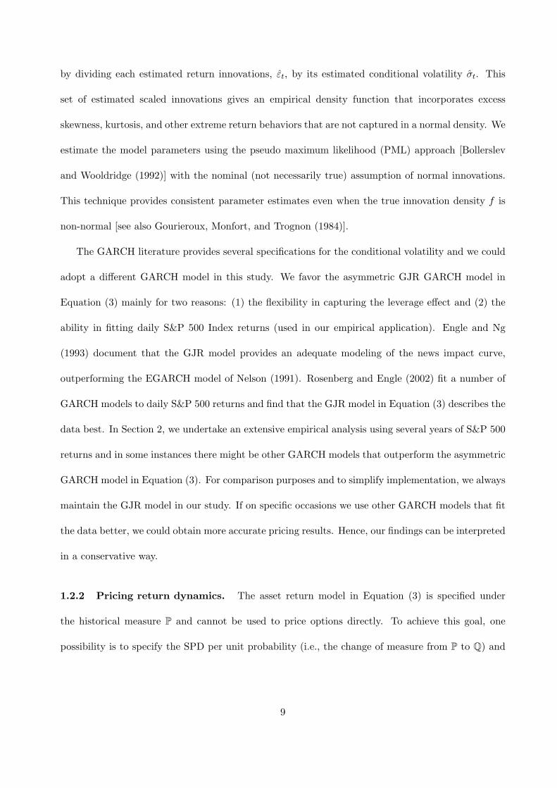
by dividing each estimated return innovations, εt, by its estimated conditional volatility σt. This

set of estimated scaled innovations gives an empirical density function that incorporates excess

skewness, kurtosis, and other extreme return behaviors that are not captured in a normal density. We

estimate the model parameters using the pseudo maximum likelihood (PML) approach [Bollerslev

and Wooldridge (1992)] with the nominal (not necessarily true) assumption of normal innovations.

This technique provides consistent parameter estimates even when the true innovation density f is

non-normal [see also Gourieroux, Monfort, and Trognon (1984)].

The GARCH literature provides several specifications for the conditional volatility and we could

adopt a different GARCH model in this study. We favor the asymmetric GJR GARCH model in

Equation (3) mainly for two reasons: (1) the flexibility in capturing the leverage effect and (2) the

ability in fitting daily S&P 500 Index returns (used in our empirical application). Engle and Ng

(1993) document that the GJR model provides an adequate modeling of the news impact curve,

outperforming the EGARCH model of Nelson (1991). Rosenberg and Engle (2002) fit a number of

GARCH models to daily S&P 500 returns and find that the GJR model in Equation (3) describes the

data best. In Section 2, we undertake an extensive empirical analysis using several years of S&P 500

returns and in some instances there might be other GARCH models that outperform the asymmetric

GARCH model in Equation (3). For comparison purposes and to simplify implementation, we always

maintain the GJR model in our study. If on specific occasions we use other GARCH models that fit

the data better, we could obtain more accurate pricing results. Hence, our findings can be interpreted

in a conservative way.

1.2.2 Pricing return dynamics. The asset return model in Equation (3) is specified under

the historical measure P and cannot be used to price options directly. To achieve this goal, one

possibility is to specify the SPD per unit probability (i.e., the change of measure from P to Q) and

9

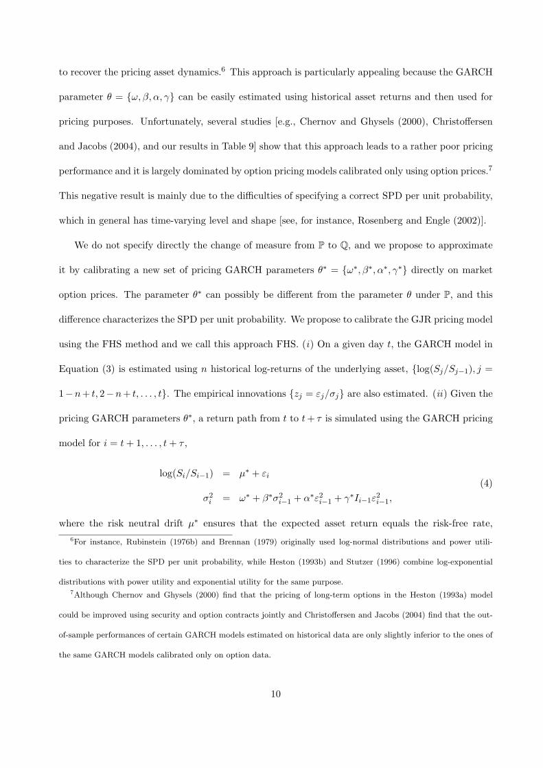
to recover the pricing asset dynamics.6 This approach is particularly appealing because the GARCH

parameter θ = {ω, β, α, γ} can be easily estimated using historical asset returns and then used for

pricing purposes. Unfortunately, several studies [e.g., Chernov and Ghysels (2000), Christoffersen

and Jacobs (2004), and our results in Table 9] show that this approach leads to a rather poor pricing

performance and it is largely dominated by option pricing models calibrated only using option prices.7

This negative result is mainly due to the difficulties of specifying a correct SPD per unit probability,

which in general has time-varying level and shape [see, for instance, Rosenberg and Engle (2002)].

We do not specify directly the change of measure from P to Q, and we propose to approximate

it by calibrating a new set of pricing GARCH parameters θ∗ = {ω∗, β∗, α∗, γ∗} directly on market

option prices. The parameter θ∗ can possibly be different from the parameter θ under P, and this

difference characterizes the SPD per unit probability. We propose to calibrate the GJR pricing model

using the FHS method and we call this approach FHS. (i) On a given day t, the GARCH model in

Equation (3) is estimated using n historical log-returns of the underlying asset, {log(Sj/Sj−1), j =

1−n+ t, 2−n+ t, . . . , t}. The empirical innovations {zj = εj/σj} are also estimated. (ii) Given the

pricing GARCH parameters θ∗, a return path from t to t+ τ is simulated using the GARCH pricing

model for i = t+ 1, . . . , t+ τ ,

log(Si/Si−1) = µ∗ + εi

σ2i = ω∗ + β∗σ2

i−1 + α∗ε2i−1 + γ∗Ii−1ε2i−1,

(4)

where the risk neutral drift µ∗ ensures that the expected asset return equals the risk-free rate,

6For instance, Rubinstein (1976b) and Brennan (1979) originally used log-normal distributions and power utili-

ties to characterize the SPD per unit probability, while Heston (1993b) and Stutzer (1996) combine log-exponential

distributions with power utility and exponential utility for the same purpose.7Although Chernov and Ghysels (2000) find that the pricing of long-term options in the Heston (1993a) model

could be improved using security and option contracts jointly and Christoffersen and Jacobs (2004) find that the out-

of-sample performances of certain GARCH models estimated on historical data are only slightly inferior to the ones of

the same GARCH models calibrated only on option data.

10

i.e., EQ[Si/Si−1|Fi−1] = er. A return path is simulated by drawing an estimated past innovation,

say, z[1], updating the conditional variance σ2t+1, drawing a second innovation z[2], updating the

conditional variance σ2t+2, and so on up to T = t + τ . The τ periods simulated return is ST /St =

exp(τµ∗ +∑τ

i=1 σt+i z[i]). (iii) The τ periods SPD is estimated by simulating several τ periods

return paths (i.e., repeating the previous step several times). (iv) The price of a call option at time t

with strike K and maturity T is given by e−rτ∑L

l=1 max(S(l)T −K, 0)/L, where S

(l)T is the simulated

asset price at time T in the l-th sample path and L is the total number of simulated sample paths

(e.g., L = 20,000). Put prices are computed similarly. (v) The pricing GARCH parameters θ∗ are

varied (which changes the sample paths) so as to best fit the cross section of option prices on date t,

minimizing the mean square pricing error∑Nt

j=1 e(Kj , Tj)2, where e(Kj , Tj) is the difference between

the GARCH model price and the market price of the option j with strike Kj and maturity Tj .8 Nt is

the number of options on a given day t. (vi) The calibration is achieved when, varying the pricing

GARCH parameter θ∗, the reduction in the mean square pricing error is negligible or below a given

threshold.

To reduce the Monte Carlo variance, we use the empirical martingale simulation method proposed

by Duan and Simonato (1998), where the simulated asset price paths are re-scaled to ensure that

the risk neutral expectation of the underlying asset equals its forward price. To lighten the notation,

σ2t denotes the pricing as well as the historical volatility, and it will be clear from the context which

volatility we are referring to. Similarly, εt denotes pricing and historical raw innovation.

The distribution of the scaled innovation z could also be changed to better approximate the

8To minimize the criterion function, we use the Nelder-Mead simplex direct search method implemented in the

Matlab function fminsearch, which does not require the computation of gradients. To ensure the convergence of the

calibration algorithm, the FHS innovations used to simulate the GARCH sample paths are kept fix across all the

iterations of the algorithm. Starting values for the pricing parameters θ∗ are the GARCH parameters estimated under

the historical measure P and obtained in the step (i).

11

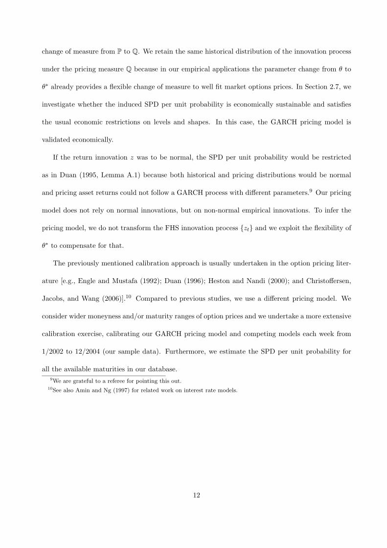
change of measure from P to Q. We retain the same historical distribution of the innovation process

under the pricing measure Q because in our empirical applications the parameter change from θ to

θ∗ already provides a flexible change of measure to well fit market options prices. In Section 2.7, we

investigate whether the induced SPD per unit probability is economically sustainable and satisfies

the usual economic restrictions on levels and shapes. In this case, the GARCH pricing model is

validated economically.

If the return innovation z was to be normal, the SPD per unit probability would be restricted

as in Duan (1995, Lemma A.1) because both historical and pricing distributions would be normal

and pricing asset returns could not follow a GARCH process with different parameters.9 Our pricing

model does not rely on normal innovations, but on non-normal empirical innovations. To infer the

pricing model, we do not transform the FHS innovation process {zt} and we exploit the flexibility of

θ∗ to compensate for that.

The previously mentioned calibration approach is usually undertaken in the option pricing liter-

ature [e.g., Engle and Mustafa (1992); Duan (1996); Heston and Nandi (2000); and Christoffersen,

Jacobs, and Wang (2006)].10 Compared to previous studies, we use a different pricing model. We

consider wider moneyness and/or maturity ranges of option prices and we undertake a more extensive

calibration exercise, calibrating our GARCH pricing model and competing models each week from

1/2002 to 12/2004 (our sample data). Furthermore, we estimate the SPD per unit probability for

all the available maturities in our database.

9We are grateful to a referee for pointing this out.10See also Amin and Ng (1997) for related work on interest rate models.

12

2 Empirical Analysis

2.1 Data

We use European options on the S&P 500 Index (symbol: SPX) to test our model. The market for

these options is one of the most active index options market in the world. Expiration months are the

three near-term months and three additional months from the March, June, September, December,

quarterly cycle. Strike price intervals are 5 and 25 points. The options are European and have no

wild card features. SPX options can be hedged using the active market on the S&P 500 futures.

Consequently, these options have been the focus of many empirical investigations, including Aıt-

Sahalia and Lo (1998), Chernov and Ghysels (2000), Heston and Nandi (2000), and Carr, Geman,

Madan, and Yor (2003).

We consider closing prices of the out-of-the-money (OTM) put and call SPX options for each

Wednesday11 from January 2, 2002 to December 29, 2004. It is known that OTM options are more

actively traded than in-the-money options and using only OTM options avoids the potential issues

associated with liquidity problems.12 Option data and all the other necessary data are downloaded

from OptionMetrics. The average of bid and ask prices are taken as option prices, while options

with time to maturity less than 10 days or more than 360 days, implied volatility larger than 70%,

or prices less than $0.05 are discarded, which yields a sample of 29,211 observations. Put and call

options are equally represented in the sample, which is 50.7% and 49.3%, respectively.

Using the term structure of zero-coupon default-free interest rates, the riskless interest rate for

each given maturity τ is obtained by linearly interpolating the two interest rates whose maturities

11In our sample, all but two days are Wednesdays. In those cases, we take the subsequent trading day, but for

simplicity we refer to all days as Wednesdays.12Daily volumes of out-of-the-money put options are usually several times as large as volumes of in-the-money puts.

This phenomenon started after the October 1987 crash and reflects the strong demand by portfolio managers for

protective puts, inducing implied volatility smiles.

13

straddle τ . This procedure is repeated for each contract and each day in the sample.

We divide the option data into several categories according to either time to maturity or mon-

eyness, m, defined as the ratio of the strike price over the asset price, K/S. A put option is said

to be deep out-of-the-money if its moneyness m < 0.85, or out-of-the-money if 0.85 ≤ m < 1. A

call option is said to be out-of-the-money if 1 ≤ m < 1.15; and deep out-of-the-money if m ≥ 1.15.

An option contract can be classified by the time to maturity: short maturity (< 60 days), medium

maturity (60–160 days), or long maturity (> 160 days).

Table 1 describes the 29,211 option prices, the implied volatilities, and the bid-ask spreads in

our database. The average put (call) prices range from $0.77 ($0.34) for short maturity, deep OTM

options to $38.80 ($34.82) for long maturity, OTM options. OTM put and call options account

for 27% and 25%, respectively, of the total sample. Short and long maturity options account for

33% and 36%, respectively, of the total sample. The table also shows the volatility smile and the

corresponding term structure. The smile across moneyness is evident for each given set of maturities.

When the time to maturity increases, the smile tends to become flatter and the bid-ask spreads tend

to narrow. The number of options on each Wednesday is on average 186.1, with a standard deviation

of 22.3, a minimum of 142, and a maximum of 237 option contracts.

During the sample period, the S&P 500 Index ranges from a minimum of $776.8 to a maximum

of $1,213.5, with an average level of $1,029.5. The average daily log-return is quite close to zero

(6.6 × 10−5), the standard deviation is 22.98% on an annual base,13 and skewness and kurtosis are

0.25 and 4.98 respectively.

13The standard deviation of the S&P 500 log-returns is approximately in line with the GARCH unconditional

volatility estimates reported in Tables 2 and 3.

14

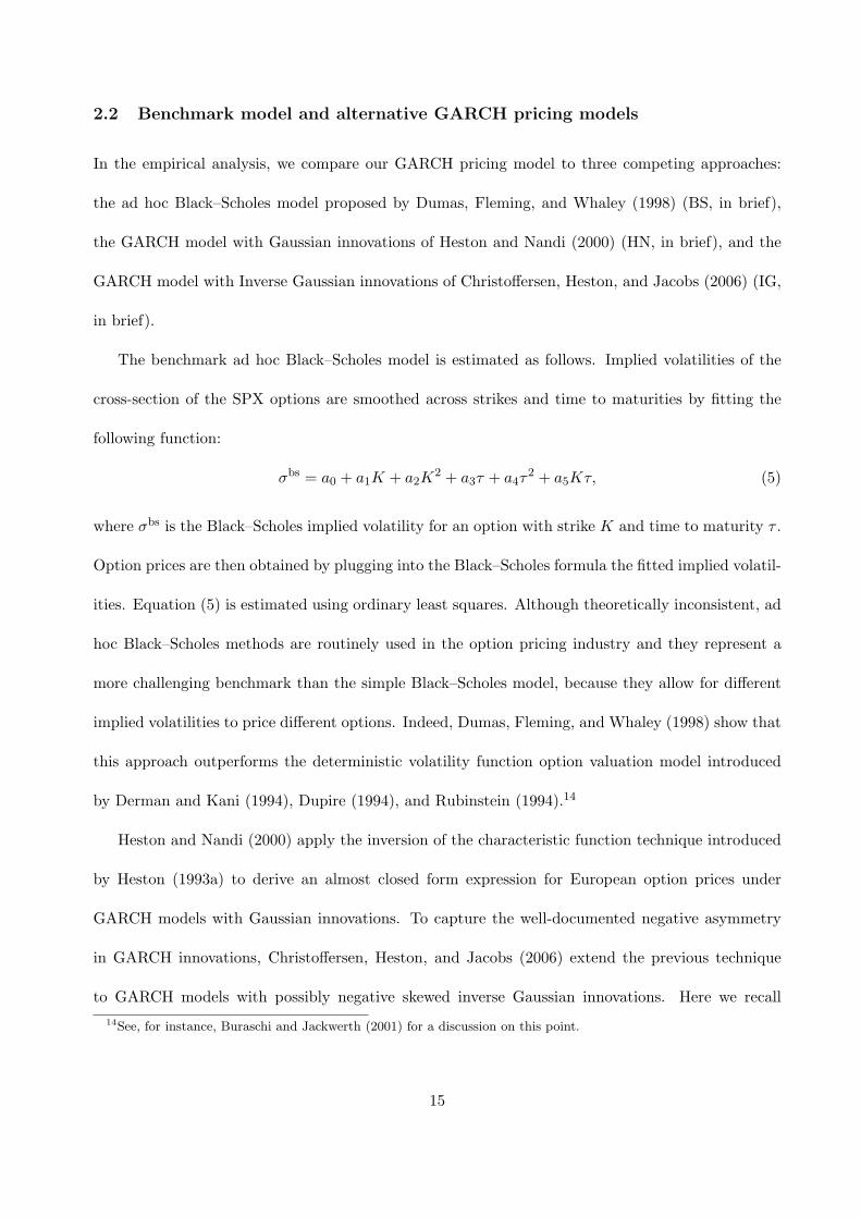
2.2 Benchmark model and alternative GARCH pricing models

In the empirical analysis, we compare our GARCH pricing model to three competing approaches:

the ad hoc Black–Scholes model proposed by Dumas, Fleming, and Whaley (1998) (BS, in brief),

the GARCH model with Gaussian innovations of Heston and Nandi (2000) (HN, in brief), and the

GARCH model with Inverse Gaussian innovations of Christoffersen, Heston, and Jacobs (2006) (IG,

in brief).

The benchmark ad hoc Black–Scholes model is estimated as follows. Implied volatilities of the

cross-section of the SPX options are smoothed across strikes and time to maturities by fitting the

following function:

σbs = a0 + a1K + a2K2 + a3τ + a4τ

2 + a5Kτ, (5)

where σbs is the Black–Scholes implied volatility for an option with strike K and time to maturity τ .

Option prices are then obtained by plugging into the Black–Scholes formula the fitted implied volatil-

ities. Equation (5) is estimated using ordinary least squares. Although theoretically inconsistent, ad

hoc Black–Scholes methods are routinely used in the option pricing industry and they represent a

more challenging benchmark than the simple Black–Scholes model, because they allow for different

implied volatilities to price different options. Indeed, Dumas, Fleming, and Whaley (1998) show that

this approach outperforms the deterministic volatility function option valuation model introduced

by Derman and Kani (1994), Dupire (1994), and Rubinstein (1994).14

Heston and Nandi (2000) apply the inversion of the characteristic function technique introduced

by Heston (1993a) to derive an almost closed form expression for European option prices under

GARCH models with Gaussian innovations. To capture the well-documented negative asymmetry

in GARCH innovations, Christoffersen, Heston, and Jacobs (2006) extend the previous technique

to GARCH models with possibly negative skewed inverse Gaussian innovations. Here we recall

14See, for instance, Buraschi and Jackwerth (2001) for a discussion on this point.

15

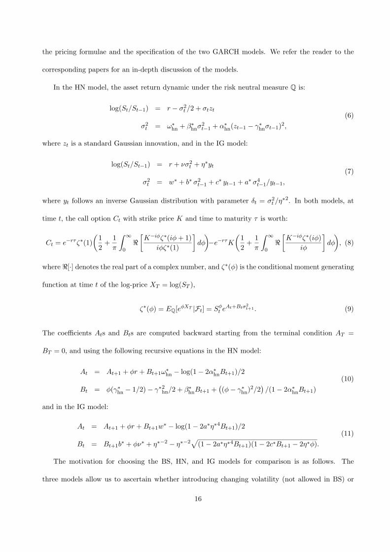
the pricing formulae and the specification of the two GARCH models. We refer the reader to the

corresponding papers for an in-depth discussion of the models.

In the HN model, the asset return dynamic under the risk neutral measure Q is:

log(St/St−1) = r − σ2t /2 + σtzt

σ2t = ω∗

hn + β∗hnσ2t−1 + α∗

hn(zt−1 − γ∗hnσt−1)2,

(6)

where zt is a standard Gaussian innovation, and in the IG model:

log(St/St−1) = r + νσ2t + η∗yt

σ2t = w∗ + b∗ σ2

t−1 + c∗ yt−1 + a∗ σ4t−1/yt−1,

(7)

where yt follows an inverse Gaussian distribution with parameter δt = σ2t /η

∗2. In both models, at

time t, the call option Ct with strike price K and time to maturity τ is worth:

Ct = e−rτζ∗(1)

(

1

2+

1

π

∫ ∞

0ℜ

[

K−iφζ∗(iφ+ 1)

iφζ∗(1)

]

dφ

)

−e−rτK

(

1

2+

1

π

∫ ∞

0ℜ

[

K−iφζ∗(iφ)

iφ

]

dφ

)

, (8)

where ℜ[·] denotes the real part of a complex number, and ζ∗(φ) is the conditional moment generating

function at time t of the log-price XT = log(ST ),

ζ∗(φ) = EQ[eφXT |Ft] = Sφt e

At+Btσ2t+1 . (9)

The coefficients Ats and Bts are computed backward starting from the terminal condition AT =

BT = 0, and using the following recursive equations in the HN model:

At = At+1 + φr +Bt+1ω∗hn − log(1 − 2α∗

hnBt+1)/2

Bt = φ(γ∗hn − 1/2) − γ∗2hn/2 + β∗hnBt+1 +

(

(φ− γ∗hn)2/2

)

/(1 − 2α∗hnBt+1)

(10)

and in the IG model:

At = At+1 + φr +Bt+1w∗ − log(1 − 2a∗η∗4Bt+1)/2

Bt = Bt+1b∗ + φν∗ + η∗−2 − η∗−2

√

(1 − 2a∗η∗4Bt+1)(1 − 2c∗Bt+1 − 2η∗φ).

(11)

The motivation for choosing the BS, HN, and IG models for comparison is as follows. The

three models allow us to ascertain whether introducing changing volatility (not allowed in BS) or

16

non-normality (not allowed in BS and HN) leads to better pricing using our FHS approach. The

comparison between the IG and FHS models concerns the relative advantage of modeling non-

normality of innovations parametrically or in a nonparametric way, respectively.

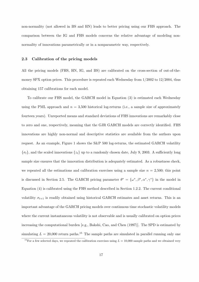
2.3 Calibration of the pricing models

All the pricing models (FHS, HN, IG, and BS) are calibrated on the cross-section of out-of-the-

money SPX option prices. This procedure is repeated each Wednesday from 1/2002 to 12/2004, thus

obtaining 157 calibrations for each model.

To calibrate our FHS model, the GARCH model in Equation (3) is estimated each Wednesday

using the PML approach and n = 3,500 historical log-returns (i.e., a sample size of approximately

fourteen years). Unreported means and standard deviations of FHS innovations are remarkably close

to zero and one, respectively, meaning that the GJR GARCH models are correctly identified. FHS

innovations are highly non-normal and descriptive statistics are available from the authors upon

request. As an example, Figure 1 shows the S&P 500 log-returns, the estimated GARCH volatility

{σt}, and the scaled innovations {zt} up to a randomly chosen date, July 9, 2003. A sufficiently long

sample size ensures that the innovation distribution is adequately estimated. As a robustness check,

we repeated all the estimations and calibration exercises using a sample size n = 2,500; this point

is discussed in Section 2.5. The GARCH pricing parameter θ∗ = {ω∗, β∗, α∗, γ∗} in the model in

Equation (4) is calibrated using the FHS method described in Section 1.2.2. The current conditional

volatility σt+1 is readily obtained using historical GARCH estimates and asset returns. This is an

important advantage of the GARCH pricing models over continuous time stochastic volatility models

where the current instantaneous volatility is not observable and is usually calibrated on option prices

increasing the computational burden [e.g., Bakshi, Cao, and Chen (1997)]. The SPD is estimated by

simulating L = 20,000 return paths.15 The sample paths are simulated in parallel running only one

15For a few selected days, we repeated the calibration exercises using L = 10,000 sample paths and we obtained very

17

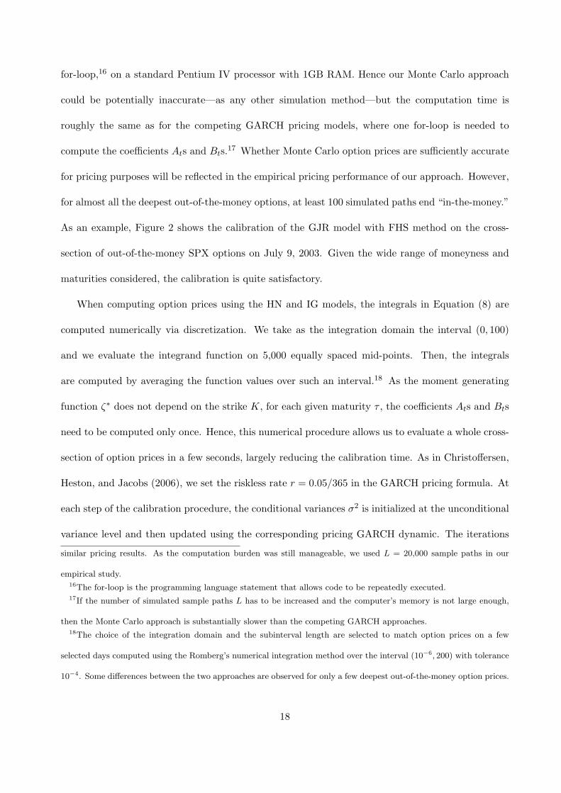
for-loop,16 on a standard Pentium IV processor with 1GB RAM. Hence our Monte Carlo approach

could be potentially inaccurate—as any other simulation method—but the computation time is

roughly the same as for the competing GARCH pricing models, where one for-loop is needed to

compute the coefficients Ats and Bts.17 Whether Monte Carlo option prices are sufficiently accurate

for pricing purposes will be reflected in the empirical pricing performance of our approach. However,

for almost all the deepest out-of-the-money options, at least 100 simulated paths end “in-the-money.”

As an example, Figure 2 shows the calibration of the GJR model with FHS method on the cross-

section of out-of-the-money SPX options on July 9, 2003. Given the wide range of moneyness and

maturities considered, the calibration is quite satisfactory.

When computing option prices using the HN and IG models, the integrals in Equation (8) are

computed numerically via discretization. We take as the integration domain the interval (0, 100)

and we evaluate the integrand function on 5,000 equally spaced mid-points. Then, the integrals

are computed by averaging the function values over such an interval.18 As the moment generating

function ζ∗ does not depend on the strike K, for each given maturity τ , the coefficients Ats and Bts

need to be computed only once. Hence, this numerical procedure allows us to evaluate a whole cross-

section of option prices in a few seconds, largely reducing the calibration time. As in Christoffersen,

Heston, and Jacobs (2006), we set the riskless rate r = 0.05/365 in the GARCH pricing formula. At

each step of the calibration procedure, the conditional variances σ2 is initialized at the unconditional

variance level and then updated using the corresponding pricing GARCH dynamic. The iterations

similar pricing results. As the computation burden was still manageable, we used L = 20,000 sample paths in our

empirical study.16The for-loop is the programming language statement that allows code to be repeatedly executed.17If the number of simulated sample paths L has to be increased and the computer’s memory is not large enough,

then the Monte Carlo approach is substantially slower than the competing GARCH approaches.18The choice of the integration domain and the subinterval length are selected to match option prices on a few

selected days computed using the Romberg’s numerical integration method over the interval (10−6, 200) with tolerance

10−4. Some differences between the two approaches are observed for only a few deepest out-of-the-money option prices.

18

are started 250 trading days before the first option date to allow for the models to find the right

conditional variances.

Christoffersen, Heston, and Jacobs (2006) show that the ν∗ parameter in the IG model is not a

free parameter but it is constrained to ensure that the underlying asset earns the risk-free rate under

the risk neutral measure Q. This observation explains why ν∗ does not appear in Table 3, which

shows the calibrated risk neutral parameters.

Finally, when implementing all the pricing formulae, the dividends paid by the stocks in the

S&P 500 Index have to be taken into account. Dividends are treated in different ways in option

pricing literature [e.g., Aıt-Sahalia and Lo (1998) and Heston and Nandi (2000) for two alternative

procedures]. We use the dividend yields downloaded from OptionMetrics to compute an ex-dividend

spot index level.

2.4 In-sample model comparison

Table 3 shows summary statistics for the pricing GARCH parameters calibrated each Wednesday

from 1/2002 to 12/2004. It is known that option prices are more sensitive, for example, to γ∗,

γ∗hn, c∗, and η∗ than ω∗, ω∗

hn, or w∗. Indeed, the first set of parameters turns out to be more

stable than the second one, confirming the finding, for instance, in Heston and Nandi (2000). As

expected, all the unconditional volatilities and the corresponding persistency measures are more

stable than single parameters. For each Wednesday, we also calibrate the ad hoc Black–Scholes model

in Equation (5). Table 4 shows summary statistics for the parameter estimates ai, i = 0, . . . , 5. The

low standard deviations of the parameter estimates confirm that the implied volatility smile is a

persistent phenomenon in the SPX option market.

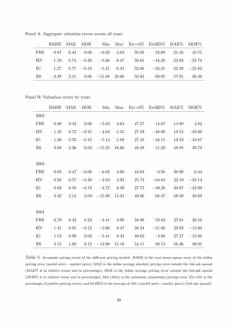
Following Dumas, Fleming, and Whaley (1998) and Heston and Nandi (2000), in order to assess

the quality of the pricing models, we report several measurements of fit. The dollar root mean square

error (RMSE), i.e., the square root of the averaged squared deviations between the model prices and

19

the market prices; the mean absolute error (MAE), i.e., the average of the absolute valuation error

when the model price is outside the bid-ask spread; the mean outside error (MOE), i.e., the average of

the valuation error when the model price is outside the bid-ask spread; the minimum and maximum

pricing errors; the percentage of positive pricing errors; and the average pricing error as a percentage

of the bid-ask spread.

For all pricing models, Table 5 shows the in-sample pricing errors summarized by the previous

measurements of fit. Table 6 disaggregates the in-sample pricing errors by moneyness/maturity

categories; see also the left graphs in Figure 3 for the in-sample absolute mispricing. The overall

conclusion is that, in terms of all measurements of fit, our GJR model with FHS innovations out-

performs all the other pricing models. For example, the aggregate RMSE of the IG and HN models

are 46% and 37% larger than the RMSE of our FHS model. Occasionally, the GJR is somewhat

outperformed by other models (e.g., in terms of RMSE by the HN model during 2003 in Table 5, or

by the IG model for deep out-of-the-money put options in Table 6), but its good pricing performance

is remarkably stable. The percentage of positive pricing errors in Table 5 for the HN and the IG

models seems to be too low, but no systematic bias emerges for the MOEs in Table 6 and hence this

finding is due to slight underestimations of option prices. Finally, all the GARCH pricing models

largely outperform the benchmark ad hoc Black–Scholes model, which has difficulties in fitting the

whole cross-section of option prices. As a further comparison, we also consider the CGMY models

proposed by Carr, Geman, Madan, and Yor (2003), where the underlying asset follows a mean cor-

rected, time-changed exponential Levy process. Despite their models having more parameters (e.g.,

the CGMYSA model has nine parameters), our FHS model compares favorably. To save space, the

corresponding results are omitted but are available from the authors upon request.

20

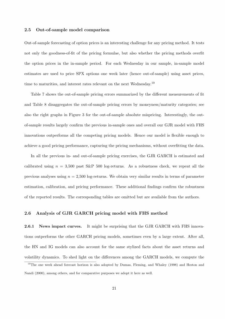
2.5 Out-of-sample model comparison

Out-of-sample forecasting of option prices is an interesting challenge for any pricing method. It tests

not only the goodness-of-fit of the pricing formulae, but also whether the pricing methods overfit

the option prices in the in-sample period. For each Wednesday in our sample, in-sample model

estimates are used to price SPX options one week later (hence out-of-sample) using asset prices,

time to maturities, and interest rates relevant on the next Wednesday.19

Table 7 shows the out-of-sample pricing errors summarized by the different measurements of fit

and Table 8 disaggregates the out-of-sample pricing errors by moneyness/maturity categories; see

also the right graphs in Figure 3 for the out-of-sample absolute mispricing. Interestingly, the out-

of-sample results largely confirm the previous in-sample ones and overall our GJR model with FHS

innovations outperforms all the competing pricing models. Hence our model is flexible enough to

achieve a good pricing performance, capturing the pricing mechanisms, without overfitting the data.

In all the previous in- and out-of-sample pricing exercises, the GJR GARCH is estimated and

calibrated using n = 3,500 past S&P 500 log-returns. As a robustness check, we repeat all the

previous analyses using n = 2,500 log-returns. We obtain very similar results in terms of parameter

estimation, calibration, and pricing performance. These additional findings confirm the robustness

of the reported results. The corresponding tables are omitted but are available from the authors.

2.6 Analysis of GJR GARCH pricing model with FHS method

2.6.1 News impact curves. It might be surprising that the GJR GARCH with FHS innova-

tions outperforms the other GARCH pricing models, sometimes even by a large extent. After all,

the HN and IG models can also account for the same stylized facts about the asset returns and

volatility dynamics. To shed light on the differences among the GARCH models, we compute the

19The one week ahead forecast horizon is also adopted by Dumas, Fleming, and Whaley (1998) and Heston and

Nandi (2000), among others, and for comparative purposes we adopt it here as well.

21

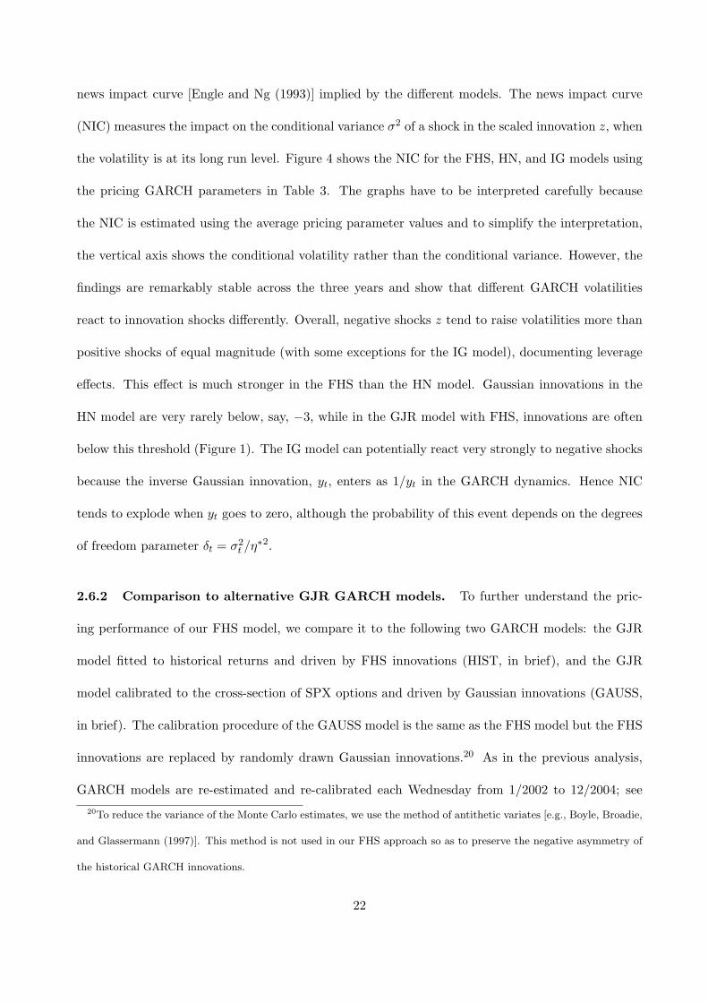
news impact curve [Engle and Ng (1993)] implied by the different models. The news impact curve

(NIC) measures the impact on the conditional variance σ2 of a shock in the scaled innovation z, when

the volatility is at its long run level. Figure 4 shows the NIC for the FHS, HN, and IG models using

the pricing GARCH parameters in Table 3. The graphs have to be interpreted carefully because

the NIC is estimated using the average pricing parameter values and to simplify the interpretation,

the vertical axis shows the conditional volatility rather than the conditional variance. However, the

findings are remarkably stable across the three years and show that different GARCH volatilities

react to innovation shocks differently. Overall, negative shocks z tend to raise volatilities more than

positive shocks of equal magnitude (with some exceptions for the IG model), documenting leverage

effects. This effect is much stronger in the FHS than the HN model. Gaussian innovations in the

HN model are very rarely below, say, −3, while in the GJR model with FHS, innovations are often

below this threshold (Figure 1). The IG model can potentially react very strongly to negative shocks

because the inverse Gaussian innovation, yt, enters as 1/yt in the GARCH dynamics. Hence NIC

tends to explode when yt goes to zero, although the probability of this event depends on the degrees

of freedom parameter δt = σ2t /η

∗2.

2.6.2 Comparison to alternative GJR GARCH models. To further understand the pric-

ing performance of our FHS model, we compare it to the following two GARCH models: the GJR

model fitted to historical returns and driven by FHS innovations (HIST, in brief), and the GJR

model calibrated to the cross-section of SPX options and driven by Gaussian innovations (GAUSS,

in brief). The calibration procedure of the GAUSS model is the same as the FHS model but the FHS

innovations are replaced by randomly drawn Gaussian innovations.20 As in the previous analysis,

GARCH models are re-estimated and re-calibrated each Wednesday from 1/2002 to 12/2004; see

20To reduce the variance of the Monte Carlo estimates, we use the method of antithetic variates [e.g., Boyle, Broadie,

and Glassermann (1997)]. This method is not used in our FHS approach so as to preserve the negative asymmetry of

the historical GARCH innovations.

22

Table 2 for GARCH parameters of HIST and GAUSS models. Table 9 shows in- and out-of-sample

aggregated pricing results; to simplify comparisons, pricing results of the HN and FHS models are

reported in this table as well. Comparing FHS and HIST models (which rely on the same FHS inno-

vation distribution but different asset return dynamics) shows that allowing for different historical

and pricing return distributions induces a major improvement in the pricing performance, such as a

reduction of more than 70% in terms of RMSE. Comparing FHS and GAUSS models (which rely on

the same GARCH dynamic but different innovation distributions) shows that using nonparametric

instead of Gaussian innovations induces an overall improvement in pricing options, but by a lesser

extent. Finally, comparing GAUSS and HN models (which rely on different GARCH dynamics but

the same Gaussian innovation distribution) shows that the GJR GARCH dynamic allows for a better

fitting of option prices than the asymmetric GARCH dynamic in Heston and Nandi (2000). Pricing

errors disaggregated across years and moneyness/maturity categories confirm the results in Table 9

and are omitted, but are available from the authors upon request.

Overall, allowing for different volatilities (and hence different distributions) under historical and

pricing measures induces a major improvement in the pricing performance. This finding is in line

with recent studies on variance swap contracts, which document higher risk neutral volatilities than

historical ones, inducing negative volatility premia [e.g., Carr and Wu (2008); and Egloff, Leippold,

and Wu (2007)]. Capturing this phenomenon seems to be crucial in order to achieve accurate pricing

performances.

2.6.3 Applications of GJR GARCH pricing model with FHS method. The proposed

GARCH pricing model has been used to price European calls and puts but the model has other

potential applications as well. As the calibration procedure relies on Monte Carlo simulation, tran-

sition densities of the stock price are readily available. Hence other European and path-dependent

claims can be priced and hedged using the simulated trajectories of the stock price. In particular,

23

a sensitivity analysis (e.g., computing delta and gamma) can be easily obtained following the direct

approach in Duan (1995) or the regression methodology approach in Longstaff and Schwartz (2001).

Recently, Barone-Adesi and Elliott (2007) proposed a model-free approach to computing delta hedge

ratios. Comparing option price forecasts based on their model-free approach and on our GARCH

model allows to evaluate the deterioration of delta hedging due to volatility shocks.

Our GARCH pricing model provides an arbitrage-free procedure to optimally interpolate strike

prices and time to maturities, as required in several applications.21 In particular, the grid of time to

maturities is rather sparse and standard interpolation methods are likely not to work in that case.

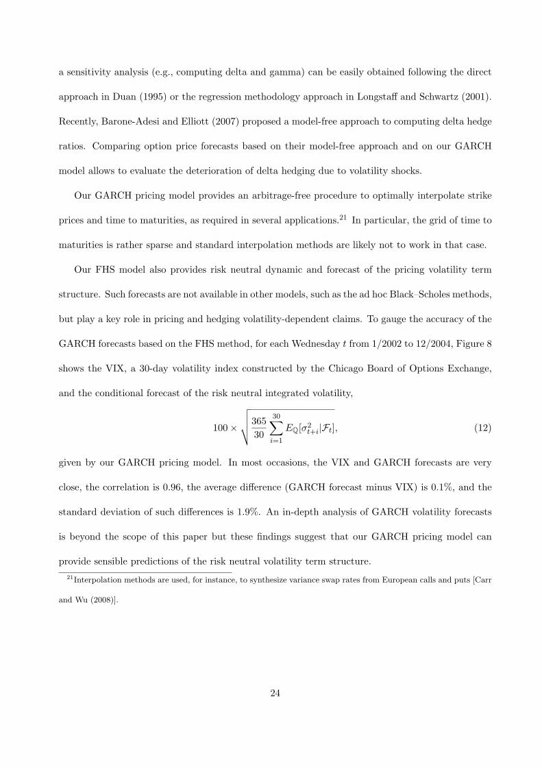
Our FHS model also provides risk neutral dynamic and forecast of the pricing volatility term

structure. Such forecasts are not available in other models, such as the ad hoc Black–Scholes methods,

but play a key role in pricing and hedging volatility-dependent claims. To gauge the accuracy of the

GARCH forecasts based on the FHS method, for each Wednesday t from 1/2002 to 12/2004, Figure 8

shows the VIX, a 30-day volatility index constructed by the Chicago Board of Options Exchange,

and the conditional forecast of the risk neutral integrated volatility,

100 ×

√

√

√

√

365

30

30∑

i=1

EQ[σ2t+i|Ft], (12)

given by our GARCH pricing model. In most occasions, the VIX and GARCH forecasts are very

close, the correlation is 0.96, the average difference (GARCH forecast minus VIX) is 0.1%, and the

standard deviation of such differences is 1.9%. An in-depth analysis of GARCH volatility forecasts

is beyond the scope of this paper but these findings suggest that our GARCH pricing model can

provide sensible predictions of the risk neutral volatility term structure.

21Interpolation methods are used, for instance, to synthesize variance swap rates from European calls and puts [Carr

and Wu (2008)].

24

2.7 State price density per unit probability

In this section, we estimate SPD per unit probability, Mt,t+τ , using our FHS model (Section 1.2) and

the GAUSS model (Section 2.6.2), and we study their economic implications. Estimates of Mt,t+τ

are based on conditional historical and pricing densities, pt,t+τ and qt,t+τ . In our FHS model, the

historical density pt,t+τ is obtained by simulating from t to t+ τ the GJR model fitted to historical

log-returns up to time t and driven by FHS innovations.22 The historical density depends on the

expected return, which is notoriously difficult to estimate. Indeed, Merton (1980) argues that positive

risk premia should be explicitly modeled and, as in Jackwerth (2000), we set the risk premium at 8%

per year. The pricing density qt,t+τ is obtained by simulating the GJR model calibrated on the cross-

section of SPX options observed on date t and driven by the same FHS innovations. Then, Mt,t+τ is

given by the discounted ratio of the pricing over the historical densities, Mt,t+τ = e−rτqt,t+τ/pt,t+τ .

This procedure gives semiparametric estimates of Mt,t+τ , because the densities pt,t+τ and qt,t+τ are

based on parametric GARCH models, but no a priori functional form is imposed on Mt,t+τ . In the

GAUSS model, the estimation procedure of Mt,t+τ is the same as for the FHS model but the FHS

innovations are replaced by Gaussian innovations.

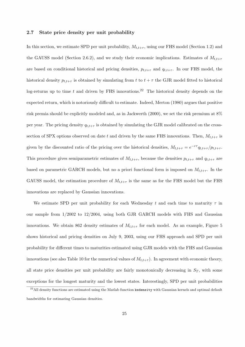
We estimate SPD per unit probability for each Wednesday t and each time to maturity τ in

our sample from 1/2002 to 12/2004, using both GJR GARCH models with FHS and Gaussian

innovations. We obtain 862 density estimates of Mt,t+τ for each model. As an example, Figure 5

shows historical and pricing densities on July 9, 2003, using our FHS approach and SPD per unit

probability for different times to maturities estimated using GJR models with the FHS and Gaussian

innovations (see also Table 10 for the numerical values ofMt,t+τ ). In agreement with economic theory,

all state price densities per unit probability are fairly monotonically decreasing in ST , with some

exceptions for the longest maturity and the lowest states. Interestingly, SPD per unit probabilities

22All density functions are estimated using the Matlab function ksdensity with Gaussian kernels and optimal default

bandwidths for estimating Gaussian densities.

25

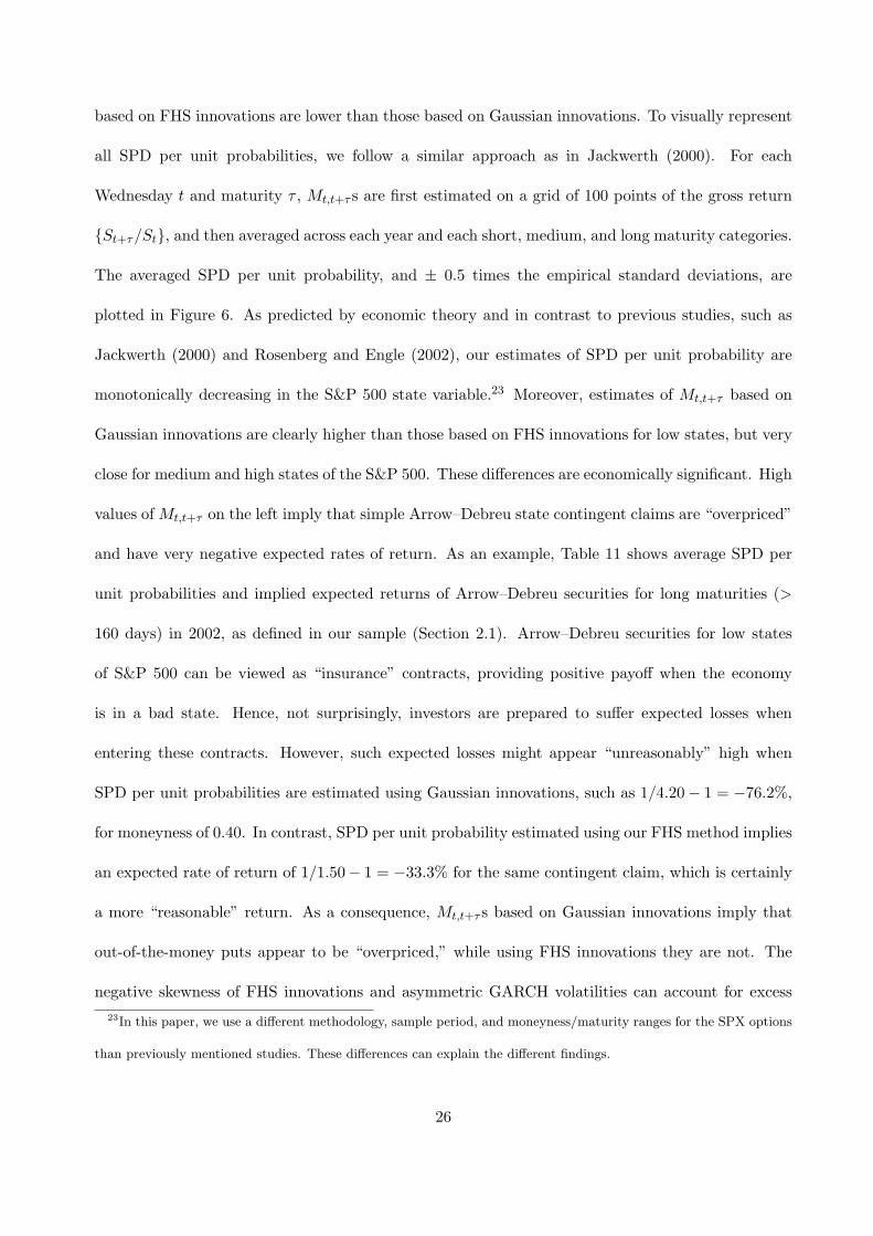
based on FHS innovations are lower than those based on Gaussian innovations. To visually represent

all SPD per unit probabilities, we follow a similar approach as in Jackwerth (2000). For each

Wednesday t and maturity τ , Mt,t+τ s are first estimated on a grid of 100 points of the gross return

{St+τ/St}, and then averaged across each year and each short, medium, and long maturity categories.

The averaged SPD per unit probability, and ± 0.5 times the empirical standard deviations, are

plotted in Figure 6. As predicted by economic theory and in contrast to previous studies, such as

Jackwerth (2000) and Rosenberg and Engle (2002), our estimates of SPD per unit probability are

monotonically decreasing in the S&P 500 state variable.23 Moreover, estimates of Mt,t+τ based on

Gaussian innovations are clearly higher than those based on FHS innovations for low states, but very

close for medium and high states of the S&P 500. These differences are economically significant. High

values of Mt,t+τ on the left imply that simple Arrow–Debreu state contingent claims are “overpriced”

and have very negative expected rates of return. As an example, Table 11 shows average SPD per

unit probabilities and implied expected returns of Arrow–Debreu securities for long maturities (>

160 days) in 2002, as defined in our sample (Section 2.1). Arrow–Debreu securities for low states

of S&P 500 can be viewed as “insurance” contracts, providing positive payoff when the economy

is in a bad state. Hence, not surprisingly, investors are prepared to suffer expected losses when

entering these contracts. However, such expected losses might appear “unreasonably” high when

SPD per unit probabilities are estimated using Gaussian innovations, such as 1/4.20 − 1 = −76.2%,

for moneyness of 0.40. In contrast, SPD per unit probability estimated using our FHS method implies

an expected rate of return of 1/1.50− 1 = −33.3% for the same contingent claim, which is certainly

a more “reasonable” return. As a consequence, Mt,t+τ s based on Gaussian innovations imply that

out-of-the-money puts appear to be “overpriced,” while using FHS innovations they are not. The

negative skewness of FHS innovations and asymmetric GARCH volatilities can account for excess

23In this paper, we use a different methodology, sample period, and moneyness/maturity ranges for the SPX options

than previously mentioned studies. These differences can explain the different findings.

26

out-of-the-money put prices and provide an adequate pricing of the downside market risk.

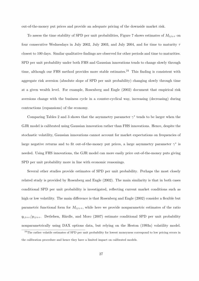
To assess the time stability of SPD per unit probabilities, Figure 7 shows estimates of Mt,t+τ on

four consecutive Wednesdays in July 2002, July 2003, and July 2004, and for time to maturity τ

closest to 100 days. Similar qualitative findings are observed for other periods and time to maturities.

SPD per unit probability under both FHS and Gaussian innovations tends to change slowly through

time, although our FHS method provides more stable estimates.24 This finding is consistent with

aggregate risk aversion (absolute slope of SPD per unit probability) changing slowly through time

at a given wealth level. For example, Rosenberg and Engle (2002) document that empirical risk

aversions change with the business cycle in a counter-cyclical way, increasing (decreasing) during

contractions (expansions) of the economy.

Comparing Tables 2 and 3 shows that the asymmetry parameter γ∗ tends to be larger when the

GJR model is calibrated using Gaussian innovation rather than FHS innovations. Hence, despite the

stochastic volatility, Gaussian innovations cannot account for market expectations on frequencies of

large negative returns and to fit out-of-the-money put prices, a large asymmetry parameter γ∗ is

needed. Using FHS innovations, the GJR model can more easily price out-of-the-money puts giving

SPD per unit probability more in line with economic reasonings.

Several other studies provide estimates of SPD per unit probability. Perhaps the most closely

related study is provided by Rosenberg and Engle (2002). The main similarity is that in both cases

conditional SPD per unit probability is investigated, reflecting current market conditions such as

high or low volatility. The main difference is that Rosenberg and Engle (2002) consider a flexible but

parametric functional form for Mt,t+τ , while here we provide nonparametric estimates of the ratio

qt,t+τ/pt,t+τ . Detlefsen, Hardle, and Moro (2007) estimate conditional SPD per unit probability

nonparametrically using DAX options data, but relying on the Heston (1993a) volatility model.

24The rather volatile estimates of SPD per unit probability for lowest moneyness correspond to low pricing errors in

the calibration procedure and hence they have a limited impact on calibrated models.

27

Aıt-Sahalia and Lo (2000) and Jackwerth (2000) provide nonparametric estimates of SPD per unit

probability (or related quantities such as risk aversions), but they exploit the time continuity of

Mt,t+τ to average state prices and probabilities across time. Hence, their results are best interpreted

as estimates of the average SPD per unit probability over the sample period, instead of conditional

estimates; for a recent extension see Constantinides, Jackwerth, and Perrakis (2008). Compared

to all the previous studies, we provide estimates of SPD per unit probability for many more time

horizons τ and much larger ranges of St+τ/St.

3 Conclusions

We propose a new method for pricing options based on an asymmetric GARCH model with filtered

historical innovations. In an incomplete market framework, we allow for historical and pricing dis-

tributions to have different shapes, enhancing the model flexibility to fit market option prices. An

extensive empirical analysis based on S&P 500 Index options shows that our model outperforms other

competing GARCH pricing models and ad hoc Black–Scholes methods. We show that the flexible

change of measure, the asymmetric GARCH volatility dynamic, and the nonparametric innovation

distribution induce the accurate pricing performance of our model. In contrast to previous studies,

using our GARCH model and a nonparametric approach we obtain decreasing state price densi-

ties per unit probability as suggested by economic theory, therefore validating our GARCH pricing

model. Furthermore, implied volatility smiles appear to be explained by asymmetric GARCH volatil-

ity and negative skewness of the filtered historical innovations, with no need for “unreasonably” high

state prices for out-of-the-money puts. Our discrete-time model does not impose restrictions similar

to Girsanov’s theorem on the change of measure. The only requirement is the non-negativity of

state prices, which are necessary for no arbitrage and ensured by our Monte Carlo method. Such a

weak requirement allows for more flexible option pricing than enabled by diffusion models. Further

28

refinements of pricing and stability issues are left to future research.

References

Aıt-Sahalia, Y., and A. W. Lo, 1998, “Nonparametric Estimation of State-price Densities Implicit in

Financial Assets Prices,” Journal of Finance, 53, 499–548.

, 2000, “Nonparametric Risk Management and Implied Risk Aversion,” Journal of Econo-

metrics, 94, 9–51.

Amin, K. I., and V. K. Ng, 1997, “Inferring Future Volatility from the Information in Implied

Volatility in Eurodollar Options: A New Approach,” Review of Financial Studies, 10, 333–367.

Arrow, K., 1964, “The Role of Securities in the Optimal Allocation of Risk Bearing,” Review of

Economic Studies, 31, 91–96.

Bakshi, G., C. Cao, and Z. Chen, 1997, “Empirical Performance of Alternative Option Pricing

Models,” Journal of Finance, 52, 2003–2049.

Barone-Adesi, G., F. Bourgoin, and K. Giannopoulos, 1998, “Don’t Look Back,” Risk, 11, 100–103.

Barone-Adesi, G., and R. J. Elliott, 2007, “Cutting the Hedge,” Computational Economics, 29,

151–158.

Bekaert, G., and G. Wu, 2000, “Asymmetric Volatility and Risk in Equity Markets,” Review of

Financial Studies, 13, 1–42.

Black, F., 1976, “Studies of Stock Market Volatility Changes,” in Proceedings of the 1976 Meetings

of the American Statistical Association, Business and Economic Statistic Section, 177–181.

Black, F., and M. Scholes, 1973, “The Valuation of Options and Corporate Liabilities,” Journal of

Political Economy, 81, 637–654.

29

Bollerslev, T., 1986, “Generalized Autoregressive Conditional Heteroskedasticity,” Journal of Econo-

metrics, 31, 307–327.

Bollerslev, T., R. Y. Chou, and K. F. Kroner, 1992, “ARCH Modeling in Finance—A Review of the

Theory and Empirical Evidence,” Journal of Econometrics, 52, 5–59.

Bollerslev, T., R. F. Engle, and D. B. Nelson, 1994, “ARCH Models,” in Handbook of Econometrics,

ed. by R. F. Engle, and D. L. McFadden. North-Holland, Amsterdam, 2959–3038.

Bollerslev, T., and J. M. Wooldridge, 1992, “Quasi-maximum Likelihood Estimation and Inference

in Dynamic Models with Time Varying Covariances,” Econometric Reviews, 11, 143–172.

Boyle, P., M. Broadie, and P. Glassermann, 1997, “Monte Carlo Methods for Security Pricing,”

Journal of Economic Dynamics and Control, 21, 1267–1321.

Brennan, M. J., 1979, “The Pricing of Contingent Claims in Discrete Time Models,” Journal of

Finance, 34, 53–68.

Brown, D. P., and M. R. Gibbons, 1985, “A Simple Econometric Approach for Utility-based Asset

Pricing Models,” Journal of Finance, 40, 359–381.

Buraschi, A., and J. C. Jackwerth, 2001, “The Price of a Smile: Hedging and Spanning in Option

Markets,” Review of Financial Studies, 14, 495–527.

Campbell, J. Y., and L. Hentschel, 1992, “No News Is Good News: An Asymmetric Model of

Changing Volatility in Stock Returns,” Journal of Financial Economics, 31, 281–318.

Campbell, J. Y., A. W. Lo, and C. MacKinlay, 1997, The Econometrics of Financial Markets.

Princeton University Press, Princeton, NJ.

Carr, P., H. Geman, D. B. Madan, and M. Yor, 2003, “Stochastic Volatility for Levy Processes,”

Mathematical Finance, 13, 345–382.

30

Carr, P., and L. Wu, 2008, “Variance Risk Premia,” Review of Financial Studies, forthcoming.

Chernov, M., and E. Ghysels, 2000, “A Study Towards a Unified Approach to the Joint Estimation of

Objective and Risk Neutral Measures for the Purpose of Options Valuation,” Journal of Financial

Economics, 56, 407–458.

Christie, A., 1982, “The Stochastic Behavior of Common Stock Variances: Value, Leverage and

Interest Rate Effects,” Journal of Financial Economics, 10, 407–432.

Christoffersen, P., S. Heston, and K. Jacobs, 2006, “Option Valuation with Conditional Skewness,”

Journal of Econometrics, 131, 253–284.

Christoffersen, P., and K. Jacobs, 2004, “Which GARCH Model for Option Valuation?,” Management

Science, 50, 1204–1221.

Christoffersen, P., K. Jacobs, and Y. Wang, 2006, “Option Valuation with Long-run and Short-run

Volatility Components,” Working paper, McGill University, Canada.

Cochrane, J. H., 2001, Asset Pricing. Princeton University Press, Princeton, NJ.

Constantinides, G. M., J. C. Jackwerth, and S. Perrakis, 2008, “Mispricing of S&P 500 Index Op-

tions,” Review of Financial Studies, forthcoming.

Cox, J. C., and S. A. Ross, 1976, “The Valuation of Options for Alternative Stochastic Processes,”

Journal of Financial Economics, 3, 145–166.

Debreu, G., 1959, Theory of Value. Wiley, New York.

Derman, E., and I. Kani, 1994, “Riding on the Smile,” Risk, 7, 32–39.

Detlefsen, K., W. K. Hardle, and R. A. Moro, 2007, “Empirical Pricing Kernels and Investor Pref-

erences,” Working paper, Humboldt University of Berlin.

31

Duan, J.-C., 1995, “The GARCH Option Pricing Model,” Mathematical Finance, 5, 13–32.

, 1996, “Cracking the Smile,” Risk, 9, 55–59.

Duan, J.-C., and J.-G. Simonato, 1998, “Empirical Martingale Simulation for Asset Prices,” Man-

agement Science, 44, 1218–1233.

Dumas, B., J. Fleming, and R. E. Whaley, 1998, “Implied Volatility Functions: Empirical Tests,”

Journal of Finance, 53, 2059–2106.

Dupire, B., 1994, “Pricing with a Smile,” Risk, 7, 18–20.

Egloff, D., M. Leippold, and L. Wu, 2007, “Variance Risk Dynamics, Variance Risk Premia, and

Optimal Variance Swap Investments,” Working paper, Baruch College.

Engle, R. F., 1982, “Autoregressive Conditional Heteroscedasticity with Estimates of the Variance

of United Kingdom Inflation,” Econometrica, 50, 987–1007.

Engle, R. F., and G. Gonzalez-Rivera, 1991, “Semiparametric ARCH Models,” Journal of Business

and Economic Statistics, 9, 345–359.

Engle, R. F., and C. Mustafa, 1992, “Implied ARCH Models from Options Prices,” Journal of

Econometrics, 52, 289–311.

Engle, R. F., and V. K. Ng, 1993, “Measuring and Testing the Impact of News on Volatility,” Journal

of Finance, 48, 1749–1778.

Ferson, W. E., and C. R. Harvey, 1992, “Seasonality and Consumption-based Asset Pricing,” Journal

of Finance, 47, 511–552.

Ghysels, E., A. C. Harvey, and E. Renault, 1996, “Stochastic Volatility,” in Handbook of Statistics,

ed. by G. S. Maddala, and C. R. Rao. North-Holland, Amsterdam, 119–191.

32

Glosten, L. R., R. Jagannathan, and D. E. Runkle, 1993, “On the Relation Between the Expected

Value and the Volatility of the Nominal Excess Return on Stocks,” Journal of Finance, 48, 1779–

1801.

Gourieroux, C., A. Monfort, and A. Trognon, 1984, “Pseudo Maximum Likelihood Methods: The-

ory,” Econometrica, 52, 681–700.

Hansen, L. P., and R. Jagannathan, 1991, “Implications of Security Market Data for Models of

Dynamic Economies,” Journal of Political Economy, 99, 225–262.

Hansen, L. P., and S. Richard, 1987, “The Role of Conditioning Information in Deducing Testable

Restrictions Implied by Asset Pricing Models,” Econometrica, 55, 587–613.

Hansen, L. P., and K. J. Singleton, 1982, “Generalized Instrumental Variables Estimation of Non-

linear Rational Expectations Models,” Econometrica, 50, 1269–1286.

, 1983, “Stochastic Consumption, Risk Aversion, and the Temporal Behavior of Asset Re-

turns,” Journal of Political Economy, 91, 249–265.

Harrison, M., and D. Kreps, 1979, “Martingales and Arbitrage in Multiperiod Securities Markets,”

Journal of Economic Theory, 20, 381–408.

Heston, S., 1993a, “A Closed-form Solution for Options with Stochastic Volatility, with Applications

to Bond and Currency Options,” Review of Financial Studies, 6, 327–343.

, 1993b, “Invisible Parameters in Option Prices,” Journal of Finance, 48, 933–947.

Heston, S., and S. Nandi, 2000, “A Closed-form GARCH Option Valuation Model,” Review of

Financial Studies, 13, 585–625.

Jackwerth, J. C., 2000, “Recovering Risk Aversion from Option Prices and Realized Returns,” Review

of Financial Studies, 13, 433–451.

33

Jarrow, R., and D. B. Madan, 1995, “Option Pricing Using the Term Structure of Interest Rates to

Hedge Systematic Discontinuities in Asset Returns,” Mathematical Finance, 5, 311–336.

Longstaff, F., and E. S. Schwartz, 2001, “Valuing American Options by Simulations: A Simple

Least-squares Approach,” Review of Financial Studies, 14, 113–147.

Lucas, R., 1978, “Asset Prices in an Exchange Economy,” Econometrica, 46, 1429–1446.

Merton, R. C., 1980, “On Estimating the Expected Return on the Market: An Exploratory Investi-

gation,” Journal of Financial Economics, 8, 323–361.

Nelson, D. B., 1991, “Conditional Heteroskedasticity in Asset Returns: A New Approach,” Econo-

metrica, 59, 347–370.

Rosenberg, J. V., and R. F. Engle, 2002, “Empirical Pricing Kernels,” Journal of Financial Eco-

nomics, 64, 341–372.

Ross, S. A., 1978, “A Simple Approach to the Valuation of Risky Streams,” Journal of Business, 51,

453–475.

Rubinstein, M., 1976a, “The Strong Case for the Generalized Logarithmic Utility Model as the

Premier Model of Financial Markets,” Journal of Finance, 31, 551–571.

, 1976b, “The Valuation of Uncertain Income Streams and the Pricing of Options,” Bell

Journal of Economics, 7, 407–425.

, 1994, “Implied Binomial Trees,” Journal of Finance, 49, 771–818.

Shephard, N., 1996, “Statistical Aspects of ARCH and Stochastic Volatility,” in Time Series Models

in Econometrics, Finance, and other Fields, ed. by D. R. Cox, O. E. Barndorff-Nielsen, and D. V.

Hinkley. Chapman & Hall, London, 1–67.

34

Slesnick, D. T., 1998, “Are Our Data Relevant to the Theory? The Case of Aggregate Consumption,”

Journal of the American Statistical Association, 16, 52–61.

Stutzer, M., 1996, “A Simple Nonparametric Approach to Derivative Security Valuation,” Journal

of Finance, 51, 1633–1652.

Wilcox, D., 1992, “The Construction of U.S. Consumption Data: Some Facts and their Implications

for Empirical Work,” American Economic Review, 82, 922–941.

35

Maturity

Moneyness Less than 60 60 to 160 More than 160

K/S Mean Std. Mean Std. Mean Std.

< 0.85 Put price $ 0.77 1.20 2.54 3.20 8.69 7.63

σbs% 38.97 9.59 33.36 7.75 28.37 5.21

Bid-Ask% 0.99 0.69 0.69 0.68 0.27 0.36

Observations 1,798 2,357 2,845

0.85–1.00 Put price $ 8.43 7.60 19.12 11.63 38.80 15.67

σbs% 22.38 7.05 21.88 5.35 21.28 3.91

Bid-Ask% 0.19 0.21 0.10 0.05 0.06 0.03

Observations 3,356 2,136 2,314

1.00–1.15 Call price $ 7.45 7.81 15.79 12.60 34.82 18.19

σbs% 17.55 5.80 17.31 5.02 17.61 4.00

Bid-Ask% 0.34 0.46 0.17 0.23 0.07 0.04

Observations 2,955 2,128 2,247

> 1.15 Call price $ 0.34 0.43 0.85 1.61 3.96 5.60

σbs% 34.87 12.35 24.34 8.27 18.87 4.48

Bid-Ask% 1.81 0.47 1.49 0.71 0.83 0.78

Observations 1,633 2,288 3,154

Table 1: Database description. Mean, standard deviation (Std.) and number of observations for each money-

ness/maturity category of out-of-the-money SPX options observed on Wednesdays from January 2, 2002 to Decem-

ber 29, 2004, after applying the filtering criteria described in the text. σbs is the Black–Scholes implied volatility.

Bid-Ask% is 100× (ask price−bid price)/market price, where the market price is the average of the bid and ask prices.

Moneyness is the strike price divided by the spot asset price, K/S. Maturity is measured in calendar days.

36

GJR ω × 106 β α× 103 γ Persistency Ann. Vol.

Year Mean Std. Mean Std. Mean Std. Mean Std. Mean Std. Mean Std.

2002 1.39 0.20 0.93 0.01 7.44 2.95 0.10 0.01 0.986 0.003 0.19 0.01

2003 1.28 0.30 0.93 0.01 8.31 2.79 0.11 0.01 0.988 0.003 0.21 0.02

2004 1.05 0.06 0.93 0.00 8.08 2.41 0.11 0.00 0.990 0.001 0.20 0.01

GAUSS ω∗ × 106 β∗ α∗ × 103 γ∗ Persistency Ann. Vol.

Year Mean Std. Mean Std. Mean Std. Mean Std. Mean Std. Mean Std.

2002 3.40 2.42 0.83 0.10 3.64 10.28 0.29 0.16 0.980 0.017 0.27 0.04

2003 2.66 3.05 0.85 0.17 2.61 6.75 0.27 0.31 0.985 0.017 0.26 0.05

2004 1.40 1.25 0.85 0.09 3.68 6.99 0.28 0.16 0.992 0.011 0.28 0.06

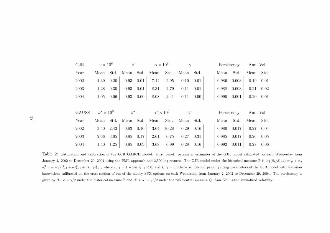
Table 2: Estimation and calibration of the GJR GARCH model. First panel: parameter estimates of the GJR model estimated on each Wednesday from

January 2, 2002 to December 29, 2004 using the PML approach and 3,500 log-returns. The GJR model under the historical measure P is log(St/St−1) = µ + εt,

σ2t = ω + βσ2

t−1 + αε2t−1 + γIt−1ε

2t−1, where It−1 = 1 when εt−1 < 0, and It−1 = 0 otherwise. Second panel: pricing parameters of the GJR model with Gaussian

innovations calibrated on the cross-section of out-of-the-money SPX options on each Wednesday from January 2, 2002 to December 29, 2004. The persistency is

given by β + α + γ/2 under the historical measure P and β∗ + α∗ + γ∗/2 under the risk neutral measure Q. Ann. Vol. is the annualized volatility.

37

FHS ω∗ × 106 β∗ α∗ × 103 γ∗ Persistency Ann. Vol.

Year Mean Std. Mean Std. Mean Std. Mean Std. Mean Std. Mean Std.

2002 3.56 2.98 0.86 0.09 1.62 6.65 0.21 0.14 0.97 0.02 0.21 0.02

2003 3.42 4.91 0.85 0.20 2.17 7.25 0.25 0.36 0.97 0.03 0.21 0.03

2004 1.80 2.03 0.85 0.13 2.39 7.34 0.26 0.22 0.98 0.02 0.19 0.02

HN ω∗hn × 1012 β∗hn α∗

hn × 106 γ∗hn Persistency Ann. Vol.

Year Mean Std. Mean Std. Mean Std. Mean Std. Mean Std. Mean Std.

2002 0.02 0.15 0.53 0.23 4.99 3.33 315.74 60.08 0.96 0.03 0.23 0.03

2003 0.05 0.23 0.66 0.15 2.94 1.94 355.37 83.76 0.98 0.02 0.22 0.03

2004 0.08 0.52 0.42 0.22 2.20 1.71 597.84 206.58 0.97 0.02 0.19 0.02

IG w∗ × 106 b∗ a∗ × 10−3 c∗ × 106 η∗ × 103 Persistency Ann. Vol.

Year Mean Std. Mean Std. Mean Std. Mean Std. Mean Std. Mean Std. Mean Std.

2002 0.14 0.47 0.14 0.20 15.82 14.54 10.77 8.25 −3.88 1.51 0.98 0.02 0.22 0.05

2003 0.08 0.27 0.17 0.22 23.90 16.79 6.64 2.89 −3.33 1.17 0.99 0.00 0.22 0.03

2004 0.04 0.10 0.09 0.14 26.29 14.65 5.18 1.64 −2.65 0.44 0.99 0.00 0.18 0.02

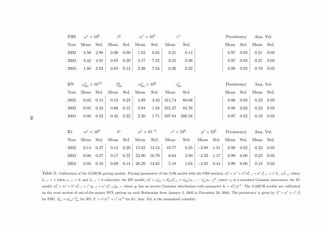
Table 3: Calibration of the GARCH pricing models. Pricing parameters of the GJR model with the FHS method, σ2t = ω∗ + β∗σ2

t−1 + α∗ε2t−1 + γ∗It−1ε

2t−1, where

It−1 = 1 when εt−1 < 0, and It−1 = 0 otherwise; the HN model, σ2t = ω∗

hn + β∗hnσ2

t−1 + α∗hn(zt−1 − γ∗

hnσt−1)2, where zt is a standard Gaussian innovation; the IG

model, σ2t = w∗ + b∗ σ2

t−1 + c∗ yt−1 + a∗ σ4t−1/yt−1, where yt has an inverse Gaussian distribution with parameter δt = σ2

t /η∗2. The GARCH models are calibrated

on the cross section of out-of-the-money SPX options on each Wednesday from January 2, 2002 to December 29, 2004. The persistency is given by β∗ + α∗ + γ∗/2

for FHS, β∗hn + α∗

hnγ∗2

hn for HN, b∗ + a∗η∗2 + c∗/η∗2 for IG, Ann. Vol. is the annualized volatility.

38

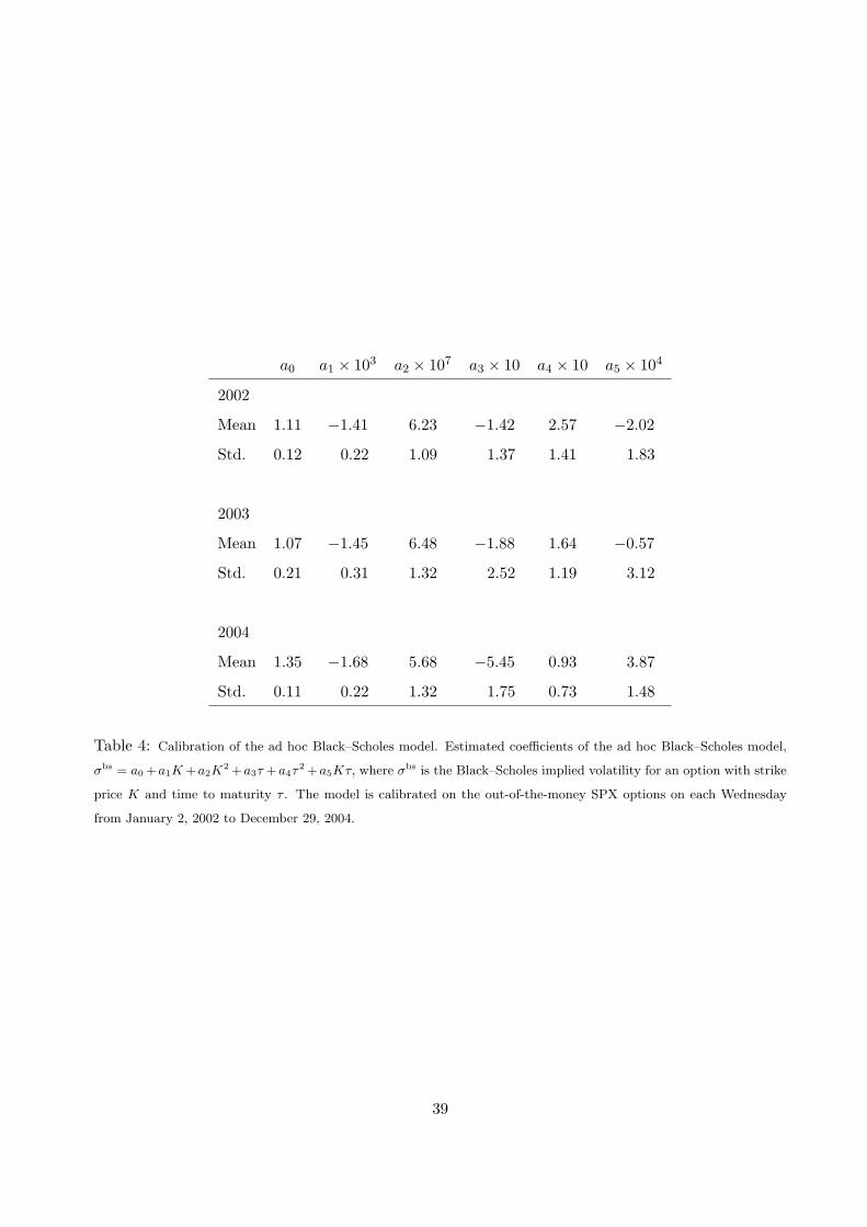
a0 a1 × 103 a2 × 107 a3 × 10 a4 × 10 a5 × 104

2002

Mean 1.11 −1.41 6.23 −1.42 2.57 −2.02

Std. 0.12 0.22 1.09 1.37 1.41 1.83

2003

Mean 1.07 −1.45 6.48 −1.88 1.64 −0.57

Std. 0.21 0.31 1.32 2.52 1.19 3.12

2004

Mean 1.35 −1.68 5.68 −5.45 0.93 3.87

Std. 0.11 0.22 1.32 1.75 0.73 1.48

Table 4: Calibration of the ad hoc Black–Scholes model. Estimated coefficients of the ad hoc Black–Scholes model,

σbs = a0 +a1K +a2K2 +a3τ +a4τ

2 +a5Kτ, where σbs is the Black–Scholes implied volatility for an option with strike

price K and time to maturity τ . The model is calibrated on the out-of-the-money SPX options on each Wednesday

from January 2, 2002 to December 29, 2004.

39

Panel A: Aggregate valuation errors across all years

RMSE MAE MOE Min Max Err>0% ErrBD% MAE% MOE%

FHS 0.87 0.44 0.08 −6.02 4.64 50.50 23.69 21.16 10.75

HN 1.19 0.74 −0.20 −5.66 6.47 30.65 −44.20 23.93 −25.74

IG 1.27 0.77 −0.10 −5.41 6.34 32.06 −32.31 22.49 −25.82

BS 3.39 2.15 0.06 −15.88 28.66 50.82 69.95 57.91 39.46

Panel B: Valuation errors by years

RMSE MAE MOE Min Max Err>0% ErrBD% MAE% MOE%

2002

FHS 0.88 0.43 0.06 −5.63 4.64 47.57 14.67 14.80 4.82

HN 1.16 0.72 −0.21 −4.64 5.55 27.59 −48.00 19.55 −33.06

IG 1.26 0.76 −0.15 −5.14 5.89 27.45 −44.15 19.33 −33.87

BS 3.69 2.36 0.03 −15.25 28.66 48.38 51.20 58.95 39.79

2003

FHS 0.93 0.47 −0.06 −6.02 3.68 44.63 0.95 20.90 6.44

HN 0.92 0.57 −0.28 −3.82 4.92 25.73 −64.94 22.10 −32.13

IG 0.93 0.56 −0.19 −3.72 6.09 27.75 −49.26 20.67 −32.09

BS 3.32 2.12 0.03 −15.88 15.35 49.86 68.37 58.59 38.69

2004

FHS 0.79 0.43 0.23 −3.41 3.90 58.86 53.82 27.61 20.58

HN 1.41 0.91 −0.12 −5.66 6.47 38.24 −21.06 29.92 −12.60

IG 1.53 0.98 0.02 −5.41 6.34 40.62 −4.86 27.27 −12.08

BS 3.15 1.98 0.12 −13.98 15.18 54.11 89.74 56.26 39.85

Table 5: In-sample pricing errors of the different pricing models. RMSE is the root mean square error of the dollar

pricing error (model price−market price); MAE is the dollar average absolute pricing error outside the bid-ask spread

(MAE% is in relative terms and in percentage); MOE is the dollar average pricing error outside the bid-ask spread

(MOE% is in relative terms and in percentage); Min (Max) is the minimum (maximum) pricing error; Err>0% is the

percentage of positive pricing errors; and ErrBD% is the average of 100×(model price−market price)/(bid-ask spread).

40

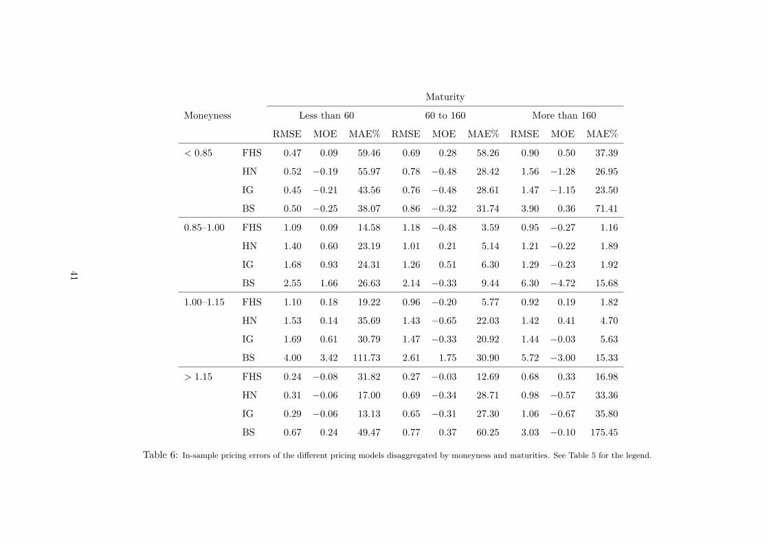
Maturity

Moneyness Less than 60 60 to 160 More than 160

RMSE MOE MAE% RMSE MOE MAE% RMSE MOE MAE%

< 0.85 FHS 0.47 0.09 59.46 0.69 0.28 58.26 0.90 0.50 37.39

HN 0.52 −0.19 55.97 0.78 −0.48 28.42 1.56 −1.28 26.95

IG 0.45 −0.21 43.56 0.76 −0.48 28.61 1.47 −1.15 23.50

BS 0.50 −0.25 38.07 0.86 −0.32 31.74 3.90 0.36 71.41

0.85–1.00 FHS 1.09 0.09 14.58 1.18 −0.48 3.59 0.95 −0.27 1.16

HN 1.40 0.60 23.19 1.01 0.21 5.14 1.21 −0.22 1.89

IG 1.68 0.93 24.31 1.26 0.51 6.30 1.29 −0.23 1.92

BS 2.55 1.66 26.63 2.14 −0.33 9.44 6.30 −4.72 15.68

1.00–1.15 FHS 1.10 0.18 19.22 0.96 −0.20 5.77 0.92 0.19 1.82

HN 1.53 0.14 35.69 1.43 −0.65 22.03 1.42 0.41 4.70

IG 1.69 0.61 30.79 1.47 −0.33 20.92 1.44 −0.03 5.63

BS 4.00 3.42 111.73 2.61 1.75 30.90 5.72 −3.00 15.33

> 1.15 FHS 0.24 −0.08 31.82 0.27 −0.03 12.69 0.68 0.33 16.98

HN 0.31 −0.06 17.00 0.69 −0.34 28.71 0.98 −0.57 33.36

IG 0.29 −0.06 13.13 0.65 −0.31 27.30 1.06 −0.67 35.80

BS 0.67 0.24 49.47 0.77 0.37 60.25 3.03 −0.10 175.45

Table 6: In-sample pricing errors of the different pricing models disaggregated by moneyness and maturities. See Table 5 for the legend.

41

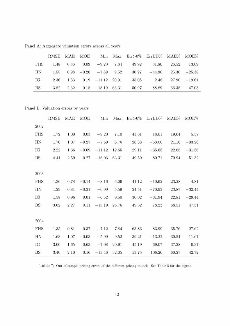
Panel A: Aggregate valuation errors across all years

RMSE MAE MOE Min Max Err>0% ErrBD% MAE% MOE%

FHS 1.48 0.86 0.09 −9.20 7.84 49.92 31.80 26.52 13.09

HN 1.55 0.98 −0.20 −7.69 9.52 30.27 −44.90 25.36 −25.38

IG 2.36 1.33 0.19 −11.12 20.91 35.08 2.48 27.90 −19.61

BS 3.82 2.32 0.18 −18.19 63.31 50.97 88.89 66.38 47.03

Panel B: Valuation errors by years

RMSE MAE MOE Min Max Err>0% ErrBD% MAE% MOE%

2002

FHS 1.72 1.00 0.03 −9.20 7.10 43.61 18.01 19.64 5.57

HN 1.70 1.07 −0.27 −7.69 6.76 26.33 −53.00 21.16 −33.26

IG 2.22 1.36 −0.09 −11.12 12.65 29.11 −35.65 22.68 −31.56

BS 4.41 2.59 0.27 −16.03 63.31 49.59 80.71 70.94 51.32

2003

FHS 1.36 0.78 −0.14 −8.16 6.06 41.12 −10.62 23.28 4.81

HN 1.29 0.81 −0.31 −6.99 5.59 24.51 −70.93 23.87 −32.44

IG 1.58 0.96 0.01 −6.52 9.50 30.02 −31.94 22.81 −29.44

BS 3.62 2.27 0.11 −18.19 26.76 49.32 78.23 68.51 47.51

2004

FHS 1.35 0.81 0.37 −7.12 7.84 63.86 83.99 35.76 27.62

HN 1.63 1.07 −0.03 −5.99 9.52 39.21 −13.22 30.54 −11.67

IG 3.00 1.65 0.63 −7.08 20.91 45.19 69.07 37.38 0.37

BS 3.40 2.10 0.16 −13.46 32.05 53.75 106.26 60.27 42.72

Table 7: Out-of-sample pricing errors of the different pricing models. See Table 5 for the legend.

42

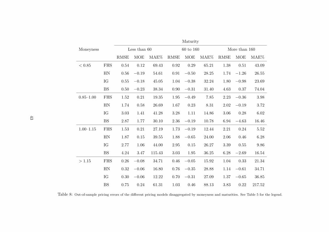
Maturity

Moneyness Less than 60 60 to 160 More than 160

RMSE MOE MAE% RMSE MOE MAE% RMSE MOE MAE%

< 0.85 FHS 0.54 0.12 69.43 0.92 0.29 65.21 1.38 0.51 43.09

HN 0.56 −0.19 54.61 0.91 −0.50 28.25 1.74 −1.26 26.55

IG 0.55 −0.18 45.05 1.04 −0.38 32.24 1.80 −0.98 23.69

BS 0.50 −0.23 38.34 0.90 −0.31 31.40 4.63 0.37 74.04

0.85–1.00 FHS 1.52 0.21 19.35 1.95 −0.49 7.85 2.23 −0.36 3.98

HN 1.74 0.58 26.69 1.67 0.23 8.31 2.02 −0.19 3.72

IG 3.03 1.41 41.28 3.28 1.11 14.86 3.06 0.28 6.02

BS 2.87 1.77 30.10 2.36 −0.19 10.78 6.94 −4.63 16.46

1.00–1.15 FHS 1.53 0.21 27.19 1.73 −0.19 12.44 2.21 0.24 5.52

HN 1.87 0.15 39.55 1.88 −0.65 24.00 2.06 0.46 6.28

IG 2.77 1.06 44.00 2.95 0.15 26.27 3.39 0.55 9.86

BS 4.24 3.47 115.43 3.03 1.95 36.25 6.28 −2.69 16.54

> 1.15 FHS 0.26 −0.08 34.71 0.46 −0.05 15.92 1.04 0.33 21.34

HN 0.32 −0.06 16.80 0.76 −0.35 28.88 1.14 −0.61 34.71

IG 0.30 −0.06 12.22 0.70 −0.31 27.09 1.37 −0.65 36.85

BS 0.75 0.24 61.31 1.03 0.46 88.13 3.83 0.22 217.52

Table 8: Out-of-sample pricing errors of the different pricing models disaggregated by moneyness and maturities. See Table 5 for the legend.

43

Panel A: In-sample aggregate valuation errors across all years

RMSE MAE MOE Min Max Err>0% ErrBD% MAE% MOE%

FHS 0.87 0.44 0.08 −6.02 4.64 50.50 23.69 21.16 10.75

HIST 3.32 1.88 0.22 −19.64 15.29 48.57 35.82 31.38 8.46

GAUSS 0.99 0.53 −0.23 −6.44 4.72 32.38 −18.85 16.72 −2.10

HN 1.19 0.74 −0.20 −5.66 6.47 30.65 −44.20 23.93 −25.74

Panel B: Out-of-sample aggregate valuation errors across all years

RMSE MAE MOE Min Max Err>0% ErrBD% MAE% MOE%

FHS 1.48 0.86 0.09 −9.20 7.84 49.92 31.80 26.52 13.09

HIST 3.33 1.87 0.18 −18.55 16.06 48.56 29.66 31.18 0.31

GAUSS 1.55 0.90 −0.22 −10.13 9.03 37.35 −9.43 22.13 −8.26

HN 1.55 0.98 −0.20 −7.69 9.52 30.27 −44.90 25.36 −25.38

Table 9: In- and out-of-sample pricing errors of the different pricing models. FHS is the GJR GARCH model with FHS

innovations calibrated on the cross-section of out-of-the-money SPX option prices; HIST is the GJR GARCH model

with FHS innovations estimated on historical returns; GAUSS is the GJR GARCH model with Gaussian innovations

calibrated on the cross-section of out-of-the-money SPX option prices; and HN is the Heston–Nandi GARCH model

with Gaussian innovations calibrated on the cross-section of out-of-the-money SPX option prices. See Table 5 for the

legend.

44

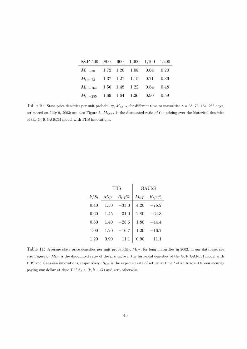
S&P 500 800 900 1,000 1,100 1,200

Mt,t+38 1.72 1.26 1.08 0.64 0.20

Mt,t+73 1.37 1.27 1.15 0.71 0.36

Mt,t+164 1.56 1.48 1.22 0.84 0.48

Mt,t+255 1.69 1.64 1.26 0.90 0.59

Table 10: State price densities per unit probability, Mt,t+τ , for different time to maturities τ = 38, 73, 164, 255 days,

estimated on July 9, 2003; see also Figure 5. Mt,t+τ is the discounted ratio of the pricing over the historical densities

of the GJR GARCH model with FHS innovations.

FHS GAUSS

k/St Mt,T Rt,T % Mt,T Rt,T %

0.40 1.50 −33.3 4.20 −76.2

0.60 1.45 −31.0 2.80 −64.3

0.80 1.40 −28.6 1.80 −44.4

1.00 1.20 −16.7 1.20 −16.7

1.20 0.90 11.1 0.90 11.1

Table 11: Average state price densities per unit probability, Mt,T , for long maturities in 2002, in our database; see

also Figure 6. Mt,T is the discounted ratio of the pricing over the historical densities of the GJR GARCH model with

FHS and Gaussian innovations, respectively. Rt,T is the expected rate of return at time t of an Arrow–Debreu security

paying one dollar at time T if ST ∈ (k, k + dk) and zero otherwise.

45

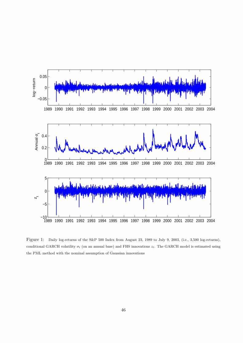
1989 1990 1991 1992 1993 1994 1995 1996 1997 1998 1999 2000 2001 2002 2003 2004

−0.05

0

0.05

log

−re

turn

1989 1990 1991 1992 1993 1994 1995 1996 1997 1998 1999 2000 2001 2002 2003 20040

0.2

0.4

An

nu

al σ

t

1989 1990 1991 1992 1993 1994 1995 1996 1997 1998 1999 2000 2001 2002 2003 2004−10

−5

0

5

z t

Figure 1: Daily log-returns of the S&P 500 Index from August 23, 1989 to July 9, 2003, (i.e., 3,500 log-returns),

conditional GARCH volatility σt (on an annual base) and FHS innovations zt. The GARCH model is estimated using

the PML method with the nominal assumption of Gaussian innovations

46

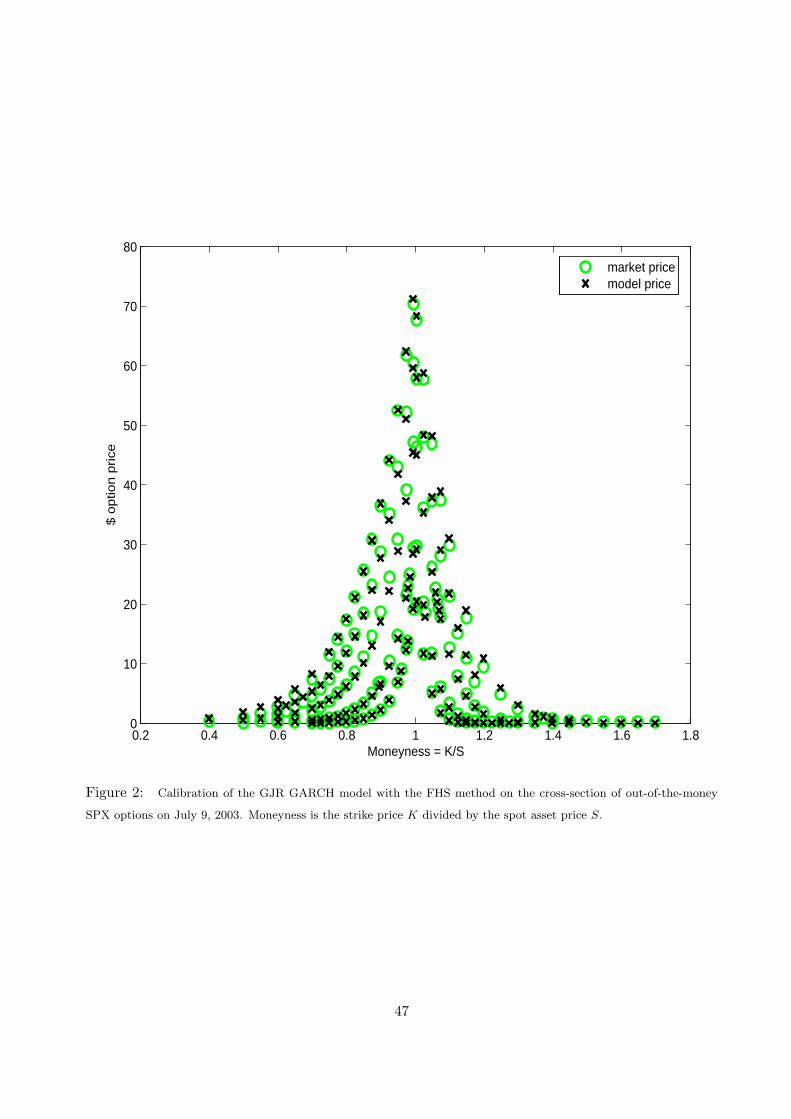
0.2 0.4 0.6 0.8 1 1.2 1.4 1.6 1.80

10

20

30

40

50

60

70

80

Moneyness = K/S

$ o

ptio

n p

rice

market pricemodel price

Figure 2: Calibration of the GJR GARCH model with the FHS method on the cross-section of out-of-the-money

SPX options on July 9, 2003. Moneyness is the strike price K divided by the spot asset price S.

47

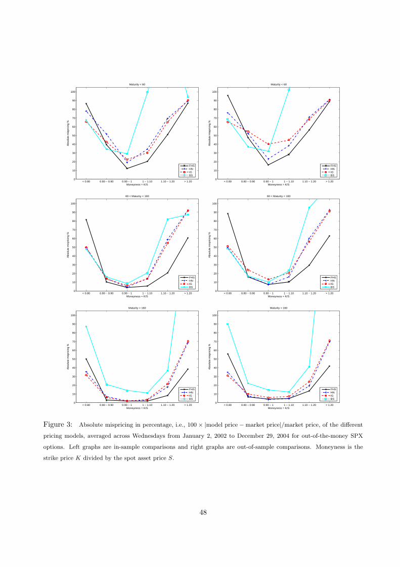
< 0.80 0.80 − 0.90 0.90 − 1 1 − 1.10 1.10 − 1.20 > 1.200

10

20

30

40

50

60

70

80

90

100

Moneyness = K/S

Abs

olut

e m

ispr

icin

g %

Maturity < 60

FHSHNIGBS

< 0.80 0.80 − 0.90 0.90 − 1 1 − 1.10 1.10 − 1.20 > 1.200

10

20

30

40

50

60

70

80

90

100

Moneyness = K/S

Abs

olut

e m

ispr

icin

g %

Maturity < 60

FHSHNIGBS

< 0.80 0.80 − 0.90 0.90 − 1 1 − 1.10 1.10 − 1.20 > 1.200

10

20

30

40

50

60

70

80

90

100

Moneyness = K/S

Abs

olut

e m

ispr

icin

g %

60 < Maturity < 160

FHSHNIGBS

< 0.80 0.80 − 0.90 0.90 − 1 1 − 1.10 1.10 − 1.20 > 1.200

10

20

30

40

50

60

70

80

90

100

Moneyness = K/S

Abs

olut

e m

ispr

icin

g %

60 < Maturity < 160

FHSHNIGBS

< 0.80 0.80 − 0.90 0.90 − 1 1 − 1.10 1.10 − 1.20 > 1.200

10

20

30

40

50

60

70

80

90

100

Moneyness = K/S

Abs

olut

e m

ispr

icin

g %

Maturity > 160

FHSHNIGBS

< 0.80 0.80 − 0.90 0.90 − 1 1 − 1.10 1.10 − 1.20 > 1.200

10

20

30

40

50

60

70

80

90

100

Moneyness = K/S

Abs

olut

e m

ispr

icin

g %

Maturity > 160

FHSHNIGBS

Figure 3: Absolute mispricing in percentage, i.e., 100 × |model price − market price|/market price, of the different

pricing models, averaged across Wednesdays from January 2, 2002 to December 29, 2004 for out-of-the-money SPX

options. Left graphs are in-sample comparisons and right graphs are out-of-sample comparisons. Moneyness is the

strike price K divided by the spot asset price S.

48

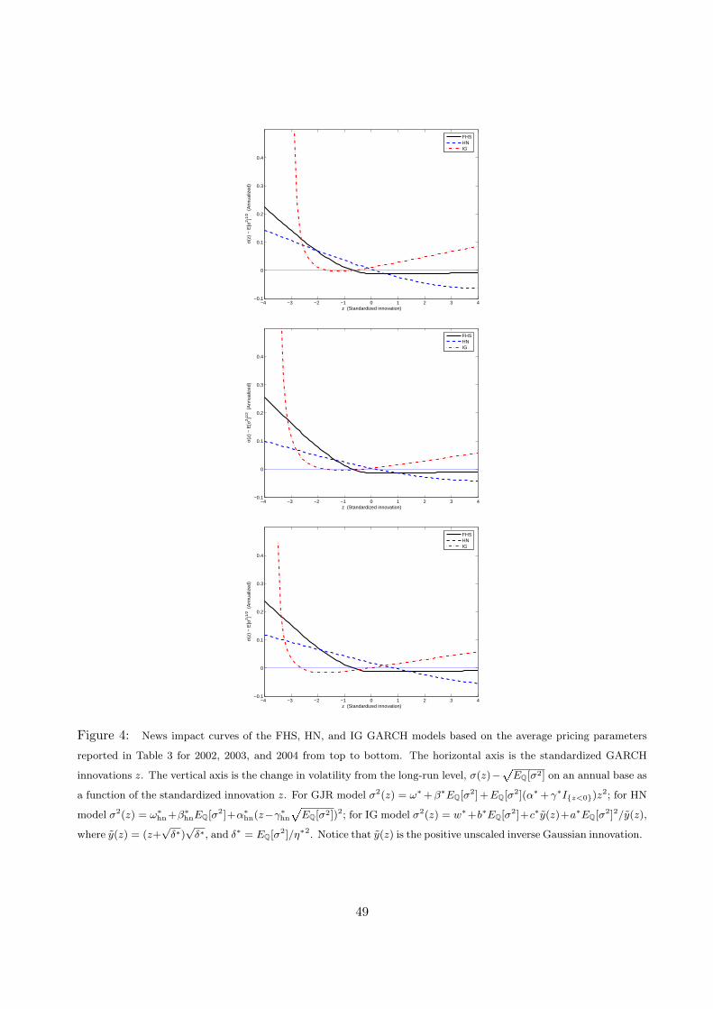
−4 −3 −2 −1 0 1 2 3 4−0.1

0

0.1

0.2

0.3

0.4

z (Standardized innovation)

σ(z)

− E

[σ2 ]1/

2 (A

nnua

lized

)

FHSHNIG

−4 −3 −2 −1 0 1 2 3 4−0.1

0

0.1

0.2

0.3

0.4

z (Standardized innovation)

σ(z)

− E

[σ2 ]1/

2 (A

nnua

lized

)

FHSHNIG

−4 −3 −2 −1 0 1 2 3 4−0.1

0

0.1

0.2

0.3

0.4

z (Standardized innovation)

σ(z)

− E

[σ2 ]1/

2 (A

nnua

lized

)

FHSHNIG

Figure 4: News impact curves of the FHS, HN, and IG GARCH models based on the average pricing parameters

reported in Table 3 for 2002, 2003, and 2004 from top to bottom. The horizontal axis is the standardized GARCH

innovations z. The vertical axis is the change in volatility from the long-run level, σ(z)−p

EQ[σ2] on an annual base as

a function of the standardized innovation z. For GJR model σ2(z) = ω∗ +β∗EQ[σ2]+EQ[σ2](α∗ +γ∗I{z<0})z2; for HN

model σ2(z) = ω∗hn+β∗

hnEQ[σ2]+α∗hn(z−γ∗

hn

pEQ[σ2])2; for IG model σ2(z) = w∗+b∗EQ[σ2]+c∗y(z)+a∗EQ[σ2]2/y(z),

where y(z) = (z+√

δ∗)√

δ∗, and δ∗ = EQ[σ2]/η∗2. Notice that y(z) is the positive unscaled inverse Gaussian innovation.

49

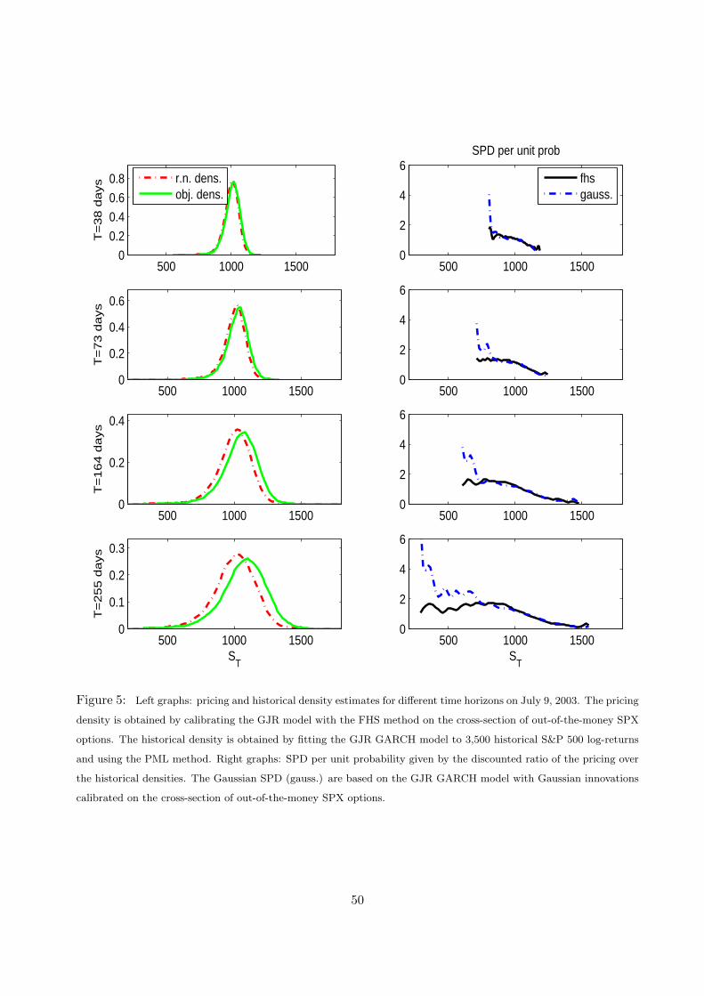
500 1000 15000

0.2

0.4

0.6

0.8

T=

38

da

ys

500 1000 15000

2

4

6SPD per unit prob

500 1000 15000

0.2

0.4

0.6

T=

73

da

ys

500 1000 15000

2

4

6

500 1000 15000

0.2

0.4

T=

16

4 d

ays

500 1000 15000

2

4

6

500 1000 15000

0.1

0.2

0.3

T=

25

5 d

ays

ST

500 1000 15000

2

4

6

ST

r.n. dens.obj. dens.

fhsgauss.

Figure 5: Left graphs: pricing and historical density estimates for different time horizons on July 9, 2003. The pricing

density is obtained by calibrating the GJR model with the FHS method on the cross-section of out-of-the-money SPX

options. The historical density is obtained by fitting the GJR GARCH model to 3,500 historical S&P 500 log-returns

and using the PML method. Right graphs: SPD per unit probability given by the discounted ratio of the pricing over

the historical densities. The Gaussian SPD (gauss.) are based on the GJR GARCH model with Gaussian innovations

calibrated on the cross-section of out-of-the-money SPX options.

50

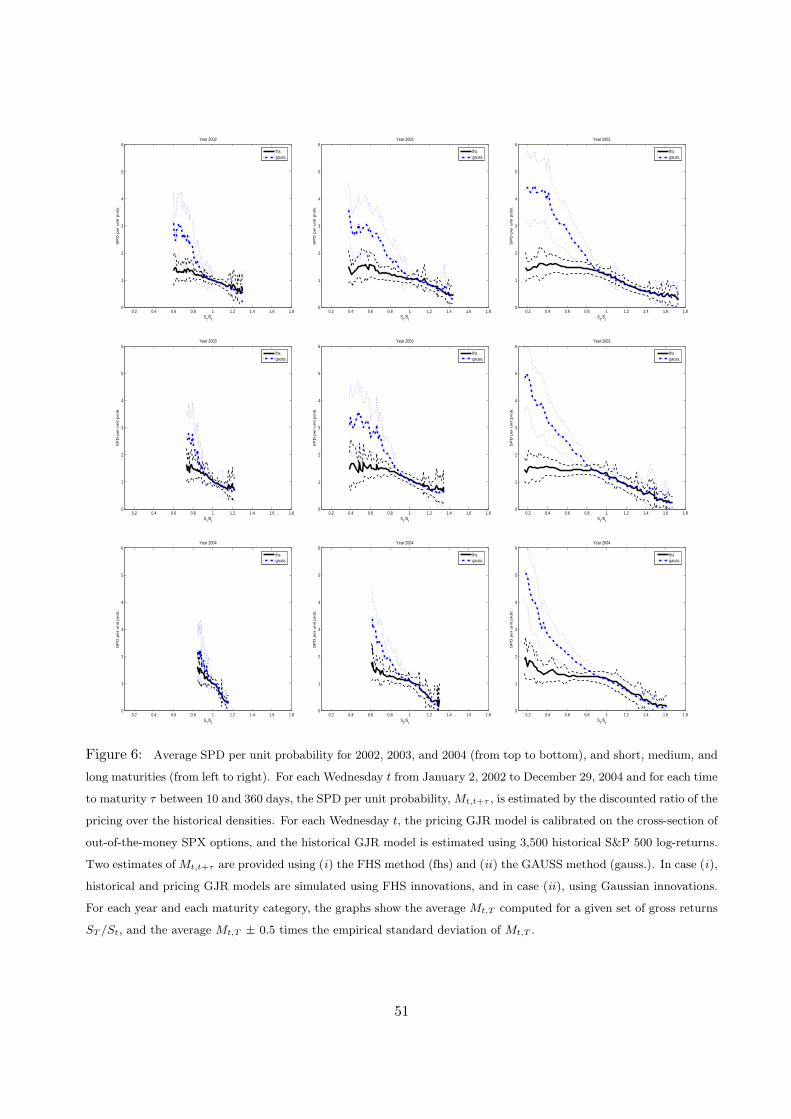
0.2 0.4 0.6 0.8 1 1.2 1.4 1.6 1.80

1

2

3

4

5

6

ST/S

t

SP

D p

er

un

it p

rob

.

Year 2002

fhsgauss.

0.2 0.4 0.6 0.8 1 1.2 1.4 1.6 1.80

1

2

3

4

5

6

ST/S

t

SP

D p

er

un

it p

rob

.

Year 2002

fhsgauss.

0.2 0.4 0.6 0.8 1 1.2 1.4 1.6 1.80

1

2

3

4

5

6

ST/S

t

SP

D p

er

un

it p

rob

.

Year 2002

fhsgauss.

0.2 0.4 0.6 0.8 1 1.2 1.4 1.6 1.80

1

2

3

4

5

6

ST/S

t

SP

D p

er

un

it p

rob

.

Year 2003

fhsgauss.

0.2 0.4 0.6 0.8 1 1.2 1.4 1.6 1.80

1

2

3

4

5

6

ST/S

t

SP

D p

er

un

it p

rob

.

Year 2003

fhsgauss.

0.2 0.4 0.6 0.8 1 1.2 1.4 1.6 1.80

1

2

3

4

5

6

ST/S

t

SP

D p

er

un

it p

rob

.

Year 2003

fhsgauss.

0.2 0.4 0.6 0.8 1 1.2 1.4 1.6 1.80

1

2

3

4

5

6

ST/S

t

SP

D p

er

un

it p

rob

.

Year 2004

fhsgauss.

0.2 0.4 0.6 0.8 1 1.2 1.4 1.6 1.80

1

2

3

4

5

6

ST/S

t

SP

D p

er

un

it p

rob

.

Year 2004

fhsgauss.

0.2 0.4 0.6 0.8 1 1.2 1.4 1.6 1.80

1

2

3

4

5

6

ST/S

t

SP

D p

er

un

it p

rob

.

Year 2004

fhsgauss.

Figure 6: Average SPD per unit probability for 2002, 2003, and 2004 (from top to bottom), and short, medium, and

long maturities (from left to right). For each Wednesday t from January 2, 2002 to December 29, 2004 and for each time

to maturity τ between 10 and 360 days, the SPD per unit probability, Mt,t+τ , is estimated by the discounted ratio of the

pricing over the historical densities. For each Wednesday t, the pricing GJR model is calibrated on the cross-section of

out-of-the-money SPX options, and the historical GJR model is estimated using 3,500 historical S&P 500 log-returns.

Two estimates of Mt,t+τ are provided using (i) the FHS method (fhs) and (ii) the GAUSS method (gauss.). In case (i),

historical and pricing GJR models are simulated using FHS innovations, and in case (ii), using Gaussian innovations.

For each year and each maturity category, the graphs show the average Mt,T computed for a given set of gross returns

ST /St, and the average Mt,T ± 0.5 times the empirical standard deviation of Mt,T .

51

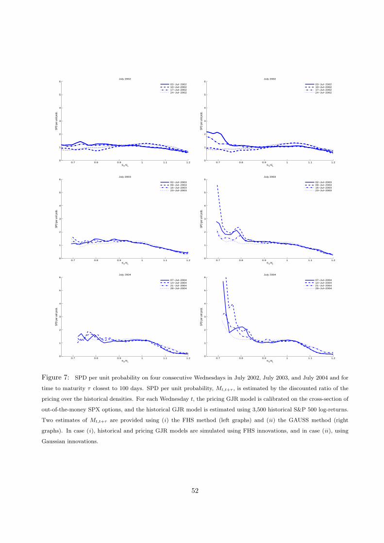
0.7 0.8 0.9 1 1.1 1.20

1

2

3

4

5

6

ST/S

t

SPD

per u

nit p

rob.

July 2002

03−Jul−200210−Jul−200217−Jul−200224−Jul−2002

0.7 0.8 0.9 1 1.1 1.20

1

2

3

4

5

6

ST/S

t

SPD

per u

nit p

rob.

July 2002

03−Jul−200210−Jul−200217−Jul−200224−Jul−2002

0.7 0.8 0.9 1 1.1 1.20

1

2

3

4

5

6

ST/S

t

SPD

per u

nit p

rob.

July 2003

02−Jul−200309−Jul−200316−Jul−200323−Jul−2003

0.7 0.8 0.9 1 1.1 1.20

1

2

3

4

5

6

ST/S

t

SPD

per u

nit p

rob.

July 2003

02−Jul−200309−Jul−200316−Jul−200323−Jul−2003

0.7 0.8 0.9 1 1.1 1.20

1

2

3

4

5

6

ST/S

t

SPD

per u

nit p

rob.

July 2004

07−Jul−200414−Jul−200421−Jul−200428−Jul−2004

0.7 0.8 0.9 1 1.1 1.20

1

2

3

4

5

6

ST/S

t

SPD

per u

nit p

rob.

July 2004

07−Jul−200414−Jul−200421−Jul−200428−Jul−2004

Figure 7: SPD per unit probability on four consecutive Wednesdays in July 2002, July 2003, and July 2004 and for

time to maturity τ closest to 100 days. SPD per unit probability, Mt,t+τ , is estimated by the discounted ratio of the

pricing over the historical densities. For each Wednesday t, the pricing GJR model is calibrated on the cross-section of

out-of-the-money SPX options, and the historical GJR model is estimated using 3,500 historical S&P 500 log-returns.

Two estimates of Mt,t+τ are provided using (i) the FHS method (left graphs) and (ii) the GAUSS method (right

graphs). In case (i), historical and pricing GJR models are simulated using FHS innovations, and in case (ii), using

Gaussian innovations.

52

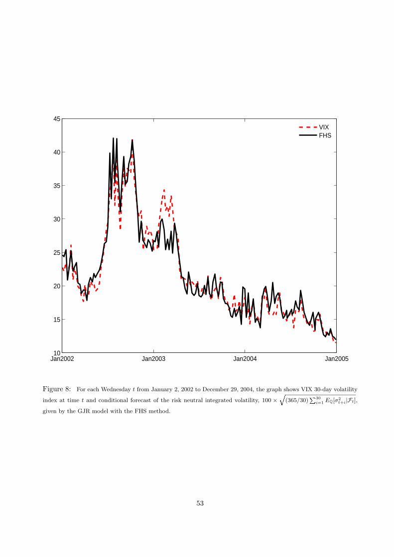
Jan2002 Jan2003 Jan2004 Jan200510

15

20

25

30

35

40

45

VIXFHS

Figure 8: For each Wednesday t from January 2, 2002 to December 29, 2004, the graph shows VIX 30-day volatility

index at time t and conditional forecast of the risk neutral integrated volatility, 100 ×q

(365/30)P30

i=1EQ[σ2

t+i|Ft],

given by the GJR model with the FHS method.

53