Embed Size (px)
Citation preview
A Further Examination of Insurance Pricing And
Underwriting Cycles
July, 2005
Madsen, Chris K. GE Insurance Solutions
Østbanegade 135, 2100 Copenhagen Ø, Denmark Phone: +45 33 97 95 02, Fax: +45 33 97 94 41
E-Mail: [email protected]
Haastrup, Svend GE Insurance Solutions
Østbanegade 135, 2100 Copenhagen Ø, Denmark Phone: +45 33 18 95 75, Fax: +45 33 97 94 41
E-Mail: [email protected]
Pedersen, Hal W. Warren Centre for Actuarial Studies and Research
Faculty of Management University of Manitoba
Winnipeg, Manitoba R3X 1J8, Canada Phone: +1 204 474 9529
E-Mail: [email protected]
Abstract This paper is a follow-up to the paper “An Examination of Insurance Pricing and Underwriting Cycles”. In that paper, Madsen and Pedersen laid out a theory of a "price of risk" and suggested that this price links all risky financial transactions. In particular, the paper detailed insurance pricing in terms of this price of risk and supported this with an analysis of the performance of the property and casualty insurance industry for the past fifty years. In this paper, we follow up on some of the questions raised as feedback to the original paper. In addition, we offer some more specific examples based on actual treaty data. We also extend the use of this to a broader framework and put forth a plausible explanation for why our industry has been relatively slow to develop a complete and coherent pricing theory. We discuss that the lack of a coherent pricing theory may in fact be amplifying the underwriting cycle due to consistent mis-pricing. We recognize that some of our hypotheses are controversial, but we believe a healthy debate – supported with actual data and underlying pricing theory - is necessary to move our industry and its theory of price forward. Key Words Price of risk, risk-adjusted value of insurance, insurance pricing, option pricing, underwriting cycle, property and casualty insurance, general insurance, market cycle, implied volatility
2
Table of Contents Introduction......................................................................................................................... 4 Background and Review..................................................................................................... 4 What is Insurance?.............................................................................................................. 6 Pricing Framework............................................................................................................ 13 Two Real-Case Examples ................................................................................................. 14
The Industry Combined Ratio and General Profitability.............................................. 14 Reviewing Actual Data from a Low-volatility Line of Business ................................. 16
Hypothesis............................................................................................................. 20 Test........................................................................................................................ 20
Why? ................................................................................................................................. 25 Summary and Conclusion ................................................................................................. 27 Appendix........................................................................................................................... 28
The Expected Payoff of a Reinsurance Contract Given an Underlying Log-Normal Distribution ................................................................................................................... 28
First Moment..................................................................................................... 28 Second Moment ................................................................................................ 28
References......................................................................................................................... 29
3
Introduction Insurance needs a coherent pricing theory. Current actuarial pricing does not account for the optionality offered by insurance contracts. It is loss estimation rather than pricing and will only generate acceptable results under elusive conditions. Promoting a common understanding of the difference between these two terms is essential in moving our industry forward. The views expressed in this paper are those of the authors. We know they are controversial, but we believe that a healthy debate is necessary to accelerate the development of a coherent pricing theory in insurance. This paper is a follow-up to the paper by Madsen and Pedersen, 2003. In this paper, we follow up with some more concrete examples and explore further some of the feedback we have received in the past two years. Some of the questions that continually haunt the property casualty industry include the following:
Why are property casualty insurers’ returns on equity continually so dismal? Why do property casualty insurers keep entertaining so many perspectives on risk
management and pricing? Why do property casualty insurers have so many actuaries? Why do many property casualty insurers think their business is more art than
science? Why is the underwriting cycle such a mystery and why is it so amplified?
We suggest that the answer to these questions is, at least in part, the lack of a coherent pricing theory.
Background and Review As suggested in “An Examination of Insurance Pricing”, selling insurance is like selling call options. We suggested then that the underwriting cycle was a direct result of insurers lack of pricing for the inherent optionality in insurance portfolios. Insurance is ripe with options. Consider the following:
Simple Example An insurer, A Insurance, buys reinsurance from a reinsurer, B Re. It is a stop-loss treaty covering property claims arising during the next year. At the moment of underwriting, B Re does not know the amount of premium that A Insurance will
4
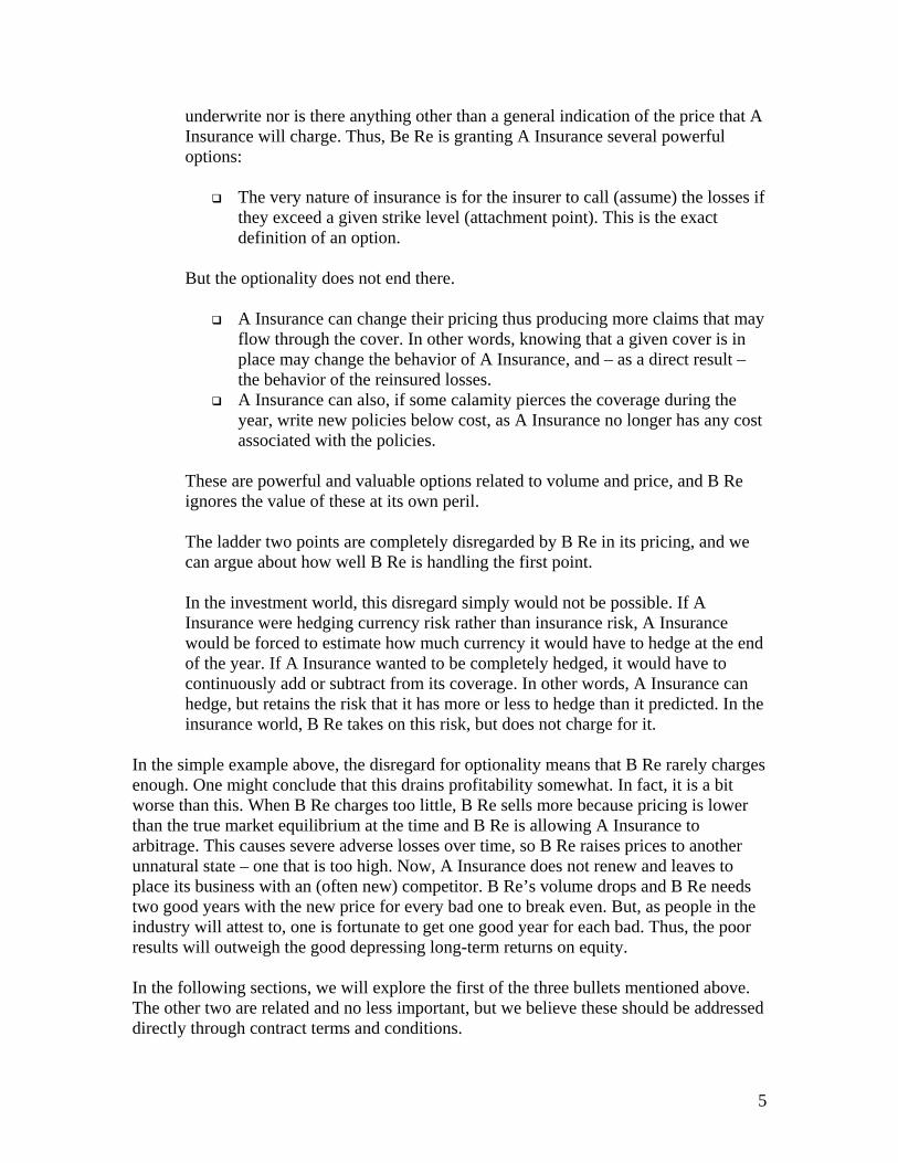
underwrite nor is there anything other than a general indication of the price that A Insurance will charge. Thus, Be Re is granting A Insurance several powerful options:
The very nature of insurance is for the insurer to call (assume) the losses if they exceed a given strike level (attachment point). This is the exact definition of an option.
But the optionality does not end there.
A Insurance can change their pricing thus producing more claims that may flow through the cover. In other words, knowing that a given cover is in place may change the behavior of A Insurance, and – as a direct result – the behavior of the reinsured losses.
A Insurance can also, if some calamity pierces the coverage during the year, write new policies below cost, as A Insurance no longer has any cost associated with the policies.
These are powerful and valuable options related to volume and price, and B Re ignores the value of these at its own peril. The ladder two points are completely disregarded by B Re in its pricing, and we can argue about how well B Re is handling the first point. In the investment world, this disregard simply would not be possible. If A Insurance were hedging currency risk rather than insurance risk, A Insurance would be forced to estimate how much currency it would have to hedge at the end of the year. If A Insurance wanted to be completely hedged, it would have to continuously add or subtract from its coverage. In other words, A Insurance can hedge, but retains the risk that it has more or less to hedge than it predicted. In the insurance world, B Re takes on this risk, but does not charge for it.
In the simple example above, the disregard for optionality means that B Re rarely charges enough. One might conclude that this drains profitability somewhat. In fact, it is a bit worse than this. When B Re charges too little, B Re sells more because pricing is lower than the true market equilibrium at the time and B Re is allowing A Insurance to arbitrage. This causes severe adverse losses over time, so B Re raises prices to another unnatural state – one that is too high. Now, A Insurance does not renew and leaves to place its business with an (often new) competitor. B Re’s volume drops and B Re needs two good years with the new price for every bad one to break even. But, as people in the industry will attest to, one is fortunate to get one good year for each bad. Thus, the poor results will outweigh the good depressing long-term returns on equity. In the following sections, we will explore the first of the three bullets mentioned above. The other two are related and no less important, but we believe these should be addressed directly through contract terms and conditions.
5
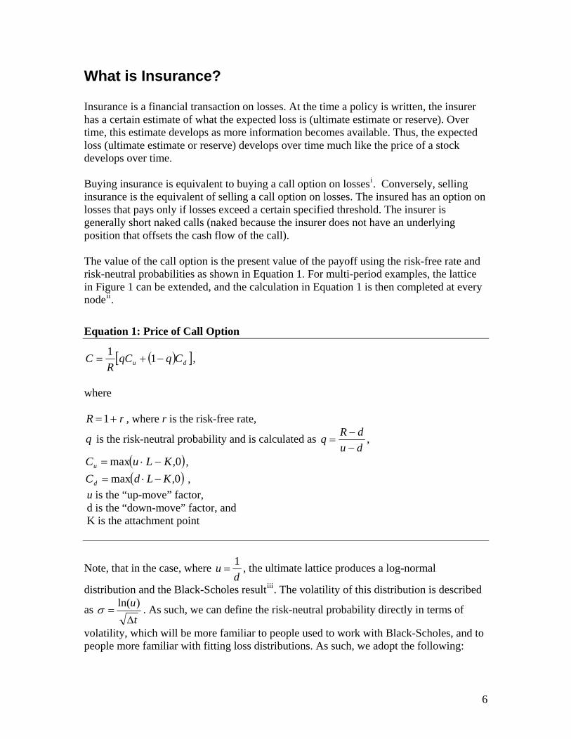
What is Insurance? Insurance is a financial transaction on losses. At the time a policy is written, the insurer has a certain estimate of what the expected loss is (ultimate estimate or reserve). Over time, this estimate develops as more information becomes available. Thus, the expected loss (ultimate estimate or reserve) develops over time much like the price of a stock develops over time. Buying insurance is equivalent to buying a call option on lossesi. Conversely, selling insurance is the equivalent of selling a call option on losses. The insured has an option on losses that pays only if losses exceed a certain specified threshold. The insurer is generally short naked calls (naked because the insurer does not have an underlying position that offsets the cash flow of the call). The value of the call option is the present value of the payoff using the risk-free rate and risk-neutral probabilities as shown in Equation 1. For multi-period examples, the lattice in Figure 1 can be extended, and the calculation in Equation 1 is then completed at every nodeii.
Equation 1: Price of Call Option
( )[ ]du CqqCR
C −+= 11 ,
where
rR +=1 , where r is the risk-free rate,
q is the risk-neutral probability and is calculated as dudRq
−−
= ,
( )0,max KLuCu −⋅= , ( )0,max KLdCd −⋅= ,
u is the “up-move” factor, d is the “down-move” factor, and K is the attachment point
Note, that in the case, where d
u 1= , the ultimate lattice produces a log-normal
distribution and the Black-Scholes resultiii. The volatility of this distribution is described
as t
uΔ
=)ln(σ . As such, we can define the risk-neutral probability directly in terms of
volatility, which will be more familiar to people used to work with Black-Scholes, and to people more familiar with fitting loss distributions. As such, we adopt the following:
6
teu Δ= σ ted Δ−= σ
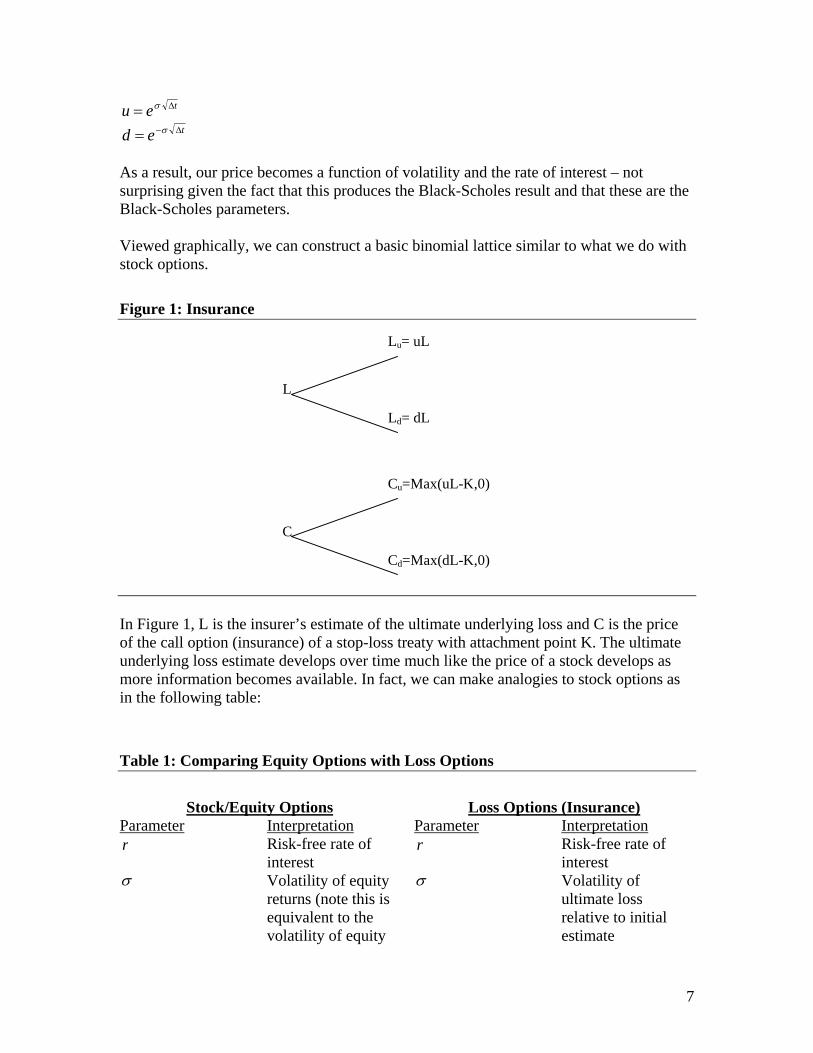
As a result, our price becomes a function of volatility and the rate of interest – not surprising given the fact that this produces the Black-Scholes result and that these are the Black-Scholes parameters. Viewed graphically, we can construct a basic binomial lattice similar to what we do with stock options.
Figure 1: Insurance
Ld= dL
L
Lu= uL
Cd=Max(dL-K,0)
C
Cu=Max(uL-K,0)
In Figure 1, L is the insurer’s estimate of the ultimate underlying loss and C is the price of the call option (insurance) of a stop-loss treaty with attachment point K. The ultimate underlying loss estimate develops over time much like the price of a stock develops as more information becomes available. In fact, we can make analogies to stock options as in the following table:
Table 1: Comparing Equity Options with Loss Options
Stock/Equity Options Loss Options (Insurance)
Parameter Interpretation Parameter Interpretation Risk-free rate of
interest r r Risk-free rate of
interest σ Volatility of equity
returns (note this is equivalent to the volatility of equity
σ Volatility of ultimate loss relative to initial estimate
7
prices divided by the beginning equity price)
0S Equity price at time 0
0L Discounted ultimate loss estimate at time 0
tS Equity price at time t
tL Ultimate loss estimate at time t
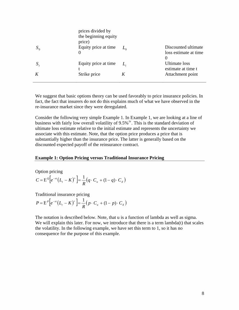
K Strike price K Attachment point We suggest that basic options theory can be used favorably to price insurance policies. In fact, the fact that insurers do not do this explains much of what we have observed in the re-insurance market since they were deregulated. Consider the following very simple Example 1. In Example 1, we are looking at a line of business with fairly low overall volatility of 9.5%iv. This is the standard deviation of ultimate loss estimate relative to the initial estimate and represents the uncertainty we associate with this estimate. Note, that the option price produces a price that is substantially higher than the insurance price. The latter is generally based on the discounted expected payoff of the reinsurance contract.
Example 1: Option Pricing versus Traditional Insurance Pricing
Option pricing
( )[ ] ( )dutrtQ CqCq
RKLeC ⋅−+⋅=−Ε= +− )1(1
Traditional insurance pricing
( )[ ] ( )dutrtP CpCp
RKLeP ⋅−+⋅=−Ε= +− )1(1
The notation is described below. Note, that u is a function of lambda as well as sigma. We will explain this later. For now, we introduce that there is a term lambda(t) that scales the volatility. In the following example, we have set this term to 1, so it has no consequence for the purpose of this example.
8
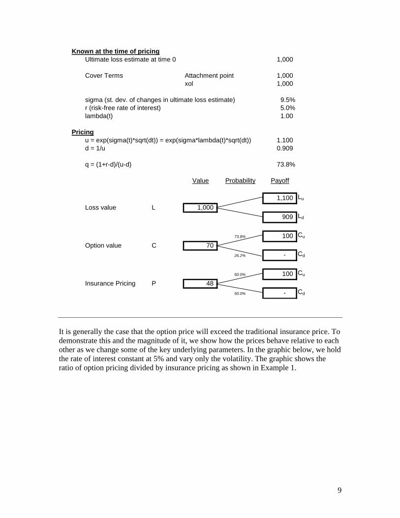
Known at the time of pricingUltimate loss estimate at time 0 1,000
Cover Terms Attachment point 1,000 xol 1,000
sigma (st. dev. of changes in ultimate loss estimate) 9.5%r (risk-free rate of interest) 5.0%lambda(t) 1.00
Pricingu = exp(sigma(t)*sqrt(dt)) = exp(sigma*lambda(t)*sqrt(dt)) 1.100 d = 1/u 0.909
q = (1+r-d)/(u-d) 73.8%
Value Probability Payoff
1,100 Lu
Loss value L 1,000 909 Ld
73.8% 100 Cu
Option value C 70 26.2% - Cd
50.0% 100 Cu
Insurance Pricing P 48 50.0% - Cd
It is generally the case that the option price will exceed the traditional insurance price. To demonstrate this and the magnitude of it, we show how the prices behave relative to each other as we change some of the key underlying parameters. In the graphic below, we hold the rate of interest constant at 5% and vary only the volatility. The graphic shows the ratio of option pricing divided by insurance pricing as shown in Example 1.
9
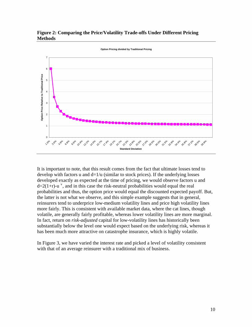
Figure 2: Comparing the Price/Volatility Trade-offs Under Different Pricing Methods
Option Pricing divided by Traditional Pricing
0
1
2
3
4
5
6
7
1.0%
3.0%
4.9%
6.8%
8.6%
10.4%
12.2%
14.0%
15.7%
17.4%
19.1%
20.7%
22.3%
23.9%
25.5%
27.0%
28.5%
30.0%
31.5%
32.9%
34.4%
35.8%
37.2%
38.5%
39.9%
Standard Deviation
Opt
ion
Pric
e R
elat
ive
to T
radi
tiona
l Pric
e
It is important to note, that this result comes from the fact that ultimate losses tend to develop with factors u and d=1/u (similar to stock prices). If the underlying losses developed exactly as expected at the time of pricing, we would observe factors u and d=2(1+r)-u v, and in this case the risk-neutral probabilities would equal the real probabilities and thus, the option price would equal the discounted expected payoff. But, the latter is not what we observe, and this simple example suggests that in general, reinsurers tend to underprice low-medium volatility lines and price high volatility lines more fairly. This is consistent with available market data, where the cat lines, though volatile, are generally fairly profitable, whereas lower volatility lines are more marginal. In fact, return on risk-adjusted capital for low-volatility lines has historically been substantially below the level one would expect based on the underlying risk, whereas it has been much more attractive on catastrophe insurance, which is highly volatile. In Figure 3, we have varied the interest rate and picked a level of volatility consistent with that of an average reinsurer with a traditional mix of business.
10
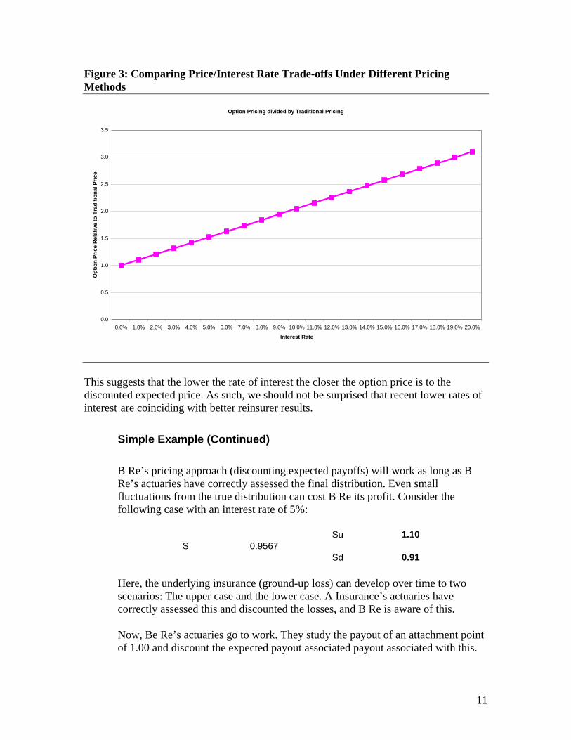
Figure 3: Comparing Price/Interest Rate Trade-offs Under Different Pricing Methods
Option Pricing divided by Traditional Pricing
0.0
0.5
1.0
1.5
2.0
2.5
3.0
3.5
0.0% 1.0% 2.0% 3.0% 4.0% 5.0% 6.0% 7.0% 8.0% 9.0% 10.0% 11.0% 12.0% 13.0% 14.0% 15.0% 16.0% 17.0% 18.0% 19.0% 20.0%
Interest Rate
Opt
ion
Pric
e R
elat
ive
to T
radi
tiona
l Pric
e
This suggests that the lower the rate of interest the closer the option price is to the discounted expected price. As such, we should not be surprised that recent lower rates of interest are coinciding with better reinsurer results.
Simple Example (Continued)
B Re’s pricing approach (discounting expected payoffs) will work as long as B Re’s actuaries have correctly assessed the final distribution. Even small fluctuations from the true distribution can cost B Re its profit. Consider the following case with an interest rate of 5%:
Su 1.10 S 0.9567
Sd 0.91
Here, the underlying insurance (ground-up loss) can develop over time to two scenarios: The upper case and the lower case. A Insurance’s actuaries have correctly assessed this and discounted the losses, and B Re is aware of this. Now, Be Re’s actuaries go to work. They study the payout of an attachment point of 1.00 and discount the expected payout associated payout associated with this.
11
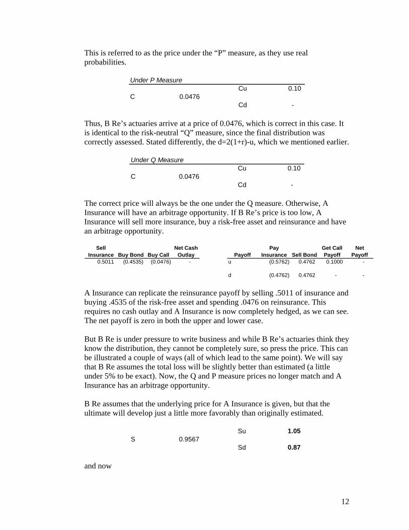
This is referred to as the price under the “P” measure, as they use real probabilities.
Under P MeasureCu 0.10
C 0.0476 Cd -
Thus, B Re’s actuaries arrive at a price of 0.0476, which is correct in this case. It is identical to the risk-neutral “Q” measure, since the final distribution was correctly assessed. Stated differently, the d=2(1+r)-u, which we mentioned earlier.
Under Q MeasureCu 0.10
C 0.0476 Cd -
The correct price will always be the one under the Q measure. Otherwise, A Insurance will have an arbitrage opportunity. If B Re’s price is too low, A Insurance will sell more insurance, buy a risk-free asset and reinsurance and have an arbitrage opportunity.
Sell Insurance Buy Bond Buy Call
Net Cash Outlay Payoff
Pay Insurance Sell Bond
Get Call Payoff
Net Payoff
0.5011 (0.4535) (0.0476) - u (0.5762) 0.4762 0.1000 -
d (0.4762) 0.4762 - - A Insurance can replicate the reinsurance payoff by selling .5011 of insurance and buying .4535 of the risk-free asset and spending .0476 on reinsurance. This requires no cash outlay and A Insurance is now completely hedged, as we can see. The net payoff is zero in both the upper and lower case. But B Re is under pressure to write business and while B Re’s actuaries think they know the distribution, they cannot be completely sure, so press the price. This can be illustrated a couple of ways (all of which lead to the same point). We will say that B Re assumes the total loss will be slightly better than estimated (a little under 5% to be exact). Now, the Q and P measure prices no longer match and A Insurance has an arbitrage opportunity. B Re assumes that the underlying price for A Insurance is given, but that the ultimate will develop just a little more favorably than originally estimated.
Su 1.05 S 0.9567
Sd 0.87 and now
12
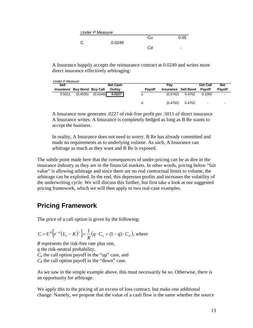
Under P MeasureCu 0.05
C 0.0249 Cd -
A Insurance happily accepts the reinsurance contract at 0.0249 and writes more direct insurance effectively arbitraging: Under P Measure
Sell Insurance Buy Bond Buy Call
Net Cash Outlay Payoff
Pay Insurance Sell Bond
Get Call Payoff
Net Payoff
0.5011 (0.4535) (0.0249) 0.0227 u (0.5762) 0.4762 0.1000 -
d (0.4762) 0.4762 - - A Insurance now generates .0227 of risk-free profit per .5011 of direct insurance A Insurance writes. A Insurance is completely hedged as long as B Re wants to accept the business. In reality, A Insurance does not need to worry. B Re has already committed and made no requirements as to underlying volume. As such, A Insurance can arbitrage as much as they want and B Re is exposed.
The subtle point made here that the consequences of under-pricing can be as dire in the insurance industry as they are in the financial markets. In other words, pricing below “fair value” is allowing arbitrage and since there are no real contractual limits to volume, the arbitrage can be exploited. In the end, this depresses profits and increases the volatility of the underwriting cycle. We will discuss this further, but first take a look at our suggested pricing framework, which we will then apply to two real-case examples.
Pricing Framework The price of a call option is given by the following:
( )[ ] ( )dutrtQ CqCq
RKLeC ⋅−+⋅=−Ε= +− )1(1 , where
R represents the risk-free rate plus one, q the risk-neutral probability, Cu the call option payoff in the “up” case, and Cd the call option payoff in the “down” case. As we saw in the simple example above, this must necessarily be so. Otherwise, there is an opportunity for arbitrage. We apply this to the pricing of an excess of loss contract, but make one additional change. Namely, we propose that the value of a cash flow is the same whether the source
13
is insurance, equities or some other financial asset. In other words, we recognize that there is a single price of risk that permeates all financial transactions. This price of risk can be described by the implied option volatility and we have observable market prices for this through the Chicago Board Options Exchange (CBOE) “Vix”, which trade at the average implied volatility of several S&P 500 options. When the Vix are high, the price of risk is high as the markets perceive greater risk. We submit that this translates to transactions beyond the equity marketsvi.
tt
t
tt
t
tt
t
tt
t
eeeR
eeeR
dudRq
Δ−Δ
Δ−
Δ−Δ
Δ−
−
−=
−
−=
−−
= **
*
σλσλ
σλ
σσ
σ
, where
vixvixt
t =*λ ,
N
vixvix
N
tt∑
== 1 ,
σ is the long-term standard deviation of the underlying ultimate loss estimate divided by the initial loss estimate,
tσ is the standard deviation at time t reflecting the market price of risk (estimated implied volatility) of the underlying ultimate loss estimate divided by the initial loss estimate,
tΔ is the time increment during which the option is in effect, and rR +=1 , where r is the risk-free rate.
One can rewrite the Black-Scholes formula with this formulation. Black-Scholes will stay intact as scaling the long-term volatility to the volatility of today is equivalent to using today’s volatility thus producing today’s prices. Thus, we have made two important changes to insurance pricing:
We price under the Q measure We create the implied volatility of an insurance contract and use this in
our pricing
Two Real-Case Examples
The Industry Combined Ratio and General Profitability In “An Examination of Insurance Pricing”, we demonstrated that a “price of risk” observed through market prices can be adapted to insurance prices. In other words, there is a single price of risk in the financial markets (including insurance) that permeates all financial transactions. In an incomplete market such as insurance, prices may differ from this true “arbitrage-free” or risk-neutral price, but they do so at the peril of market
14
participants. We will review later why such a discrepancy can exist in an incomplete market for extended periods of time. In “An Examination of Insurance Pricing”, we used the “Vixvii” option prices from the Chicago Board Options Exchange (CBOE) to get at the price of risk. We used this information to show that
The underwriting cycle moves exactly the opposite of what one would expect based on option pricing. This is because actuarial pricing techniques use basic expected discounting rather than option pricing. In option pricing, one raises the price when interest rates increase. Most insurers do exactly the opposite failing to recognize that a higher rate of interest increases the probability last a layer will be pierced.
The turning points in the underwriting cycle can be identified by creating an option price index and a traditional price index. Whenever the two methods cross, the cycle turns. Stated differently, sometimes insurers charge too much and sometimes too little. Sometimes they are just right, but this occurs by sheer chance.
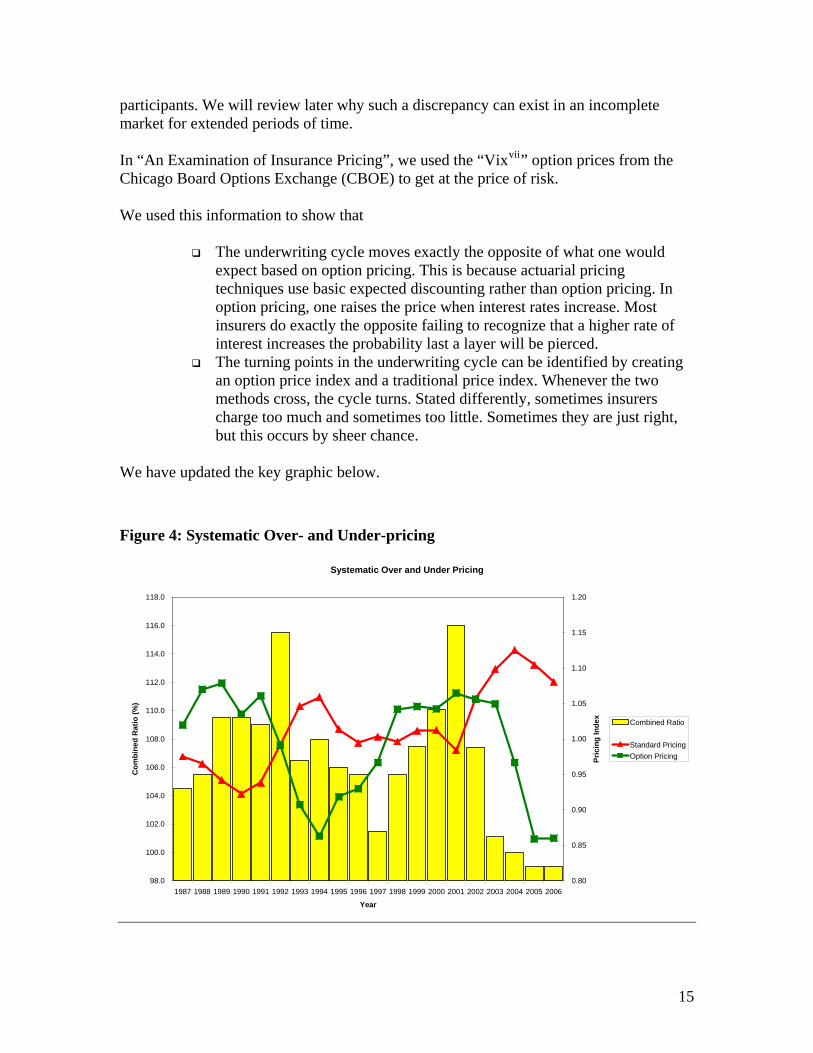
We have updated the key graphic below.
Figure 4: Systematic Over- and Under-pricing
Systematic Over and Under Pricing
98.0
100.0
102.0
104.0
106.0
108.0
110.0
112.0
114.0
116.0
118.0
1987 1988 1989 1990 1991 1992 1993 1994 1995 1996 1997 1998 1999 2000 2001 2002 2003 2004 2005 2006
Year
Com
bine
d R
atio
(%)
0.80
0.85
0.90
0.95
1.00
1.05
1.10
1.15
1.20Pr
icin
g In
dex
Combined Ratio
Standard PricingOption Pricing
15
As can be seen, the graphic looks one year ahead and suggests that the property and casualty insurance industry will have at least one more “good” year in terms of financial performance. This is because traditional pricing (red triangles) suggests a higher price than the option price (green squares) thus improving financial results. This graphic is interesting and thought-provoking, but the generality of it makes it difficult to demonstrate the value of our proposition without a doubt:
It is based on insurer’s reported results with the inherent lag in reporting and possible reserving bias.
The indexes do not propose a correct price per se. Rather they are based on a general model of the industry.
To address these and other questions, we reviewed actual data to develop a specific example of how an insurer would use this in practice.
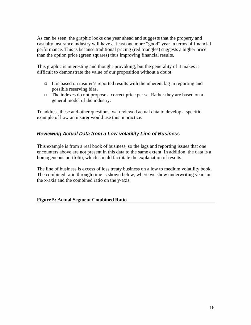
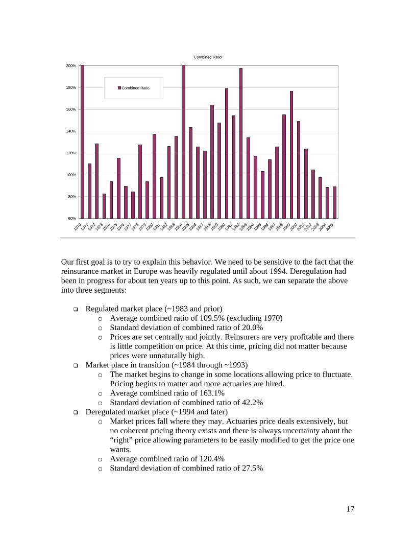
Reviewing Actual Data from a Low-volatility Line of Business This example is from a real book of business, so the lags and reporting issues that one encounters above are not present in this data to the same extent. In addition, the data is a homogeneous portfolio, which should facilitate the explanation of results. The line of business is excess of loss treaty business on a low to medium volatility book. The combined ratio through time is shown below, where we show underwriting years on the x-axis and the combined ratio on the y-axis.
Figure 5: Actual Segment Combined Ratio
16
Combined Ratio
60%
80%
100%
120%
140%
160%
180%
200%
1970
1971
1972
1973
1974
1975
1976
1977
1978
1979
1980
1981
1982
1983
1984
1985
1986
1987
1988
1989
1990
1991
1992
1993
1994
1995
1996
1997
1998
1999
2000
2001
2002
2003
2004
2005
Combined Ratio
Our first goal is to try to explain this behavior. We need to be sensitive to the fact that the reinsurance market in Europe was heavily regulated until about 1994. Deregulation had been in progress for about ten years up to this point. As such, we can separate the above into three segments:
Regulated market place (~1983 and prior) o Average combined ratio of 109.5% (excluding 1970) o Standard deviation of combined ratio of 20.0% o Prices are set centrally and jointly. Reinsurers are very profitable and there
is little competition on price. At this time, pricing did not matter because prices were unnaturally high.
Market place in transition (~1984 through ~1993) o The market begins to change in some locations allowing price to fluctuate.
Pricing begins to matter and more actuaries are hired. o Average combined ratio of 163.1% o Standard deviation of combined ratio of 42.2%
Deregulated market place (~1994 and later) o Market prices fall where they may. Actuaries price deals extensively, but
no coherent pricing theory exists and there is always uncertainty about the “right” price allowing parameters to be easily modified to get the price one wants.
o Average combined ratio of 120.4% o Standard deviation of combined ratio of 27.5%
17
Our focus will be on the latter two periods, as they are more indicative of the future. To set an option price structure for this segment, we need to estimate ground-up losses. Ideally, the ground-up distribution would be readily available, but in most cases, the current environment does not offer one. To develop a ground-up loss distribution, we define a few parameters that relate the ground-up loss distribution to the reinsurance distribution (which is readily available). Based on these parameters, the ground-up distribution will be entirely described.
( )( )RLGLa
ΕΕ
=1
( )GLAPa
Ε=2
)()(
)()(
RLRLStDev
GLGLStdev
fGroundUp
Ε
Ε=
Here, GL is the ground-up loss, RL is the reinsurance loss, and AP is the attachment point. In addition, we set
( )%900
0, =Ε
=i
ii RP
RLCR , where CR is the combined ratio, RL the reinsurance loss and RP
the reinsurance premium. The subscript i denotes the underwriting year.
yearst 4.4=Δ , which is the duration of the payout pattern. Note, that for simplicity we have included expenses in our ultimate loss estimate. This simplifies notation and has no further implications. The last two assumptions can be reviewed directly from the data. The first is the initial combined ratio estimate. In other words, how was the business viewed at the time it was underwritten? This may be directly available if the reinsurance data is complete from the date of inception. In our case, we have set it to 90% for all underwriting years consistent with the initial indications, though they will vary from underwriting year to underwriting
18
year. If the data is readily available by underwriting year, one can simply use it to get a more accurate result. The second is the duration of the business based on the claims payment pattern. This can be estimated directly from the payout pattern. This gives us an indication of how long it will take to pay out this business on average. We expect to make adjustments to our ultimate loss estimate for the same period of time on average. Given the mean and standard deviation of the ground-up log-normal distribution as well as the layer that is reinsured, one can determine the reinsurance expected loss and standard deviation (see Appendix). We can reverse this, so we find the ground-up mean and standard deviation given the reinsurance information. For any underwriting year, i, we have ( ) ii RPCRRL ⋅=Ε 0 ( ) ( ii RLaGL Ε⋅=Ε 1 )
)
( ) ( iii RLaaGLaAP Ε⋅⋅=Ε⋅= 122 ( )
( )( )
( )RLRLStDevf
GLGLStDev
GroundUp Ε⋅=
Ε
Thus, we now have to estimate 3 parameters to fully describe the value of the option: ,
, and . These can be estimated in a variety of ways. 1a
2a GroundUpf Any distributional assumption can be made at this point (unless the three parameters are directly available from existing data in which case one can avoid the restrictions of distributional assumptions), and the parameters found either through algebraic manipulation or through simulation. For our purposes, in order to estimate the parameters, we assume the ground-up loss is log-normal. This is consistent with the binomial lattice framework and the log-normal is commonly used in the insurance industry as an estimate of aggregate losses. Once the three parameters are given in addition to the reinsurance data, our ground-up distribution is entirely described. Once the parameters, and through them the ground-up distribution, have been found, pricing the option is a straight-forward exercise as laid out in our previous examples. But, it is important to recognize our previous work: The price of risk differs over time. As such, for pricing purposes, there is not a constant volatility. It fluctuates and we can use our price of risk concept to recognize this. In our original paper, we defined a price of risk as volatility relative to return. The required us to estimate a coefficient of variation for insurance, which includes the
19
estimation of a return (e.g. “drift” in reserve estimates) in insurance. There are two pro m
The results are very sensitive to the mean return
uce our new price of risk as a “Price of Risk Factor” or is simply a scaling factor of volatility measured by the current value of vix relative to
its trailing historical average.
ble s with this:
We know from options theory that the return does not matter Accordingly, we will now modify our concept of the price of risk. It is important to note,that is leaves our original work intact albeit with different parameters. In other words, the graph in the previous section (Figure 4) can be reproduced in the following framework. To avoid confusion, we introd *λ . It
vixvixt
t =*λ ,
where N
vixN
tt∑
=1
hatever volatility we get for the ground-up loss, we will rescale it based on our “Price of Risk Factor”.
, where
vix =
W
*
, tGroundUptGroundUp λσσ ⋅= GroundUpσ is the actuarial estimate of volatility of the
to s
es sense since this is a irly homogeneous portfolio. Given complete data and an individual treaty, the
ould be explicit by treaty by underwriting year.
ground-up loss. To test our theory further, we find the parameters 1a , 2a , and GroundUpf through a minimum sum of squared errors approach. Stated differently, since we are trying understand the underwriting cycle, we simply let our history of combined ratios tell uwhat reasonable assumptions for our three parameters would be. We assume the parameters are the same for each underwriting year. This makfaparameters w Hypothesis Traditional insurance pricing does not properly account for the optionality inherent in insurance contracts. As such, insurance contracts can be arbitraged thus extending losses when prices are low relative to the arbitrage-free price. Thus, we should be able to
ow that the combined ratio tends to be extended when the arbitrage-free price is high ve to the traditional (actual) price.
shrelati
Test
Minimize ∑ ⎟⎟=
⎞⎜⎛
−I
i
iCCR
2
, where
⎠
⎜⎝ i
i P1
20
We allow losses to be rescaled to get the best fit possible The adj usted option price is the option price incorporating our Price of Risk Factor
Here,
m o ing the ground-up log-normal distribution as described by parameters , and
P is the actual reinsurance premium for underwriting year i.
our case, we get the following results:
r values that best describe the available data. As such, they o not have to be observable.
he graph below summarizes the results.
igure 6: Combined Ratio versus Pricing Methods
CRi is the reinsurance combined ratio for underwriting year i, Ci is the call option (reinsurance) price as laid out in our pricing fra ew rk (us
1a , 2a
GroundUpf ), and i
In
%6.9%5.90
%5.9
2
1
===
GroundUpfaa
Reviewing these for reasonability, they do not seem unreasonable. One could argue thatthey do not even have to be reasonable per se, as they are akin to state variable pricing factors or simply the parameted T
F
21
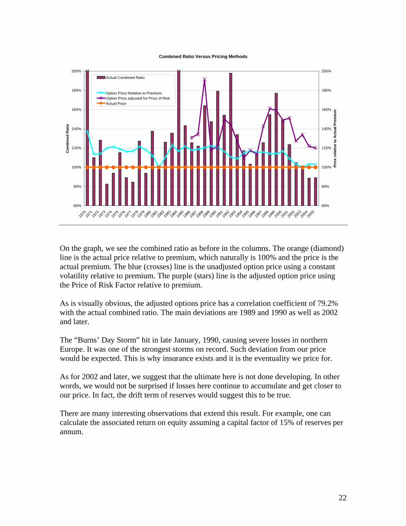
Combined Ratio Versus Pricing Methods
160%
180%
200%
180%
200%
120%
140%
Com
bine
d R
atio
140%
ve to
Act
ual P
r
80%
100%
80%
100%
60%
1970
1971
1972
1973
1974
1975
1976
1977
1978
1979
1980
1981
1982
1983
1984
1985
1986
1987
1988
1989
1990
1991
1992
1993
1994
1995
1996
1997
1998
1999
2000
2001
2002
2003 00
4 05
60%
2 20
120%
160%
Pric
e re
lati
emiu
m
Actual Combined Ratio
Option Price Relative to PremiumOption Price adjusted for Price of RiskActual Price
On the graph, we see the combined ratio as before in the columns. The orange (diamond) line is the actual price relative to premium, which naturally is 100% and the price is the ctual premium. The blue (crosses) line is the unadjusted option price using a constant
volatility relative to premium. The purple (stars) line is the adjusted option price using the Price of Risk Facto tive to premium. As is visually obvious, the adjusted options price has a correlation coefficient of 79.2%
ith the actual combined ratio. The main deviations are 1989 and 1990 as well as 2002
ould be expected. This is why insurance exists and it is the eventuality we price for.
s for 2002 and later, we suggest that the ultimate here is not done developing. In other ords, we would not be surprised if losses here continue to accumulate and get closer to
our price. In fact, the drift term of reserves would suggest this to be true. There are many interesting observations that extend this result. For example, one can calculate the associated return on equity assuming a capital factor of 15% of reserves per annum.
a
r rela
wand later. The “Burns’ Day Storm” hit in late January, 1990, causing severe losses in northern
urope. It was one of the strongest storms on record. Such deviation from our price Ew Aw
22
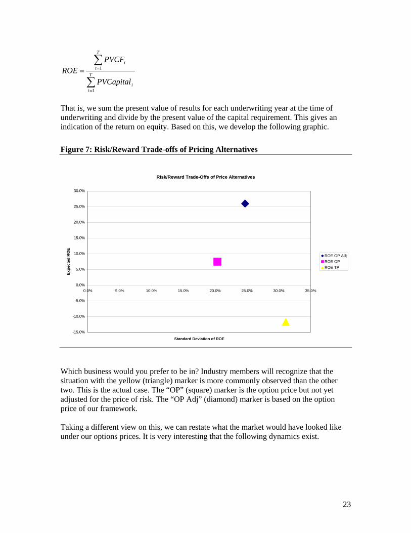
∑
∑
=
== T
ti
T
tt
PVCapital
PVCFROE
1
1
That is, we sum the present value of results for each underwriting year at the time of underwriting and divide by the present value of the capital requirement. This gives an indication of the return on equity. Based on this, we develop the following graphic.
Figure 7: Risk/Reward Trade-offs of Pricing Alternatives
Risk/Reward Trade-Offs of Price Alternatives
-15.0%
0.0%
5.0%
10.0%
0.0% 5.0%
Expe
cted
RO
E
15.0%
20.0%
25.0%
30.0%
10.0% 15.0% 20.0% 25.0% 30.0% 35.0%
ROE OP AdjROE OPROE TP
-10.0%
-5.0%
Standard Deviation of ROE
Which business would you prefer to be in? Industry members will recognize that the
is more commonly observed than the other o. This is the actual case. The “OP” (square) marker is the option price but not yet
djusted for the price of risk. The “OP Adj” (diamond) marker is based on the option
aking a different view on this, we can restate what the market would have looked like
situation with the yellow (triangle) markertwaprice of our framework. Tunder our options prices. It is very interesting that the following dynamics exist.
23
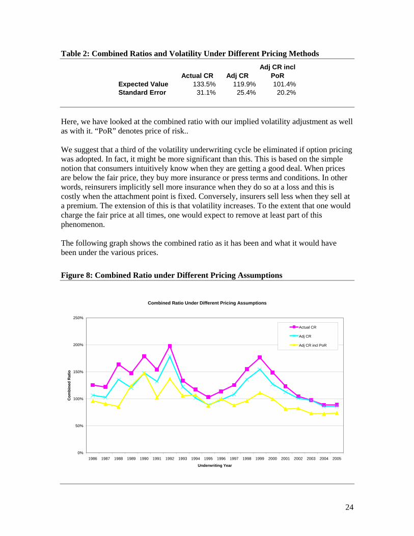
Table 2: Combined Ratios and Volatility Under Different Pricing Methods
Actual CR Adj CRAdj CR incl
PoRExpected Value 133.5% 119.9% 101.4%Standard Error 31.1% 25.4% 20.2%
Here, we have looked at the combined ratio with our implied volatility adjustment as well
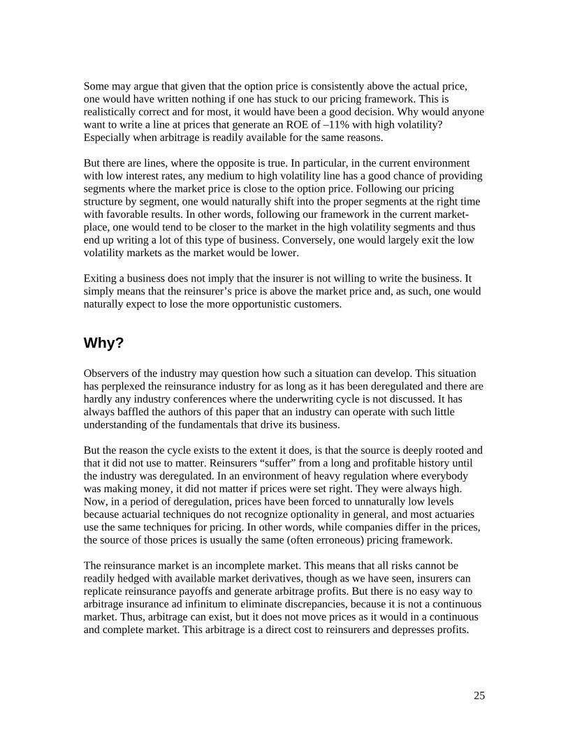
e suggest that a third of the volatility underwriting cycle be eliminated if option pricing was adopted. In fact, it might be more significant than this. This is based on the simple notion that consumers intuitively know when they are getting a good deal. When prices are below the fair price, they buy more insurance or press terms and conditions. In other words, reinsurers implicitly sell more insurance when they do so at a loss and this is costly when the attachment point is fixed. Conversely, insurers sell less when they sell at a premium. The extension of this is that volatility increases. To the extent that one would charge the fair price at all times, one would expect to remove at least part of this phenomenon. The following graph shows the combined ratio as it has been and what it would have been under the various prices.
Figure 8: Combined Ratio under Different Pricing Assumptions
as with it. “PoR” denotes price of risk.. W
Combined Ratio Under Different Pricing Assumptions
200%
250%
Actual CR
Adj CR
0%
50%
1986 1987 1988 1989 1990 1991 1992 1993 1994 1995 1996 1997 1998 1999 2000 2001 2002 2003 2004 2005
Underwriting Year
Adj CR incl PoR
100%
150%
Com
bine
d R
atio
24
Some may argue that given that the option price is consistently above the actual price, one would have written nothing if one has stuck to our pricing framework. This is realistically correct and for most, it would have been a good decision. Why would anyone
ant to write a line at prices that generate an ROE of –11% with high volatility? Especially when arbitrage is readily available for the same reasons.
re lines, where the opposite is true. In particular, in the current environment
hus e would largely exit the low
ld
on e
ut the reason the cycle exists to the extent it does, is that the source is deeply rooted and until
ces have been forced to unnaturally low levels ecause actuarial techniques do not recognize optionality in general, and most actuaries
es,
n its. But there is no easy way to
rbitrage insurance ad infinitum to eliminate discrepancies, because it is not a continuous
its.
w
ut there aB
with low interest rates, any medium to high volatility line has a good chance of providingsegments where the market price is close to the option price. Following our pricing structure by segment, one would naturally shift into the proper segments at the right time with favorable results. In other words, following our framework in the current market-place, one would tend to be closer to the market in the high volatility segments and tnd up writing a lot of this type of business. Conversely, one
volatility markets as the market would be lower. Exiting a business does not imply that the insurer is not willing to write the business. It simply means that the reinsurer’s price is above the market price and, as such, one wounaturally expect to lose the more opportunistic customers.
Why? Observers of the industry may question how such a situation can develop. This situatihas perplexed the reinsurance industry for as long as it has been deregulated and there arhardly any industry conferences where the underwriting cycle is not discussed. It has always baffled the authors of this paper that an industry can operate with such little understanding of the fundamentals that drive its business. Bthat it did not use to matter. Reinsurers “suffer” from a long and profitable historythe industry was deregulated. In an environment of heavy regulation where everybodywas making money, it did not matter if prices were set right. They were always high. Now, in a period of deregulation, pribuse the same techniques for pricing. In other words, while companies differ in the pricthe source of those prices is usually the same (often erroneous) pricing framework. The reinsurance market is an incomplete market. This means that all risks cannot be readily hedged with available market derivatives, though as we have seen, insurers careplicate reinsurance payoffs and generate arbitrage profamarket. Thus, arbitrage can exist, but it does not move prices as it would in a continuous and complete market. This arbitrage is a direct cost to reinsurers and depresses prof
25
How can this exist? In an incomplete market, participants are cursed (or blessed p e to
oneself. This is not a new concept.
ants
y have nothing to base it on.
ound that incomplete markets stay incomplete while omplete markets quickly converge to efficiency (even with few participants). It is
hat really was interesting to Prof. Smith was the fact that given the choice, incomplete
f
o, there is a human comfort in being able to make up the truth such that it suits oneself. But, it is not very profitable.
but given that we are in an incomplete
depending on your perspective) by not knowing the truth. As such, they can make utheir own truth and our survival instinct usually makes such truth one that is favorabl
In an inefficient and incomplete market, participants can delude themselves. A recent study by McKinsey & Co. found that 80% of insurance CEOs believed that they would do the right thing in the next down market. But only 20% believed that other participwould… This is reminiscent of the classic introductory psychology course scenario where 80% of a given pool of participants think they are above average, though – or rather because - the Similarly, a behavorial study by Professor Vernon Smith compared aspects of complete and incomplete markets and fcimportant to note his definitions of a complete and incomplete market: Complete: Continuous two-sided bid-ask system such as electronic exchanges. Incomplete: Bilateral markets, where buyers and sellers find each other and make
direct contact. Wmarket participants chose to stay with the incomplete market. Not knowing any better, they simply had “lots of confidence to just go it alone. We have a long way to go to understand this choice.” He calls this “survival economics” rather than “maximization oprofits”. Though he never specifically mentions the reinsurance market, the authors find the parallels eerie. S
hange will necessarily come at some point,C
market and that this scenario is itself fairly stable, we need a pivotal event. A pricing theory and framework such as what we are proposing here could go a long way. Also, change of the market structure could facilitate. As more existing (run-off) insurance losses are traded, it is plausible that a bid-ask exchange could be developed that would pill over to the current market place. s
The parallels here between the insurance market of today and the options market of 30 years ago are interesting. Prior to the emergence of the Chicago Board Options Exchange (CBOE) and the Black-Scholes option theory, options pricing was hardly as organized and straight-forward as it is today. A similar exchange for insurance risk combined with a coherent theory of pricing could do wonders to the viability of the industry in the long-erm. t
26
Summary and Conclusion
e have described in deW tail the underwriting cycle of the industry in general as well as a
o
g loss estimates will develop like a lattice with factor u and d=1/u. This ould force a price rigor and structure that would at the same time make arbitrage against e insurer more difficult. The main parameter to estimate is the volatility and the result is
ot as sensitive to changes in this parameter as traditional pricing is to changes in other istributional parameters.
e have also shown that reinsurance can be replicated with direct insurance, and that this eans that insurance can actually be arbitraged. But the market remains incomplete and e have explained this.
he reinsurance market needs to be more complete. Further product development is needed for this to develop, but a coherent pricing theory is missing to set the structure around the pricing of the financial products. We have shown that option theory can be applied successfully to accomplish this and hope to see more products introduced with this in mind.
specific segment. We have shown that our hypothesis explains more than 60% of thevariation in the underwriting cycle and that the industry would generate returns closer twhat one would expect given the level of risk, if it were to follow our framework. We have showed that any reinsurer or insurer would be well served to price assuming hat underlyint
wthnd Wmw T
27
Appendix
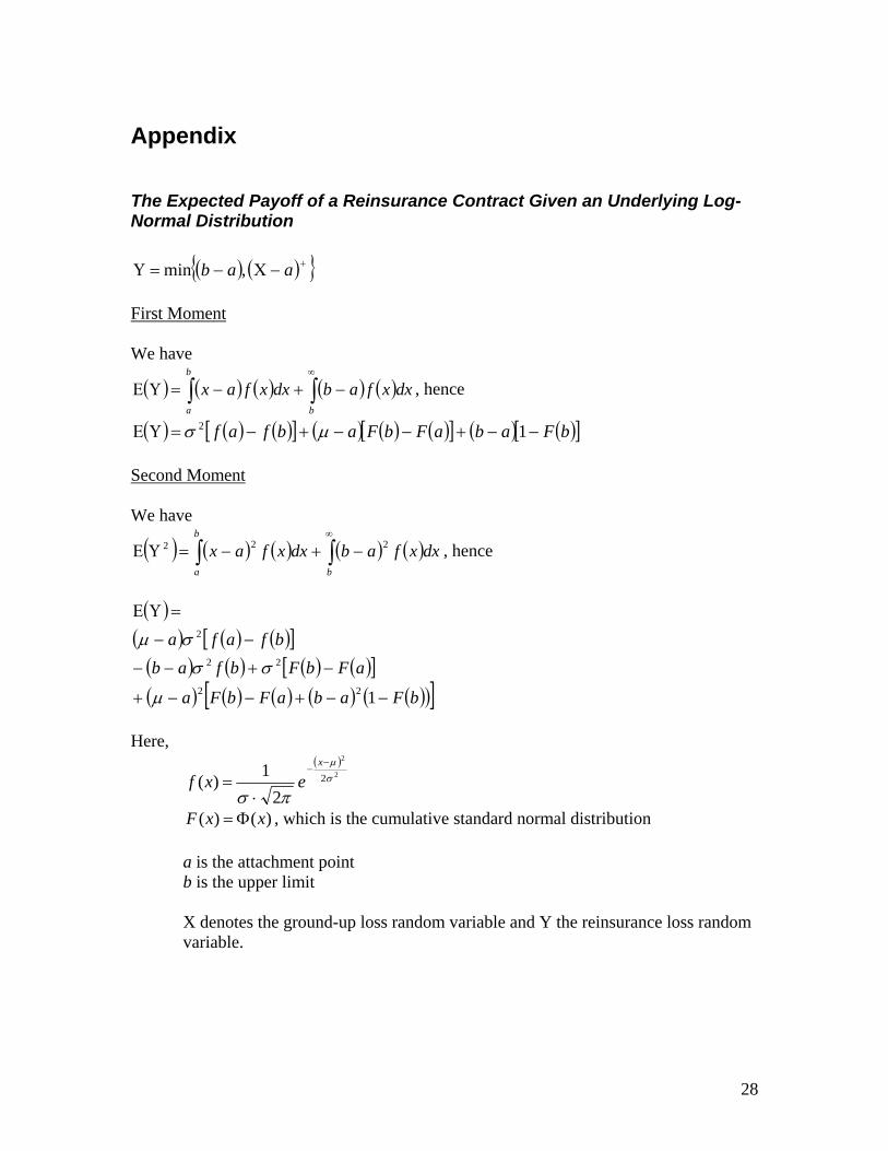
The Expected Payoff of a Reinsurance Contract Given an Underlying Log-Normal Distribution
( ) ( ){ }+−Χ−=Υ aab ,min First Moment We have
( ) ( ) ( ) ( ) ( )∫∫∞
−+−=ΥΕb
b
a
dxxfabdxxfax , hence
( ) ( ) ( )[ ] ( ) ( ) ( )[ ] ( ) ( )[ ]bFabaFbFabfaf −−+−−+−=ΥΕ 12 μσ Second Moment We have
( ) ( ) ( ) ( ) ( )∫∫∞
−+−=ΥΕb
b
a
dxxfabdxxfax 222 , hence
( )
( ) ( ) ( )[ ]( ) ( ) ( ) ( )[ ]( ) ( ) ( ) ( ) (( )[ ]bFabaFbFa
aFbFbfabbfafa
−−+−−+
−+−−
−−
=ΥΕ
122
22
2
μ
σσ
σμ
)
Here,
( )2
2
2
21)( σ
μ
πσ
−−
⋅=
x
exf
)()( xxF Φ= , which is the cumulative standard normal distribution a is the attachment point b is the upper limit X denotes the ground-up loss random variable and Y the reinsurance loss random variable.
28
References A.M. Best Company, “Discipline and Specialized Distribution Are Keys to Program Underwriters' Success”, February 1, 1999 Special Report Arnold, Tom and Crack, Timothy: “Using the WACC to Value Real Options”, Financial Analysts Journal, Vol. 60, No. 6, November/December 2004 Black, Fischer and Scholes, “The Pricing of Options and Corporate Liabilities”, Journal of Political Economy, 81:3, 1973, pp. 637-654 Ciezadlo, Greg, “Market Cycle Update, Personal Lines”, CAS Spring Meeting, 2002 Commerce Department's National Institute of Standards (NIST) and International Sematech (IST), “E-Handbook of Statistical Methods” Embrechts, Paul: “Actuarial versus financial pricing of insurance”, Swiss Institute of Technology, Switzerland Fenn, Paul: “Round and Round – some of the theoretical explanations of the underwriting cycle”, www.globalreinsurance.com Gerber and Pafumi: “Utility Functions: From Risk Theory to Finance”, North American Actuarial Journal, 1998, Volume 2, Number 3. Harrington, Cynthia, “Beyond Belief – Pioneering Insights Into Behavioral Finance”, CFA Magazine, September/October 2003 Hull, John C., “Options, Futures, and Other Derivatives”, Prentice Hall, 1997 Insurance Information Institute Insurance Journal, "”Combined Ratio for 2001 on Track to Hit Record High, ISO President Says”, Property and Casualty Magazine, April 2001 James, Julian, “The challenge for change”, Speech at ILICA conference, 29 September 2004 James, Kaye D. and Oakley, David, “Underwriting Cycles by Kaye D. James - Discussion by David J. Oakley” Luenberger, David, “Investment Science”, Oxford University Press, 1998 Mack, Thomas, “Distribution-free calculation of the standard error of chain-ladder
29
reserve estimates”, ASTIN Bulletin, 23, 1993, pg. 213-225 Madsen, Chris and Pedersen, Hal: “An Examination of Insurance Pricing and Underwriting Cycles”, AFIR Colloquium, September, 2003, pg 769-794 Mitchell, Roger, “A Model Mind – Robert C. Merton on Putting Theory into Practice”, CFA Magazine, July-August, 2004 Moore, James, “Hard Markets”, RiskIndustry.com, August 25, 2001 Sepp, Thomas and Bate, Oliver, “The Underwriting Cycle – a phenomenon to be controlled, not endured”, McKinsey & Company, November 27, 2003 Sherris, Michael: “Solvency, Capital Allocation and Fair Rate of Return in Insurance”, UNSW, Sydney, Australia, January, 2004 Skurnick, David, “The Underwriting Cycle”, CAS Underwriting Cycle Seminar, April, 1993 Swiss Re, “Deregulation and liberalisation of market access: the European insurance industry on the threshold of a new era in competition”, sigma No. 7/1996 Swiss Re, “Profitability of the non-life insurance industry: it's back-to-basics time”, Sigma, No. 5/2001 Swiss Re, “Reinsurance – a systematic risk?”, Sigma, No. 5/2003 Tarashev, Nikola et al: “Investors’ attitude towards risk: what can we learn from options?”, BIS Quarterly Review, June 2003 Verall, R.J.: “Obtaining Predictive Distributions for Reserves which Incorporate Expert Opinion”, CAS Forum, 2004 Wang, Shaun: “A Universal Framework for Pricing Financial and Insurance Risks” i To see this, graph the payoff function of an excess of loss contract. It is exactly the payoff of a call option. ii In continuous time, this becomes Brownian motion, which can be described as
dzdtL
dL⋅+⋅= σμ .
30
iii Note, that many distributions can be explained by changing u’s and d’s in the binomial lattice. iv Volatility of ultimate reserves will generally range from 0% to 60+% depending on line of business. v If p=50% and ⎟
⎠
⎞⎜⎝
⎛Ε=RL
L P 10 , then d=2R-u.
vi For more detail on this, please see Madsen and Pedersen 2003. vii The CBOE Volatility Index - more commonly referred to as "VIX" - is an up-to-the-minute market estimate of expected volatility that is calculated by using real-time S&P 500 (SPX) index option bid/ask quotes. VIX uses nearby and second nearby options with at least 8 days left to expiration and then weights them to yield a constant, 30-day measure of the expected volatility of the S&P 500 Index. The underlying for options is an "Increased-Value" Volatility Index (VXB), which is calculated at 10 times the value of VIX. For example, when the level of VIX is 12.81, VXB would be 128.10.
31