« A Fresh Scrutiny on Openness and

Per Capita Income Spillovers in Chinese

Cities: A Spatial Econometric Perspective »

Selin OZYURT

DR n°2008-17

1

A Fresh Scrutiny on Openness and Per Capita Income Spillovers in

Chinese Cities: A Spatial Econometric Perspective

Selin Ozyurt

November 2008

Abstract

This paper investigates openness and per capita income spillovers over 367 Chinese cities in the year 2004. Per capita income is modelled as dependent on investment, physical and social infrastructure, human capital, governmental policies and openness to the world. Our empirical analysis improves substantially the previous research in several respects: Firstly, by extending the data set to prefecture-level, it tackles the aggregation bias. Secondly, the introduction of recently developed explanatory spatial data analysis (ESDA) and spatial regression techniques allows to address misspecification issues due to spatial dependence. Thirdly, the endogeneity problem in the regression is taken into consideration through the use of generalised method of moments (GMM) estimator. Our major findings are in Chinese cities, physical and social infrastructure development, human capital and investment could be recognised as major driving sources of per capita income (i), whereas, the government expenditure ratio exerts a negative impact on per capita GDP level (ii). Our empirical findings also yield evidence on the existence of FDI and foreign trade spillovers in China (iii). These findings are robust to a number of alternative spatial weighting matrix specifications. Keywords: China, openness, spatial regression, spillovers, transition economies.

JEL Classification: O11, O18, P24, R10.

2

1. INTRODUCTION

Since the introduction of the economic reform policy in the early 1980’s, China has been

experiencing a continuous rapid economic growth. Alongside the implementation of market

oriented policies, China has progressively emerged in the world economy as a major global

economic partner. In 2002, China overtook the United States and became the largest recipient

of foreign direct investment (FDI) in the world. Moreover, in 2006, it outpaced major trading

countries and turned to be the world’s 3rd largest trading partner.

In China, the transition from an autarchic to a market economy has been a gradual and

spatially uneven process. Differences in regional resource endowments as well as opening up

policies which favoured coastal regions lead to dramatic disparities in regional development

paths.

The purpose of this study is to bring new insight to our understanding of China’s recent

economic performances. Based on a comprehensive data set, this study yields fresh empirical

evidence to a number of questions: What are the driving forces behind China’s recent

economic development? What is the spatial pattern of China’s per capita income distribution?

To what extent the opening-up policies contribute to regional economic development of

China? Are there any spillovers resulting from FDI and international trade?

This study improves substantially previous literature in several respects: First, in order to

address any aggregation biases, it extends the cross-sectional basis to prefecture-level data.

Due to data limitations, the existing literature on China’s regional development is confined to

province-level data. However, given the massive size of China, one can expect that using

smaller scale spatial units would provide a better understanding of regional development

patterns (Yu and Wei, 2008).

Second, the paper addresses spatial effects in the regression analysis by the explicit

incorporation of spatial information in the modeling scheme. We consider that for a better

understanding of regional development, the focus should be put on spatial patterns and

interactions among geographical units. Moreover, ignoring spatial autocorrelation might lead

3

to serious misspecification issues, inconsistent parameter estimates and statistical inferences

(Anselin, 1988).

Third, previous studies generally overlook the endogeneity issue. However while

investigating the contribution of openness to economic development, a potential inverse

causality should also be taken into consideration. In this study, we tackle the endogeneity

issue through the use of the GMM estimator.

The remainder of the paper proceeds as follows. The second section presents the underlying

data set and methodology. Spatial effects are outlined and discussed in section 3. Section 4

presents the empirical outcomes. The last section concludes the paper.

2. METHODOLOGY

Our investigation of China’s economic development is mainly inspired from the endogenous

growth framework (Lucas, Romer). Following the empirical literature (Wei 2000; Yu and

Wei 2008), we chose per capita GDP as an indicator of regional development. It can be

clearly observed from Figure 1 that per capita income exhibits striking disparities among

sample cities.

Figure 1: Distribution of GDP per capita in sample cities (2004).

2.1. Data

The underlying data is collected from China Provincial Statistical Yearbook (2005) from 31

provinces. The data set covers 364 county and prefecture-level cities and 3 super cities

4

(Beijing, Tianjin, Shanghai) spread over the entire Chinese territory. After excluding

observations with missing values our final sample includes 367 cities for the year 2004 (see

Appendix Table A1).

2.2. Model

The dependent we use, is the ratio of GDP to population at the year-end. The set of control

variables is specified as follows: Physical capital accumulation is proxied by the ratio of

completed investment in capital construction to population (INV). The ratio of number of

beds in hospitals and sanitation agencies to population (Bed) proxies for social infrastructure.

Physical infrastructure is quantified through the ratio of local telephone subscribers to

population (Phone). The human capital variable is the ratio of student enrollment in regular

secondary schools to population (HK). Openness is measured by the ratios of exports value to

GDP (EXP) and foreign capital actually used to GDP (FDI). Political determinants are

controlled by local government expenditure to GDP ratio (GVT). Table A2 summarizes a

basic description of model series. After the log linear transformation, the model could be

expressed as follows:

iii

iiiiiii

EXPPhoneFDIGVTHKBedInvGDP

εαααααααα

++++++++=

76

543210

lnlnlnlnlnlnln

(1)

3. SPATIAL EFFECTS

Spatial econometrics takes its origins from Tobler’s first law of geography (1970):

« Everything is related to everything else, but near things are more related than distant things

». Spatial econometrics is dedicated to the study of spatial structure and spatial interactions

between observation units. It is mainly inspired from the research issues of new economic

geography and regional science (Anselin, 2001). The main distinguishing characteristic of

spatial data analysis is taking into account the spatial arrangement of observations. That is to

say, regions are not treated as isolated economies; the interactions between them are

explicitly incorporated into the modelling scheme. Since the last decade, the increasing

availability of geo-referenced socio-economic data sets made possible the extension of

applied spatial econometrics studies to more traditional fields of economics (e.g. international

economics, labour economics, public economics, agricultural and environmental economics).

In addition, since few years, the time dimension has also started to be included in spatial

modelling (see Ehorst 2001, Anselin and Le Gallo, 2008)

5

3.1. Spatial Dependence

Spatial dependence (or spatial autocorrelation) is one of the main issues introduced by the use

of geographic data. It refers to absence of independence between geographic observations. In

other words, spatial autocorrelation corresponds to the coincidence of value similarity and

location similarity (Anselin, 2001).

Spatial dependence could arise from either theoretical or statistical issues. On one hand, it

could be the outcome of the integration of geographical units due to labour migration, capital

mobility, transfer payments and inter-regional trade. It can also arise from some institutional

and political factors and externalities such as technology diffusion and knowledge spillovers

(Buettner, 1999; Ying, 2003). On the other hand, spatial dependence could be related to some

statistical issues such as measurement errors, varying aggregation rules, different sample

designs and omission of some variables with spatial dimension (e.g. climate, topology and

latitude) (Anselin and Florax, 1995).

3.2. Spatial weighting matrix The spatial weighting matrix provides the structure of assumed spatial relationships and

captures the strength of potential spatial interactions between observation units. Thereby, in

spatial analysis, constructing appropriate spatial weighting matrices is of particular

importance. The choice of the spatial matrix could affect both the performance of spatial

diagnostic tests and estimated parameters. Given that the elements of the spatial weights

matrix are expected to be exogenous to the model (otherwise the model would be highly non

linear), in the literature, the weighting matrix is generally based on geographic contiguity

based on border sharing or distance.

• Simple contiguity:

The binary contiguity matrix is widely used in the literature due to its simplicity of

construction. It is based on the adjacency of locations of observations. Put wij to express the

magnitude of the interaction between provinces i and j. Then, if two provinces share a

common boundary wij=1 and wij=0 otherwise.

• Distance based contiguity:

In distance based contiguity matrices, spatial weights attributed to observations depend on

geographic distance dij between locations i an j. Distance matrices differ in functional form

6

used, distance function [wij=dij], inverse function of distance [wij =1/dij ], inverse distance

raised to some power [wij =1/dijN] and negative exponential function [wij =exp(-θdij)] are

mostly used in the literature. In distance decay functions, the strength of spatial interactions

decline with geographic distance. dij corresponds to the cut-off point which maximizes the

spatial association and beyond which spatial interactions between units are assumed to be non

existent. In the literature, cut-off points are generally set up following some statistical or

arbitrary criterions such as minimum or median distance between regions, the significance of

spatial diagnostic statistics, and goodness of fit of the regression.

The weighting matrix is generally row standardised by dividing each weight of an

observation by the corresponding row sum wij / Σ j wij. Thereby, the elements of each row sum

to unity1 and each weight wij could be interpreted as the province’s share in the weighted

average of neighbouring observations. wij=0 indicates lack of spatial interactions between

observations. By convention, distance matrix has zeros on the main diagonal, thus no

observation predicts itself.

Given the complexity of interactions among geographic units, in this study, we explore the

robustness of our results with respect to various specifications of distance weighting matrix.

On this purpose, six spatial weights matrices are constructed based on either border sharing or

distance based contiguity. The main characteristics of the Euclidian distance matrix for our

sample are summarised in Table A3. We set the minimum upper distance band to 10

kilometres regarding the minimum allowable distance cut-off point (9.33 kilometers).

In spatial econometrics explanatory spatial data analysis (ESDA) techniques are used for

univariate level analysis while, spatial regression techniques allow to explore spatial patterns

for multivariate level. Recent literature (Anselin, 2001) provides taxonomy of spatial

econometric models. In this study, our focus will be limited to two major spatial modeling

schemes, namely spatial lag and spatial error models.

3.3. Spatial Regressions

• Spatial Lag:

1 Whereas the original spatial weighting matrix is usually symmetric, the row-standardised one is not (Anselin and LeGallo, 2008). An asymmetric spatial weighting matrix implies that, region i could have a larger influence on the random variable of interest in region j and vice-versa.

7

The spatial lag model combines the standard regression model with a spatially lagged

dependent variable introduced as an explanatory variable. Spatial lag operators refer to a

weighting average of random variables in proximate regions. Spatial lag model could be

expressed as below:

εβρ ++= XWyy (2)

Using traditional notation, y is a (N x 1) vector of observations of dependent variable, X, a (N

x K) matrix of K exogenous variables, β, a (K x 1) vector of explanatory variable coefficients

and ε, a (N x 1) vector of stochastic disturbance terms. W corresponds to a (N x N) spatial

weighting matrix which identifies the geographic relationship among spatial units. ρ refers to

spatial autoregressive parameter that captures spatial interactions between observations. It

measures the impact of surrounding regions (positive or negative) on the dependent variable

in a reference region i. ρ is assumed to lie between -1 and 1. If ρ≠0, ignoring ρ have similar

consequences to omitting a significant independent variable in the regression model. That is

to say, the statistical inferences and estimated parameters would be questionable.

In spatial lag model, including a spatially lagged dependent variable in the right hand side

introduces a simultaneity problem. By construction, the lagged dependent variable is

correlated with the individual fixed effects in the error term. Consequently, the OLS estimator

becomes inconsistent and biased. In the literature the endogeneity problem is corrected via

instrumental variables, maximum likelihood (ML) estimator or generalised method of

moments (GMM) estimator (see Kelejian and Prucha, 1999).

• Spatial Error Model:

In spatial error model, spatial autoregressive process is confined to the error term. Spatial

error models can be represented in the following form:

εβ += Xy (3)

μελε += W then 1)( −−= WI λε (4)

Where ε, a (Nx1) element vector of error terms and λ the spatial autocorrelation coefficient

which is assumed to lie between -1 and 1. The parameter λ captures how a random shock in a

specific region is propagated to surrounding regions. By definition, the spatial lag term Wε is

clearly endogenous and correlated with the error term. Living out spatial correlation between

error terms has similar consequences to ignoring heteroscedasticity. That is to say, the OLS

8

estimator remains consistent but no longer efficient (it might lead to biased and inconsistent

statistical inferences).

3.4. The diagnostic of spatial dependence

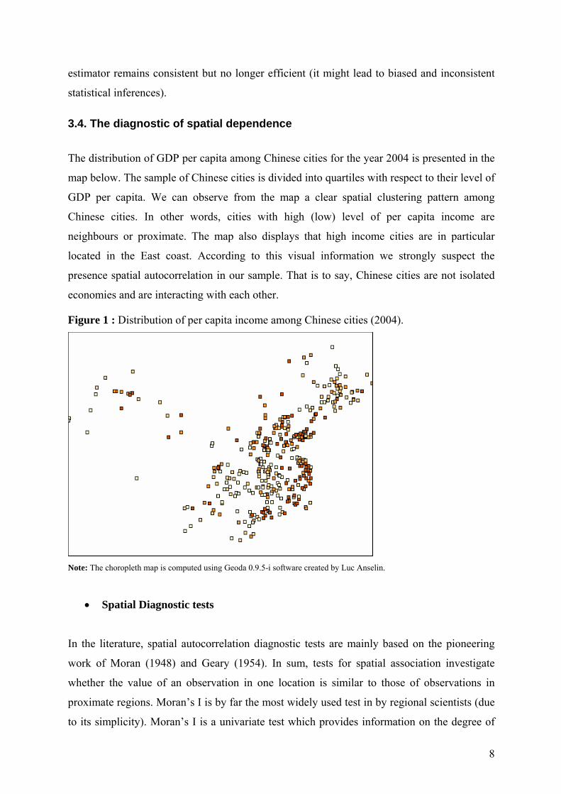
The distribution of GDP per capita among Chinese cities for the year 2004 is presented in the

map below. The sample of Chinese cities is divided into quartiles with respect to their level of

GDP per capita. We can observe from the map a clear spatial clustering pattern among

Chinese cities. In other words, cities with high (low) level of per capita income are

neighbours or proximate. The map also displays that high income cities are in particular

located in the East coast. According to this visual information we strongly suspect the

presence spatial autocorrelation in our sample. That is to say, Chinese cities are not isolated

economies and are interacting with each other.

Figure 1 : Distribution of per capita income among Chinese cities (2004).

Note: The choropleth map is computed using Geoda 0.9.5-i software created by Luc Anselin.

• Spatial Diagnostic tests

In the literature, spatial autocorrelation diagnostic tests are mainly based on the pioneering

work of Moran (1948) and Geary (1954). In sum, tests for spatial association investigate

whether the value of an observation in one location is similar to those of observations in

proximate regions. Moran’s I is by far the most widely used test in by regional scientists (due

to its simplicity). Moran’s I is a univariate test which provides information on the degree of

9

linear association between proximate observations. In general, spatial diagnostic tests are

conducted under the null hypothesis of lack of model misspesification due to spatial

dependency. The significance of the coefficient is based on z-values. Anselin (1995) has also

developed a local indicator of spatial correlation (LISA) which provides a spatial association

measure for a particular locality and identifies local clusters. Cliff and Ord (1981) adopted

Moran’s I test to regression residuals to detect spatial autocorrelation in multivariate level.

In order to detect a possible spatial dependence in the model, we perform Moran’s I test for

regression residuals. Table 1 reports the results of Moran’s I statistic and associated

probabilities with respect to six weighting matrices. Spatial diagnostic tests reveal a clear

positive spatial autocorrelation process. Consequently, we reject the null hypothesis that in

China economic development of cities is randomly distributed over space.

After identifying the presence of spatial dependence, we need to specify the adequate

underlying structure of spatial dependence. On this purpose, we perform LM test which

allows to distinguish between two alternative specifications of spatial models namely spatial

error and spatial lag. The choice of the most adequate model is operated by the joint use of

the LMERR and LMLAG statistics. According to the decision rule proposed by Anselin and

Florax (1995) the model with the highest value (or lowest probability) should be chosen. In

our case, according to the results of LM and robust LM tests presented in Table 1, spatial

effects in the form of spatially lagged dependent variable (the SAR model) seems to fit better

the underlying spatial structure.

Table 1: Diagnostic tests for spatial dependence

Binary D10 D25 D50

D75 D100Morans’s I 6.023

[0.000] 4.116

[0.000]4.618

[0.000]4.548

[0.000]4.586

[0.000] 6.070

[0.000]LMSAR 79.420

[0.000] 49.239[0.000]

49.263[0.000]

48.111[0.000]

48.768 [0.000]

82.579[0.000]

LMERR 32.536 [0.000]

14.978[0.000]

18.730[0.000]

18.054[0.000]

18.328 [0.000]

32.514[0.000]

LMSAR Robust

6.972 [0.008]

9.543[0.002]

9.139[0.002]

8.894[0.002]

7.837 [0.005]

8.808[0.002]

LMERR Robust

5.760 [0.016]

0.317[0.573]

0.882[0.347]

0.815[0.366]

1.114 [0.291]

3.766[0.052]

Notes: Figures in brackets are probabilities. All spatial weights matrices are row-standardized: Binary is the first order contiguity; D10 refers to distance-based contiguity for a distance band of 0-10 km and so on. The tests are performed by using MATLAB program spatial econometrics toolbox of Lesage (www.spatial-econometrics.com).

10

4. Results In this section, we augment Equation 1 by introducing a spatial lag component WlnGDPi.

Accordingly, we consider that due to spatial interactions and clustering phenomenon, per

capita income in a given city could be affected by per capita income in neighbour or

proximate cities. The spatial model we specify takes the following form:

iiii

iiiiii

EXPPhoneFDIGVTHKBedInvGDPWGDP

εααααααααα

+++++++++=

876

543210

lnlnlnlnlnlnlnln

(5)

Before proceeding to the regressions, we first investigate a potential multicollinearity issue

which arises from the presence of a linear relationship between some of the explanatory

variables. The coefficients of correlation are presented in Table A4. First of all, we can

observe from the correlation matrix that all of the explanatory variables are highly

correlated with the dependent variable. This outcome hints at good explanatory power of

the model. However we also detect some linear relationship between explanatory variables.

For instance, the variables FDI, EXP and GVT are highly correlated with each other.

Coefficient of correlation between the infrastructure variables Bed and Phone are also

relatively high. The simultaneous inclusion of correlated variables to the right hand side

could bias the empirical results. We therefore run several regressions to explore separately

the specific effects of FDI and EXP on per capita income.

Table 2 displays estimation results of various specifications of Equation 4 by the OLS, ML

and GMM estimators. As mentioned before, in the presence of spatial dependence the OLS

estimator is no longer expected to achieve consistency. Thereby, the OLS results are only

reported as a baseline for comparison. They should not be the basis of any substantive

interpretation. Table 2 outlines that in 2004, infrastructure development, human capital and

physical investment could be recognized as major sources of economic development in

Chinese cites. The table also displays that while introduced separately in the model, FDI

and foreign trade also exert a significant and positive effect on GDP per capita. Besides,

from all of the specification we can observe a significantly negative impact (at the 1 per

cent level) of the government expenditure ratio on per capita income. Table 2 also reveals

that the coefficients associated with the spatial autocorrelation variable ρ have a positive

sign and are always significant at the 1 percent confidence level. This confirms the positive

11

pattern of spatial clustering among Chinese cities. That is to say, the more a city is

surrounded by high-income cities the more its level of GDP is expected to be high. The

magnitude of the coefficient associated with ρ ranges about 0.3. Accordingly in a given city,

a 1% increase in per capita income leads to an increase of 0.3% of GDP per capita. It should

be outlined that, even after allowing for spatially lagged dependent variables, we are still

able to identify productivity spillovers from inward FDI and trade. This outcome strongly

supports the argument that openness improves the regional economic development of China.

12

Table 2 : OLS, ML, GMM estimation results

Dependent variable : GDP/habitant

(1)

OLS (2)

(3)

(4)

(5)

ML (6)

(7)

(8)

(9)

GMM (10)

(11)

(12)

Constant 1.903 [0.000]

3.757 [0.000]

1.698[0.000]

1.972[0.000]

1.905[0.000]

3.589 [0.000]

1.746[0.000]

1.955 [0.000]

1.905[0.000]

3.499 [0.000]

1.745[0.000]

1.955 [0.000]

InvestmentRatio

0.030 [0.000]

0.044 [0.000]

0.030[0.000]

0.030[0.000]

0.025[0.002]

0.036 [0.000]

0.025[0.002]

0.025 [0.002]

0.025[0.003]

0.032 [0.001]

0.025[0.003]

0.025 [0.002]

Number of beds ratio

0.416 [0.000]

0.260 [0.000]

0.402[0.000]

0.427[0.000]

0.397[0.000]

0.249 [0.000]

0.385[0.000]

0.404 [0.000]

0.397[0.000]

0.243 [0.000]

0.386[0.000]

0.404 [0.000]

Human capital

0.256 [0.000]

0.528 [0.000]

0.246[0.000]

0.263[0.000]

0.290[0.000]

0.548 [0.000]

0.283[0.000]

0.296 [0.000]

0.289[0.000]

0.558 [0.000]

0.282[0.000]

0.297 [0.000]

Gvt expenditure

-0.687 [0.000]

- -0.709[0.000]

-0.692[0.000]

-0.639[0.000]

- -0.655[0.000]

-0.642 [0.000]

-0.641[0.000]

- -0.656[0.000]

-0.641 [0.000]

FDI 0.007 [0.084]

0.023 [0.000]

- 0.008[0.031]

0.005[0.151]

0.019 [0.000]

- 0.006 [0.000]

0.005 [0.153]

0.018 [0.000]

- 0.113 [0.000]

Number of phones

0.136 [0.000]

0.196 [0.000]

0.146[0.000]

0.134[0.000]

0.115[0.000]

0.163 [0.000]

0.122[0.000]

0.113 [0.000]

0.116[0.000]

0.145 [0.000]

0.123[0.000]

0.006 [0.000]

Exportations 0.016 [0.000]

0.021 [0.023]

0.018[0.013]

- 0.011[0.100]

0.015 [0.076]

0.0130.054

- 0.012[0.099]

0.012 [0.163]

0.013[0.005]

-

Rho - - - 0.293992[0.000]

0.383 [0.000]

0.300[0.000]

0.299 [0.000]

0.282[0.000]

0.589 [0.000]

0.292[0.000]

0.303 [0.084]

Adjusted R² 0.579 0.331 0.577 0.575 0.578 0.358 0.576 0.577 0.618 0.42 0.617 0.617 Log

Likelihood -32.038 -113.03 -33.068 -33.408

Number of observations

367 367 367 367 367 367 367 367 367 367 367 367

Note: Figures in brackets are probabilities.

13

Robustness Check

In this section, we explore the robustness of the empirical results to alternative specifications of distance

weighting matrix. For this purpose, five row standardised simple inverse distance matrices have been

computed with the upper distance bands ranging from 10 to 100 km. Table 3 displays the estimations of

Equation 5 with respect to various spatial weighting matrices.

Table 3 : ML and GMM estimates with respect to various distance weighting matrices

Dependent variable : GDP/habitant

D10

D25

ML D50

D75

D100

D10

D25

GMM D50

D75

D100

Constant 2.133 [0.000]

2.149 [0.000]

2.214 [0.000]

2.141 [0.000]

2.166 [0.000]

2.185 [0.000]

2.212 [0.000]

2.216 [0.000]

2.204 [0.000]

2.195 [0.000]

Investment Ratio

0.027 [0.001]

0.027 [0.001]

0.026 [0.001]

0.026 [0.002]

0.025 [0.002]

0.025 [0.003]

0.025 [0.003]

0.023 [0.005]

0.023 [0.006]

0.024 [0.004]

Number of beds ratio

0.423 [0.000]

0.425 [0.000]

0.427 [0.000]

0.428 [0.000]

0.419 [0.000]

0.417 [0.000]

0.418 [0.000]

0.421 [0.000]

0.423 [0.000]

0.415 [0.000]

Human capital

0.309 [0.000]

0.309 [0.000]

0.307 [0.000]

0.306 [0.000]

0.319 [0.000]

0.329 [0.000]

0.330 [0.000]

0.330 [0.000]

0.328 [0.000]

0.330 [0.000]

Gvt expenditure

-0.637 [0.000]

-0.631 [0.000]

-0.634 [0.000]

-0.636 [0.000]

-0.626 [0.000]

-0.606 [0.000]

-0.595 [0.000]

-0.596 [0.000]

-0.601 [0.000]

-0.611 [0.000]

FDI 0.003 [0.596]

0.003 [0.465]

0.003 [0.478]

0.003 [0.478]

0.002 [0.558]

0.003 [0.455]

0.002 [0.538]

0.002 [0.487]

0.002 [0.581]

0.002 [0.615]

Number of phones

0.106 [0.000]

0.104 [0.000]

0.104 [0.000]

0.104 [0.000]

0.125 [0.000]

0.096 [0.000]

0.093 [0.000]

0.092 [0.000]

0.092 [0.000]

0.125 [0.000]

Exportations 0.008 [0.037]

0.009 [0.049]

0.009 [0.051]

0.009 [0.050]

0.008 [0.057]

0.008 [0.092]

0.008 [0.078]

0.008 [0.086]

0.008 [0.080]

0.008 [0.073]

Rho 0.246 [0.000]

0.279 [0.000]

0.283 [0.000]

0.287 [0.000]

0.332 [0.000]

0.373 [0.000]

0.418 [0.000]

0.453 [0.000]

0.454 [0.000]

0.402 [0.000]

Adjusted R² 0.586 0.587 0.586 0.585 0.585 0.613 0.613 0.612 0.611 0.624

Log Likelihood -35.031 -34.565 -34.854 -35.342 -30.578 - - - - - Number observations

367 367 367 367 367 367 367 367 367 367

Notes: Figures in brackets are probabilities. All spatial weights matrices are row-standardized: Binary is the first order contiguity; D10 refers to distance-based contiguity for a distance band of 0-10 km and so on.

From Table 3, we can clearly recognize that the ML and GMM estimations provides similar parameters

to those based on simple binary contiguity matrix (Table 2 Columns 5 and 11). Besides, the spatial

autoregressive parameter ρ is positive and significant at the 1 per cent level in all of the specifications. In

sum, on the outcome of various specifications of W, the overall picture we obtain by various cut-off

14

points is quite similar to those based on simple contiguity matrix. In other words, our results are not

really sensitive to alternative specifications of spatial weights matrix2.

5. Conclusion In this study we direct attention to local patterns of regional development in China. We focus on

prefecture level data and investigate the influence of several key economic and policy factors on

regional development. By introducing spatial effects in the modelling scheme, we attempt to draw a

clearer picture of regional income in China and regional dynamics between cities. Our empirical

outcomes show that, consistent with theoretical framework, human capital, physical and social

infrastructure development and investment could be recognised as major driving forces of per capita

income. Besides, we also found evidence on the existence of positive spillovers from foreign trade and

FDI.

Our study yields strong evidence on agglomeration pattern among Chinese cities. That is to say, the

more a city is surrounded by high income cities, the more its level of economic development is expected

to be high. This finding has serious policy implications: Policies that solely consist of opening up and

developing some specific regions would not be efficient to improve the overall development.

Development policies should rather focus on reinforcing complementarities and interactions across

regions.

REFERENCES Anselin, L., (1988) Spatial Econometrics: Methods and Models, Kluwer Academic Publishers.

Dordrecht et al. loc.

Anselin, L. (2001) Spatial Econometrics. in B. Baltagi (ed.), A Companion to Theoretical Econometrics

(Oxford: Basil Blackwell).

Anselin, L. and Florax, R.J.G.M. (eds) (1995) New Directions in Spatial Econometrics, Springer, Berlin

et al. loc.

2 We also tested the robustness of spatial auto-regressive models which introduce separately FDI and EXP. We eventually obtained similar results to those in Table 2. In order to save space those results are not reported here but they are available from the author upon request.

15

L. Anselin, J. Le Gallo and H. Jayet. (2008) Spatial Panel Econometrics In L. Matyas and P. Sevestre

(Eds.), The Econometrics of Panel Data, Fundamentals and Recent Developments in Theory and

Practice (3rd Edition). Dordrecht, Kluwer.

Baumont, C., C. Ertur and J. Le Gallo (2000) Geographic Spillover and Growth: A Spatial Econometric

Analysis for European Regions’, LATEC – Document de travail (Economie 1333-07).

Buettner, T., 1999, “The effects of unemployment, aggregate wages, and spatial contiguity on local

wages: An investigation with German district level data”, Paper in Regional Science78, 47 – 67

Cliff, A. and J. K. Ord (1981). Spatial Processes: Models and Applications. London: Pion.

Elhorst, J. Paul (2001) Dynamic models in space and time. Geographical Analysis 33:119–140.

Florax R. et Rey S. (1995) The Impacts of Misspecified Spatial Interaction in Linear Regression Models.

In Anselin L et Florax R. (eds.), New Directions in Spatial Econometrics, Springer: 111-135.

Geary, R.C. (1954) The Contiguity Ratio and Statistical Mapping, The Incorporated Statistician, Vol.5:

115-145.

Kelejian, H. and I. Prucha (1999) A generalized moments estimator for the autoregressive

parameter in a spatial model. International Economic Review 40(2): 509-533.

Moran, P.A.P. (1948) The Interpretation of Statistical Maps. Journal of the Royal Statistical Society B,

Vol. 10: 243-251.

Ying LG (1999) China’s changing regional disparities during the reform period. Economic Geography

75:59–70.

Ying LG (2000) Measuring the spillover effects: Some Chinese evidence. Papers in Regional

Science 79:75–89.

Ying LG (1999) China’s changing regional disparities during the reform period. Economic Geography

75: 59-70.

16

Ying, L G (2003) Understanding China’s recent growth experience: A spatial econometric perspective.

The Annals of Regional Science 37(4): 613-628.

Yu D., Wei Y D (2008) Spatial data analysis of regional development in Greater Beijing, China, in a

GIS environment. Papers in Regional Science 87(4): 97-117.

Tobler W.R. (1970)A Computer movie simulating urban growth in the Detroit Region”, Economic

Geography 46: 234-240.

Wei Y D (2000) Regional development in China: States, globalization, and inequality. Routledge,

London.

17

APPENDICES Table A1 : List of sample cities (1/3) Province City Province City Province City Province City Beijing Beijing Inner Mongolia Feng Zhen Jilin Shuangliao Jiangsu Pizhou Tianjin Tianjin Inner Mongolia Gen He Jilin Shulan Jiangsu Qidong Hebei Anguo Inner Mongolia Man Zhou Li Jilin Taonan Jiangsu Rugao Hebei Bazhou Inner Mongolia Ulanhot Jilin Tumen Jiangsu Taicang Hebei Botou Inner Mongolia Xilinhot Jilin Yanji Jiangsu Taixing Hebei Dingzhou Inner Mongolia Ya Ke Shi Jilin Yushu Jiangsu Tongzhou Hebei Gaobeidian Inner Mongolia Zha Lan Tun Heilongjiang Acheng Jiangsu Wujiang Hebei Gaocheng Liaoning Beining Heilongjiang Anda Jiangsu Xinghua Hebei Hejian Liaoning Beipiao Heilongjiang Beian Jiangsu Xinyi Hebei Huanghua Liaoning Dengta Heilongjiang Fujin Jiangsu Yangzhong Hebei Jinzhou Liaoning Donggang Heilongjiang Hailin Jiangsu Yixing Hebei Jizhou Liaoning Fengcheng Heilongjiang Hailun Jiangsu Yizheng Hebei Luquan Liaoning Gaizhou Heilongjiang Hulin Jiangsu Zhangjiagang Hebei Nangong Liaoning Haicheng Heilongjiang Muleng Zhejiang Cixi Hebei Qian\'an Liaoning Kaiyuan Heilongjiang Ning\'an Zhejiang Dongyang Hebei Renqiu Liaoning Linghai Heilongjiang Shangzhi Zhejiang Fenghua Hebei Sanhe Liaoning Lingyuan Heilongjiang Shuangcheng Zhejiang Fuyang Hebei Shahe Liaoning Pulandian Heilongjiang Suifenhe Zhejiang Haining Hebei Shenzhou Liaoning Tiefa Heilongjiang Tieli Zhejiang Jiande Hebei Wu\'an Liaoning Wafangdian Heilongjiang Tongjiang Zhejiang Jiangshan Hebei Xinji Liaoning Xingcheng Heilongjiang Wuchang Zhejiang Lanxi Hebei Xinle Liaoning Xinmin Heilongjiang Wudalianchi Zhejiang Leqing Hebei Zhuozhou Liaoning Zhuanghe Heilongjiang Zhaodong Zhejiang Lin\'an Hebei Zunhua Jilin Daan Heilongjiang Zhaoyuan Zhejiang Linhai Shanxi Fenyang Jilin Dehui Shanghai Shanghai Zhejiang Longquan Shanxi Gaoping Jilin Dunhua Jiangsu Dafeng Zhejiang Pinghu Shanxi Gujiao Jilin Gongzhuling Jiangsu Dongtai Zhejiang Ruian Shanxi Hejin Jilin Helong Jiangsu Gaoyou Zhejiang Shangyu Shanxi Houma Jilin Huadian Jiangsu Haimen Zhejiang Shengzhou Shanxi Huozhou Jilin Huichun Jiangsu Jiangdu Zhejiang Tongxiang Shanxi Jiexiu Jilin Ji\'an Jiangsu Jiangyan Zhejiang Wenling Shanxi Lucheng Jilin Jiaohe Jiangsu Jiangyin Zhejiang Yiwu Shanxi Xiaoyi Jilin Jiutai Jiangsu Jingjiang Zhejiang Yongkang Shanxi Yongji Jilin Linjiang Jiangsu Jintan Zhejiang Yuyao Inner Mongolia Aershan Jilin Longjing Jiangsu Jurong Zhejiang Zhuji Inner Mongolia E Er Gu Na Jilin Meihekou Jiangsu Kunshan Anhui Jieshou Inner Mongolia Erenhot Jilin Panshi Jiangsu Liyang Anhui Mingguang

18

Table A1 : List of sample cities (2/3) Province City Province City Province City Province City Anhui Ningguo Shandong Laizhou He'nan Xinzheng Hu'nan Linxiang Anhui Tianchang Shandong Leling He'nan Yanshi Hu'nan Liuyang Anhui Tongcheng Shandong Linqing He'nan Yima Hu'nan Miluo Fujian Changle Shandong Longkou He'nan Yongcheng Hu'nan Shaoshan Fujian Fuan Shandong Penglai He'nan Yuzhou Hu'nan Wugang Fujian Fuding Shandong Pingdu Hubei Anlu Hu'nan Xiangxiang Fujian Fuqing Shandong Qingzhou Hubei Chibi Hu'nan Yuanjiang Fujian Jian\'ou Shandong Qixia Hubei Dangyang Hu'nan Zixing Fujian Jianyang Shandong Qufu Hubei Danjiangkou Guangdong Conghua Fujian Jinjiang Shandong Rongcheng Hubei Daye Guangdong Enping Fujian Longhai Shandong Rushan Hubei Enshi Guangdong Gaoyao Fujian Nan\'an Shandong Shouguang Hubei Guangshui Guangdong Gaozhou Fujian Shaowu Shandong Tengzhou Hubei Hanchuan Guangdong Heshan Fujian Shishi Shandong Wendeng Hubei Honghu Guangdong Huazhou Fujian Wuyishan Shandong Xintai Hubei Laohekou Guangdong Kaiping Fujian Yongan Shandong Yanzhou Hubei Lichuan Guangdong Lechang Fujian Zhangping Shandong Yucheng Hubei Macheng Guangdong Leizhou Jiangxi Dexing Shandong Zhangqiu Hubei Qianjiang Guangdong Lianjiang Jiangxi Fengcheng Shandong Zhaoyuan Hubei Shishou Guangdong Lianzhou Jiangxi Gaoan Shandong Zhucheng Hubei Songzi Guangdong Lufeng Jiangxi Guixi Shandong Zoucheng Hubei Tianmen Guangdong Luoding Jiangxi Jinggangshan He'nan Changge Hubei Wuxue Guangdong Nanxiong Jiangxi Leping He'nan Dengfeng Hubei Xiantao Guangdong Puning Jiangxi Nankang He'nan Dengzhou Hubei Yicheng Guangdong Sihui Jiangxi Ruichang He'nan Gongyi Hubei Yidu Guangdong Taishan Jiangxi Ruijin He'nan Huixian Hubei Yingcheng Guangdong Wuchuan Jiangxi Zhangshu He'nan Jiyuan Hubei Zaoyang Guangdong Xingning Shandong Anqiu He'nan Lingbao Hubei Zhijiang Guangdong Xinyi Shandong Changyi He'nan Linzhou Hubei Zhongxiang Guangdong Yangchun Shandong Feicheng He'nan Mengzhou Hu'nan Changning Guangdong Yingde Shandong Gaomi He'nan Qinyang Hu'nan Hongjiang Guangdong Zengcheng Shandong Haiyang He'nan Ruzhou Hu'nan Jinshi Guangxi Beiliu Shandong Jiaonan He'nan Weihui Hu'nan Jishou Guangxi Cenxi Shandong Jiaozhou He'nan Wugang Hu'nan Leiyang Guangxi Dongxing Shandong Jimo He'nan Xiangcheng Hu'nan Lengshuijiang Guangxi Guiping Shandong Laixi He'nan Xingyang Hu'nan Lianyuan Guangxi He Shan Shandong Laiyang He'nan Xinmi Hu'nan Liling Guangxi Ping Xiang

19

Table A1 : List of sample cities (3/3) Province City Province City Province City Province City Hainan Dan Zhou Sichuan Pengzhou Yun'nan Jinghong Xinjiang Atush Hainan Dong Fang Sichuan Qionglai Yun'nan Kaiyuan Xinjiang Bole Hainan Qiong Hai Sichuan Shifang Yun'nan Luxi Xinjiang Changji Hainan Wan Ning Sichuan Wanyuan Yun'nan Ruili Xinjiang Fukang Hainan Wen Chang Sichuan Xichang Yun'nan Xuanwei Xinjiang Hami Hainan Wu Zhi Shan Guizhou Bijie Shannxi Hancheng Xinjiang Hotan Chongqing Hechuan Guizhou Chishui Shannxi Huayin Xinjiang Kashi Chongqing Jiangjin Guizhou Duyun Shannxi Xingping Xinjiang Korla Chongqing Nanchuan Guizhou Fuquan Gansu Dun Huang Xinjiang Kui Tun Chongqing Yongchuan Guizhou Kaili Gansu Hezuo Xinjiang Miquan Sichuan Dujiangyan Guizhou Qingzhen Gansu Linxia Xinjiang Shihezi Sichuan Emeishan Guizhou Renhuai Gansu Yu Men Xinjiang Tacheng Sichuan Guanghan Guizhou Tongren Qinghai Delingha Xinjiang Turpan Sichuan Huaying Guizhou Xingyi Qinghai Golmud Xinjiang Urumqi Sichuan Jiangyou Yun'nan Anning Ningxia Ling Wu Xinjiang Usu Sichuan Jianyang Yun'nan Chuxiong Ningxia Qingtongxia Xinjiang Yi Ning Sichuan Langzhong Yun'nan Dali Xinjiang Aksu Tibet Xigaze Sichuan Mianzhu Yun'nan Gejiu Xinjiang Aletai Table A2 : Descriptive statistics

BED EDU EX FDI GDPH GVT INV PHONE Mean -6.094 -2.721 -4.825 -6.859 0.142 -2.653 -2.322 -1.534 Median -6.136 -2.704 -3.302 -4.656 0.133 -2.723 -1.965 -1.507 Maximum -4.269 -1.944 1.799 -0.613 2.194 -0.136 0.892 0.557 Minimum -7.804 -4.993 -19.984 -19.984 -1.225 -3.729 -13.816 -5.066 Std. Dev. 0.513 0.299 4.930 5.513 0.606 0.499 2.372 0.561 Skewness 0.241 -3.135 -1.888 -1.226 0.202 1.088 -3.650 -0.597 Kurtosis 3.548 24.026 5.296 2.820 2.927 5.332 18.347 7.279 Jarque-Bera 8.128 7341.588 297.862 92.225 2.568 155.195 4404.705 300.984 Probability 0.017 0.000000 0.000 0.000 0.277 0.000 0.000 0.000 Sum -2230.355 -995.932 -1765.990 -2510.431 52.170 -971.110 -850.023 -561.512 Sum Sq. Dev. 96.408 32.805 8872.445 11091.890 134.209 90.913 2052.414 114.9175

Note : All variabes are expressed in Ln.

20

Table A3: Euclidian distance matrix

Characteristics of distance matrix Dimension 367 Average distance between points: 14.284 Distance range: 57.234 Minimum distance between points: 0.080 Quartiles:

First:

Median:

Third:

7.290 11.929 19.024

Maximum distance between points: 57.315 Min. allowable distance cut-off: 9.333 Note: The Euclidian distance matrix is computed using Anselin’s SpaceStat – 1.8 version software package (1996).

Table A4: Correlation matrix

BED EDU EX FDI GDPH GVT INV

PHONE BED 1.000 -0.109 -0.124 -0.179 0.269 0.249 0.189 0.323 EDU -0.109 1.000 -0.050 -0.003 0.212 -0.246 -0.034 -0.172

EX -0.124 -0.050 1.000 0.519 0.191 -0.153 0.014 0.230 FDI -0.179 -0.003 0.519 1.000 0.257 -0.342 0.038 0.224

GDPH 0.269 0.212 0.191 0.257 1.000 -0.577 0.258 0.527 GVT 0.249 -0.246 -0.153 -0.342 -0.577 1.000 -0.078 - 0.118 INV 0.189 -0.034 0.014 0.038 0.258 -0.078 1.000 0.169

PHONE 0.323 -0.172 0.230 0.224 0.527 -0.118 0.169 1.000

Documents de Recherche parus en 20081

DR n°2008 - 01 : Geoffroy ENJOLRAS, Robert KAST

« Using Participating and Financial Contracts to Insure Catastrophe Risk : Implications for Crop Risk Management »

DR n°2008 - 02 : Cédric WANKO

« Mécanismes Bayésiens incitatifs et Stricte Compétitivité » DR n°2008 - 03 : Cédric WANKO

« Approche Conceptuelle et Algorithmique des Equilibres de Nash Robustes Incitatifs »

DR n°2008 - 04 : Denis CLAUDE, Charles FIGUIERES, Mabel TIDBALL

« Short-run stick and long-run carrot policy : the role of initial conditions »

DR n°2008 - 05 : Geoffroy ENJOLRAS • Jean-Marie BOISSON

« Valuing lagoons using a meta-analytical approach : Methodological and practical issues »

DR n°2008 - 06 : Geoffroy ENJOLRAS • Patrick SENTIS

« The Main Determinants of Insurance Purchase : An Empirical Study on Crop insurance Policies in France »

DR n°2008 - 07 : Tristan KLEIN • Christine LE CLAINCHE

« Do subsidized work contracts enhance capabilities of the long-term unemployed ? Evidence based on French Data »

DR n°2008 - 08 : Elodie BRAHIC, Valérie CLEMENT, Nathalie MOUREAU, Marion

VIDAL « A la recherche des Merit Goods »

DR n°2008 - 09 : Robert KAST, André LAPIED

« Valuing future cash flows with non separable discount factors and non additive subjective measures : Conditional Choquet Capacities on Time and on Uncertainty »

1 La liste intégrale des Documents de Travail du LAMETA parus depuis 1997 est disponible sur le site internet : http://www.lameta.univ-montp1.fr

DR n°2008 - 10 : Gaston GIORDANA « Wealthy people do better? Experimental Evidence on Endogenous Time Preference Heterogeneity and the Effect of Wealth in Renewable Common-Pool Resources Exploitation »

DR n°2008 - 11 : Elodie BRAHIC, Jean-Michel SALLES

« La question de l’équité dans l’allocation initiale des permis d’émission dans le cadre des politiques de prévention du changement climatique : Une étude quasi-expérimentale »

DR n°2008 - 12 : Robert LIFRAN, Vanja WESTERBERG

« Eliciting Biodiversity and Landscape Trade-off in Landscape Projects : Pilot Study in the Anciens Marais des Baux, Provence, France »

DR n°2008 - 13 : Stéphane MUSSARD, Patrick RICHARD

« Linking Yitzhaki’s and Dagum’s Gini Decompositions » DR n°2008 - 14 : Mabel TIDBALL, Jean-Philippe TERREAUX

« Information revelation through irrigation water pricing using volume reservations »

DR n°2008 - 15 : Selin OZYURT

« Regional Assessment of Openness and Productivity Spillovers in China from 1979 to 2006: A Space-Time Model »

DR n°2008 - 16 : Julie BEUGNOT

« The effects of a minimum wage increase in a model with multiple unemployment equilibria »

DR n°2008 - 17 : Selin OZYURT

« A Fresh Scrutiny on Openness and Per Capita Income Spillovers in Chinese Cities: A Spatial Econometric Perspective »

Contact :

Stéphane MUSSARD : mussard@lameta.univ-montp1.fr