A Framework to Support Automated Classification and Labeling of Brain Electromagnetic Patterns

Hindawi Publishing CorporationComputational Intelligence and NeuroscienceVolume 2007, Article ID 14567, 13 pagesdoi:10.1155/2007/14567

Research ArticleA Framework to Support Automated Classification andLabeling of Brain Electromagnetic Patterns

Gwen A. Frishkoff,1 Robert M. Frank,2 Jiawei Rong,3 Dejing Dou,3 Joseph Dien,4 and Laura K. Halderman1

1 Learning Research and Development Center, University of Pittsburgh, Pittsburgh, PA 15260, USA2 NeuroInformatics Center, University of Oregon, 1600 Millrace Drive, Eugene, OR 97403, USA3 Computer and Information Sciences, University of Oregon, Eugene, OR 97403, USA4 Department of Psychology, University of Kansas, 1415 Jayhawk Boulevard, Lawrence, KS 66045, USA

Correspondence should be addressed to Gwen A. Frishkoff, [email protected]

Received 19 February 2007; Revised 28 July 2007; Accepted 7 October 2007

Recommended by Saied Sanei

This paper describes a framework for automated classification and labeling of patterns in electroencephalographic (EEG) andmagnetoencephalographic (MEG) data. We describe recent progress on four goals: 1) specification of rules and concepts thatcapture expert knowledge of event-related potentials (ERP) patterns in visual word recognition; 2) implementation of rules inan automated data processing and labeling stream; 3) data mining techniques that lead to refinement of rules; and 4) iterativesteps towards system evaluation and optimization. This process combines top-down, or knowledge-driven, methods with bottom-up, or data-driven, methods. As illustrated here, these methods are complementary and can lead to development of tools forpattern classification and labeling that are robust and conceptually transparent to researchers. The present application focuses onpatterns in averaged EEG (ERP) data. We also describe efforts to extend our methods to represent patterns in MEG data, as well asEM patterns in source (anatomical) space. The broader aim of this work is to design an ontology-based system to support cross-laboratory, cross-paradigm, and cross-modal integration of brain functional data. Tools developed for this project are implementedin MATLAB and are freely available on request.

Copyright © 2007 Gwen A. Frishkoff et al. This is an open access article distributed under the Creative Commons AttributionLicense, which permits unrestricted use, distribution, and reproduction in any medium, provided the original work is properlycited.

1. INTRODUCTION

The complexity of brain electromagnetic (EM) data has ledto a variety of processes for EM pattern classification and la-beling over the past several decades. The absence of a com-mon framework may account for the dearth of statisticalmetaanalyses in this field. Such cross-lab, cross-paradigm re-views are critical for establishing basic findings in science.However, reviews in the EM literature tend to be infor-mal, rather than statistical: it is difficult to generalize acrossdatasets that are classified and labeled in different ways.

To address this problem, we have designed a frameworkto support automated classification and labeling of patternsin electroencephalographic (EEG) and magnetoencephalo-graphic (MEG) data. In the present paper, we describe theframework architecture and present an application to aver-aged EEG (event-related potentials, or ERP) data collectedin a visual word recognition paradigm. Results from thisstudy illustrate the importance of combining top-down and

bottom-up approaches. In addition, they suggest the needfor ongoing system evaluation to diagnose potential sourcesof error in component analysis, classification, and labeling.We conclude by discussing alternative analysis pathways andways to improve efficiency of implementation and testing ofalternative methods. It is our hope that this framework cansupport increased collaboration and integration of ERP re-sults across laboratories and across study paradigms.

1.1. Classification of ERPs

A standard technique for analysis of EEG data involves aver-aging across segments of data (trials), time-locking to stim-ulus or response events. The resulting measures are charac-terized by a sequence of positive and negative deflections dis-tributed across time and space (scalp locations). In princi-ple, activity that is not event-related will tend towards zeroas the number of averaged trials increases. In this way, ERPs

2 Computational Intelligence and Neuroscience

provide increased signal-to-noise, and thus increased sen-sitivity, to functional (e.g., task) manipulations. Signal av-eraging assumes that the brain signals of interest are time-locked to (or “evoked by”) the events of interest. As illus-trated in recent work on induced (nontime-locked) versusevoked (time-locked) EEG activity, this assumption does notalways hold ([1, 2]).

In the past several decades, researchers have describedseveral dozen spatiotemporal ERP patterns (or components),which are thought to index a variety of neuropsychologi-cal processes. Some patterns are observed across a range ofexperimental contexts, reflecting domain-general processes,such as memory, decision-making, and attention. Other pat-terns are observed in response to specific types of stimuli,reflecting human expertise in domains such as mathematics,face recognition, and reading comprehension (for reviews see[3, 4]). Previous investigations of these patterns have demon-strated the effectiveness of ERP methods for addressing basicquestions in nearly every area of psychology.

Given the success of this methodology, ERPs are likelyto remain at the forefront of research in clinical and cog-nitive neuroscience, even as newer methods for EEG andMEG analyses are developed as alternatives to signal averag-ing (e.g., [1, 2, 5–7]).

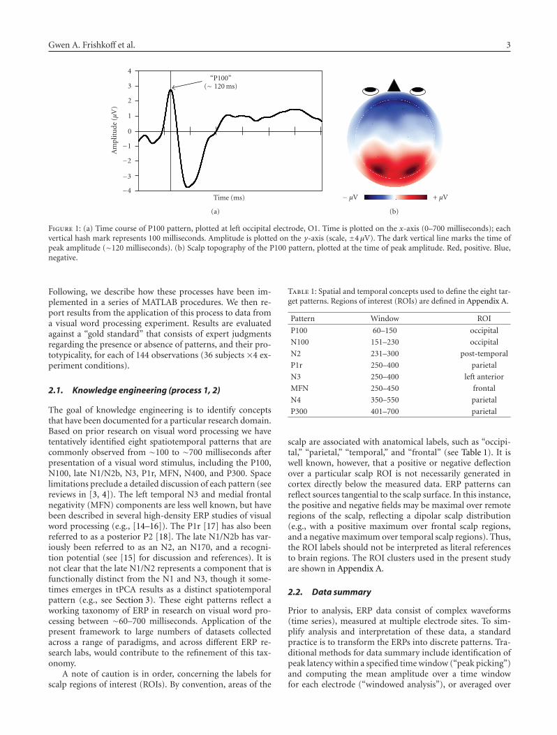
At the same time, ERP methods face some importantchallenges. A key challenge is to identify standardized meth-ods for measure generation, as well as objective and reli-able methods for identification and labeling of ERP com-ponents. Traditionally, researchers have characterized ERPcomponents in respect to both physiological (spatial, tem-poral) and functional criteria [8, 9]. Physiological criteria in-clude latency and scalp distribution, or topography. For ex-ample, as illustrated in Figure 1, the visual “P100 compo-nent” is characterized by a positive deflection that peaks at∼100 milliseconds after onset of a visual stimulus (A) and ismaximal over occipital electrodes, reflecting activity in visualcortex (B).

Despite general agreement on criteria for ERP compo-nent identification [9], in practice such patterns can be hardto identify, particularly in individual subjects. This difficultyis due in part to the superposition of patterns generated bymultiple brain regions at each time point [10], leading tocomplex spatial patterns that reflect the mixing of under-lying patterns. Given this complexity, ERP researchers haveadopted a variety of solutions for scalp topographic analysis(e.g., [11, 12]). It can therefore be difficult to compare re-sults from different studies, even when the same experimen-tal stimuli and task are used.

Similarly, researchers use a variety of methods for de-scribing temporal patterns in ERP data [13]. For example,early components, such as the P100, tend to be character-ized by their peak latency, while the time course of later com-ponents, such as the N400 or P300, is typically captured byaveraging over time “windows” (e.g., 300–500 milliseconds).The latency of other components, such as the N400, has beenquantified in a variety of ways. Finally, there is variabilityin how functional information (e.g., subject-, stimulus-, ortask-specific variables) is used in ERP pattern classification.Some patterns, such as the P100, are easily observed as large

deflections in the raw ERP waveforms. Other patterns, suchas the mismatch negativity are more reliably seen in differ-ence measures, calculated by subtracting ERP amplitude inone condition from the ERP amplitude in a contrasting con-dition. This inconsistency may lead to confusion, particularlywhen the same label is used to refer to two different measures,as is often the case.

1.2. Outline of paper

In summary, the complexity of ERP data has led to multi-ple processes for measure generation and pattern classifica-tion that can vary considerably across different experimentparadigms and across research laboratories. Ultimately, thislimits the ability both to replicate prior results and to gener-alize across findings to achieve high-level interpretations ofERP patterns.

In light of these challenges, the goal of this paper isto describe a framework for automated classification andlabeling of ERP patterns. The framework presented herecomprises both top-down (knowledge-driven) and bottom-up (data-driven) methods for ERP pattern analysis, classi-fication, and labeling. Following, we describe this frame-work in detail (Section 2) and present an application to pat-terns in ERP data from a visual word processing paradigm(Section 3). Section 4 describes approaches to system eval-uation. Section 5 describes data mining for refinement ofexpert-driven (top-down) methods. In Section 6, we drawsome general conclusions and discuss extensions of ourframework for representation of patterns in source space,and ontology development to support cross-paradigm,cross-laboratory, and cross-modal integration of results inEM research.

2. PATTERN CLASSIFICATION FRAMEWORK

As illustrated in Figure 2, our framework comprises five mainprocesses.

(i) Knowledge engineering. Known ERP patterns are cata-loged (1). High-level rules and concepts are describedfor each pattern (2).

(ii) Pattern analysis and measure generation. Analysismethods are selected and applied to ERP data (3). Thegoal is transformation of continuous spatiotemporaldata into discrete patterns for labeling. Statistics aregenerated (4) to capture the rules and concepts identi-fied in (2).

(iii) Data mining. Unsupervised clustering (7) and super-vised learning (8) are used to explore how measurescluster, and how these clusters may be used to identifyand label patterns using rules derived independently ofexpert knowledge.

(iv) Operationalization and application of rules. Rules areoperationalized by combining metrics in (4) with priorknowledge (2). Data mining results (7-8) may be usedto validate and refine the rules. Rules are applied todata, using an automated labeling process (6) detailedbelow.

Gwen A. Frishkoff et al. 3

Time (ms)−4

−3

−2

−1

0

1

2

3

4

Am

plit

ude

(μV

)

“P100”(∼ 120 ms)

(a)

+ μV− μV

(b)

Figure 1: (a) Time course of P100 pattern, plotted at left occipital electrode, O1. Time is plotted on the x-axis (0–700 milliseconds); eachvertical hash mark represents 100 milliseconds. Amplitude is plotted on the y-axis (scale, ±4 μV). The dark vertical line marks the time ofpeak amplitude (∼120 milliseconds). (b) Scalp topography of the P100 pattern, plotted at the time of peak amplitude. Red, positive. Blue,negative.

Following, we describe how these processes have been im-plemented in a series of MATLAB procedures. We then re-port results from the application of this process to data froma visual word processing experiment. Results are evaluatedagainst a “gold standard” that consists of expert judgmentsregarding the presence or absence of patterns, and their pro-totypicality, for each of 144 observations (36 subjects ×4 ex-periment conditions).

2.1. Knowledge engineering (process 1, 2)

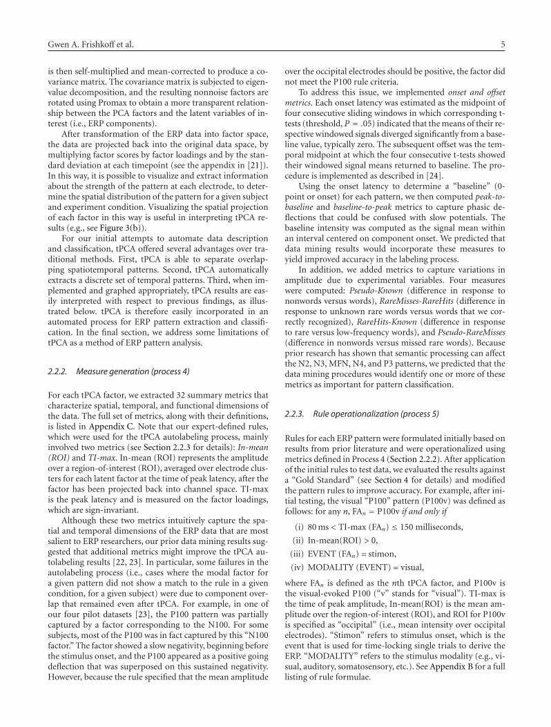
The goal of knowledge engineering is to identify conceptsthat have been documented for a particular research domain.Based on prior research on visual word processing we havetentatively identified eight spatiotemporal patterns that arecommonly observed from ∼100 to ∼700 milliseconds afterpresentation of a visual word stimulus, including the P100,N100, late N1/N2b, N3, P1r, MFN, N400, and P300. Spacelimitations preclude a detailed discussion of each pattern (seereviews in [3, 4]). The left temporal N3 and medial frontalnegativity (MFN) components are less well known, but havebeen described in several high-density ERP studies of visualword processing (e.g., [14–16]). The P1r [17] has also beenreferred to as a posterior P2 [18]. The late N1/N2b has var-iously been referred to as an N2, an N170, and a recogni-tion potential (see [15] for discussion and references). It isnot clear that the late N1/N2 represents a component that isfunctionally distinct from the N1 and N3, though it some-times emerges in tPCA results as a distinct spatiotemporalpattern (e.g., see Section 3). These eight patterns reflect aworking taxonomy of ERP in research on visual word pro-cessing between ∼60–700 milliseconds. Application of thepresent framework to large numbers of datasets collectedacross a range of paradigms, and across different ERP re-search labs, would contribute to the refinement of this tax-onomy.

A note of caution is in order, concerning the labels forscalp regions of interest (ROIs). By convention, areas of the

Table 1: Spatial and temporal concepts used to define the eight tar-get patterns. Regions of interest (ROIs) are defined in Appendix A.

Pattern Window ROI

P100 60–150 occipital

N100 151–230 occipital

N2 231–300 post-temporal

P1r 250–400 parietal

N3 250–400 left anterior

MFN 250–450 frontal

N4 350–550 parietal

P300 401–700 parietal

scalp are associated with anatomical labels, such as “occipi-tal,” “parietal,” “temporal,” and “frontal” (see Table 1). It iswell known, however, that a positive or negative deflectionover a particular scalp ROI is not necessarily generated incortex directly below the measured data. ERP patterns canreflect sources tangential to the scalp surface. In this instance,the positive and negative fields may be maximal over remoteregions of the scalp, reflecting a dipolar scalp distribution(e.g., with a positive maximum over frontal scalp regions,and a negative maximum over temporal scalp regions). Thus,the ROI labels should not be interpreted as literal referencesto brain regions. The ROI clusters used in the present studyare shown in Appendix A.

2.2. Data summary

Prior to analysis, ERP data consist of complex waveforms(time series), measured at multiple electrode sites. To sim-plify analysis and interpretation of these data, a standardpractice is to transform the ERPs into discrete patterns. Tra-ditional methods for data summary include identification ofpeak latency within a specified time window (“peak picking”)and computing the mean amplitude over a time windowfor each electrode (“windowed analysis”), or averaged over


3

4

Pattern analysis & measure generation

ERP component analysis(PCA, peak picking, etc. . .)

Statistical measure generationTime

Peak (ms)

Onset (ms)

Offset (ms)

Etc. . .

Function

Source-language

Stim modality

Subject group

Etc. . .

Space

ROI

Max ch.

Spatial r

Etc. . .

ConceptsTime

Space

FunctionEtc. . .

P100:

∼ 120 msOccipitalpositivity

Stimulus - evoked

1

2

Knowledge engineering

Cataloging knownERP patterns

High-level pattern description

Operationalization & rule application

Operationalization of rules

PTobs = P100 IFF

- 80 ms <= TI- max < 150 ms- ROI = occipital- IN-mean (ROI) > 0- Modality = visual

Component labeling

56

Application of rules(5) to measures (4)

Data mining

Unsupervisedclustering

7 8Supervised learning

System evaluation Revise system

Figure 2: Pattern classification and labeling scheme. Knowledge engineering (processes 1, 2) includes “top-down” specification of ERP con-cepts and rules, formulated by domain experts. Component analysis and measure generation (processes 3, 4) yield summary metrics that areused for pattern classification and labeling. Implementation and operationalization of pattern rules (processes 5, 6) are detailed in Section 2.Data mining (processes 7, 8) includes “bottom-up” or data-driven methods for clustering and discovery of pattern rules (Section 5). Systemevaluation is detailed in Section 4.

electrode clusters (regions of interest—ROIs). An alternativemethod is principal components analysis (PCA), which de-composes the data into “latent” patterns, or factors. The fol-lowing subsection describes this method in detail, and ex-plains the utility of PCA for automated pattern classification.

2.2.1. Temporal PCA methods (process 3)

PCA belongs to a class of factor-analytic procedures, whichuse eigenvalue decomposition to extract linear combinationsof variables (latent “factors”) in such a way as to accountfor patterns of covariance in the data parsimoniously, that is,with the fewest factors. Mathematically, the goal of PCA is totake intercorrelated variables (x1, . . . , xn) and combine themsuch that the tranformed data, the “principal components”(PC), are linear combinations of x, weighted to maximize theamount of variance captured by each eigenvector (vi):

PC1 = v11x1 + v12x2 + · · · + v1nxn. (1)

In this way, the original set of variables (x1, . . . , xn) is “pro-jected” into a new data space, where the dimensions of thisnew space are captured by a small number of latent factors(the eigenvectors).

In ERP data, the variables (x1, . . . , xn) are the microvoltreadings either at consecutive time points (temporal PCA)or at each electrode (spatial PCA). The major source of co-variance isassumed to be the ERP components, characteristicfeatures of the wave form that are spread across multiple timepoints and multiple electrodes. Ideally, each latent factor cor-responds to a separate ERP component, providing a statis-tical decomposition of the brain electrical patterns that aresuperposed in the scalp-recorded data. To achieve this idealfactor-to-pattern mapping, the factors may be “rotated” sothat the variance associated with the original variables (time-points) is redistributed across the factors in such a way thatmaximizes “simple structure,” that is, that achieves a simpleand transparent mapping from variables to factors. (See [19]for a review of PCA and related factor-analytic methods forERP data decomposition.)

In the present application, we used temporal PCA (tPCA)as implemented in the Dien PCA Toolbox [20]. In temporalPCA, the data are organized with the variables correspond-ing to time points and observations corresponding to the dif-ferent waveforms in the dataset. The waveforms vary acrosssubjects, electrodes, and experimental conditions. Thus, sub-ject, spatial, and task variance are collectively responsible forcovariance among the temporal variables. The data matrix


is then self-multiplied and mean-corrected to produce a co-variance matrix. The covariance matrix is subjected to eigen-value decomposition, and the resulting nonnoise factors arerotated using Promax to obtain a more transparent relation-ship between the PCA factors and the latent variables of in-terest (i.e., ERP components).

After transformation of the ERP data into factor space,the data are projected back into the original data space, bymultiplying factor scores by factor loadings and by the stan-dard deviation at each timepoint (see the appendix in [21]).In this way, it is possible to visualize and extract informationabout the strength of the pattern at each electrode, to deter-mine the spatial distribution of the pattern for a given subjectand experiment condition. Visualizing the spatial projectionof each factor in this way is useful in interpreting tPCA re-sults (e.g., see Figure 3(b)).

For our initial attempts to automate data descriptionand classification, tPCA offered several advantages over tra-ditional methods. First, tPCA is able to separate overlap-ping spatiotemporal patterns. Second, tPCA automaticallyextracts a discrete set of temporal patterns. Third, when im-plemented and graphed appropriately, tPCA results are eas-ily interpreted with respect to previous findings, as illus-trated below. tPCA is therefore easily incorporated in anautomated process for ERP pattern extraction and classifi-cation. In the final section, we address some limitations oftPCA as a method of ERP pattern analysis.

2.2.2. Measure generation (process 4)

For each tPCA factor, we extracted 32 summary metrics thatcharacterize spatial, temporal, and functional dimensions ofthe data. The full set of metrics, along with their definitions,is listed in Appendix C. Note that our expert-defined rules,which were used for the tPCA autolabeling process, mainlyinvolved two metrics (see Section 2.2.3 for details): In-mean(ROI) and TI-max. In-mean (ROI) represents the amplitudeover a region-of-interest (ROI), averaged over electrode clus-ters for each latent factor at the time of peak latency, after thefactor has been projected back into channel space. TI-maxis the peak latency and is measured on the factor loadings,which are sign-invariant.

Although these two metrics intuitively capture the spa-tial and temporal dimensions of the ERP data that are mostsalient to ERP researchers, our prior data mining results sug-gested that additional metrics might improve the tPCA au-tolabeling results [22, 23]. In particular, some failures in theautolabeling process (i.e., cases where the modal factor fora given pattern did not show a match to the rule in a givencondition, for a given subject) were due to component over-lap that remained even after tPCA. For example, in one ofour four pilot datasets [23], the P100 pattern was partiallycaptured by a factor corresponding to the N100. For somesubjects, most of the P100 was in fact captured by this “N100factor.” The factor showed a slow negativity, beginning beforethe stimulus onset, and the P100 appeared as a positive goingdeflection that was superposed on this sustained negativity.However, because the rule specified that the mean amplitude

over the occipital electrodes should be positive, the factor didnot meet the P100 rule criteria.

To address this issue, we implemented onset and offsetmetrics. Each onset latency was estimated as the midpoint offour consecutive sliding windows in which corresponding t-tests (threshold, P = .05) indicated that the means of their re-spective windowed signals diverged significantly from a base-line value, typically zero. The subsequent offset was the tem-poral midpoint at which the four consecutive t-tests showedtheir windowed signal means returned to baseline. The pro-cedure is implemented as described in [24].

Using the onset latency to determine a “baseline” (0-point or onset) for each pattern, we then computed peak-to-baseline and baseline-to-peak metrics to capture phasic de-flections that could be confused with slow potentials. Thebaseline intensity was computed as the signal mean withinan interval centered on component onset. We predicted thatdata mining results would incorporate these measures toyield improved accuracy in the labeling process.

In addition, we added metrics to capture variations inamplitude due to experimental variables. Four measureswere computed: Pseudo-Known (difference in response tononwords versus words), RareMisses-RareHits (difference inresponse to unknown rare words versus words that we cor-rectly recognized), RareHits-Known (difference in responseto rare versus low-frequency words), and Pseudo-RareMisses(difference in nonwords versus missed rare words). Becauseprior research has shown that semantic processing can affectthe N2, N3, MFN, N4, and P3 patterns, we predicted that thedata mining procedures would identify one or more of thesemetrics as important for pattern classification.

2.2.3. Rule operationalization (process 5)

Rules for each ERP pattern were formulated initially based onresults from prior literature and were operationalized usingmetrics defined in Process 4 (Section 2.2.2). After applicationof the initial rules to test data, we evaluated the results againsta “Gold Standard” (see Section 4 for details) and modifiedthe pattern rules to improve accuracy. For example, after ini-tial testing, the visual “P100” pattern (P100v) was defined asfollows: for any n, FAn = P100v if and only if

(i) 80 ms < TI-max (FAn) ≤ 150 milliseconds,

(ii) In-mean(ROI) > 0,

(iii) EVENT (FAn) = stimon,

(iv) MODALITY (EVENT) = visual,

where FAn is defined as the nth tPCA factor, and P100v isthe visual-evoked P100 (“v” stands for “visual”). TI-max isthe time of peak amplitude, In-mean(ROI) is the mean am-plitude over the region-of-interest (ROI), and ROI for P100vis specified as “occipital” (i.e., mean intensity over occipitalelectrodes). “Stimon” refers to stimulus onset, which is theevent that is used for time-locking single trials to derive theERP. “MODALITY” refers to the stimulus modality (e.g., vi-sual, auditory, somatosensory, etc.). See Appendix B for a fulllisting of rule formulae.


These rules represent informed hypotheses, based on ex-pert knowledge. As described below (Section 5), bottom-up methods can be used to refine these rules. Further, asthe rules are applied to larger and more diverse sets ofdata, they are likely to undergo additional refinements (seeSection 4.1).

2.2.4. Automated labeling (process 6)

For each condition, subject, and tPCA factor, we used MAT-LAB to compute temporal and spatial metrics on that fac-tor’s contribution to the scalp ERP. The values of the met-rics specified in the expert defined rules were then com-pared to rule-specific thresholds that characterized specificERP components. Thresholds were determined through ex-pert definitions that were formulated and tested as de-scribed in Section 2.2.3). The results of the comparisons wererecorded in a true/false table, and factors meeting all crite-ria were flagged as capturing the specified ERP componentfor that subject and condition. All data were automaticallysaved to Excel spreadsheets organized by rule, condition, andsubject.

2.3. Data mining

As described in Section 2.1, ERP patterns are typically dis-covered through a “manual” process that involves visual in-spection of spatiotemporal patterns and statistical analysis todetermine how the patterns differ across experiment condi-tions. While this method can lead to consensus on the high-level rules and concepts that characterize ERP patterns ina given domain, operationalization of these rules and con-cepts is highly variable across research labs, as described inSection 1. Bottom-up (data-driven) methods can contributeto standardization of rules for classifying known patterns,and possibly to discovery of new patterns, as well. Herewe describe two bottom-up methods, unsupervised learning(i.e., clustering) and supervised learning (i.e., decision treeclassifiers).

2.3.1. Clustering (process 7)

In this study, we used the expectation-maximization (EM) al-gorithm for clustering [25], as implemented in WEKA [26].EM is used to approximate distributions using mixture mod-els. It is a procedure that iterates around the expectation (E)and maximization (M) steps. In the E-step for clustering, thealgorithm calculates the posterior probability, hi j , that a sam-ple j belongs to a cluster Ci:

hi j = P(Ci | Dj

) = p(Dj | θi

)πi

∑ Cm=1p

(Dj | θm

)πm

, (2)

where πi is the weight for the ith mixture component, Dj

is the measurement, and θi is the set of parameters foreach density functions. In the M-step, the EM algorithmsearches for optimal parameters that maximize the sum ofweighted log-likelihood probabilities. EM automatically se-

lects the number of clusters by maximizing the logarithm ofthe likelihood of future data. Observations that belong to thesame pattern type should ideally be assigned to a single clus-ter.

2.3.2. Classification (process 8)

We use a traditional classification technique, called a deci-sion tree learner. Each internal node of a decision tree rep-resents an attribute, and each leaf node represents a class la-bel. We used J48 in WEKA, which is an implementation ofC4.5 algorithm [27]. The input to the decision tree learnerfor the present study consisted of a pattern factor metricsvector of dimension 32, representing the 32 statistical met-rics (Appendix C). Cluster labels were used as classificationlabels. The labeled data set was recursively partitioned intosmall subsets as the tree was being built. If the data instancesin the same subset were assigned to the same label (class),the tree building process was terminated. We then derivedIf-Then rules from the resulting decision tree and comparedthem with expert-generated rules.

3. APPLICATION: VISUAL WORD PROCESSING

The ERP data for this study consisted of 144 observations (36subjects ×4 experiment conditions) that were acquired in alexical decision task (see [28] for details). Participants viewedword and pseudoword stimuli that were presented, one stim-ulus at a time, in the center of a computer monitor and madeword/nonword judgments to each stimulus using their rightindex and middle fingers to depress the “1” and “2” keys on akeyboard (“yes” key counterbalanced across subjects). Stim-uli consisted of 350 words and word-like stimuli, includinglow-frequency words that were familiar to subjects (based onpretesting) and rare words like “nutant” (which were unlikelyto be known by participants). Letters were lower-case Genevablack, 26 dpi, presented foveally on a white screen. Words andnonwords were matched in mean length and orthographicneighborhood [29, 30].

3.1. ERP experiment data

ERP data were recorded using a 128-channel electrode ar-ray, with vertex recording reference [31]. Data were sam-pled at a rate of 250 per second and were amplified with a0.01 Hz highpass filter (time constant∼10 seconds). The rawEEG was segmented into 1500 milliseconds epochs, starting500 milliseconds before onset of the target word. There werefour conditions of interest: correctly classified, low-frequencywords (Known); correctly classified rare words (RareHits),rare words rated as nonwords (RareMisses); and correctlyclassified nonwords (Pseudo).

Segments were marked as bad if they contained ocularartifacts (EOG > 70 μV), or if more than 20% of channelswere bad on a given trial. The artifact-contaminated trialswere excluded from further analysis.

Segmented data were averaged across trials (within sub-jects and within conditions) and digitally filtered with a 30-Hz lowpass filter. After further channel and subject exclusion,


bad (excluded) channels were interpolated. The data re-referenced to the average of the recording sites [32], usinga polar average reference to correct for denser sampling oversuperior, as compared with inferior, scalp locations [33, 34].Data were averaged across individual subjects, and the result-ing “grand-averaged” ERPs were used for inspection of wave-forms and topographic plots.

4. TPCA AUTOLABELING RESULTS

Temporal PCA (tPCA) was used to transform the ERP datainto a set of latent temporal patterns (see Section 2.2.1 fordetails). We extracted the first 15 latent factors from each ofthe four datasets, accounting for approximately 80% of thetotal variance. These 15 tPCA factors were then subjected toa Promax rotation.

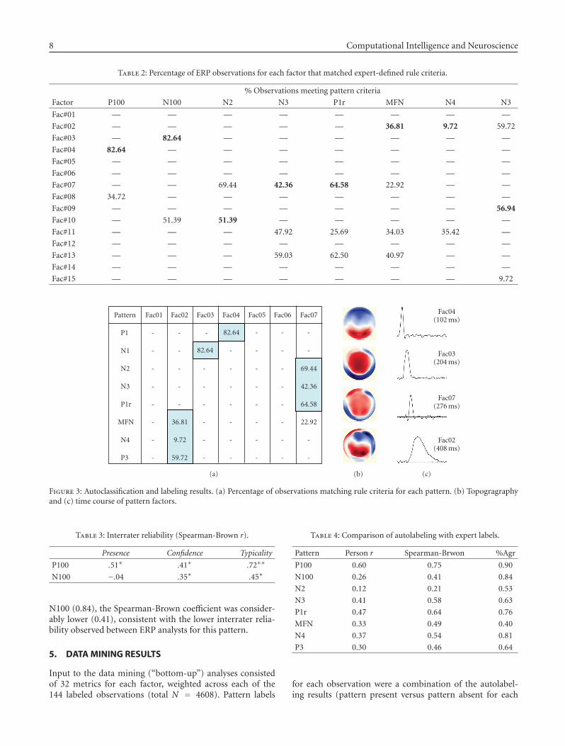
After the tPCA factors were projected back into theoriginal data space (Section 2.2.1), we applied our expert-defined rules to determine the percentage of observationsthat matched each target pattern. Results are shown inTable 2.

We assigned labels to the first 10 factors based on thecorrespondence between the target patterns and the tPCAfactors. Results were as follows: Factor 4 = P100, Factor 3 =N100, Factor = N2, Factor 7 = N3/P1r, Factor 2 = MFN/N4,and Factor 9 = P3. Figure 3 displays the time course and to-pography for these six pattern factors.

Note that many patterns showed splitting across two ormore factors. This may reflect misallocation of pattern vari-ance across the factors (i.e., inaccuracies in the tPCA decom-position), inaccuracies in rule definitions, or both. A com-plementary problem is seen in the case of factors 2, 7, and 10,which show matches to more than one target pattern. Again,this may reflect misallocation of variance. Alternatively, theseresults may suggest a need to refine our pattern descriptions,the rules that are used to identify pattern instances, or both.In either case, these findings point to the need for systematicevaluation of results. Diagnosing potential sources of error isthe first step towards systematic improvements of methods.

4.1. Evaluation of top-down methods

In our framework, top-down methods for pattern classifica-tion are dependent on the accuracy of both the data sum-mary methods and the expert-defined rules. In particular,

(1) data summary methods should yield discrete patternsthat reflect different underlying neuropsychologicalprocesses, or “components;”

(2) rules that are applied to summary metrics should beimplemented in a way that effectively discriminates be-tween separate patterns.

Our initial efforts have led to encouraging classification re-sults, as illustrated above. However, several findings suggestthe need to consider possible misallocation of variance in thedata summary process, and ways of optimizing pattern rules.

4.1.1. Diagnosing misallocation of variance

A well-known critique of PCA methods, including tempo-ral PCA, is that inaccuracies in the decomposition can leadto misallocation of variance ([21, 35]). For example, in ourresults, the left temporal N3 and parietal P1r patterns wereboth assigned to a single factor (cf. [15] for similar results).Recent methods can achieve separation of patterns that havebeen confounded in an initial PCA (see [19] for a discus-sion). A more serious problem is that of the pattern split-ting: well-known patterns like the P100 are expected to mapto a single rule (factor). Indeed, this simple mapping wasobtained in 3 or our 4 pilot datasets [23]. Splitting of theP100 across two factors therefore suggests a possible misal-location of variance in the tPCA. A future challenge will beto develop rigorous methods of diagnosing misallocation ofvariance in the decomposition of ERPs. In the final section,we consider alternatives to tPCA, which may address thisissue.

4.1.2. Comparison with a “gold standard”

The validity of our tPCA autolabeling procedures was as-sessed by comparing autolabeling results with a “gold stan-dard,” which was developed through manual labeling of pat-terns. Two ERP analysts visually inspected the raw ERPs foreach subject and each condition. For each target pattern, theanalysts indicated whether the pattern was present, basedon inspection of temporal data (waveforms, butterfly plots)and spatial data (topography at time of peak activity in pat-tern interval). Analysts also provided confidence ratings andrated the typicality of each pattern instance using a 3-pointscale.

An initial set of ratings on 100 observations (25 subjects×4 conditions) was collected. Raters met to discuss resultsand to calibrate procedures for subsequent ratings. Expertsthen proceeded to label another 116 ERP observations (4 ob-servations were omitted due to a technical error in the datafile). This set of labeled data constituted the “gold standard”for system evaluation.

Interrater reliability for test data was computed for twoof the patterns (P100 and N100) using the Spearman-Brownprophecy coefficient [36]. Results are graphed in Table 3 (“∗”= moderate reliability, “∗∗” = high reliability).

For both patterns, the highest level of reliability was re-flected in the typicality ratings. In addition, reliability wasconsiderably higher for the P100 pattern. Inspection of thedata revealed that the low reliability for N100 “presence”judgments was due to a systematic difference in use of cat-egories: one rater consistently rated as “not present” caseswhere the other rater indicated the pattern was “present” butatypical (“1” on typicality scale).

Accuracy of the autolabeling procedures was definedas the percentage of system labels that matched the gold-standard labels (%Agr; see Table 4). Across the eight patterns,the autolabeling results and expert ratings had an averagedPearson r correlation of +.36. This leads to an effective inter-rater reliability of +.52 as measured by the Spearman-Brownformula. Note that while the %Agr was relatively high for the


Table 2: Percentage of ERP observations for each factor that matched expert-defined rule criteria.

% Observations meeting pattern criteria

Factor P100 N100 N2 N3 P1r MFN N4 N3

Fac#01 — — — — — — — —

Fac#02 — — — — — 36.81 9.72 59.72

Fac#03 — 82.64 — — — — — —

Fac#04 82.64 — — — — — — —

Fac#05 — — — — — — — —

Fac#06 — — — — — — — —

Fac#07 — — 69.44 42.36 64.58 22.92 — —

Fac#08 34.72 — — — — — — —

Fac#09 — — — — — — — 56.94

Fac#10 — 51.39 51.39 — — — — —

Fac#11 — — — 47.92 25.69 34.03 35.42 —

Fac#12 — — — — — — — —

Fac#13 — — — 59.03 62.50 40.97 — —

Fac#14 — — — — — — — —

Fac#15 — — — — — — — 9.72

Pattern Fac01 Fac02 Fac03 Fac04 Fac05 Fac06 Fac07

P1 - - - 82.64 - - -

N1 - - 82.64 - - - -

N2 - - - - - - 69.44

N3 - - - - - - 42.36

P1r - - - - - - 64.58

MFN - 36.81 - - - - 22.92

N4 - 9.72 - - - - -

P3 - 59.72 - - - - -

(a) (b)

Fac04(102 ms)

Fac03(204 ms)

Fac07(276 ms)

Fac02(408 ms)

(c)

Figure 3: Autoclassification and labeling results. (a) Percentage of observations matching rule criteria for each pattern. (b) Topogragraphyand (c) time course of pattern factors.

Table 3: Interrater reliability (Spearman-Brown r).

Presence Confidence Typicality

P100 .51∗ .41∗ .72∗∗

N100 −.04 .35∗ .45∗

N100 (0.84), the Spearman-Brown coefficient was consider-ably lower (0.41), consistent with the lower interrater relia-bility observed between ERP analysts for this pattern.

5. DATA MINING RESULTS

Input to the data mining (“bottom-up”) analyses consistedof 32 metrics for each factor, weighted across each of the144 labeled observations (total N = 4608). Pattern labels

Table 4: Comparison of autolabeling with expert labels.

Pattern Person r Spearman-Brwon %Agr

P100 0.60 0.75 0.90

N100 0.26 0.41 0.84

N2 0.12 0.21 0.53

N3 0.41 0.58 0.63

P1r 0.47 0.64 0.76

MFN 0.33 0.49 0.40

N4 0.37 0.54 0.81

P3 0.30 0.46 0.64

for each observation were a combination of the autolabel-ing results (pattern present versus pattern absent for each


factor, for each observation), combined with typicality rat-ings, as follows. Observations that met the rule criteria (“pat-tern present” according to autolabeling procedures) and wererated as “typical” (rating > “1”) were assigned to one cat-egory label. Observations that either failed to meet patterncriteria (“pattern absent”) or were rated as atypical (“1” onrating scale), or both, were assigned to a second category. Thecombined labels were used to capitalize on the high reliabil-ity and greater sensitivity of the typicality + presence/absenceratings, as compared with the presence/absence labels bythemselves.

For the EM procedures, we set the number of clusters tobe 9 (8 patterns + nonpatterns). We then clustered the 144observations derived from the pattern factors, based on the32 metrics. As shown in Table 5, the assignment of obser-vations to each of the 9 clusters largely agreed with the re-sults from the top-down (autolabeling) procedures (compareTable 2).

Ideally, each cluster will correspond to a unique ERP pat-tern. However, as noted above, inaccuracies in either the datasummary (tPCA) procedures, or the expert rules, or both,can lead to pattern splitting. Thus, it is not surprising thatpatterns in our clustering analysis were occasionally assignedto two or more clusters. For instance, the P100 pattern splitinto two clusters (clusters 4 and 5), consistent with the auto-labeling results (Table 2).

Supervised learning (decision tree) methods were used toderive pattern rules, independently of expert judgments. Ac-cording to the information gain rankings of the 32 attributes,TI-max and In-mean(ROI) were most important, consistentwith our previous results [22]. These findings validate the useof these two metrics in expert-defined rules. Decision treesrevealed the importance of additional spatial metrics, sug-gesting the need for finer-grained characterization of patterntopographies in our rule definitions. In addition, differencemeasures (Pseudo-RareMisses and RareMisses-RareHits) werehighly ranked for certain patterns (the N2 and P300, resp.),suggesting that functional metrics may be useful for classifi-cation of certain target patterns.

6. CONCLUSION

The goal of this study was to define high-level rules andconcepts for ERP components in a particular domain (vi-sual word recognition) and to design, evaluate, and optimizean automated data processing and labeling stream that im-plements these rules and concepts. By combining rule def-initions based on expert knowledge (top-down approach)with rule definitions that are generated through data mining(bottom-up approach), we predicted that our system wouldachieve higher accuracy than a system based on either ap-proach in isolation. Results suggest that the combinationof top-down and bottom-up methods is indeed synergistic:while domain knowledge was used effectively to constrain thenumber of clusters in the data mining, decision tree classi-fiers revealed the importance of additional metrics, includingmultiple measures of topography and, for certain patterns,functional metrics that correspond to experiment manipula-tions.

Ongoing work is focused on the following goals:

(i) refinement of procedures for expert labeling of pat-terns in the “raw” (untransformed) ERP data;

(ii) testing of alternative data summary and autolabelingmethods;

(iii) modification of rules and concepts, based on integra-tion of bottom-up and top-down classification meth-ods.

6.1. Alternative data summary procedures

In the present study, we applied temporal PCA (tPCA) to de-compose ERP data into discrete patterns that are input toour automated component classification and labeling pro-cess. PCA is a useful approach because it is automated, isdata-driven, and has been validated and optimized for de-composition of event-related potentials [21]. At the sametime, as illustrated here, PCA is prone to misallocation ofvariance across the latent factors. Further, differences in thetime course of patterns across subjects and experiment con-ditions are a particular problem for tPCA methods: latency“jitter” can lead to mischaracterization of patterns [7].

For this reason, we are currently testing alternative ap-proaches to ERP component analysis. One approach involvesapplication of sequential (temporo-spatial) PCA. Temporo-spatial PCA is a refinement and extension of temporal PCA(see [12, 19] for details). The factor scores from the tempo-ral PCA, which quantify the extent to which their respectivelatent factors are present in the ERP data, undergo a spatialPCA. The spatial PCA further decomposes the factor scoresinto a second tier of latent factors that capture correlationsbetween channels across subjects and conditions. The latentfactors from the two decompositions are then combined toyield a finer decomposition of the patterns of variance thatare present in the ERP data.

6.1.1. Windowed analysis of ERPs

The second approach is to adopt the traditional methodsof parsing ERP data into discrete temporal “windows” foranalysis. By focusing on temporal windows corresponding toknown ERP patterns, the algorithms we developed for ex-tracting statistics from the tPCA factors can be extended tothe raw ERP, with some modification. While the raw ERPis more complex, with overlapping temporo-spatial patterns,the autolabeling process applied to raw ERPs would corre-spond directly to the expert “gold standard” labeling proce-dure. Furthermore, it would not be subject to one weaknessof tPCA, namely, that the time courses of the factor loadingsare invariant across subjects and conditions.

6.1.2. Microstate analysis

We are also evaluating the use of microstate analysis, an ap-proach to ERP pattern segmentation that was introducedby Lehmann and Skrandies [37]. Microstate analysis is adata parsing technique that partitions the ERP into win-dows based upon characteristics of its evolving topography.


Table 5: EM clustering results (NP: nonpatterns).

0 1 2 3 4 5 6 7 8

P100 0 0 0 0 60 49 0 0 0

N100 1 0 0 0 0 0 7 30 77

N2 104 0 0 0 17 0 0 3 8

N3 5 0 0 0 4 2 2 40 1

P1r 11 0 14 0 14 6 5 51 0

MFN 0 0 0 56 0 9 0 0 0

N4 0 0 0 15 0 1 0 0 0

P3 0 113 0 2 0 0 0 0 0

NP 26 28 22 197 39 16 33 64 20

Consecutive time slices, whose topographies are similar un-der a metric, such as global map similarity, are groupedtogether into a single microstate. This microstate in turncorresponds to a distinct distribution of neuronal activity.Microstate analysis may hold promise for separating ERPcomponents that have minimal temporal overlap. Moreover,this method has been implemented as a fully automatedprocess (see [38] for downloadable software and [39, 40]for discussion of automated segmentation using microstateanalysis).

6.2. Development of neural electromagneticontologies (NEMO)

In previous work [22] we have described progress on the de-sign of a domain ontology mining framework and its ap-plication to EEG data and patterns. This represents a firststep in the development of Neural ElectroMagnetic Ontolo-gies (NEMO). The tools that are developed for the NEMOproject can be used to support data management and patternanalysis within individual research labs. Beyond this goal,ontology-based data sharing can support collaborative re-search that would advance the state of the art in EM brainimaging, by allowing for large-scale metaanalysis and high-level integration of patterns across experiments and imag-ing modalities. Given that researchers currently use differentconcepts to describe temporal and spatial data, ontology de-velopment will require us to develop a common frameworkto support spatial and temporal references.

A practical goal for the NEMO project is to build amerged ERP-ERF ontology for the reading and language do-main. This accomplishment would demonstrate the utility ofontology-based integration of averaged EEG and MEG mea-sures, and make strong contributions to the advancement ofmultimodal neuroinformatics. To accomplish this goal, wehave developed concurrent strategies for representation ofERP and ERF data in sensor space and in source (anatom-ical) space. To link to these ontology databases and to sup-port integration of EM measures with results from otherneuroimaging techniques, we are working to extend our pat-tern classification process to brain-based coordinate systems,through application of source analysis to dense-array EEGand whole-head MEG datasets.

APPENDICES

A. CHANNEL GROUPINGS FOR SPATIAL METRICS(REGIONS OF INTEREST—ROIS)

Left occipital77, 78, 83, 84, 85, 86,89, 90, 91, 92, 95, 96

Right occipital59, 60, 64, 65, 66, 67,69, 70, 71, 72, 74, 75

Leftanterotemporal

27, 28, 33, 34, 35, 39,40, 41, 44, 45, 46, 49,128

Rightanterotemporal

1, 2, 109, 110, 114,115, 116, 117, 120,121, 122, 123, 125

Leftposterotemporal

50. 56, 57, 58, 63, 6465, 69

Rightposterotemporal

91, 96, 97, 100, 101,102, 108

Medial frontal5, 6, 7, 12, 13, 21107, 113, 119

Left parietal7, 31, 32, 37, 38, 42,43, 48, 52, 53, 54, 60,61, 67

Right parietal78, 79, 80, 81, 86, 87,88, 93, 94, 99, 104,105, 106, 107

B. ERP PATTERN RULES HYPOTHESIZED FORVISUAL WORD RECOGNITION

Rule #1 (pattern PT1 = P100)

Let ROI = occipital (average of left and right occipital). For anyn, FAn = PT1 iff

(i) 60 ms < TI-max (FAn) ≤ 150 ms AND(ii) |IN-mean(ROI) | ≥ .4 mV AND

(iii) IN-mean(ROI) > 0.


Table 6

Metric Description

Function

Pseudo-known Difference in mean intensity over ROI at time of peak latency (Nonwords-Words)

RareMisses-RareHits Difference in mean intensity over ROI at time of peak latency (RareMisses-RareHits)

RareHits-Known Difference in mean intensity over ROI at time of peak latency (RareHits-Known)

Pseudo-RareMisses Difference in mean intensity over ROI at time of peak latency (Nonwords-RareMisses)

Intensity

IN-max Maximum intensity (in microvolts) at time of peak latency

IN-max to Baseline Maximum intensity (in microvolts) at time of peak latency with respect to intensity at TI-begin

IN-min Maximum intensity (in microvolts) at time of peak latency

IN-min to Baseline Maximum intensity (in microvolts) at time of peak latency with respect to intensity at TI-begin

SP-max Channel associated with maximum intensity, IN-max

SP-max ROI Channel group (ROI) containing SP-max

SP-min Channel associated with manimum intensity, IN-min

SP-min ROI Channel group (ROI) containing SP-min

Space

IN-mean ROI Mean intensity (in microvolts) at time of peak latency for a specified channel group

IN-LOCC Mean intensity (in microvolts) at time of peak latency for left occipital channel group

IN-ROCC Mean intensity (in microvolts) at time of peak latency for right occipital channel group

IN-LPAR Mean intensity (in microvolts) at time of peak latency for left parietal channel group

IN-RPAR Mean intensity (in microvolts) at time of peak latency for right parietal channel group

IN-LPTEM Mean intensity (in microvolts) at time of peak latency for left posterior temporal channel group

IN-RPTEM Mean intensity (in microvolts) at time of peak latency for right posterior temporal channelgroup

IN-LATEM Mean intensity (in microvolts) at time of peak latency for left anterior temporal channel group

IN-RATEM Mean intensity (in microvolts) at time of peak latency for right anterior temporal channel group

IN-LORB Mean intensity (in microvolts) at time of peak latency for left orbital channel group

IN-RORB Mean intensity (in microvolts) at time of peak latency for right orbital channel group

IN-LFRON Mean intensity (in microvolts) at time of peak latency for left frontal channel group

IN-RFRON Mean intensity (in microvolts) at time of peak latency for right frontal channel group

SP-cor Correlation between factor topography and topography of target pattern

Time

TI-max Latency (in milliseconds) of maximum or minimum amplitude

TI-begin Onset (in milliseconds) of waveform excurstion containing peak intensity

TI-end Conclusion (in milliseconds) of waveform excurstion containing peak intensity

TI-duration Duration (in milliseconds) of pattern, equal to TI-begin minus TI-end

Rule #2 (pattern PT2 = N100)

Let ROI = occipital (average of left and right occipital). For anyn, FAn = PT2 iff

(i) 151 ms < TI-max (FAn) ≤ 229 ms AND

(ii) |IN-mean(ROI)| ≥ .4 mV AND

(iii) IN-mean(ROI) < 0.


Let ROI = occipital-temporal (average of occipital, posteriortemporal). For any n, FAn = PT3 iff





Let ROI = left anterior temporal. For any n, FAn = PT4 iff




Rule #5 (pattern PT5 = P1r)

Let ROI = parietal temporal (average of left parietal, right pari-etal) For any n, FAn = PT5 iff

(i) 250 ms ≥ TI-max (FAn) ≤ 400 ms AND




Rule #6 (pattern PT6 = MFN)

Let ROI = frontocentral (average of left frontocentral, rightfrontocentral) For any n, FAn = PT6 iff

(i) 250 ms < TI-max (FAn) ≤ 450 ms AND(ii) |IN-mean(ROI)| ≥ .4 mV AND




(i) 350 ms < TI-max (FAn) ≤ 550 ms AND(ii) |IN-mean(ROI)| ≥ .4 mV AND


Rule #8 (pattern PT8 = P300)


(i) 401 ms ≥ TI-max (FAn) ≤ 700 ms AND(ii) |IN-mean(ROI)| ≥ .4 mV AND


C. STATISTICAL METRICS

For statistical metrics see Table 6.

ACKNOWLEDGMENTS

This work was supported by a grant to the Oregon Neu-roInformatics Center from the Brain, Biology, and MachineInitiative, Department of Defense, Telemedicine AdvancedTechnology Research Center (TATRC), DAMD17-01-1-0750,“Acquisition of the Oregon ICONIC Grid for Integrated Cog-nitive Neuroscience, Informatics, and Computation,” NSFMajor Research Instrumentation, NSF BCS-0321388.

REFERENCES

[1] W. Klimesch, “Memory processes, brain oscillations and EEGsynchronization,” International Journal of Psychophysiology,vol. 24, no. 1-2, pp. 61–100, 1996.

[2] T.-P. Jung, S. Makeig, M. Westerfield, J. Townsend, E. Courch-esne, and T. J. Sejnowski, “Analysis and visualization of single-trial event-related potentials,” Human Brain Mapping, vol. 14,no. 3, pp. 166–185, 2001.

[3] M. Fabiani, G. Gratton, and M. G. H. Coles, “Event-relatedbrain poten-tials: methods, theory, and applications,” inHandbook of Psychophysiology, J. Cacioppo, L. Tassinary, andG. Berntson, Eds., chapter 3, pp. 53–84, Cambridge UniversityPress, New York, NY, USA, 2000.

[4] A. M. Proverbio and A. Zani, “Electromagnetic manifestationsof mind and brain,” in The Cognitive Electrophysiology of Mindand Brain, A. Zani and A. M. Proverbio, Eds., chapter 2, pp.13–37, Academic Press, New York, NY, USA, 2002.

[5] T. Gasser, J. C. Schuller, and U. S. Gasser, “Correction of mus-cle artefacts in the EEG power spectrum,” Clinical Neurophys-iology, vol. 116, no. 9, pp. 2044–2050, 2005.

[6] O. Hauk, M. H. Davis, M. Ford, F. Pulvermuller, and W. D.Marslen-Wilson, “The time course of visual word recognitionas revealed by linear regression analysis of ERP data,” Neu-roImage, vol. 30, no. 4, pp. 1383–1400, 2006.

[7] K. Spencer, “Averaging, detection, and classification of single-trials ERPs,” in Event-Related Potentials: A Methods Handbook,T. Handy, Ed., pp. 209–228, MIT Press, Cambridge, Mass,USA, 2005.

[8] E. Donchin and E. Heffley, “Multivariate analysis of event-related potential data: a tutorial review,” in MultidisciplinaryPerspectives in Event-Related Brain Potential Research, D. Otto,Ed., pp. 555–572, U.S. Government Printing Office, Washing-ton, DC, USA, 1978.

[9] T. W. Picton, S. Bentin, P. Berg, et al., “Guidelines for usinghuman event-related potentials to study cognition: recordingstandards and publication criteria,” Psychophysiology, vol. 37,no. 2, pp. 127–152, 2000.

[10] P. L. Nunez, Electric Fields of the Brain: The Neurophysics ofEEG, Oxford University Press, New York, NY, USA, 1981.

[11] G. Gratton, M. G. H. Coles, and E. Donchin, “A procedure forusing multi-electrode information in the analysis of compo-nents of the event-related potential: Vector filter,” Psychophys-iology, vol. 26, no. 2, pp. 222–232, 1989.

[12] K. M. Spencer, J. Dien, and E. Donchin, “A componential anal-ysis of the ERP elicited by novel events using a dense electrodearray,” Psychophysiology, vol. 36, no. 3, pp. 409–414, 1999.

[13] T. Handy, “Basic principles of ERP quantification,” in Event-Related Potentials: A Methods Handbook, T. Handy, Ed., pp.33–56, MIT Press, Cambridge, Mass, USA, 2005.

[14] A. C. Nobre and G. McCarthy, “Language-related ERPs: scalpdistributions and modulation by word type and semanticpriming,” Journal of Cognitive Neuroscience, vol. 6, no. 3, pp.233–255, 1994.

[15] J. Dien, G. A. Frishkoff, A. Cerbone, and D. M. Tucker, “Para-metric analysis of event-related potentials in semantic com-prehension: evidence for parallel brain mechanisms,” Cogni-tive Brain Research, vol. 15, no. 2, pp. 137–153, 2003.

[16] G. A. Frishkoff, “Hemispheric differences in strong versusweak semantic priming: evidence from event-related brain po-tentials,” Brain and Language, vol. 100, no. 1, pp. 23–43, 2007.

[17] P. E. Compton, P. Grossenbacher, M. I. Posner, and D. M.Tucker, “A cognitive-anatomical approach to attention in lexi-cal access,” Journal of Cognitive Neuroscience, vol. 3, no. 4, pp.304–312, 1991.

[18] K. Huang, K. Itoh, S. Suwazono, and T. Nakada, “Electrophys-iological correlates of grapheme-phoneme conversion,” Neu-roscience Letters, vol. 366, no. 3, pp. 254–258, 2004.

[19] J. Dien and G. A. Frishkoff, “Introduction to principal com-ponents analysis of event-related potentials,” in Event-RelatedPotentials: A Methods Handbook, T. Handy, Ed., pp. 189–208,MIT Press, Cambridge, Mass, USA, 2005.

[20] J. Dien, “PCA toolbox (version 1.093),” Lawrence, Kan, USA,October 2004.

[21] J. Dien, “Addressing misallocation of variance in principalcomponents analysis of event-related potentials,” Brain Topog-raphy, vol. 11, no. 1, pp. 43–55, 1998.

[22] D. Dou, G. Frishkoff, J. Rong, R. M. Frank, A. Malony, and D.M. Tucker, “Development of NeuroElectroMagnetic Ontolo-gies (NEMO): a framework for mining brainwave ontologies,”in Proceedings of the 13th ACM SIGKDD International Confer-ence on Knowledge Discovery and Data Mining (KDD ’07), pp.270–279, San Jose, Calif, USA, August 2007.

[23] J. Rong, D. Dou, G. A. Frishkoff, R. M. Frank, A. Malony, andD. M. Tucker, “A semi-automatic framework for mining ERP


patterns,” in Proceedings of the 21st International Conference onAdvanced Information Networking and Applications Workshops(AINAW ’07), vol. 1, pp. 329–334, Niagara Falls, Canada, May2007.

[24] A. Rodriguez-Fornells, B. M. Schmitt, M. Kutas, and T. F.Munte, “Electrophysiological estimates of the time course ofsemantic and phonological encoding during listening andnaming,” Neuropsychologia, vol. 40, no. 7, pp. 778–787, 2002.

[25] A. P. Dempster, N. M. Laird, and D. B. Rubin, “Maximum like-lihood from incomplete data via the EM algorithm,” Journal ofthe Royal Statistical Society Series B, vol. 39, no. 1, pp. 1–38,1977.

[26] Weka 3, “Data Mining Software in Java,” http://www.cs.waikato.ac.nz/ml/weka/.

[27] J. Quinlan, C4.5: Programs for Machine Learning, MorganKaufmann, San Mateo, Calif, USA, 1993.

[28] G. A. Frishkoff, C. Perfetti, and C. Westbury, “ERP measuresof partial semantics knowledge: left temporal indices of skilldifferences and lexical quality,” Biological Psychology, in revi-sion.

[29] D. A. Medler and J. R. Binder, “MCWord: an online or-thographic database of the English language,” 2005, http://www.neuro.mcw.edu/mcword/.

[30] M. D. Wilson, “The MRC psycholin-guistic database: machinereadable dictionary,” Behavioural Research Methods, Instru-ments and Computers, vol. 20, no. 1, pp. 6–11, 1988.

[31] Electrical Geodesics (EGI), “Eugene, Oregon,” http://www.egi.com/.

[32] J. Dien, “Issues in the application of the average reference:review, critiques, and recommendations,” Behavior ResearchMethods, Instruments, and Computers, vol. 30, no. 1, pp. 34–43, 1998.

[33] M. Junghofer, T. Elbert, D. M. Tucker, and C. Braun, “Thepolar average reference effect: a bias in estimating the headsurface integral in EEG recording,” Clinical Neurophysiology,vol. 110, no. 6, pp. 1149–1155, 1999.

[34] M. Junghofer, T. Elbert, D. M. Tucker, and B. Rockstroh, “Sta-tistical control of artifacts in dense array EEG/MEG studies,”Psychophysiology, vol. 37, no. 4, pp. 523–532, 2000.

[35] G. McCarthy and C. C. Wood, “Scalp distributions of event-related potentials: an ambiguity associated with analysis ofvariance models,” Electroencephalography and Clinical Neuro-physiology, vol. 62, no. 3, pp. 203–208, 1985.

[36] R. Rosenthal and R. Rosnow, Essentials of Behavioral Research:Methods and Data Analysis, McGraw-Hill, New York, NY,USA, 2nd edition, 1991.

[37] D. Lehmann and W. Skrandies, “Spatial analysis of evoked po-tentials in man—a review,” Progress in Neurobiology, vol. 23,no. 3, pp. 227–250, 1984.

[38] “Cartool software,” Functional Brain Mapping Laboratory,Geneva, Switzerland, http://brainmapping.unige.ch/Cartool.htm.

[39] T. Koenig, K. Kochi, and D. Lehmann, “Event-related electricmicrostates of the brain differ between words with visual andabstract meaning,” Electroencephalography and Clinical Neuro-physiology, vol. 106, no. 6, pp. 535–546, 1998.

[40] T. Koenig and D. Lehmann, “Microstates in language-relatedbrain potential maps show noun-verb differences,” Brain andLanguage, vol. 53, no. 2, pp. 169–182, 1996.

http://www.cs.waikato.ac.nz/ml/weka/

http://www.cs.waikato.ac.nz/ml/weka/

http://www.neuro.mcw.edu/mcword/

http://www.neuro.mcw.edu/mcword/

http://www.egi.com/

http://www.egi.com/

http://brainmapping.unige.ch/Cartool.htm

http://brainmapping.unige.ch/Cartool.htm

Documents

A Framework to Support Automated Classification and Labeling of Brain Electromagnetic Patterns