A framework for good bioﬁlm reactor modeling practice (GBRMP)

1149 © IWA Publishing 2018 Water Science & Technology | 77.5 | 2018

Downloaded from hby UNIVERSITE LAVon 06 August 2018

A framework for good biofilm reactor modeling practice

(GBRMP)

Bruce E. Rittmann, Joshua P. Boltz, Doris Brockmann, Glen T. Daigger,

Eberhard Morgenroth, Kim Helleshøj Sørensen, Imre Takács,

Mark van Loosdrecht and Peter A. Vanrolleghem

ABSTRACT

A researcher or practitioner can employ a biofilm model to gain insight into what controls the

performance of a biofilm process and for optimizing its performance. While a wide range of biofilm-

modeling platforms is available, a good strategy is to choose the simplest model that includes

sufficient components and processes to address the modeling goal. In most cases, a one-

dimensional biofilm model provides the best balance, and good choices can range from hand-

calculation analytical solutions, simple spreadsheets, and numerical-method platforms. What is

missing today is clear guidance on how to apply a biofilm model to obtain accurate and meaningful

results. Here, we present a five-step framework for good biofilm reactor modeling practice (GBRMP).

The first four steps are (1) obtain information on the biofilm reactor system, (2) characterize the

influent, (3) choose the plant and biofilm model, and (4) define the conversion processes. Each step

demands that the model user understands the important components and processes in the system,

one of the main benefits of doing biofilm modeling. The fifth step is to calibrate and validate the

model: System-specific model parameters are adjusted within reasonable ranges so that model

outputs match actual system performance. Calibration is not a simple ‘by the numbers’ process, and

it requires that the modeler follows a logical hierarchy of steps. Calibration requires that the adjusted

parameters remain within realistic ranges and that the calibration process be carried out in an

iterative manner. Once each of steps 1 through 5 is completed satisfactorily, the calibrated model

can be used for its intended purpose, such as optimizing performance, trouble-shooting poor

performance, or gaining deeper understanding of what controls process performance.

doi: 10.2166/wst.2018.021

ttps://iwaponline.com/wst/article-pdf/249089/wst077051149.pdfAL user

Bruce E. RittmannBiodesign Swette Center for EnvironmentalBiotechnology,

Arizona State University,P.O. Box 875701, Tempe, AZ 85287-5701,USA

Joshua P. BoltzVolkert, Inc.,3809 Moffett Road, Mobile, AL 36618,USA

Doris BrockmannINRA Transfert, LBE,Univ. Montpellier, INRA,Narbonne,France

Glen T. DaiggerDept. of Civil and Environmental Engineering,University of Michigan,1351 Beal Ave., Ann Arbor, MI 48109,USA

Eberhard Morgenroth (corresponding author)ETH Zürich,Institute of Environmental Engineering,8093 Zürich,SwitzerlandandEawag,Swiss Federal Institute of Aquatic Science andTechnology,

8600 Dübendorf,SwitzerlandE-mail: [email protected]

Kim Helleshøj SørensenWabag Water Technology Ltd,Bürglistrasse 31, 8401 Winterthur,Switzerland

Imre TakácsDynamita,7 Eoupe, 26110 Nyon,France

Mark van LoosdrechtDept. of Biochemical Engineering,Delft University of Technology,The Netherlands

Peter A. VanrolleghemDépartement de génie civil et de génie des eaux,modelEAU, Université Laval,1065 Av. de la Médecine, Québec, QC G1 V 0A6,Canada

Key words | biofilm, framework, good practice, modeling, reactor

mailto:[email protected]

1150 B. E. Rittmann et al. | Good biofilm reactor modeling practice (GBRMP) Water Science & Technology | 77.5 | 2018

Downloaded by UNIVERSIon 06 Augus

NOTATION

Symbol/abbreviation

from https://TE LAVAL usert 2018

Definition

iwaponline.com/wst/article-pdf/249089/wst077051149.pdf

Dimensionsa

AF
Biofilm surface area L2
BAF
Biological aerated filter
D
Substrate diffusion coefficient in the bulk liquid L2 T�1
DF
Substrate diffusion coefficient in the biofilm L2 T�1
DO
Dissolved oxygen M L�3
IFAS
Integrated fixed-film activated sludge
JF
Substrate flux into the biofilm from the bulk liquid M L�2 T�1
K
Half-maximum-rate concentration M L�3
kattach
Rate coefficient for attachment from the bulk to the biofilm Variableb
kdetach
Rate coefficient for detachment from the biofilm to the bulk Variableb
kLa
Gas-liquid transfer coefficient T�1
LF
Biofilm thickness L
(LLi)
Mass transfer boundary layer thickness (index i: different LL in different stages of the reactor system) L
MBBR
Moving-bed biofilm reactor
MBfR
Membrane biofilm reactor
q̂
Maximum specific rate of substrate utilization Msubstrate Mbiomass�1 T�1
RBC
Rotating biological contactor
S
Substrate concentration in the bulk liquid where substrate is a generic term that can relate to any of therate-limiting compounds such as organic substrate, NH4
þ, NO3�, or O2

Msubstrate L�3

SB
Soluble (readily) biodegradable organic substrate Msubstrate L�3
SF
Substrate concentration inside the biofilm Msubstrate L�3
SLF
Substrate concentration at the outer surface of the biofilm Msubstrate L�3
SOTE
Standard oxygen transfer efficiency –
TSS
Total suspended solids Msolids L�3
UASB
Upflow anaerobic sludge blanket
VSS
Volatile suspended solids Msolids L�3
XF
State variable that quantifies particulate components in a biofilm (biomass per unit biofilm volume).Most biofilm models and simulators consider different types such as heterotrophic biomass (XOHO,F),autotrophic nitrifying biomass (XANO,F), and unbiodegradable particulate biomass (XU,F). The sum ofthese particulate components corresponds to the overall measured XTot,F. Note that the value of thedifferent XF may be constant (as is assumed in Equation (1)) or may vary over the biofilm thickness(Wanner et al. )
Msolids L�3 c

XTot,A
Amount of biomass in the biofilm per unit substratum area (Note: XTot,A¼XTot,F·LF) Msolids L�2
XTot,F
Concentration of biomass in the biofilm (biomass per unit biofilm volume) where biomass is typicallyquantified as VSS, TSS, or COD. In other references XTot,F is sometimes referred to as biofilmbiomass density of biofilm biomass concentration (Note: XTot,F¼XTot,A/LF)
Msolids L�3 c

XU
Particulate unbiodegradable organic matter concentration Msolids L�3
z
Distance dimension perpendicular to the biofilm surface L
α
Ratio of the wastewater to clean water oxygen mass transfer coefficient –
aDimensions are defined according to the SI base quantities L for length, M for mass, T for time. Nomenclature is based on Wanner et al. (2006) and Corominas et al. (2010).bDepends on the type of rate expressions used (e.g., Table 17.4 in Morgenroth 2008).cConcentrations in the biofilm are per unit volume biofilm and not per overall reactor volume. For simple (planar) biofilm geometries the definition of the biofilm volume is straightforward.

For heterogeneous structures the unit biofilm volume considers only the space occupied by particulate components and not the pore space. See also corresponding discussion related to

Figure 2.2(c) in Wanner et al. (2006).



INTRODUCTION

It would not be an exaggeration to say that the developmentand adoption of the International Water Association (IWA)

activated sludge models (ASMs), along with their incorpor-ation into plant-wide modeling protocols, has transformedwastewater-treatment education, research, and practice(Daigger ). Since their introduction (Henze et al. ),these models have become the accepted means of evaluat-ing, designing, and assisting with the operation of waterresources recovery facilities (WRRFs) using the activated

sludge process in its many variations. This is because themodels and associated protocols meet the criteria foruseful application. First, they are based on a combination

of sound science and engineering, and are scalable to pro-vide the level of detail necessary to address real-worldchallenges. Second, the models have kept the complexityas low as possible while encompassing truly important com-

ponents and processes. Third, a strong experience base hasaccumulated to allow their reliable application. Finally,their widespread application provides a common under-

standing and language that facilitate communicationbetween researchers and practitioners, beginning with theinstruction of students learning about biological water

resources recovery.Why do we use models of biological processes? First

and foremost, models are efficient ways of incorporating

known and relevant science, engineering, and practice intoan executable tool. On the one hand, the results of theirproper application can be relied upon for their generalizableaccuracy, in comparison to empirical design criteria, which

are site and situation specific. On the other hand, model fail-ures in specific applications identify areas needing furtherresearch. In this way, the routine and consistent application

of accepted models drives the improvement of fundamentalunderstanding and practice.

Models with firm mechanistic and experiential bases

can be used reliably to establish design and operating cri-teria for WRRFs, resulting in more efficient and effectiveoperation. They also can be used for troubleshooting, i.e.,

identifying the reasons for operating difficulties and necess-ary corrective actions. Likewise, models can be used todetermine the operating limits for existing facilities, alongwith methods to optimize and further increase capacity

and performance.While the ASMs provide these kinds of tools for WRRFs

based on suspended-growth processes, biofilm-based pro-

cesses do not have analogous well-established linkages tobiofilm models. This deficiency cannot be fixed by applying


ASMs to biofilm processes, because of the profound impor-

tance of mass-transport processes in biofilms, along withprocess kinetics (Boltz & Daigger ).

While a plethora of biofilm models exist (Wanner et al.), no consistent and widely used protocol is available toguide the use of biofilm models to design and operate bio-film reactors. This lack of agreed-upon methodology forusing biofilm models has been a barrier to the implemen-

tation of biofilm reactors in WRRFs.What if an agreed-upon means to use biofilm models

were in place? Examples of the practical questions that

could be addressed by a biofilm model include: (1) What isthe achievable flux of ammonium nitrogen (NH4

þ-N), therebyallowing the required size of the biofilm reactor to achieve a

specified effluent concentration to be determined? (2)Why ismy biofilm reactor not performing as well as needed (e.g.,insufficient biochemical oxygen demand (BOD), removal orthe production of nitrate nitrogen, NO2

�-N)? (3) Why does

process performance vary from summer to winter, andwhat can I do about it? (4)What is the biofilm carrier require-ment and associated reactor size for the different types of

biofilm reactors I am considering? (5)Howdo biofilm-carrierfeatures affect important biofilm characteristics, such as sur-face area, detachment rate, and biomass accumulation? It is

easy to see the practical value of a reliable and robust proto-col for modeling biofilm reactors.

In this paper, we present a framework for good biofilm

reactor modeling practice (GBRMP). We first provide a suc-cinct overview of available biofilm models; we conclude thatone-dimensional (1D) models generally are sufficient forengineering practice. We then outline a five-step GBRMP

framework. It is structured along the lines of the widelyused good modeling practices framework for activatedsludge (Rieger et al. ), but with essential differences

related to biofilm reactors.Based on the GBRMP framework, we provide guidance

for selecting the appropriate 1D biofilm model, and we

follow up with simple examples of applying the framework.We conclude with a discussion of the need for model cali-bration and validation when modeling biofilm reactors.

AN OVERVIEW OF BIOFILM MODELS

Biofilm modeling began in the mid-1970s with the seminalworks of Atkinson & Davies (), Williamson & McCarty(), and Harremoes (). The key to each of these early

works was recognizing that the rate of mass transport of sub-strate into the biofilm could limit system performance as



much as the degradation potential by the bacteria inside the

biofilm. Using straightforward 1D reaction and diffusionmodels, these early leaders showed how substrate concen-trations decline with distance into the biofilm. The

bacteria inside the biofilm often experience a much lowersubstrate concentration than those in the bulk liquid or atthe outer surface of the biofilm.

Over four decades have passed since the work of the

pioneers of biofilm modeling. Biofilm modeling has grownin scope, sophistication, and power. Wanner et al. ()published a comprehensive review of biofilm models, and

the reader can find in it excellent details about the structureand use of biofilm models. Here, we provide a succinct over-view of the key features of biofilm models.

Components and processes

A biofilm model is simply a set of mass-balance equationsthat are solved simultaneously. The core of a biofilm model

involves defining the components and processes that are tobe represented by the mass balances. The components aredivided into two broad categories: the microorganisms and

the materials that the microorganisms consume or produce.For modeling biofilms used in wastewater treatment, someimportant sets of components are as follows:

• Heterotrophic bacteria that consume biochemical oxygendemand (BOD) and dissolved oxygen (DO).

• Nitrifying bacteria that consume NH4þ and DO, and pro-

duce NO3�.

• Denitrifying bacteria that consume NO3� and BOD.

For the three sets of components, the microbiologicalprocesses are, respectively, aerobic oxidation of BOD, nitri-fication of NH4

þ, and denitrification of NO3�.

If we want to model all three processes, we need at leastseven mass balances: aerobic heterotrophs, nitrifying bac-teria, denitrifying bacteria, BOD, DO, NH4

þ, and NO3�.

The first three components are solids that form the biofilm.The last four components are soluble materials that canmove through the biofilm. If we are only interested in

aerobic removal of BOD, the mass balance can be simplifiedto aerobic heterotrophs, BOD, and DO. If DO is not limit-ing, then the mass balances can be simplified further toheterotrophs and BOD.

While this seven-component, three-process scenario iswidely applicable, it is only one simple example of systemsthat can be represented by biofilm models. Other com-

ponents and processes that can be incorporated intobiofilmmodels include inert biomass, extracellular polymeric

from https://iwaponline.com/wst/article-pdf/249089/wst077051149.pdfTE LAVAL usert 2018

substances (EPS), refractory organic compounds, anaerobic

ammonium oxidation (anammox) bacteria, sulfur-reducingand -oxidizing bacteria, and organic micro-pollutants.

In addition to microbiological processes, we must

include mass-transport processes, because the substratesneed to move from the bulk liquid to the microorganismsinside the biofilm. The mass-transport processes include dif-fusion or something that can be described by analogy to

diffusion. They are driven by a concentration gradient,which explains why concentration gradients must developin biofilms. Without a concentration gradient, the substrates

cannot get to the bacteria inside the biofilm. Mass transportis important inside the biofilm and also for moving the sub-strates from the bulk liquid to the outside of the biofilm. The

latter is called external mass transfer; it is controlled bythe turbulence in the water moving past the biofilm, andthe result is a concentration gradient between the bulkliquid and the outer surface of the biofilm.

Equations (1) and (2) give a simple example of steady-state mass balances for a single substrate inside a 1D biofilm.Equation (1) shows the balance of diffusion and microbial

utilization inside the biofilm. Equation (2) shows how exter-nal mass transfer provides the same flux of substrate fromthe bulk liquid as into the biofilm.

0 ¼ DFd2SFdz2

� q̂XFSFK þ SF

(1)

JF ¼ DLL

(S� SLF) ¼ DFdSFdz

��z¼0

(2)

S¼ substrate concentration in the bulk liquid, SLF¼ sub-strate concentration at the outer surface of the biofilm, SF¼substrate concentration inside the biofilm, q̂¼ the maximumspecific rate of substrate utilization, K¼ the half-maximum-

rate concentration, XF¼ concentration of active biomass inthe biofilm, DF¼ substrate diffusion coefficient in the bio-film, D¼ substrate diffusion coefficient in the bulk liquid,

JF¼ the substrate flux from the bulk liquid into the biofilm,LL¼ the mass transfer boundary layer thickness, and z¼the distance dimension perpendicular to the biofilm surface.

A detailed discussion of assumptions, boundary conditions,and solutions of Equations (1) and (2) is provided in thereport by Wanner et al. () or in related textbooks

(Rittmann & McCarty ; Morgenroth ).Other important transport processes are the detachment

of biomass from the biofilm and the attachment of sus-pended solids onto the biofilm. Detachment can be

represented in several ways (Wanner et al. ), and it



affects the total amount of metabolically active biomass that

accumulates. If the detachment rate is slower than the netrate of biomass synthesis, the active biomass accumulates,or grows. A faster detachment rate causes the active biomass

to shrink. Attachment of suspended solids also affects thetotal amount of biofilm and how much of it is active biomassversus non-active solids.

Multi-dimensional models

A very important feature of modern biofilm modeling is that

the biofilm can also be represented in two or three dimen-sions, i.e., as 2D and 3D models (Wanner et al. ).Modeling more than one dimension makes it possible to rep-

resent complex changes in the physical morphology ofbiofilms, as well as hydrodynamic interactions between thebiofilm and the water flowing past the biofilm. Multi-dimen-

sional models also allow more sophisticated treatment ofcomplex ecological interactions that occur inside some bio-films. All of these features can be accentuated by recentdevelopments using continuum as well as cellular-automa-

ton and individual-biomass models, along with movie-stylevisualization of the outputs.

While multi-dimensional models add a great deal of

power to biofilm modeling and can offer exceptionalinsights into phenomena that occur in some settings, theydemand heavy computing resources and deep programming

expertise. Thus, 2D and 3D models are used today asresearch tools, but are not realistic for use by engineers tosolve practical problems. Fortunately, a good 1D modelcan address all of the important questions that engineers

need to address. This is true because the dominant processesin all biofilm settings are microbiological reaction and masstransport, which are captured well by a 1D model.

One-dimensional models

Wanner et al. give a comprehensive description of thetypes of 1D models available today. In brief, 1D models canbe broken into three major types. Analytical models make

simplifying assumptions so that Equation (1) can be solvedwith a closed-form analytical equation (Harremoes ;Rittmann & McCarty ). Examples of simplifyingassumptions are using first-order or zero-order kinetics for

the microbiological reaction and neglecting external mass-transfer resistance by assuming that S¼ SLF. Pseudo-analytical models involve algebraic approximations to the

numerical solutions to Equations (1) and (2) (and sometimesalso a mass balance on the biomass) (Rittmann & McCarty


; Morgenroth ). They avoid the assumptions of

analytical solutions and can be implemented with a simplespreadsheet for a limited number of components and pro-cesses (Wanner et al. ). Numerical models use

computer techniques to solve the set of mass-balanceequations. A convenient and often-used tool is AQUASIM(Wanner & Morgenroth ; Wanner et al. ). Numeri-cal solutions require the fewest simplifying assumptions and

can be used to solve systems with many components andprocesses.

Although the following discussion of the GBRMP frame-

work focuses on using 1D numerical models, it isappropriate for any type of biofilm model.

SELECTING A 1D MODEL

With limited understanding of biofilm processes, a novicemodeler may be tempted to ‘play it safe’ by choosing the

most complex biofilm model available. While this strategymight work out well for activated sludge modeling (Grauet al. ), it is not advisable for biofilm reactor modeling.

One reason is that computing time often is a limiting factorfor biofilm reactor modeling, and excess complexityincreases the computational time by orders of magnitude.A second reason is that a complex biofilm model will require

that the user provides many input parameters that are diffi-cult to determine and for which no reliable defaultparameters have been defined. Choosing a too-complex

model will incur many penalties for producing output thatdoes not improve the usefulness for the user.

The following examples provide guidance for deciding

on a suitable model complexity. Figure 1 provides sche-matics of different modeling levels that correspond to theexamples.

Flux of the limiting substrate

As an example, we consider the use of mathematicalmodeling to guide the design of a nitrifying moving-bed bio-

film reactor (MBBR). The reactor can be assumed to becompletely mixed, and the target effluent ammonium con-centrations are low. Based on some simple calculations(e.g., Morgenroth ) the engineer has determined that

the biofilm will be limited by NH4þ and not by DO. Because

this system is limited by a single substrate, a range ofanalytical, pseudo-analytical, and numerical biofilm

models can be applied to calculate the NH4þ

flux and,from that, the necessary surface area of biofilm carrier. If

Figure 1 | Five levels of increasingly complex biofilm models (Levels 1–4) and integrating

modeling results in the overall system design (Level 5). Note that level of

complexity for the modeling of Levels #2 and #3 is identical; the difference is in

the process objectives that in Level #3 consider the benefits resulting from

mass-transport limitations (e.g., different redox zones within the biofilm).



the design also requires the DO flux, it can be estimatedfrom the NH4

þflux based on the known stoichiometry of

NH4þ and O2 utilizations in nitrification (Level #1 in

Figure 1).

Flux of the non-limiting substrate

To design a nitrifying biofilter, the engineer needs to esti-mate NH4

þ and DO fluxes into the biofilm along thelength of the reactor. Due to the relatively high influent

NH4þ concentration, it can be assumed that, in the front

part of the biofilter, the reaction is DO-limited, whereasNH4

þ is rate limiting towards the outlet of the filter. A 1Dnumerical model that takes into account dual substrate

limitations would be appropriate. In addition, the modelneeds to take into account changes in the bulk phase con-centrations along the length of the biofilter, such as by

modeling several biofilm compartments in series (Level#2 in Figure 1).


Competition for substrate and space

A biofilm reactor must oxidize dissolved organic carbon andNH4

þ. Three soluble components need to be considered:

organic substrate (represented as BOD or chemical oxygendemand (COD)), NH4

þ, and their common electron accep-tor, DO. Two unique groups of bacteria must berepresented: faster-growing heterotrophic bacteria oxidizing

the organic substrate and slower-growing autotrophic bac-teria oxidizing NH4

þ. Because performance depends on therelative penetration of the soluble substrates and also on

the spatial distribution of the two groups of bacteria(Wanner & Gujer ), a mathematical model must expli-citly represent the spatial distribution of all soluble

substrates and biomass types. Many simulators, such asAQUASIM, allow this level of detail (Wanner & Morgen-roth ; Boltz et al. ). Depending on the type ofreactor, it may be suitable to assume a constant biofilm

thickness or a constant detachment rate (Level #2 inFigure 1).

Beneficial use of partial penetration

The engineer wants to predict the performance of an aerobic

biofilm reactor in which mass-transport limitations help tocreate unique local ecological niches: aerobic processestowards the outer surface and anoxic or anaerobic processes

towards the core of the biofilm. A numerical model must beused to represent substrate transport and biomass distri-bution within the biofilm. The model needs to describeproduction and consumption of intermediates (e.g., NO3

�

and nitrite (NO2�)) and processes (e.g., denitrification) occur-

ring inside the biofilm based on the intermediates. Thus, thebiofilm must be sub-divided into sufficiently small numerical

segments (or layers) to be able to represent different redoxzones. Most commercial simulators allow for such represen-tations (Level #3 in Figure 1).

Growth, detachment, and attachment

The engineer wants to model the fate of soluble and particu-late organic carbon in an MBBR. While the approach formodeling soluble substrate is well established (e.g.,Equations (1) and (2)), how to describe the fate of particles

within a biofilm reactor is uncertain. Attachment, detach-ment, and transport of particles depends on the biofilm’sphysical structure. Mechanisms of particle attachment,

detachment, and hydrolysis have to be represented, despiteuncertainty. Many biofilm reactor simulators include



approaches to model particle attachment, but the lack of

understanding of the actual mechanisms makes use ofsuch built-in features risky. The modeler often mustimplement novel features based on the best understanding

of the mechanisms affecting attachment and detachment(Level #4 in Figure 1).

Practical reactor implementation

In some cases the performance of a biofilm reactor is notdetermined as much by substrate flux as by physical

phenomena, such as mixing, clogging of the carrier in a bio-filter, and carrier distribution in an MBBR. Mathematicalmodeling can help understand possible biological causes

of some of these problems (e.g., too much biofilm accumu-lation), but many problems are more related to details ofmechanical equipment or complex fluid dynamics. Such fea-tures sometimes cannot be represented by commercial

simulators used for biofilm reactor modeling. In this case,the modeler has to acknowledge that a 1D biofilm modelwill not be sufficient to solve the problem (Level #5 in

Figure 1).

Figure 2 | Overall approach for good biofilm reactor modeling practice.

GBRMP FRAMEWORK

This section introduces a framework for the systematic step-by-

step implementation and calibration of a mathematical modelfor a biofilm reactor (Figure 2). The frameworkwas developedto describe biofilm reactors with suspended support media(e.g., the MBBR and integrated fixed-film activated sludge

(IFAS)), but the underlying principles will be applicable tofixed-bed systems (e.g., biofilters and trickling filters) and toaerobic granular sludge systems. This framework is focused

on basic principles, and it builds on experience frompublishedreports on various aspects of biofilm reactor modeling: struc-tured step-by-step approaches (Vigne et al. ; Vigne et al.; Barry et al. ; Eldyasti et al. ); colloidal organicmatter (Albizuri et al. ; Albizuri et al. ), laboratory-scale MBBRs (Vangsgaard et al. ), predation (Revilla

et al. ), sensitivity and identifiability (Brockmann et al.; Brockmann&Morgenroth ; Boltz et al. ; Brock-mann et al. ), and experimental approaches to determineexternal mass transfer resistance (Nogueira et al. ).

Step 1: obtain information on the biofilm reactor system

Responsible application of a biofilm reactor model requiresa good understanding of the actual biofilm reactor system to


be evaluated. This system-level understanding includes

knowing reactor volumes, mixing conditions (water and bio-film media), available biofilm surface area (AF), microbialprocesses, oxygen transfer, and mechanisms and dynamics

of detachment and biofilm thickness control (Table 1).

Step 2: characterize the influent

Wastewater flow and composition must be quantified interms of average loadings, but also in terms of variabilityof flow and concentration of individual components

(Table 1). In many cases, reactor performance will beimpaired by varying loading. Biofilm reactors typicallyhave a smaller hydraulic retention time (HRT) compared

to activated sludge systems and, therefore, have less hydrau-lic buffering and higher sensitivity to hydraulic variations.

Table 1 | Recommended data requirements for GBRMP

Plant and operational information Wastewater characteristics Reactor and biofilm information

– Flow rates (influent andrecycles)

– Chemical dosing– Water distribution into reactors– Containment structure– Aeration devices and control– Mixing devices and control– Hydrodynamic mixing

conditions– Carrier retention and water

collection systems

– Wastewater composition (total and filteredCOD, readily biodegradable COD (SB),NH4

þ-N, NO2�-N, NO3

�-N, total Kjeldahlnitrogen (TKN) or total nitrogen, PO4

3�-P,total P), VSS, TSS

– Internal recycle flow composition– Daily and seasonal variability

– Mixed liquor suspended solids (MLSS) and mixedliquor volatile suspended solids (MLVSS) ofsuspended biomass

– Amount of biofilm per carrier surface (¼XTot,A)– Biofilm surface area (AF)– Biofilm thickness (LF) and concentration ofbiomass in the biofilm (XTot,F)

– P-content of biomass– Sludge volume index (SVI) of suspended biomass– Bulk liquid DO– Temperature– pH



In principle, wastewater composition can be character-ized following procedures developed for activated sludge

systems (Chapter 5.2 in Rieger et al. ). While the chemi-cal composition (e.g., COD) is independent of whether thewastewater is treated in an activated sludge or a biofilmsystem, the size characterization should reflect retention

and degradation mechanisms (Corominas et al. ). In bio-film systems, soluble compounds are transported into thebiofilm by diffusion, and the corresponding diffusion coeffi-

cient must be quantified. Colloidal and particulatecomponents of COD must be evaluated to determine towhat extent they are transported into the biofilm, attach to

the biofilm, or pass through the system. Thus, the terms sol-uble, colloidal, and particulate refer, on the one hand, toparticle size, but also, on the other hand, to removal mech-anisms. Therefore, retention may be different for activated

sludge and biofilm systems.

Step 3: choose the plant and biofilm model

Flow and retention of water streams, suspended particlesand biomass, and biofilm carriers with biofilm have to be

characterized and implemented in the mathematicalmodel. Note that a reactor may be plug flow for the waterstream and suspended particles, but completely mixed for

biofilm carriers with biofilm in a specific stage or withinthe overall biofilm system (Rittmann ; Boltz et al. ).

The biofilm itself is typically represented using a 1Dlayered model (Wanner et al. ). For many applications,

three to 10 layers are sufficient. Most commercially availablesimulators set the default number of layers to values betweenthree and 10; thus, the user must be alert to increase the

number of layers if needed. For thick and heterogeneous bio-films, more layers may be needed, but increasing the number


of layers significantly increases computational time. Thenumber of layers should be chosen based on an understanding

of the biofilm thickness and the heterogeneity of process con-ditions within the biofilm. For example, if the aerobic zonetowards the surface of the biofilm is in the order of 100 μmthick, the thickness of a single layer must be 100 μm or smal-

ler. A rough rule of thumb is that the number of layers can beestimated by dividing the biofilm thickness by the thickness ofthe smallest process zone in the biofilm.

Biofilms are in many cases mass-transport limited, andmodel predictions are more sensitive to biofilm surfacearea and external mass transfer resistance than to the overall

amount of biomass. In that case, the modeler must either fixa certain biofilm thickness (e.g., based on measurements inthe full-scale reactor) or have the model predict biofilmthickness (e.g., by fixing the value of the detachment and

attachment rate coefficients). Detachment has a particularlystrong influence on biofilm thickness and also on ecologicalniches for slow-growing microorganisms within the biofilm

(Rittmann & Manem ; Rittmann et al. ). Attach-ment of particulate and colloidal components alsoinfluences the availability of organic substrate within the

biofilm and the seeding of the biofilm by suspended biomass.In addition to determining the average biofilm thickness, themodeler also must decide on considerations relating

dynamic changes of biofilm thickness or biofilm detachmentand decide on rate expressions for particle hydrolysis(Janning et al. ; Morgenroth et al. ; Hauduc et al.). Biofilm detachment, attachment, and corresponding

biofilm thickness (average or dynamically varying) canunder some conditions have a significant influence on bio-film reactor performance, but are to-date still not well

understood (Morgenroth & Wilderer ; Morgenroth). It is the responsibility of the model user to understand



the implications of uncertainty in biofilm thickness or

detachment modeling.

Step 4: define the conversion processes

Conversion processes in biofilm reactors – such as BOD andNH4

þ oxidation or denitrification – are similar to processesin activated sludge. Therefore, the existing mathematical

process models developed for activated sludge systems(Henze ) can be adapted for biofilm reactors. A keydifference between activated sludge and biofilm models is

that biofilm models take mass transfer resistances explicitlyinto account, while, for activated sludge systems, the effectof mass transfer resistance into the floc typically is implicitly

modeled by choosing a larger value of the half-maximum-rate concentrations (K). Thus, in biofilm reactor models,the value of the half-maximum-rate concentrations often is

significantly smaller (e.g., 10% of the value in the activatedsludge model) compared to default values in Henze ().When modeling IFAS systems, it will be necessary to usedifferent values for half-maximum-rate concentrations for

suspended biomass and for biomass in biofilms.Different processes may be limiting in biofilm reactors

compared to activated sludge processes. For example, biofilm

reactors more commonly experience NO2� accumulation

compared to activated sludge systems; hence, it may bemore important to implement a two-step nitrification model

when modeling biofilm processes, even if one-step nitrifica-tion works well for activated sludge.

Step 5: calibrate/validate the model

Model calibration adjusts system-specific model parameterswithin reasonable ranges so that relevant model predictions

match actual system performance. Ideally, a first compari-son should be done for steady-state operation and modelpredictions. This is more likely in laboratory and pilot

plants, where influent conditions and reactor operationcan be kept constant for sufficiently long to approachsteady state. Practical biofilm reactors almost always will

have variability in the influent and often also in reactor oper-ation. Achieving steady state in a biofilm simulation can bequite time consuming due to the many interactions amongcomponents and processes. A common mistake, used to

save time, is to start with some random initial conditionsand simply simulate for a few days. This mistake should beavoided, and simulations should be run until all components

reach stable outputs. It can require several months of simu-lated time to reach steady state.


Because biofilm models are complex, model predictions

often are non-linearly related to model input parameters. Fur-thermore, many of the model’s output values are correlatedfor a range of modeling scenarios. While some model par-

ameters (e.g., biofilm thickness) may have no influence onmodel predictions in certain situations (e.g., for thick biofilmsand for low bulk phase substrate concentrations resulting indeep biofilms), the same parameter may have a dominant

influence on model predictions in other settings (e.g. a thinbiofilm with rapid external mass transfer). Thus, parametersensitivities are linked to initial values chosen (Brockmann

et al. ). Regardless of this complexity, it is still possibleto obtain relevant model predictions by following a structuredapproach and by taking into account parameter uncertainty

when interpreting modeling results.The calibration process should followahierarchy bywhich

the most situation-specific parameters are adjusted first, whilethe most well-established parameters are maintained. For

example, if the model is not producing results that correspondto the actual performance, the strategy for adjusting parametersshould follow this sequence. First, the physical parameters –

e.g., flow rates, volumes, and surface areas – should bedouble-checked. If that fails to fix the problem, the secondstep is to re-evaluate the influent characteristics. Third is to

adjust biofilm parameters, such as biomass accumulation andexternal mass-transfer boundary layer thickness. Only if all ofthe preceding adjustments fail should the user resort to adjust-

ing kinetic and, lastly, stoichiometric values.Model calibration usually works best when performed

sequentially following four steps: (1) biomass on carriers,(2) COD or BOD removal, (3) nitrogen removal, and (4)

aeration. Figure 3 lays out a stepwise procedure for cali-bration. The following sub-sections describe typicalprocedures for each step of calibration.

Calibrating biomass on carriers

Determine a realistic biofilm surface area for each reactorstage, and quantify the amount of biofilm biomass in thedifferent reactor stages (calibration step 1a)

In most cases, the supplier of the biofilm support media canprovide the specific surface area for the medium (in m2 bio-film surface per m3 of reactor volume or per m3 of added

media volume). Note that this specific surface area candepend on reactor operation; under certain conditions, theactual value is actually larger than reported by the manufac-

turer (e.g., due to the formation of streamers on the biofilmthat increase the available surface area) or smaller than

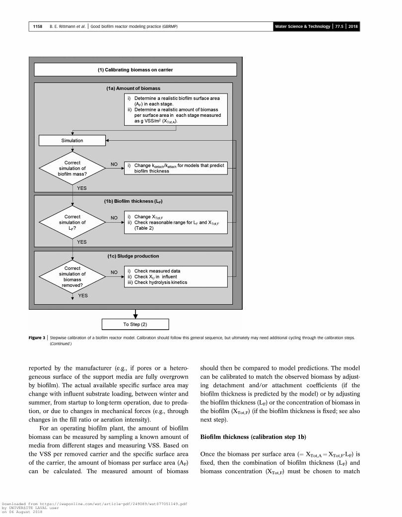
Figure 3 | Stepwise calibration of a biofilm reactor model. Calibration should follow this general sequence, but ultimately may need additional cycling through the calibration steps.

(Continued.)



reported by the manufacturer (e.g., if pores or a hetero-

geneous surface of the support media are fully overgrownby biofilm). The actual available specific surface area maychange with influent substrate loading, between winter andsummer, from startup to long-term operation, due to preda-

tion, or due to changes in mechanical forces (e.g., throughchanges in the fill ratio or aeration intensity).

For an operating biofilm plant, the amount of biofilm

biomass can be measured by sampling a known amount ofmedia from different stages and measuring VSS. Based onthe VSS per removed carrier and the specific surface area

of the carrier, the amount of biomass per surface area (AF)can be calculated. The measured amount of biomass


should then be compared to model predictions. The model

can be calibrated to match the observed biomass by adjust-ing detachment and/or attachment coefficients (if thebiofilm thickness is predicted by the model) or by adjustingthe biofilm thickness (LF) or the concentration of biomass in

the biofilm (XTot,F) (if the biofilm thickness is fixed; see alsonext step).

Biofilm thickness (calibration step 1b)

Once the biomass per surface area (¼ XTot,A¼XTot,F·LF) is

fixed, then the combination of biofilm thickness (LF) andbiomass concentration (XTot,F) must be chosen to match

Figure 3 | Continued.


Downloaded from https://iwaponline.com/wst/article-pdf/249089/wst077051149.pdfby UNIVERSITE LAVAL useron 06 August 2018



this value. Ideally the biofilm thickness should be measured

for the actual biofilm reactor (e.g., microscopically aftersampling a number of carriers, e.g., Bakke & Olsson ).Once the biofilm thickness has been determined, the value

of XTot,F can be directly calculated. For the biofilm thicknessand the biomass concentration, typical values are providedin Table 2.

Sludge production (calibration step 1c)

Sludge production in the actual treatment plant and in

model predictions should be compared. Large deviationsmay mean that sludge production in the treatment plantwas measured incorrectly, particularly since biomass

detachment from the biofilm carriers is a dynamic processrequiring long-term sampling to achieve representativevalues. Another source of deviations between modeling

results and observed reactor operation is an error in thewastewater characterization (e.g., inert particulate organicmatter) or neglecting SB in the effluent. COD mass balan-cing and evaluation of oxygen input (aeration) can be used

to verify the measured sludge production (Rieger et al. ).

COD removal

Degradation of soluble biodegradable COD (calibrationstep 2)

The dominant parameter influencing the degradation ofsoluble biodegradable organic substrate (SB) is the masstransfer boundary layer thickness (LL), if biofilm thickness

and concentration of biomass in the biofilm are fixed.Therefore, measured bulk phase SB concentrations arecompared with model predictions and calibrated by adjust-

ing LL. Typical values for LL are provided in Table 3. Notethat SB should not be confused with the soluble CODmeasured in the reactor, as the soluble COD also includes

the non-biodegradable soluble COD. In activated sludgemodeling, particle characteristics (e.g., size) influenceretention in a clarifier. In modeling a biofilm reactor, par-

ticle characteristics also influence attachment, retention,and potentially transport into the biofilm. Experimentalprocedures are available to differentiate between soluble,colloidal, and particulate COD (e.g., by measuring the fil-

tered COD before or after flocculation. For details ofwastewater characterization and an overview of relatedmethods see Rieger et al. ()).

Note, as biofilm thickness and structure and mixing dueto aeration may vary for different reactor stages, the value of


LL can be significantly different for the different stages. As

LL is influenced by aeration intensity, the value of LL willalso change within a given stage for different air flowrates. One factor that can influence organic substrate degra-

dation is the bulk-phase oxygen concentration, whichshould be measured and included. Another factor influen-cing organic substrate degradation is suspendedheterotrophic biomass (e.g., from detached biomass). Even

without selective retention of suspended biomass in thesystem, the effect of suspended biomass can be significantand should be considered experimentally (e.g., by measuring

the removal rate of biofilm carriers after removing bulkphase biomass) and in the mathematical model.

Nitrogen removal

Nitrification (calibration step 3a)

Nitrification is significantly affected by the presence of hetero-

trophic growth (Wanner & Gujer ), which means thatmodel predictions of nitrification can be realistic only if degra-dation of organic carbon and growth of heterotrophic bacteria

are modeled correctly (calibration step 2). Nitrification in theactual plant should be evaluated based on measurements oforganic nitrogen, NH4

þ, NO2�, and NO3

�. In many practical

cases, only NH4þ and NO3

� are measured, resulting in signifi-cant uncertainty in quantifying the actual extent ofnitrification. Measured nitrification rates and nitrogen com-pounds can be compared with model predictions and, like

in calibration step 2, the rate of ammonia oxidation can beadjusted by adjusting the value of LL in the appropriate stages.

Potential pitfalls that should be considered when model-

ing nitrification are as follows:

• Ammonification of organic nitrogen may be limited in

biofilm reactors due to low HRT.

• Nitrification may be limited by low pH (models usuallymonitor alkalinity as proxy for pH), low phosphorus con-

centrations, or by the presence of inhibitory compounds(check for these limitations both in the model and inthe real plant).

• The number of layers in the mathematical model may

have a significant influence on model predictions as itinfluences how competition between heterotrophic andautotrophic bacteria is modeled.

If in doubt, it may be worth the effort to sample biofilmcarriers and measure nitrification and oxygen uptake rates

in batch experiments after adding ammonium (no organiccarbon) under different operating conditions (variation of

Table 2 | Reasonable parameter values for the concentration of biomass in the biofilm, biofilm thickness, and oxygen transfer to serve as a plausibility check for measured or calibrated values

Carbon oxidation Nitrification

Tertiary denitrificationwithmethanol

Denitrification onmembrane with H2

Concentration of biomass in the biofilm (XTot,F), g VSS/L of biofilm 20–30 40–60 40–60 40–60

Biofilm thickness (LF), μm Trickling filter 500 (Top of trickling filter)100 (Low loaded bottom)

100–200(Top of trickling filter)20–40 (Low loadedbottom)

Like for carbonoxidation, butperhaps withstreamers

RBC 500 (First section)100 (Low loaded lastsection)

100–200 (First section)20–40 (Low loaded lastsection)

BAF (dense media) 100 (before backwashing)40–60 (afterbackwashing)

20–40

BAF (floating media) 100–200 80–120MBBR 500 100–200MBfR (membrane biofilmreactor)

20–80

Continuous washed sandfilter (Dynasand)

10–20No streamers

Fluidized bed reactors 10–20 40–50

DF ¼ 0.8·D

Ratio of the wastewater to clean wateroxygen mass transfer coefficient: α

BAF 1MBBR 0.5–0.9IFAS Like for activated sludge, but media may influence the value

o

1161B.E.

Rittmann

etal. |

Good

biofilm

reactormodeling

practice(GBRM

P)Water

Science

&Tech

nology

|77.5

|2018

Downloaded from https://iwaponline.com/wst/article-pdf/249089/wst077051149.pdfby UNIVERSITE LAVAL useron 06 August 2018

Table 3 | Typical parameter values for flow, carrier sizes, and the external mass transfer boundary layer thickness (LL) to serve as a plausibility check for measured or calibrated values

Type of reactor Liquid velocity in m/h Carrier size in mm LL in μm

Slow sand filter 0.04 0.6 100

Rapid sand filter 5 0.7 20

Trickling filter (low rate) 0.08 40 1,500

Trickling filter (high rate) 1.7 40 20

Submerged biofilm reactor 2–10 2–6 100

MBBR a b 50–180

UASB reactor 1 3 200

Fluidized bed 33 1 20

aNot applicable. bVariable geometries as described in McQuarrie & Boltz (2011); sources: Kissel (1986), Morgenroth (2008).



oxygen set point and/or mixing intensity) to clearly identifywhat is limiting nitrification. Other comments regarding thecalibration of LL from calibration step 2, such as the influ-

ence of air flow rates on LL, should be considered.

Denitrification (calibration step 3b)

Realistic calibration of denitrification relies on reliable

measurements of all nitrogen species, including NO3�, NO2

�,NH4

þ, and organic nitrogen (in particulate organic matterand from biomass synthesis). Modeled denitrification rates

depend on a range of different factors that need to be adjustedbased on understanding of the actual reactor system:

• Availability of competing electron acceptors (e.g., DO).

• Availability of soluble organic carbon (SB) or storage pro-ducts (e.g., PHA) as electron donor and hydrolysis ofcolloidal or particulate organic carbon in the stage

where denitrification occurs.

• External boundary layer thickness (LL) in the stage wheredenitrification occurs. Again, note that the value of LL in

this stage will most likely be larger compared to reactorswith more mixing due to intensive aeration.

• As for nitrification, choosing the right number of layers

for the model is crucial for modeling simultaneous nitrifi-cation and denitrification.

Aeration

Modeling aeration, gas transfer, and oxygen transferbetween stages (calibration step 4)

Biofilm reactors usually are mass-transfer limited, andoxygen often is the limiting factor for carbon oxidation


and nitrification, and can inhibit denitrification. Therefore,overall model predictions will be very sensitive to correctlymodeling the availability of oxygen. Different approaches

are available. If a particular stage in the real plant is oper-ated with a set point for bulk-phase oxygen, then such afixed bulk-phase concentration should also be implemented

in the model. For reactors without aeration the bulk-phaseoxygen concentration should not simply be set to zero, asoxygen may enter from recycles from other reactors in

addition to transfer from the atmosphere. Thus, bulk-phaseoxygen concentrations should always be modeled as astate variable rather than simply assuming a fixed value.

As noted in the previous calibration steps, air flow influ-

ences mixing intensity and indirectly the values of LL in thedifferent stages. That means that it would be desirable todevelop an empirical correlation between oxygen transfer

and gasflow (i.e., kLa and α values) and, in addition, to developan empirical correlation between the gas flow and LL.

Some typical pitfalls and suggestions

• Reactor hydraulics of full-scale plants in general are quite

different from pilot plants or from the original designassumptions made, e.g., an assumed completely mixedreactor may in reality be semi-plug flow.

• The model utilized might not be applicable to the prob-lem: e.g., biological phosphorus removal is taking placein the bulk phase of an IFAS, which requires thatASM2d be used for this aspect.

• The calibration steps outlined above do not always pro-ceed in a linear manner. For example, calibration ofaeration processes may affect earlier steps that involve

DO limitation. Therefore, the entire process may needto proceed in an iterative manner.



CONCLUSIONS AND SUMMARY

A wide range of biofilm models and modeling platforms

are available. A researcher or practitioner can takeadvantage of biofilm modeling to gain insight into whatcontrols the performance of a process and for optimizing

performance. A critical first step is choosing a model thathas the appropriate level of complexity in terms of com-ponents and dimensionality. A good strategy is tochoose the simplest model that includes the necessary

components. In most cases, a 1D biofilm model willwork best, and good choices are available for 1D model-ing. They can range from hand-calculation analytical

solutions, simple spreadsheets, and numerical-methodplatforms.

We present a five-step framework for good practice in

biofilm reactor modeling (GBRMP). The first four stepsare: (1) obtain information on the biofilm reactor system,(2) characterize the influent, (3) choose the plant and bio-

film model, and (4) define the conversion processes. Eachof these steps demands that the model user understandsthe most important components and features of thesystem. Establishing this kind of disciplined thinking is

one of the main benefits of doing biofilm modeling.The fifth step is to calibrate the model: System-specific

model parameters are adjusted within reasonable ranges

so that model outputs match actual system performance.Calibration is not a simple ‘by the numbers’ process,and it requires that the modeler follows a logical hierar-

chy of steps. Calibration requires that the modeler usessound judgment about which parameters are systemspecific and open to calibration. It also requires that theadjusted parameters remain within realistic bounds and

that the calibration process be carried out in an iterativemanner.

Once each of steps 1 through 5 is completed satisfac-

torily, the calibrated model can be used for its intendedpurpose, such as optimizing performance, trouble-shootingpoor performance, or gaining deeper understanding of

what controls process performance.

ACKNOWLEDGEMENTS

The authors acknowledge financial support offered byWorld Water Works and the support of their Chief Technol-

ogy Officer Mr Chandler Johnson. We also acknowledge thesupport of Kruger, North America. Peter Vanrolleghem


holds the Canada Research Chair in Water Quality

Modeling.

REFERENCES

Albizuri, J., van Loosdrecht, M. C. M. & Larrea, L. Extendedmixed-culture biofilms (MCB) model to describe integratedfixed film/activated sludge (IFAS) process behaviour. WaterScience and Technology 60 (12), 3233–3241.

Albizuri, J., Grau, P., Christensson, M. & Larrea, L. Validating the colloid model to optimise the design andoperation of both moving-bed biofilm reactor and integratedfixed-film activated sludge systems. Water Science andTechnology 69 (7), 1552–1557.

Atkinson, B. & Davies, I. J. The overall rate of substrateuptake (reaction) by microbial films. Part I – A biological rateequation. Transactions of the Institution of ChemicalEngineers 52, 248–259.

Bakke, R. & Olsson, P. Q. Biofilm thickness measurements bylight microscopy. Journal of Microbiological Methods 5, 93–98.

Barry, U., Choubert, J. M., Canler, J. P., Heduit, A., Robin, L. &Lessard, P. A calibration protocol of a one-dimensionalmoving bed bioreactor (MBBR) dynamic model for nitrogenremoval. Water Science and Technology 65 (7), 1172–1178.

Boltz, J. P. & Daigger, G. T. Uncertainty in bulk-liquidhydrodynamics and biofilm dynamics creates uncertainties inbiofilm reactor design. Water Science and Technology 61 (2),307–316.

Boltz, J. P., Morgenroth, E. & Sen, D. Mathematicalmodelling of biofilms and biofilm reactors for engineeringdesign. Water Science and Technology 62 (8), 1821–1836.

Boltz, J. P., Morgenroth, E., Brockmann, D., Bott, C., Gellner, W. J.& Vanrolleghem, P. A. Systematic evaluation of biofilmmodels for engineering practice: components and criticalassumptions. Water Science and Technology 64 (4), 930–944.

Boltz, J. P., Johnson, B. R., Takacs, I., Daigger, G. T., Morgenroth,E., Brockmann, D., Kovacs, R., Calhoun, J. M., Choubert,J. M. & Derlon, N. Biofilm carrier migration modeldescribes reactor performance. Water Science andTechnology 75 (12), 2818–2828.

Brockmann, D. & Morgenroth, E. Evaluating operatingconditions for outcompeting nitrite oxidizers andmaintaining partial nitrification in biofilm systems usingbiofilm modeling and Monte Carlo filtering. Water Research44 (6), 1995–2009.

Brockmann, D., Rosenwinkel, K. H. & Morgenroth, E. Practical identifiability of biokinetic parameters of a modeldescribing two-step nitrification in biofilms. Biotechnologyand Bioengineering 101 (3), 497–514.

Brockmann, D., Caylet, A., Escudie, R., Steyer, J. P. & Bernet, N. Biofilm model calibration and microbial diversity studyusing Monte Carlo simulations. Biotechnology andBioengineering 110 (5), 1323–1332.

Corominas, L., Rieger, L., Takacs, I., Ekama, G., Hauduc, H.,Vanrolleghem, P. A., Oehmen, A., Gernaey, K. V., vanLoosdrecht, M. C. M. & Comeau, Y. New framework for

http://dx.doi.org/10.2166/wst.2009.612






http://dx.doi.org/10.1016/0167-7012(86)90005-9

http://dx.doi.org/10.1016/0167-7012(86)90005-9















http://dx.doi.org/10.1016/j.watres.2009.12.010




http://dx.doi.org/10.1002/bit.21932







standardized notation in wastewater treatment modelling.Water Science and Technology 61 (4), 841–857.

Daigger, G. T. A practitioner’s perspective on the uses andfuture developments for wastewater treatment modelling.Water Science and Technology 63 (3), 516–526.

Eldyasti, A., Nakhla, G. & Zhu, J. Development of acalibration protocol and identification of the most sensitiveparameters for the particulate biofilm models used inbiological wastewater treatment. Bioresource Technology111, 111–121.

Grau, P., Copp, J., Vanrolleghem, P. A., Takacs, I. & Ayesa, E. A comparative analysis of different approaches forintegrated WWTP modelling. Water Science and Technology59 (1), 141–147.

Harremoes, P. The significance of pore diffusion to filterdenitrification. Journal Water Pollution Control Federation48 (2), 377–388.

Hauduc, H., Rieger, L., Oehmen, A., van Loosdrecht, M. C. M.,Comeau, Y., Heduit, A., Vanrolleghem, P. A. & Gillot, S. Critical review of activated sludge modeling: state of processknowledge, modeling concepts, and limitations.Biotechnology and Bioengineering 110 (1), 24–46.

Henze, M. The Activated Sludge Models (1, 2, 2d, and 3).IWA Scientific & Technical Report. IWA Publishing,London, UK

Henze, M., Grady Jr., C. P. L., Gujer, W., Marais, G. v.R. &Matsuo, T. Activated Sludge Model No. 1. IAWPRC,London.

Janning, K. F., Le Tallec, X. & Harremoes, P. Hydrolysis oforganic wastewater particles in laboratory scale and pilotscale biofilm reactors under anoxic and aerobic conditions.Water Science and Technology 38 (8–9), 179–188.

Kissel, J. C. Modeling mass-transfer in biological waste-watertreatment processes. Water Science and Technology 18 (6),35–45.

McQuarrie, J. P. & Boltz, J. P. Moving Bed biofilm reactortechnology: process applications, design, and performance.Water Environment Research 83 (6), 560–575.

Morgenroth, E. Detachment – an often overlookedphenomenon in biofilm research and modeling. In: Biofilmsin Wastewater Treatment (S. Wuertz, P. A. Wilderer & P. L.Bishop, eds). IWA Publishing, London, UK, pp. 264–290.

Morgenroth, E. Modelling Biofilms. In: Biological WastewaterTreatment – Principles, Modelling, and Design (M. Henze,M. C. M. van Loosdrecht, G. Ekama & D. Brdjanovic, eds).IWA Publishing, London.

Morgenroth, E. & Wilderer, P. A. Influence of detachmentmechanisms on competition in biofilms. Water Research34 (2), 417–426.

Morgenroth, E., Kommedal, R. & Harremoes, P. Processesand modeling of hydrolysis of particulate organic matter in


aerobic wastewater treatment – a review. Water Science andTechnology 45 (6), 25–40.

Nogueira, B. L., Perez, J., van Loosdrecht, M. C. M., Secchi, A. R.,Dezotti, M. & Biscaia, E. C. Determination of theexternal mass transfer coefficient and influence of mixingintensity in moving bed biofilm reactors for wastewatertreatment. Water Research 80, 90–98.

Revilla, M., Galan, B. & Viguri, J. R. An integratedmathematical model for chemical oxygen demand (COD)removal in moving bed biofilm reactors (MBBR) includingpredation and hydrolysis. Water Research 98, 84–97.

Rieger, L., Gillot, S., Langergraber, G., Ohtsuki, T., Shaw, A.,Takacs, I. & Winkler, S. Guidelines for Using ActivatedSludge Models. IWA Publishing, London, UK.

Rittmann, B. E. Comparative performance of biofilm reactortypes. Biotechnology and Bioengineering 24, 1341–1370.

Rittmann, B. E. & Manem, J. A. Development andexperimental evaluation of a steady-State, multispeciesbiofilm model. Biotechnology and Bioengineering 39 (9),914–922.

Rittmann, B. E. & McCarty, P. L. EnvironmentalBiotechnology: Principles and Applications. McGraw-Hill,New York.

Rittmann, B. E., Stilwell, D. & Ohashi, A. The transient-state,multiple-species biofilm model for biofiltration processes.Water Research 36 (9), 2342–2356.

Vangsgaard, A. K., Mutlu, A. G., Gernaey, K. V., Smets, B. F. &Sin, G. Calibration and validation of a model describingcomplete autotrophic nitrogen removal in a granular SBRsystem. Journal of Chemical Technology and Biotechnologydoi: 10.1002/jctb.4060.

Vigne, E., Choubert, J. M., Canler, J. P., Heduit, A. & Lessard, P. Toward an operational dynamic model for tertiarynitrification by submerged biofiltration. Water Science andTechnology 55 (8–9), 301–308.

Vigne, E., Choubert, J. M., Canler, J. P., Heduit, A., Sorensen, K. &Lessard, P. A biofiltration model for tertiary nitrificationof municipal wastewaters. Water Research 44 (15),4399–4410.

Wanner, O. & Gujer, W. Competition in biofilms. WaterScience and Technology 17 (2–3), 27–44.

Wanner, O. & Morgenroth, E. Biofilm modeling withAQUASIM. Water Science and Technology 49 (11–12),137–144.

Wanner, O., Eberl, H. J., Morgenroth, E., Noguera, D. R.,Picioreanu, C., Rittmann, B. E. & van Loosdrecht, M. C. M. Mathematical Modeling of Biofilms. IWA Publishing,London, UK.

Williamson, K. & McCarty, P. L. Verification studies of thebiofilm model for bacterial substrate utilization. JournalWater Pollution Control Federation 48 (2), 281–296.

First received 9 January 2017; accepted in revised form 16 December 2017. Available online 16 January 2018




http://dx.doi.org/10.1016/j.biortech.2012.02.021








http://dx.doi.org/10.2175/106143010X12851009156286

http://dx.doi.org/10.2175/106143010X12851009156286

http://dx.doi.org/10.1016/S0043-1354(99)00157-8

http://dx.doi.org/10.1016/S0043-1354(99)00157-8














http://dx.doi.org/10.1016/S0043-1354(01)00441-9

http://dx.doi.org/10.1016/S0043-1354(01)00441-9

http://dx.doi.org/10.1002/jctb.4060







Documents

A framework for good bioﬁlm reactor modeling practice (GBRMP)