A FOURTH-ORDER ACCURATE EMBEDDED BOUNDARYappelo/preprints/077223.pdf · A fourth-order accurate embedded boundary method for the scalar wave equation ... problem for both Dirichlet

SIAM J. SCI. COMPUT. c© XXXX Society for Industrial and Applied MathematicsVol. 0, No. 0, pp. 000–000

A FOURTH-ORDER ACCURATE EMBEDDED BOUNDARYMETHOD FOR THE WAVE EQUATION∗

DANIEL APPELO† AND N. ANDERS PETERSON‡

Abstract. A fourth-order accurate embedded boundary method for the scalar wave equationwith Dirichlet or Neumann boundary conditions is described. The method is based on a compactPade-type discretization of spatial derivatives together with a Taylor series method (modified equa-tion) in time. A novel approach for enforcing boundary conditions is introduced which uses interiorboundary points instead of exterior ghost points. This technique removes the small-cell stiffnessproblem for both Dirichlet and Neumann boundary conditions, is more accurate and robust thanprevious methods based on exterior ghost points, and guarantees that the solution is single-valuedwhen slender bodies are treated. Numerical experiments are presented to illustrate the stability andaccuracy of the method as well as its application to problems with complex geometries.

Key words. wave equation, embedded boundary, finite differences

AMS subject classifications. 35L45, 35B35

DOI. 10.1137/09077223X

1. Introduction. Finite difference discretizations with the boundary embed-ded in a Cartesian grid (EB-methods) provide an alternative to body-fitted overset,multiblock, or unstructured grid methods for solving partial differential equations incomplex geometries. The geometry in an EB-method is represented by curves in twodimensions (2D) and surfaces in three dimensions (3D), rather than by surface or volu-metric grids, which significantly reduces storage requirements. For most EB-methods,the geometry need only be accessed while configuring the boundary condition sten-cils, which can be performed during a preprocessing stage. The data-structure forthe boundary condition stencils is simple and all information can be stored in regulararrays. The configuration requires only local operations, making the method well-suited for parallel implementation. Consequently, no costly parallel grid generation isneeded, as the Cartesian grid is trivially generated.

For wave propagation problems, EB-methods generally have small dispersion er-rors due to the perfect regularity of the Cartesian grid. They are also highly efficientin terms of floating point operations and memory use per degree of freedom. Despitethese attractive features relatively few high-order accurate EB-methods for wave equa-tions have been documented in the literature.

This paper presents a fourth-order accurate EB-method for the wave equationbased on compact (Pade-type) finite-difference approximations of spatial derivativescombined with a modified equation approach for the time-discretization. The methodimposes boundary conditions by assigning solution values to boundary points insidethe boundary via interpolation, rather than using extrapolation to assign solutionvalues to ghost points outside the boundary as was done in [9, 10, 11]. This subtle yet

∗Submitted to the journal’s Methods and Algorithms for Scientific Computing section September28, 2009; accepted for publication (in revised form) March 16, 2012; published electronically DATE.

http://www.siam.org/journals/sisc/x-x/77223.html†Department of Mathematics and Statistics, University of New Mexico, Albuquerque, NM, 87131

([email protected]).‡Center for Applied Scientific Computing, Lawrence Livermore National Laboratory, Livermore,

CA 94551 ([email protected]). This author’s work was performed under the auspices of theU.S. Department of Energy by Lawrence Livermore National Laboratory under contract DE-AC52-07NA27344. This is contribution LLNL-JRNL-417163.

A1

A2 DANIEL APPELO AND N. ANDERS PETERSSON

crucial difference improves previous second-order accurate approaches by removingthe small-cell stiffness problem for both Neumann and Dirichlet boundary conditions.Moreover, placing boundary points inside the computational domain allows the solu-tion to be “single-valued” for slender geometries, leading to significant algorithmicsimplifications for complex geometries. A third advantage of placing boundary pointsinside the computational domain is that the boundary conditions are accounted forvia interpolation rather than extrapolation, yielding smaller errors and better stabil-ity properties. To ensure long-time stability, a small amount of artificial dissipationis added.

EB-methods have been used to successfully solve a variety of problems from elas-ticity [30] to incompressible [24] and compressible flows [23]. While this paper will notreview specific applications, it will mention noteworthy papers on high-order-accurateEB-methods for wave equations. Using the integral evolution formula derived byAlpert, Greengard, and Hagstrom [1], Li and Greengard [16] developed high-order(two to six) discretizations for the constant coefficient wave equation. Li and Green-gard first compute a provisional solution ignoring the boundary conditions, and thensolves an integral equation in order to correct the provisional solution. Another familyof high-order (two to eight) accurate discretizations based on the same integral evolu-tion formula was suggested by Wandzura, Visher, and White in [28, 29]. In this casea solution is first obtained by neglecting the boundary conditions and then correctedby a boundary projection. The discretization of the integral evolution is performed bya least squares fit constrained by order of accuracy requirements. Wandzura, Visher,and White approach the issue of stability in a novel way; if a particular discretizationis not stable, they include more neighboring points until it is.

Lombard and Piraux [17] considers coupled acoustic and elastic waves and derivesinterface- and compatibility-conditions on the solution and its derivatives. Specialdiscretizations near the boundary are generated using a least square procedure. Themethod presented in [17] is second-order accurate, but has been extended to fourth-order in [18].

Lyon and Bruno [19, 20, 4] proposed a framework based on Fourier-continuationand alternating direction methods, and devised high-order accurate discretizations forthe scalar wave equation and the heat equation. Their method uses Fourier series rep-resentations of nonperiodic functions to solve boundary value problems arising in ADIformulations. High-order accuracy in time is achieved by Richardson extrapolation.

The proposed method consists of three distinct building blocks: boundary con-dition enforcement, spatial discretization, and temporal discretization. Each of theseblocks can be modified independently of the others to suit a particular applications.For example, it would be straightforward to handle smoothly variable coefficients ormixed Neumann and Dirichlet boundary conditions. Our method is therefore moreflexible than the methods suggested in Li and Greengard and Wandzura, Visher, andWhite, which both are designed solely for the constant coefficient wave equation, orthe unconditionally stable FC-AD solvers in [19], which assume Dirichlet boundaryconditions.

The reminder of this paper is outlined as follows. Section 2 describes the afore-mentioned method in detail, including the precomputations required to enforce theboundary conditions (section 2.1), the temporal (section 2.2) and spatial discretiza-tions (section 2.3), as well as various artificial dissipation operators included to ensurelong-time stability (section 2.4). In section 3, several numerical experiments illustrat-ing the stability and accuracy of the method are presented. Results are compared to

EMBEDDED BOUNDARY METHOD FOR THE WAVE EQUATION A3

previously published data and applications of the method to complex geometries aregiven. A summary and outline of future work is provided in section 4.

2. Description of the method. We consider the wave equation in a two-dimensional domain (x, y) ∈ Ω in an isotropic medium with a constant speed ofsound (for simplicity set to one)

(2.1)∂2u

∂t2=

∂2u

∂x2+

∂2u

∂y2+ f, (x, y) ∈ Ω, t ≥ 0,

with initial data

(2.2) u(x, y, 0) = g0(x, y),∂u

∂t(x, y, 0) = g1(x, y), (x, y) ∈ Ω,

and boundary conditions of Dirichlet

(2.3) u(x, y, t) = h(i)D (x, y, t), (x, y) ∈ Γl, t ≥ 0, l = 1, . . . , nD,

or Neumann type

(2.4)∂u

∂n(x, y, t) = h

(i)N (x, y, t), (x, y) ∈ Γl, t ≥ 0,

l = nD + 1, . . . , nD + nN = ntot.

The boundary of the simply connected domain Ω is a collection of ntot smoothcurves Γl. For an exterior problem the curves Γl must be augmented by a boundarycondition at infinity or by a nonreflecting boundary condition. For an interior problemone curve encloses the ntot − 1 other curves, as shown in Figure 2.1.

2.1. Precomputations. To find an approximate solution to (2.1)–(2.4) we as-sume, without restriction, that all curves describing the geometry are contained insidea rectangular domain (x, y) ∈ Ω = [0, Lx]× [0, Ly] and cover Ω with the uniform grid(see Figure 2.2)

(xi, yj) = (ih, jh), i = 0, . . . , nx, j = 0, . . . , ny.

. ....................... .................... ................ ............. ........... ......... .............................................

...............

.................

..............

...........................................................

................

.............

.................................... ......... ............

Γ1

. ...................................

............

..............

................

...................

......................

.........................

...................

...............

...............................................

.....................

.........

......

........

........

.

........

........

....

........

........

.......

.

........

........

.

.........

.......

..............

........................ ............ ............. ...............

Γ2

......................

...................

..................

.................

..................

...................

.....................

........................................ ......... ....... .......

.....................

........

......

........

........

.

.

........

........

........

....

........

........

........

.

........

........

......

........

........

...

........

........

........

.....

......................................

.....................

................

...................

Γ3

(a) Exterior problem.

. ....................... .................... ................ ............. ........... ......... .............................................

...............

.................

..............

...........................................................

................

.............

.................................... ......... ............

Γ1

. ...................................

............

..............

................

...................

......................

.........................

...................

...............

...............................................

.....................

.........

......

........

........

.

........

........

....

........

........

.......

.

........

........

.

.........

.......

..............

........................ ............ ............. ...............

Γ2

......................

...................

..................

.................

..................

...................

.....................

........................................ ......... ....... .......

.....................

........

......

........

........

.

.

........

........

........

....

........

........

........

.

........

........

......

........

........

...

........

........

........

.....

......................................

.....................

................

...................

Γ3

. ................................................ ............................................. .......................................... ....................................... .................................... ................................. ............................... ........................................................ . .............................

..................................................

...............................................

............................................

........................................

.....................................

..................................

................................

.............................

...........................

..........................

..................................................................................................................................................................................................................................................................................................................................................................

.............

..........................

........

........

........

....

........

........

........

......

........

........

........

........

.

........

........

........

........

...

........

........

........

........

......

........

........

........

........

........

.

........

........

........

........

........

.....

........

........

........

........

........

........

..............

.................... ...........

Γ4

(b) Interior problem.

Fig. 2.1. Possible setups. Note that the setup (a) must be augmented by boundary conditionsat infinity.


. ....................... .................... ................ ............. ........... ......... .............................................

...............

.................

..............

...........................................................

................

.............

.................................... ......... ............

Γ1

. ...................................

............

..............

................

...................

......................

.........................

...................

...............

...............................................

.....................

.........

......

........

........

.

........

........

....

........

........

.......

.

........

........

.

.........

.......

..............

........................ ............ ............. ...............

Γ2

......................

...................

..................

.................

..................

...................

.....................

........................................ ......... ....... .......

.....................

........

......

........

........

.

.

........

........

........

....

........

........

........

.

........

........

......

........

........

...

........

........

........

.....

......................................

.....................

................

...................

Γ3

. ................................................ ............................................. .......................................... ....................................... .................................... ................................. ............................... ........................................................ . .............................

..................................................

...............................................

............................................

........................................

.....................................

..................................

................................

.............................

...........................

..........................

..................................................................................................................................................................................................................................................................................................................................................................

.............

..........................

........

........

........

....

........

........

........

......

........

........

........

........

.

........

........

........

........

...

........

........

........

........

......

........

........

........

........

........

.

........

........

........

........

........

.....

........

........

........

........

........

........

..............

.................... ...........

Γ4

(a)

� � � � � � � � �

� � � �

� � � � � �

� � � � � � �

� � � � � � �

� � � � � � �

� � � � � � �

� � � � � � �

� � � � � � � �

. ....................... .................... ................ ............. ........... ......... .............................................

...............

.................

..............

...........................................................

................

.............

.................................... ......... ............

Γ1

. ...................................

............

..............

................

...................

......................

.........................

...................

...............

...............................................

.....................

.........

......

........

........

.

........

........

....

........

........

.......

.

........

........

.

.........

.......

..............

........................ ............ ............. ...............

Γ2

......................

...................

..................

.................

..................

...................

.....................

........................................ ......... ....... .......

.....................

........

......

........

........

.

.

........

........

........

....

........

........

........

.

........

........

......

........

........

...

........

........

........

.....

......................................

.....................

................

...................

Γ3

. ................................................ ............................................. .......................................... ....................................... .................................... ................................. ............................... ........................................................ . .............................

..................................................

...............................................

............................................

........................................

.....................................

..................................

................................

.............................

...........................

..........................

..................................................................................................................................................................................................................................................................................................................................................................

.............

..........................

........

........

........

....

........

........

........

......

........

........

........

........

.

........

........

........

........

...

........

........

........

........

......

........

........

........

........

........

.

........

........

........

........

........

.....

........

........

........

........

........

........

..............

.................... ...........

Γ4

(b)

Fig. 2.2. Discretization of the geometry without the mask shown (a) and with the maskshown (b), dots indicate mij = 1.

The grid size h > 0 and the number of grid points are chosen such that xnx = Lx andyny = Ly. We denote a time dependent grid function by uij(t) = u(xi, yj, t). Time isdiscretized on a equidistant grid tn = nk with time-step k > 0, and a time discretegrid function is denoted un

ij = u(xi, yj, tn).The solution to (2.1) is sought only at grid points inside Ω. In a precomputation

step a mask grid function mi,j is set up such that

mi,j =

{1, (xi, yj) ∈ Ω,

0 otherwise.

The mask is particularly easy to set up when the boundary of Ω is defined by theimplicit representation φ(x, y)=0. In this case, mi,j simply follows by the sign ofφ(xi, yj). When the boundary curves have a parametric representation, we start bysetting mi,j = −1 at all grid points to indicate that they are undefined. For anexternal problem, the outer edges of the grid are defined as inside by setting mi,j = 1along the lines i = 0, i = nx, j = 0, and j = ny. Correspondingly, for an internalproblem, mi,j = 0 on the outer edges. The mask is then defined in two stages. Foreach boundary curve Γl, we first identify all grid cells that are intersected by theboundary. The grid points at the corners of these grid cells are then marked as eitherinside or outside of Ω by setting mij to 1 or 0. After this step, each boundary curve Γl

has a closed polygon of grid points with mi,j = 1 just inside of Ω and a correspondingclosed polygon of grid points with mi,j = 0, just outside of Ω. In the interior of Ω,the mask can now be defined by “sweeping” line-by-line, i.e., for each horizontal gridline j = 0, 1, . . . , ny, we start at i = 1 and overwrite any undefined mask valuesaccording to

if mi,j = −1, assign mi,j := mi−1,j , i = 1, 2, . . . , nx.

The same procedure is then repeated for each vertical grid line. An example of amask grid function is shown in Figure 2.2.

Boundary conditions are enforced by assigning values to the grid points on thefringe of the computational domain Ω. These points are denoted boundary points.A boundary point (xp, yq) is distinguished by the following criterion: mp,q = 1 and


mp+1,q + mp−1,q + mp,q+1 + mp,q−1 < 4, i.e., the boundary point is inside Ω, butat least one of its nearest neighbors is outside. The boundary points define x- andy-line segments upon which approximations to the spatial derivatives in (2.1) arecomputed. For example, an x-line segment is defined as the collection of grid points(xp, yq), p = p1, . . . , p2 withmp,q = 1, starting and ending at boundary points, (xp1 , yq)and (xp2 , yq), respectively. The boundary points and the line segments are found byinspecting the mask.

To find approximations to spatial derivatives at all points inside the computationaldomain it is sufficient to know all line segments. However, to also account for boundaryconditions some additional precomputations must be performed to determine thestencil and coefficients in the formula for assigning solution values at each boundarypoint. The procedure for setting up such boundary stencils depends on the type ofboundary conditions and the approach taken to enforce them. For Dirichlet boundaryconditions a one-dimensional line-by-line approach can be used which is described insection 2.1.1. The advantage of this approach is ease of implementation and a slightlysmaller error constant than the more general approach described in section 2.1.2.The latter technique, based on interpolation in the direction normal to the boundary,handles both Dirichlet and Neumann boundary conditions.

2.1.1. Enforcing Dirichlet boundary conditions along grid lines. Let(xi, yj) be a boundary point associated with a boundary Γl where the solution isprescribed. To assign a value to uij we introduce a local one-dimensional coordinatesystem ξ along the grid line in x passing through (xi, yj) (left image of Figure 2.3),and construct an interpolating polynomial

(2.5) Iu(ξ) = uijgij(ξ) +

4∑ν=1

uνgν(ξ).

Here gij(ξ), gν(ξ) are the coefficients in the usual Lagrange polynomial basis. Now,by equating the interpolant evaluated on the boundary with the right-hand side ofthe boundary condition

Iu(ξΓ) = hD(xΓ, yΓ, t),

.

.................................................

.............................................

..........................................

.......................................

....................................

................................

.............................

...........................

.........................

.......................

......................

....................

........

........

..

........

........

.........

........

.................

.................

.................

...................

......................

.........................

............................

...............................

.................................

....................................

.......................................

� � � � �uij u1 u2 u3 u4

Γl

ξij ξ1 ξ2 ξ3 ξ4

ξΓ�

��

�ξ

.

.................................................

.............................................

..........................................

.......................................

....................................

................................

.............................

...........................

.........................

.......................

......................

....................

..................

........

........

.........

........

.................

.................

.................

...................

......................

.........................

............................

...............................

.................................

....................................

.......................................

� � � � �uij u1 u2 u3 u4

ξij ξ1 ξ2 ξ3 ξ4

ξΓ�

��

Γl

�ξ

Fig. 2.3. Enforcing Dirichlet boundary conditions by a line-by-line approach using interiorboundary points (left) or exterior ghost points (right).


we obtain an explicit expression for uij

(2.6) uij =1

gij(ξΓ)

(hD(xΓ, yΓ, t)−

4∑ν=1

uνgν(ξΓ)

).

Note that once the intersection of the boundary, ξΓ, is found (e.g., by using a root-finding algorithm such as the secant method) the numbers gij(ξΓ), gν(ξΓ), ν = 1, . . . , 4,do not depend on time and can be precomputed and stored. Also note that the trunca-tion error of (2.6) is of order O(h5). For convenience of implementation a fifth-orderinterpolant is used throughout this paper. For Dirichlet boundary conditions thisyields a fifth-order accurate boundary stencil but for Neumann boundary conditions,which are based on the derivative of the interpolant (2.5), it yields a fourth-orderaccurate boundary stencil.

The placement of the boundary point is the subtle yet important distinction fromprevious papers [9, 10, 11]. In previous work the ghost point is placed outside thecomputational domain as pictured in the right image of Figure 2.3. This placementhas the disadvantage that the denominator of (2.6),

gij(ξΓ) =ξΓ − ξ1ξij − ξ1

4∏ν=2

ξΓ − ξνξij − ξν

,

may become arbitrarily small when ξΓ is close to ξ1 causing small-cell stiffness in anexplicit time stepping procedure.

In contrast, for the approach suggested above, ξΓ ≤ ξij < ξ1 = ξij + h, and thus

|ξΓ − ξ1| ≥ |ξij − ξ1| = h,

so gij(ξΓ) is always bounded away from zero. This separation is an immediate con-sequence of using a Lagrange polynomial basis, i.e., all zeros of gij(ξ) have ξ ≥ ξ1 =ξij + h. Hence, placing the boundary point inside the computational domain removesthe small-cell stiffness problem.

Another advantage with placing the boundary points inside the computationaldomain is that they will be “single-valued” even when the geometry is slender. Thesituation illustrated in Figure 2.4 leads to algorithmic difficulties in that two copies ofthe solution must be stored in ghost points that also are inside Ω. Such special treat-ment leads to more complicated implementations, especially in higher dimensions, sothe algorithmic simplification obtained by using “single-valued” boundary points isimportant in practical applications.

.

...............................

............................

.........................

......................

...................

................

....................... ........ ....... ....... ........

.......................

................

...................

......................

.........................

............................

...............................

� � � �uij u1 u2 u3

.

........

.......................

............................

.........................

......................

...................

................

....................... ........ ....... ....... ........

.......................

................

...................

......................

.........................

............................

...............................

� � � � �uij u1 u2 u3 u4

Fig. 2.4. An advantage with placing the boundary points inside the computational domain isthat they will be “single-valued” even when the geometry is slender. When the boundary pointsare placed outside the computational domain the situation to the right can occur. To the right thesolution is “multivalued” and the values uij and u1 are both interior and boundary points.


Finally, when the boundary points are placed inside the computational domainthe formula (2.6) assigns the value to uij by interpolation rather than extrapolation.In general, interpolation is preferred over extrapolation both for reasons of accuracyand numerical stability.

Remark 1. Note that for the line-by-line approach each boundary point can beassigned either from data along a horizontal or vertical line. If the unit boundarynormal has components n = (n1, n2)

T , we use horizontal grid lines if |n1| > |n2|, andvertical grid lines in the opposite situation.

2.1.2. Enforcing the boundary conditions via interpolation in the nor-mal direction. To enforce Neumann or Dirichlet boundary conditions in a boundarypoint (xi, yj), we find the straight line that passes through the boundary point and isnormal to the boundary curve Γl; see Figure 2.5. Along that line a local coordinateξ is introduced. When the angle, θ, between the line and the horizontal grid linepassing through the boundary point is in the interval 0 ≤ θ ≤ π/4, temporary gridvalues, u1, . . . , u4, at the next four intersections with vertical grid lines are introduced.If π/4 ≤ θ ≤ π/2, temporary values are introduced at the corresponding horizontalintersections (the three other quadrants are simply permutations of the first). Thesolution at the temporary grid points is found by interpolating vertical values. Forexample, in the situation depicted in Figure 2.5 the values would be given by

uν =

qh∑q=ql

⎛⎜⎝ qh∏

p�=qp=ql

(νh sin θ − yj+p)

(yj+q − yj+p)

⎞⎟⎠ui+ν j+q.

Here ql and qh are chosen to center the interpolation stencil as well as possible aroundthe intersection point y = yj + νh sin θ, while only including interior grid points inthe interpolation stencil.

....................

.....................

........................

...........................

.............................

................................

...................................

......................................

........................................

...........................................

..............................................

.................................................

...................................................

��

��

�

�

�

�

�

�

�

�

�

�

�

�

�

�

�

�

�

�

�

�

�

uiju1

u2u3

u4

ξΓl

θ ��

............................

Fig. 2.5. Enforcing the boundary conditions by constructing an interpolating polynomial in thenormal direction. First, the values of the solution at the empty circles are used to interpolate (ver-tically) values, uν , ν = 2, . . . , 4, at the solid circles, then an interpolating polynomial is constructedalong ξ. This polynomial is used to enforce the boundary condition as in the line-by-line approach.


Once the values u1, . . . , u4 are known, the formula (2.5) or its derivative withrespect to ξ is used to find uij for Dirichlet

(2.7) uij =1

gij(ξΓ)

(hD(xΓ, yΓ, t)−

4∑ν=1

uνgν(ξΓ)

),

or for Neumann boundary conditions

(2.8) uij =1

g′ij(ξΓ)

(hN (xΓ, yΓ, t)−

4∑ν=1

uνg′ν(ξΓ)

).

As in the line-by-line approach, the construction of gij(ξ) implies that its rootsare well separated from ξΓ and there will be no small-cell stiffness. For Neumannboundary conditions, Rolle’s theorem guarantees that the denominator of (2.8) is alsoalways bounded away from zero.

Remark 2. Temporary values are introduced at intersections between the gridand the normal in the above description but in the computer implementation of theboundary stencil only a list containing the location of the circled grid points and theweights at those points is stored.

2.2. Approximation in time. Having described the precomputations we nowdescribe the inner-loop, starting with the temporal discretization. To get a fourth-order accurate approximation in time we use the modified equation [2, 6, 26] approachbased on the Taylor expansion of u(x, y, t) around the present time tn, where forbrevity we suppress the dependence on x and y,

u(tn+1) ≈ u(tn) +k

1!ut(tn) +

k2

2!utt(tn) +

k3

3!uttt(tn) +

k4

4!utttt(tn),

u(tn−1) ≈ u(tn)− k

1!ut(tn) +

k2

2!utt(tn)− k3

3!uttt(tn) +

k4

4!utttt(tn).

A fourth-order approximation for u(x, y, tn+1) with the local O(k5) truncationerror is obtained by adding the above equations

u(x, y, tn+1) ≈ 2u(x, y, tn)− u(x, y, tn−1) + k2utt(x, y, tn) +k4

12utttt(x, y, tn).

The terms utt(x, y, tn) and utttt(x, y, tn) are replaced by spatial derivatives using thePDE (2.1). In particular, for smooth u satisfying (2.1) the following equality holds:

(2.9) ∂2t utt(x, y, tn) = ∂2

t (Δu(x, y, tn) + f(x, y, tn))

= Δ(Δu(x, y, tn)) + Δf(x, y, tn) + ftt(x, y, tn).

The evaluation of the right-hand side of (2.9) requires finding approximations of var-ious derivatives of u. Derivatives can be approximated by using a compact Padescheme, as described in detail below; however other one-sided alternatives such assummation-by-parts approximations [12] are also possible.

Remark 3. Note that the value of u(x, y,−k) is needed to start the computationand can be obtained by further Taylor expansion and expressed in terms of the initialdata and forcing as

(2.10) u(x, y,−k) ≈ u(x, y, 0)− kut(x, y, 0)

+k2

2!(Δu(x, y, 0) + f(x, y, 0))− k3

3!(Δut(x, y, 0) + ft(x, y, 0)) .


This approximation is sufficiently accurate to achieve a fourth-order accurate approx-imation of the solution. If highly accurate approximations of the gradient of thesolution are needed, the slow-start procedure described in [9] should be used.

2.3. Approximation of spatial derivatives. Equation (2.9) contains bothsecond and fourth derivatives of the solution. The temporal discretization is fourth-order accurate, and to obtain an overall fourth-order accurate method, second deriva-tives must be approximated using a fourth-order accurate method. For simplicityof implementation, we also approximate the fourth derivatives by the same fourth-order accurate technique, even though it is sufficient to approximate these terms tosecond-order accuracy [2, 6, 26].

As mentioned above, the value of the solution is assigned at the boundary pointsof each line segment and no solution values are extrapolated to outside ghost points.Thus, an approximation of the derivatives that use values only on each line segmentmust be used. For this purpose we use the compact (or Pade) method; see Collatz [5]or Lele [14], which we outline now.

For a one-dimensional grid function ui defined on a grid xi = ih, i = 0, . . . , N ,the compact method approximates the second derivative of u(x) by solving a bandedsystem

(2.11) (uxx)i +

p∑j=1

αj((uxx)i+j + (uxx)i−j) =1

h2

(β0u0 +

q∑l=1

βl(ui+l + ui−l)

),

i = 1, 2, . . . , N − 2, N − 1.

The coefficients αj and βl are found by equating the coefficients in front of increasingpowers of h from the Taylor series expansions of u(x) and uxx(x) around xi. Here theclassic fourth-order accurate Pade scheme [5] is used with p = 1, q = 1, and

α1 = 1/10, β0 = −12/5, β1 = 6/5.

The one-sided stencils

(uxx)0 + 11(uxx)1 =1

h2(13u0 − 27u1 + 15u2 − u3) ,

(uxx)N + 11(uxx)N−1 =1

h2(13uN − 27uN−1 + 15uN−2 − uN−3) ,

are used at the boundary points, x0 and xN .Note that the above boundary closures provide only a third-order accurate ap-

proximation of uxx at the boundary points. However, these values are not used bythe time-stepping algorithm, since the boundary points are assigned values to satisfythe boundary conditions at the end of each time-step.

Remark 4. One drawback to compact schemes is that a system of equations hasto be solved along each line segment. The main objection to solving those systems isnot that it is time consuming (in fact, the most time consuming part is assemblingthe right-hand side when vi+1, vi, vi−1 are not contiguous in memory), but ratherthat it is a global operation which complicates efficient parallelization. A commonparallelization strategy for methods that use compact schemes is to transpose theglobal solution each time step. We argue that a better strategy would be to split thesystem of equations (2.11) on several CPUs realizing that the solution of the systemcan be computed approximately in any point by an explicit method to the same-orderof accuracy.


2.4. Artificial dissipation for long time simulations. LetDPxxuij denote the

compact Pade approximation to uxx(xi, yj). Then the above described approximationof (2.1) can be written

(2.12)un+1ij − 2un

ij + un−1ij

k2=(DP

xx +DPyy

)unij + fn

ij +k2

12

(fn+1ij − 2fn

ij + fn−1ij

k2

)

+k2

12

((DP

xxDPxx + 2DP

yyDPxx +DP

yyDPyy

)unij +

(DP

xx +DPyy

)fnij

)∀ {i, j : mij = 1} .

When used together with an embedded boundary, the scheme (2.12) suffers froma weak instability and a small amount of artificial damping must be added to stabilizeit. Here, we explore the use of three different damping terms:

[−d4h3 (D4x +D4y) + d6h

5 (D6x +D6y)− d8h7 (D8x +D8y)

](unij − un−1

ij

k

)(2.13)

that can be added to the right-hand side of (2.12). The damping terms are approx-

imations of ∂2p

∂x2p∂u∂t , p = 2, 3, 4 built from consistent approximations of dp

dxp , denotedby Dpx. The explicit formulas are found in Appendix B, but generally

∂2p

∂x2p

∂u

∂t≈ DT

pxBpDTpx

(unij − un−1

ij

k

).

The effect of artificial damping on the attainable order of accuracy for summation-by-parts discretizations on Cartesian grids was studied for first-order systems in [22,21]. It was found that the truncation error caused by the damping is of order p + 1when the matrix Bp is chosen as the identity matrix. According to the theory in [21]the d4-damping, which uses B2 = diag(0, 1, 1, . . . , 1, 1, 0), should give second-orderaccuracy while the d6- and d8-damping, for which B3 = B4 = I, should give fourth-and fifth-order accuracy.

In section 3 we experimentally study the convergence properties of the proposedmethod together with the different damping terms (denoted d4-, d6-, or d8-damping).Our findings using an EB-method are not entirely consistent with those of [21]. Forexample, we observe that the truncation-order of the damping is different for Dirichletand Neumann boundary conditions. Also, for the d4-damping we observe only second-order convergence when it is used together with Neumann boundary conditions, butthird-order accurate when used together with Dirichlet boundary conditions.

2.5. Time step restrictions due to damping. To illustrate the basic prop-erties of the damping operator (2.13), we study a one-dimensional model problem.In this section we denote a grid function by un

j = u(xj , tn) and assume that unj is

periodic in space. First, consider the second order accurate approximation of theone-dimensional wave equation with wave speed c = const,

(2.14)un+1j − 2un

j + un−1j

k2= c2D+D−un

j − αh3(D+D−)2unj − un−1

j

k,

where D+unj = (un

j+1 − unj )/h and D−un

j = D+unj−1 denote the forwards and back-

wards divided difference operators, respectively. Let un(ω) be the Fourier series


expansion of unj in space. We have

un+1 − 2un + un−1

k2= −4c2

h2sin2

(ωh

2

)un − αh3

(4

h2sin2

(ωh

2

))2un − un−1

k.

A linear difference equation with constant coefficients is solved by the ansatz

(2.15) un = u0κn,

which gives the characteristic equation

(2.16) κ2 − 2(1− 2λ2σ2 − αλ

)κ+ (1− 2αλ) = 0,

where

σ2 = sin2(ωh

2

), λ =

ck

h, α =

8ασ4

c.

It is instructive to first solve (2.16) for α = 0, i.e., without damping term. Wehave

κ = 1− 2λ2σ2 ±√(1 − 2λ2σ2)2 − 1, α = 0.

If the discriminant is positive, (1 − 2λ2σ2)2 − 1 > 0, both roots κ1,2 are real. Sinceκ1κ2 = 1, one root has magnitude greater than one and the scheme is unstable. Hencethe discriminant must be negative, which results in complex conjugated roots,

κ1,2 = 1− 2λ2σ2 ± i√1− (1− 2λ2σ2)2, α = 0.

Both roots have unit magnitude, |κ1,2| = 1, so the scheme is stable when the discrim-inant is negative. The time step restriction comes from the latter condition, i.e.,

(2.17) (1− 2λ2σ2)2 < 1, i.e., 4λ2σ2(λ2σ2 − 1) < 0.

Since λ2σ2 > 0 and σ2 ≤ 1, the inequality (2.17) is satisfied for all ω if and only if

λ2 =c2k2

h2< 1, i.e, k <

h

c, α = 0,

which is the expected CFL condition for explicit time stepping.When α �= 0, the discriminant of the characteristic equation (2.16) is negative if

(1 − 2λ2σ2 − αλ)2 − (1− 2αλ) < 0, i.e., 4λ2σ2

(1− αλ− λ2σ2 − α2

4σ2

)> 0.

The discriminant becomes zero when

λ2 +α

σ2λ−

(1

σ2− α

4σ4

)= 0, i.e., λ = − α

2σ2± 1

|σ| .

Since λ > 0 by definition, the condition for a negative discriminant becomes

λ =ck

h<

1

|σ|(1− α

2|σ|)

=1

|σ|(1− 8|σ|3α

2c

)≤(1− 4α

c

).

We can draw several interesting conclusions from this formula.


1. There is a maximum value of the dissipation coefficient, αmax = c/4, beyondwhich the scheme becomes unstable regardless of how small the time step ismade.

2. For α < αmax, the damping term restricts the stability limit for the time step,i.e., the time step must always smaller than for the scheme without damping.

3. The damping coefficient should be scaled by the velocity,

α = cα1.

The above analysis can easily be generalized to study higher order damping terms,higher order spatial discretizations, and also the predictor-corrector time-stepping toobtain fourth order accuracy in time. However, these generalizations only modifysome of the constants in the above analysis and does not add any additional insightsinto the stability properties of the scheme.

3. Numerical experiments. In this section we present several experimentsdemonstrating the properties of the proposed method, as summarized in Algorithm 1.

Algorithm 1. Fourth-order-accurate embedded boundary method for

the wave equation.

Data: Geometry, grid size h, time-step k, final time tendResult: The solution un

ij at times t = 0, k, . . . , tendbegin

Pre-computations:

Setup mask, mij ;Setup boundary points;Setup line segments;foreach boundary point do

Setup boundary stencil ;endInitial data:

Assign initial data u0ij ;

Assign u−1ij using (2.10);

Time-stepping loop:

for tn = nk, n = 0, . . . , nt doAssign values to un

ij in all boundary points using the boundary stencils;Compute the right-hand side of (2.12) and store in Fn

ij ;Compute the damping terms (2.13) and store in Dn

ij ;

Compute un+1ij = 2un

ij − un−1ij + k2Fn

ij +Dnij ;

Cycle un−1 ← un, un ← un+1;

end

end

Some of the results presented in this section will be compared to results presentedin [10, 11] and it should be noted that the notation here differs slightly from that in[10, 11]. In particular, the integer N as used below, differs by one although the gridsize h is the same as in [10, 11]. Note also that in section 3.1–3.3 we exclusively reporterrors in max-norm, but we report rate of convergence as

rate = log2‖uapprox.(2h)− uexact‖∞‖uapprox.(h)− uexact‖∞ ,


while rate reported in [10, 11] is the fraction of consecutive errors without taking thelogarithm (i.e., 4 here correspond to 16 in [10, 11]).

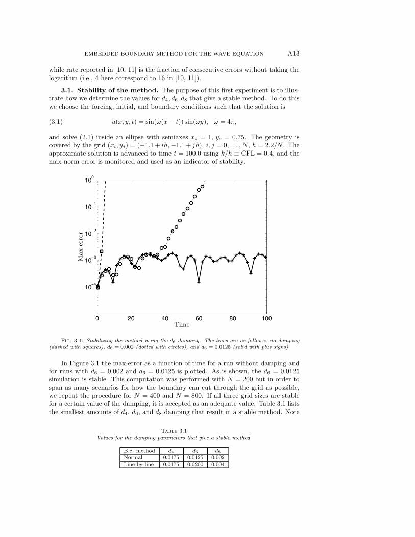
3.1. Stability of the method. The purpose of this first experiment is to illus-trate how we determine the values for d4, d6, d8 that give a stable method. To do thiswe choose the forcing, initial, and boundary conditions such that the solution is

(3.1) u(x, y, t) = sin(ω(x − t)) sin(ωy), ω = 4π,

and solve (2.1) inside an ellipse with semiaxes xs = 1, ys = 0.75. The geometry iscovered by the grid (xi, yj) = (−1.1+ ih,−1.1+ jh), i, j = 0, . . . , N , h = 2.2/N . Theapproximate solution is advanced to time t = 100.0 using k/h ≡ CFL = 0.4, and themax-norm error is monitored and used as an indicator of stability.

0 20 40 60 80 100

10−4

10−3

10−2

10−1

100

Time

Max-error

Fig. 3.1. Stabilizing the method using the d6-damping. The lines are as follows: no damping(dashed with squares), d6 = 0.002 (dotted with circles), and d6 = 0.0125 (solid with plus signs).

In Figure 3.1 the max-error as a function of time for a run without damping andfor runs with d6 = 0.002 and d6 = 0.0125 is plotted. As is shown, the d6 = 0.0125simulation is stable. This computation was performed with N = 200 but in order tospan as many scenarios for how the boundary can cut through the grid as possible,we repeat the procedure for N = 400 and N = 800. If all three grid sizes are stablefor a certain value of the damping, it is accepted as an adequate value. Table 3.1 liststhe smallest amounts of d4, d6, and d8 damping that result in a stable method. Note

Table 3.1

Values for the damping parameters that give a stable method.

B.c. method d4 d6 d8Normal 0.0175 0.0125 0.002Line-by-line 0.0175 0.0200 0.004


that only one of the coefficients are used at a time. To this end, in all computationspresented only one of the coefficients is nonzero. It is possible to use a combinationof them but this would be more computationally expensive. These values have beendetermined by repeating the above experiment, enforcing boundary conditions eitherwith the line-by-line approach or with the normal direction approach on grids withN = 200, 400, 800. The values given for the normal direction approach are suitablefor both Neumann and Dirichlet boundary conditions.

Remark 5. The values presented in Table 3.1 have successfully been used fornumerous geometries and configurations. In our experience, suitable values for thedamping can be determined in a single geometry as long as it is done using sufficientlyfine grids. However, all calculations were performed with unit wave propagation speedand the damping coefficients must be scaled appropriately for other wave speeds asdiscussed in section 2.5.

3.2. Convergence of a trigonometric exact solution. To study the con-vergence properties of the method for different boundary conditions and dampingoptions, we continue to solve the problem described in section 3.1 where the solutionis given by (3.1). Using the values in Table 3.1 for the different damping terms, thesolution is advanced and the max-error monitored to the end time tend = 2 on gridswith N = 200 and 400.

The results for Dirichlet conditions are displayed in Tables 3.2 and 3.3 and theresults for Neumann conditions are displayed in Table 3.4. The output times for theerror are the same as in [10, 11], enabling the comparison with the second-order andthe interior fourth-order-accurate methods therein.

Table 3.2

Convergence of the trigonometric exact solution (3.1) enforcing Dirichlet boundary conditionsline-by-line. The results can be compared to Tables 1 and 2 in [10].

d4 d6 d8t 200 400 Rate 200 400 Rate 200 400 Rate

0.33 1.6(−4) 1.0(−5) 3.96 1.6(−4) 1.0(−5) 3.96 4.6(−5) 1.4(−6) 5.041.98 2.6(−4) 1.5(−5) 4.11 2.6(−4) 1.5(−5) 4.11 4.8(−5) 1.5(−6) 4.972.00 2.7(−4) 1.4(−5) 4.28 2.7(−4) 1.4(−5) 4.28 5.2(−5) 1.6(−6) 5.06

Table 3.3

Convergence of the trigonometric exact solution (3.1) enforcing Dirichlet boundary conditionsby interpolation in the normal direction. The results can be compared to Tables 1 and 2 in [10].


0.33 2.6(−4) 2.6(−5) 3.31 1.3(−4) 8.6(−6) 3.91 8.7(−5) 3.3(−6) 4.711.98 2.8(−4) 2.3(−5) 3.59 2.2(−4) 1.0(−5) 4.43 1.5(−4) 4.3(−6) 5.162.00 2.9(−4) 2.2(−5) 3.71 1.8(−4) 8.9(−6) 4.31 1.5(−4) 4.3(−6) 5.16

Table 3.4

Convergence of the trigonometric exact solution (3.1) with Neumann boundary conditions. Theresults can be compared to Table 2 in [11].


0.33 4.4(−3) 4.0(−4) 3.13 3.5(−3) 2.7(−4) 3.68 3.4(−3) 2.2(−4) 3.941.98 5.5(−3) 7.8(−4) 2.81 4.7(−3) 4.4(−4) 3.41 4.7(−3) 3.0(−4) 3.942.00 6.3(−3) 5.8(−4) 3.43 5.6(−3) 4.1(−4) 3.76 5.4(−3) 3.4(−4) 3.98


Comparing the results with N = 200 for the Dirichlet case with those in Tables 1and 2 in [10], we see that our compact fourth-order-accurate scheme achieves max-errors that are about an order of magnitude smaller than those of the interior fourth-order scheme. Not surprisingly, the improvements compared to the second-orderscheme are even larger.

We find that for both approaches to enforce Dirichlet boundary conditions, thehighest-order damping, d8, gives the most accurate results, followed by the d6-damping.The largest errors are obtained when d4-damping is used. The line-by-line approach isconsistently more accurate than the normal direction approach; this is expected sincethere is only a single interpolation in the line-by-line approach. For both approachesthe convergence rates are higher than expected for the d4- and d8-damping. Whenthe d8-damping is used the dominant error is likely the fifth-order interpolation.

For Neumann boundary conditions the results can be compared to the results inTable 2 in [11]. Here the compact fourth-order accurate scheme yields max-errors thatare approximately five times smaller than those of the interior fourth-order scheme(denoted “predictor-corrector” in [11]).

The observed rates of convergence are lower compared to those observed for theDirichlet case and the d8-damping must be used to get a fourth-order accurate method.However, it is interesting to note that the size of the errors are roughly comparablefor all damping terms.

3.3. Convergence of inwards and outwards traveling waves. In this sec-tion we repeat the experiments with inwards and outwards traveling waves describedin sections 5.2 and 5.3 in [10] and in section 8 in [11]. In all examples the wave equa-tion is solved inside a circle with internal forcing, initial data, and boundary forcingchosen so that the solution becomes a radially propagating wave

(3.2) u(x, y, t) = u(r, t) = φ(r ± t),

where r(x, y)2 = x2 + y2 and

φ(ξ) =1

4

(1 + tanh

ξ − ξ0ε

)(1− tanh

ξ − ξ1ε

).

To be precise the initial data is obtained from (3.2) as is the Dirichlet boundaryconditions. The forcing, f , in (2.1) is f = φtt − φxx − φyy and for the Neumannboundary conditions φr is used (the derivatives of φ can be found, for example, byMaple).

In this section all boundary conditions are enforced via interpolation in the normaldirection. We note that for these short-time simulations no artificial dissipation isrequired, but we still use d6-damping for Dirichlet conditions and d8-damping forNeumann conditions, as we believe they will be needed in many realistic long-timeapplications of the method.

3.3.1. Convergence of an inwards and outwards traveling wave withDirichlet conditions. First, consider convergence of an inwards traveling wave with

u(x, y, t) = φ(r + t), ξ0 = 2.2, ξ1 = 2.4, ε = 0.035,

in a circle |r| ≤ 2 with Dirichlet boundary conditions. The circle is covered by arectangle of size 4.2× 4.2 discretized by a uniform grid with h = 4.2/N .

This problem is more challenging than the trigonometric exact solution as thewave has a much steeper gradient. The wave starts outside the domain and reaches


Table 3.5

Convergence results for an inwards traveling wave with Dirichlet boundary conditions.

CFL = 0.4 CFL = 0.4 CFL = 0.1 CFL =0.1t N = 400 N = 800 Rate N = 400 N = 800 Rate

0.315 8.31(−3) 9.80(−4) 3.08 8.94(−3) 1.16(−3) 2.950.525 8.25(−3) 9.77(−4) 3.08 9.13(−3) 1.15(−3) 2.991.155 8.96(−3) 6.87(−4) 3.71 1.02(−2) 8.26(−4) 3.621.365 9.89(−3) 7.07(−4) 3.81 1.13(−2) 8.72(−4) 3.69

its maximum on the boundary around t ≈ 0.3 and then continues to propagate towardsthe center of the circle.

In Table 3.5 results from simulations using two CFL numbers, CFL = 0.4 andCFL = 0.1, and two discretizations, N = 400 and N = 800, are presented. For thisexperiment the errors are comparable with those presented in [10] (Tables 3 and 4).This supports the argument made in [10] that for certain problems, consisting ofwaves residing mainly in the interior, the interior fourth-order correction can be quiteeffective.

Note that the rates of convergence are lower than four at the earlier times when thewave is entering the domain. We expect that the rates of convergence would approachfour if the grid would be refined further, and that the errors for the compact methodwould be much smaller than those of the interior fourth-order method.

Next we consider the convergence of an outwards traveling wave with

u(x, y, t) = φ(r − t), ξ0 = 0.2, ξ1 = 0.4, ε = 0.035,

in a circle |r| ≤ 1 with Dirichlet boundary conditions. Now the circle is covered by arectangle of size 2.2×2.2 discretized with h = 2.2/N . This wave reaches the boundaryaround t ≈ 0.5− 0.6 and exits the domain around t ≈ 0.8− 0.9.

The results, presented in Table 3.6, are obtained using the same two CFL numbersand number of grid points as in the previous experiment. For this experiment thecompact fourth-order-accurate method consistently gives smaller errors (comparedwith Tables 5 and 6 in [10]), particularly at later times when the wave has reachedthe boundary.

Table 3.6

Convergence results for an outwards traveling wave with Dirichlet boundary conditions.

CFL = 0.4 CFL = 0.4 CFL = 0.1 CFL =0.1t N = 200 N = 400 Rate N = 200 N = 400 Rate

0.22 1.39(−3) 8.60(−5) 4.02 1.68(−3) 1.02(−4) 4.050.33 1.94(−3) 1.24(−4) 3.96 2.32(−3) 1.46(−4) 3.980.66 1.27(−2) 8.15(−4) 3.97 1.39(−2) 9.76(−4) 3.830.77 1.16(−2) 7.17(−4) 4.02 1.27(−2) 8.60(−4) 3.88

The convergence rates for this experiment appear to be very close to 4 during thewhole process with only a slight decrease at a late time for the smaller CFL number.

3.3.2. Convergence of an outwards traveling wave with Neumann con-ditions. Finally we perform a convergence study of an outwards traveling wave with

u(x, y, t) = φ(r − t), ξ0 = 0.3, ξ1 = 0.5, ε = 0.07,

and Neumann boundary conditions. The circle is now |r| ≤ 1.5 and is covered by arectangle of size 3.2× 3.2 discretized with h = 3.2/N .


Table 3.7

Convergence results for an outwards traveling wave with Neumann boundary conditions.

t N = 200 N = 400 Rate0.50 2.74(−4) 1.78(−5) 3.940.75 3.97(−4) 2.56(−5) 3.961.00 3.09(−4) 1.02(−4) 4.931.25 3.02(−3) 8.59(−5) 5.14

Here we restrict the simulations to a single CFL = 0.4 and two discretizations,N = 200, N = 400. The results are presented in Table 3.7. The error levels for thisexample are much lower than those presented in Table 3 in [11]. In particular, at thefiner discretization and late time errors are approximately 30 times smaller.

3.4. Analytical solution in an annular region. Consider the solution of (2.1)

with f(x, y, t) = 0 in an annular region, (x, y) ∈ ri ≤ r ≡ √x2 + y2 ≤ ro. In such

a separable geometry the analytical solution (in polar coordinates) is composed of asuperposition of modes

(3.3) umn(r, θ, t) = Jm(rκmn) cosmθ cosκmnt.

Here Jm(z) is the Bessel function of the first kind of order m, (m = 0, 1, . . .) and κmn

is the nth zero of Jm. The function (3.3) is more oscillatory for larger values of mand n and thus more challenging to solve numerically. Throughout this section weset m = 7.

−1 −0.5 0 0.5 1−1

−0.8

−0.6

−0.4

−0.2

0

0.2

0.4

0.6

0.8

1

−0.3

−0.2

−0.1

0

0.1

0.2

0.3

10−8

10−6

10−4

10−2

10−2

10−1

100

101

102

103

CPU

time[s]

Max-error after one period

Fig. 3.2. Left: The function (3.3) with m = n = 7 and the inner and outer boundary chosensuch that u′(ri, θ, t) = u(ro, θ, t) = 0 = 0. Right: Comparison of used CPU time as a function ofmax-error for the second-order-accurate method, [9], (circles), and the compact fourth-order method(crosses).

In the first experiment we use homogeneous Dirichlet boundary conditions on theinner and the outer boundary. We set the outer boundary to ro = 1 and choose theradial normalization such that u(1, θ, t) = 0 at the seventh root, i.e., we set n = 7, forwhich we have κ77 = 31.4227941922. The inner boundary is chosen to coincide withthe first zero of J7(r), i.e., ri = κ71/κ77 = 11.086370019/κ77 so that the analyticalsolution of the problem is

(3.4) u(x, y, t) = J7(rκ77) cos 7θ cosκ77t,


when we take (3.4) evaluated at t = 0 as initial data. A plot of the initial data canbe found in the left image of Figure 3.2. The solution is advanced for one period intime until t = 2π

κ77= 0.1999562886971.

Table 3.8

Errors measured in l2- and l∞-norm for the Bessel solution in an annulus with Dirichlet con-ditions.

N l2-err. d4 Rate l2-err. d6 Rate l2-err. d8 Rate200 2.99(−4) 2.36(−4) 1.50(−4)400 3.36(−5) 3.15 1.49(−5) 3.99 5.84(−6) 4.69800 4.13(−6) 3.03 8.55(−7) 4.12 1.89(−7) 4.95

N l∞-err. d4 Rate l∞-err. d6 Rate l∞-err. d8 Rate200 6.32(−4) 9.70(−4) 4.30(−4)400 6.37(−5) 3.31 5.64(−5) 4.11 1.55(−5) 4.79800 7.95(−6) 3.00 2.69(−6) 4.39 4.31(−7) 5.17

In Table 3.8 the l2- and max-error at the final time are reported for a sequenceof grids and for the three different damping terms. With this solution we see thatthe rate of convergence in both norms are approximately three and four for the d4-and d6-damping, while the rate of convergence is closer to five when d8-damping isused. This is consistent with the results from the trigonometric solution and suggeststhat the errors from the fourth-order-accurate building blocks of the method (differ-entiation and time-stepping) are smaller than the fifth-order-accurate building blocks(interpolation and the d8-damping).

In the second example we impose homogeneous Neumann boundary conditions onboth the inner and the outer boundary. Again m and n are set to 7, but the locationof the outer and inner boundary are adjusted so that they coincide with the zeros ofJ ′7(r) that are closest to ri and ro from the previous experiment,

ri =8.57783648971

κ77, ro =

29.7907485831

κ77.

The results, reported in Table 3.9, are similar to those observed for the trigono-metric solution with the exception that the observed rate of convergence more clearlytends to two for the d4-damping. As the grid is refined, the rate of convergence ap-proaches some value smaller than four for the d6-damping and some value smallerthan five for the d8-damping.

Table 3.9

Errors measured in l2- and l∞-norm for the Bessel solution in an annulus with Neumannboundary conditions.

N l2-err. d4 Rate l2-err. d6 Rate l2-err. d8 Rate200 1.33(−3) 1.37(−3) 3.43(−3)400 1.87(−4) 2.84 7.65(−5) 4.00 9.73(−5) 5.14800 4.62(−5) 2.01 6.87(−6) 3.64 3.22(−6) 4.92

N l∞-err. d4 Rate l∞-err. d6 Rate l∞-err. d8 Rate200 3.21(−3) 3.65(−3) 1.12(−3)400 5.19(−4) 2.63 2.28(−4) 4.16 3.50(−5) 5.00800 1.40(−4) 1.89 1.83(−5) 3.48 1.24(−6) 4.82

In a third example we impose homogeneous Neumann boundary condition on theinner boundary and homogeneous Dirichlet boundary condition on the outer bound-ary, i.e., we set ri = 8.57783648971/κ77 and ro = 1.


Table 3.10

Errors measured in l2- and l∞-norm for the Bessel solution in an annulus with Neumann andDirichlet boundary conditions.

N l2-err. d4 Rate l2-err. d6 Rate l2-err. d8 Rate200 4.90(−4) 2.90(−4) 1.40(−4)400 8.97(−5) 2.45 2.99(−5) 3.28 9.77(−6) 3.84800 2.15(−5) 2.06 4.44(−6) 2.75 7.96(−7) 3.621600 5.05(−6) 2.09 5.83(−7) 2.93 4.05(−8) 4.30

N l∞-err. d4 Rate l∞-err. d6 Rate l∞-err. d8 Rate200 2.00(−3) 9.40(−4) 4.29(−4)400 4.26(−4) 2.23 1.09(−4) 3.11 3.49(−5) 3.62800 1.07(−4) 1.99 1.83(−5) 2.58 3.22(−6) 3.441600 2.43(−5) 2.15 2.49(−6) 2.88 1.53(−7) 4.39

In Table 3.10 the results from the mixed boundary condition problem are reported.As expected, the convergence rates for the mixed problem are dominated by theNeumann boundary condition and thus approach two, three, and four. Note thatalthough the rate of convergence measured in both norms is higher for the Neumanncase with d8 than for the mixed case, the l2-errors are almost an order of magnitudesmaller for the mixed case.

As a final experiment, the solution to the mixed problem is computed on a se-quence of grids and compared to the second-order accurate method described in [9].For both methods we measure the max-error and the CPU time used to advance thesolution by a single period in time. The timing is performed over the inner loop, thetime for precomputation is negligible and is therefore not included. Both methodsare implemented in FORTRAN 90 and compiled with the Ifort compiler with -O3

optimization and run on a 2GHz Intel Core 2 Duo MacBook.The results of our comparison, displayed in the right image of Figure 3.2, show

that the second-order method is only more efficient for accuracies worse than 0.1%.Recalling the classic result of Kreiss and Oliger [7], we anticipate that the benefits ofthe fourth-order method will only increase for longer time simulations.

3.5. Eigenfrequencies in a membrane. In this experiment we explore an ap-plication of the proposed method, namely the extraction of resonant eigenfrequenciesof a membrane via time-domain simulations; see, e.g., [25, 31]. The experiment alsoserves as an additional confirmation of the long time stability of the method.

Table 3.11

Values of the parameters for the membrane described by (3.5).

l 1 2 3 4 5 6xl 0.15 0.5 0.75 0.35 0.2 0.8yl 0.25 0.6 0.2 0.3 0.7 0.8wl 0.05 0.39 0.08 0.1 0.02 0.05

The boundary of the membrane is implicitly described by the equation

ϕ(x, y) = 0,

where

(3.5) ϕ(x, y) = 0.5−6∑

l=1

e− (x−xl)

2+(y−yl)2

w2l ,


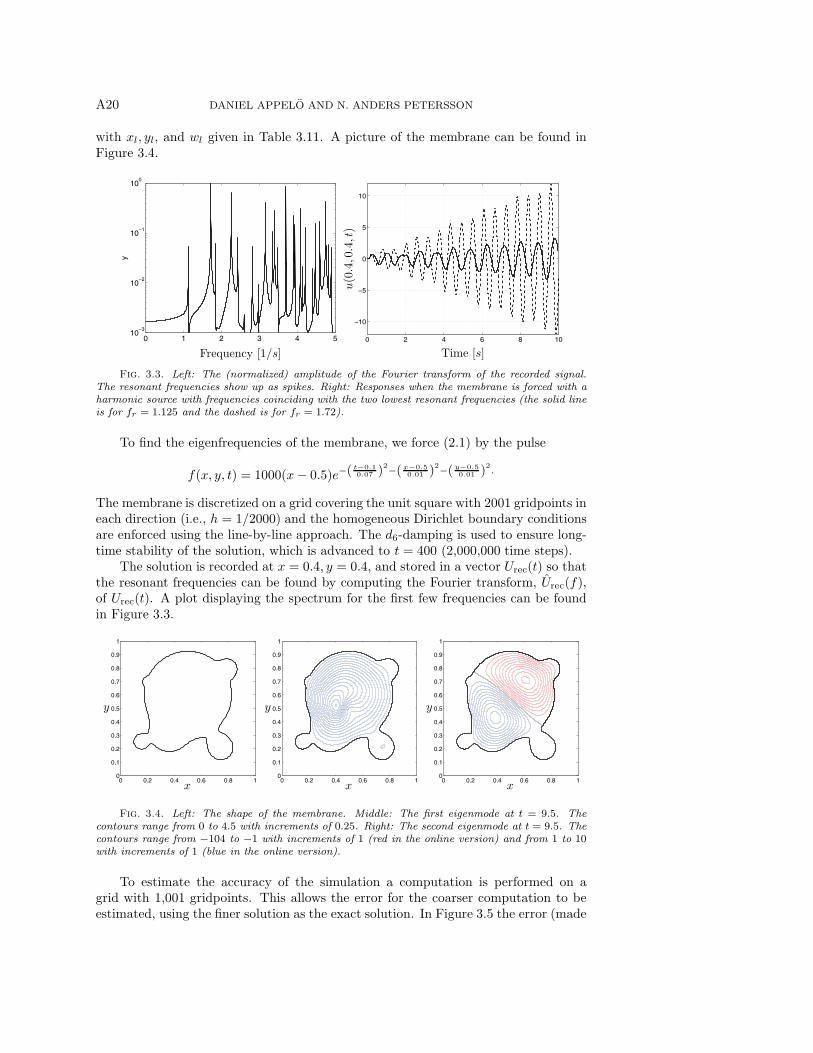
with xl, yl, and wl given in Table 3.11. A picture of the membrane can be found inFigure 3.4.

0 1 2 3 4 510

−3

10−2

10−1

100

y

Frequency [1/s]

0 2 4 6 8 10

−10

−5

0

5

10

Time [s]u(0.4,0.4,t)

Fig. 3.3. Left: The (normalized) amplitude of the Fourier transform of the recorded signal.The resonant frequencies show up as spikes. Right: Responses when the membrane is forced with aharmonic source with frequencies coinciding with the two lowest resonant frequencies (the solid lineis for fr = 1.125 and the dashed is for fr = 1.72).

To find the eigenfrequencies of the membrane, we force (2.1) by the pulse

f(x, y, t) = 1000(x− 0.5)e−(t−0.10.07 )

2−(x−0.50.01 )

2−( y−0.50.01 )

2.

The membrane is discretized on a grid covering the unit square with 2001 gridpoints ineach direction (i.e., h = 1/2000) and the homogeneous Dirichlet boundary conditionsare enforced using the line-by-line approach. The d6-damping is used to ensure long-time stability of the solution, which is advanced to t = 400 (2,000,000 time steps).

The solution is recorded at x = 0.4, y = 0.4, and stored in a vector Urec(t) so thatthe resonant frequencies can be found by computing the Fourier transform, Urec(f),of Urec(t). A plot displaying the spectrum for the first few frequencies can be foundin Figure 3.3.

0 0.2 0.4 0.6 0.8 10

0.1

0.2

0.3

0.4

0.5

0.6

0.7

0.8

0.9

1

x

y

0 0.2 0.4 0.6 0.8 10

0.1

0.2

0.3

0.4

0.5

0.6

0.7

0.8

0.9

1

x

y

0 0.2 0.4 0.6 0.8 10

0.1

0.2

0.3

0.4

0.5

0.6

0.7

0.8

0.9

1

x

y

Fig. 3.4. Left: The shape of the membrane. Middle: The first eigenmode at t = 9.5. Thecontours range from 0 to 4.5 with increments of 0.25. Right: The second eigenmode at t = 9.5. Thecontours range from −104 to −1 with increments of 1 (red in the online version) and from 1 to 10with increments of 1 (blue in the online version).

To estimate the accuracy of the simulation a computation is performed on agrid with 1,001 gridpoints. This allows the error for the coarser computation to beestimated, using the finer solution as the exact solution. In Figure 3.5 the error (made


relative by the maximum amplitude of the fine solution) in the time history, is plotted.As can be seen, the maximum relative error in the coarse solution is estimated to beabout 1%. As the method is fourth-order accurate it is expected that the error inthe fine grid solution is about sixteen times smaller. Figure 3.5 also displays theFourier transform, Urec(f) of the two computations. Only the small peak with anrelative amplitude of 10−2 at 2.6 Hz is visibly different, this is consistent wit theabove accuracy estimate.

0 1 2 3 4 510

−3

10−2

10−1

100

|Urec.|

Frequency [1/s]0 50 100 150 200 250 300 350 400

−0.01

−0.005

0

0.005

0.01

Time [s]

Relativeerror

Fig. 3.5. Left: The (normalized) amplitude of the Fourier transform of the recorded signal forsimulations using h = 1/1000 (dashed red) and h = 1/2000 (solid black). Only the small peak at 2.6Hz is visibly different. Right: Relative error in the time history, Urec(t), for the coarse simulation.

Once the frequencies are found, the eigenmodes can be approximated by forcingthe problem with a harmonic source at the resonant frequency. Here we have forcedit with

f(x, y, t) = 200

(−2

(x− 0.45)

0.052

)sin(2πfrt) e

− (x−0.45)2+(y−0.4)2

0.052 ,

for fr = 1.125 and fr = 1.72. In Figure 3.3 the response at x = 0.4, y = 0.4 is plottedas a function of time. As expected, the amplitude grows linearly for a resonantfrequency. Figure 3.4 plots the two first eigenmodes.

We note that this experiment is only meant to serve as an illustration of howresonant frequencies can be extracted using time-dependent simulations and that thereare modern methods [25, 31] that significantly accelerates the above procedure.

3.6. A radiating unidentified object in free space. In the final experimentwe study the radiation from an unidentified object in free-space. The purpose of thisexperiment is to demonstrate the use of nonreflecting boundary conditions togetherwith the proposed method on a problem where the solution is propagated over manywavelengths.

The geometry of the unidentified object is defined as the zero contour of

ϕ(x, y) = 0.5− 1.0e−(

x2

0.32+ y2

0.042

)− 1.2e

−(

x2

0.052+ (y−0.06)2

0.032

);

see Figure 3.6. The object is placed in a rectangular domain (x, y) ∈ [−1, 1]2 dis-cretized on a grid with spacing h = 2/N and a sequence of grids N = 400, 800, 1600.On the boundary of the object, we prescribe Dirichlet data in form of a smoothlystarted plane wave

u(x, y, t) = (1− e−5t5) cos(ω(x− t)), (x, y) ∈ Γ, t ≥ 0, ω = 150.


1

2

3

4

30

210

60

240

90

270

120

300

150

330

180 0

Fig. 3.6. Left: Snapshot of u(x, y, 3). The pictured domain is (x, y) ∈ [−0.75, 0.75]2. Right:The quantity Q is plotted.

The outer, free-space, boundary condition is modeled by truncating the domainusing a perfectly matched layer (derived in Appendix A)

(3.6) utt =∂

∂x

(ux + σ(x)φ(1)

)+

∂

∂y

(uy + σ(y)φ(2)

)+ σ(x)φ(3) + σ(y)φ(4),

where the auxiliary variables satisfy the equations

φ(1)t + (α+ σ(x))φ(1) = −ux,

φ(2)t + (α+ σ(y))φ(2) = −uy,

φ(3)t + (α+ σ(x))φ(3) = −uxx − ∂

∂x

(σ(x)φ(1)

),

φ(4)t + (α+ σ(y))φ(8) = −uyy − ∂

∂y

(σ(y)φ(2)

).

(3.7)

The damping profiles σ(z)(z), z = x, y, are taken as

σ(z)(z) =σmax

2

(2 + tanh

(z − zpml

δpml

)− tanh

(z + zpml

δpml

)),

with σmax = 15, zpml = 0.75, δpml = 0.01. The complex frequency shift is chosen asα = 0.05.

Now, as the modified equation approach is used to obtain a high-order-accuratetime discretization we must compute

utttt =∂2

∂x2(utt) +

∂2

∂y2(utt)

+∂2

∂t2

(∂

∂x(σ(x)φ(1)) +

∂

∂y(σ(y)φ(2)) + σ(x)φ(3) + σ(y)φ(4)

)︸︷︷︸

F

.(3.8)

We note that once (3.6) is computed, the first two terms in (3.8) can be approximatedusing the compact scheme. The third term must be approximated to second-orderaccuracy. In this case it is done by first advancing the auxiliary variables using the


0 0.5 1 1.5 2 2.5 3

10−4

10−3

10−2

10−1

45◦

Relativeerror

Time

0 0.5 1 1.5 2 2.5 3

10−4

10−3

10−2

10−1

135◦

Relativeerror

Time

0 0.5 1 1.5 2 2.5 3

10−4

10−3

10−2

10−1

225◦

Relativeerror

Time

0 0.5 1 1.5 2 2.5 3

10−4

10−3

10−2

10−1

315◦Relativeerror

Time

Fig. 3.7. Relative errors for time traces of the solution at four angles. The black, red, and bluelines are for errors using N = 400, 800, 1600 grid points in each direction. The reference solution isobtained by Richardson extrapolation of the two finest grids.

classic fourth-order-accurate Adams method [15] to get φ(x, y, tn+1) so Fn+1 canbe computed. In our implementation a compact fourth-order-accurate method isused to approximate the first derivatives in F . Once Fn+1 is found, a second-orderapproximation is given by

∂2

∂t2Fn ≈ Fn+1 − 2Fn + Fn−1

k2.

With the PML in place, the solution is advanced to t = 3, at which time moststart-up transients have exited the computational domain and the solution has reacheda time-harmonic state. The line-by-line approach is used to enforce the boundaryconditions and the d6-damping is used to stabilize the scheme.

In order to compute the radiation pattern, the solution is recorded at (x, y) =(0.5 cos θ, 0, 5 sin θ), θ = 0, dθ, . . . , 2π, dθ = 2π/360 at each time step. In the rightimage of Figure 3.6, the quantity

Q = log10

(I(θ)

minθ I(θ)

),


is plotted. I(θ) is an intensity defined as the time integral of the square of the solutionduring one period, T = 2π/ω,

I(θ) =

∫ 2+ 2πω

2

|u(0.5 cos θ, 0.5 sin θ, τ)|2 dτ.

The results of the simulation can be found in Figure 3.6. The left image showsa snapshot of the solution at t = 3. The wavelength, λ, is about 0.04, so the totaldomain is ∼ 50λ wide and the unidentified object is ∼ 12λ wide. Note that only(x, y) ∈ [−0.8, 0.8]2 is displayed in the figure. The snapshot is for the finest grid andhas about 32 points per wavelength. To the right we had exploited the Q, definedabove, for the finest grid (in black) and for a Richardson extrapolation of the twofinest grids (in red). The difference is very small.

To estimate the accuracy of the solution we compare time series of the solutionrecorded at angles 45, 135, 225, and 315 degrees. The solutions on the three grids arecompared to the Richardson extrapolated value based on the two finest grids. Therelative error obtained from this comparison, that can be found in Figure 3.7, showsthat the grid with 16 points per wavelength has errors well below 1% and should begood for engineering accuracies. In summary this example demonstrates our methodscapability to simulate wave propagation problems with many wavelengths as well ascomplex geometry at engineering accuracy.

4. Conclusions. In summary, we have derived and demonstrated the applica-bility of a fourth-order-accurate embedded boundary method for the wave equation.In our view, the strength of the method is its high-order of accuracy along with itsrelative simplicity. The fact that the method consist of separate building blocks thatcan easily be adjusted if other PDE or applications are considered is another strength.

There are many possible extensions of the method that are worth considering.These include

1. Generalize the method to Maxwell’s equations formulated as a system ofsecond-order equations.

2. Adopting the approach to compressible flow problems. This has been suc-cessfully done in [27, 13] for the earlier second-order-accurate methods.

3. Raising the order of accuracy further. Raising the order of the compactmethod to six is possible by increasing the bandwidth of the linear systemfrom three to five. Extending the temporal discretization and raising the orderof the boundary stencils should also be straightforward but might require thatnew damping terms are considered.

4. Experimentation with other spatial and temporal discretizations, in particularsummation-by-parts finite difference discretizations [12].

5. Generalization of the proposed method to three dimensions. For the dimension-by-dimension approach the extension to three dimensions (3D) is straightfor-ward. If the boundary conditions are enforced by interpolation in the normaldirection extension to 3D conceptually straightforward but the implementa-tion is more involved. We note that three-dimensional versions of the relatedsecond-order schemes [9, 10, 11] have been implemented (but not yet pub-lished).

6. Inhomogeneous materials. For smoothly varying materials the current schemecould be extended by evaluating terms like (c(x)ux)x either by applying acompact discretization of the first derivative twice or by expanding (c(x)ux)xto c(x)uxx + cx(x)ux. Note that the right-hand side of (2.9) will be more


expensive to evaluate for a smoothly varying material. For sharp materialinterfaces it might be possible to extend the approach suggested in [8].

Finally, we note that this paper has mainly focused on the description of themethod along with several numerical experiments and largely avoided detailed analysisof the discretization. The rationale for this emphasis is twofold. First, detailedanalysis of the EB-methods of the type considered here has already been presentedfor the related second-order-accurate methods in [9, 10, 11]. Analysis of the presentmethod would largely follow along the lines of [9, 10, 11]. It would be algebraicallymore involved but probably lead to similar conclusions: there are weak instabilitiesthat can be suppressed by suitably chosen artificial dissipation. Second, an aim of thispaper was to promote the use of embedded boundary methods and we thus focused ondescribing the algorithms in sufficient detail to make them replicable by the interestedreader.

Appendix A. PML with modified equation time-stepping. To be able totreat unbounded domains we enclose the computational domain within a perfectlymatched layer. Following [3] we perform the usual s (s is the Laplace transformvariable dual of t) dependent coordinate stretching and get

(A.1) ρs2u =

(1− σ(x)

s+ α+ σ(x)

)∂

∂x

((1− σ(x)

s+ α+ σ(x)

)∂

∂xu

)

+

(1− σ(y)

s+ α+ σ(y)

)∂

∂y

((1− σ(y)

s+ α+ σ(y)

)∂

∂yu

).

To localize we introduce the auxiliary variables

φ(1) = − 1

s+ α+ σ(x)

∂

∂xu, φ(2) = − 1

s+ α+ σ(y)

∂

∂yu,

φ(3) = − 1

s+ α+ σ(x)

∂

∂x

((1− σ(x)

s+ α+ σ(x)

)∂

∂xu

),

φ(4) = − 1

s+ α+ σ(y)

∂

∂y

((1− σ(y)(y)

s+ α+ σ(y)

)∂

∂yu

).

This leads to the perfectly matched layer model (3.6) with auxiliary equations (3.7).

Appendix B. Artificial dissipation. Acting on a one-dimensional grid func-tion qi, i = 1, . . . , s, the fourth-order operator wi = D4qi is

w1 = q1 − 2q2 + q3,

w2 = −2q1 + 5q2 − 4q3 + q4,

wi = 6qi − 4(qi+1 + qi−1 + qi+2 + qi−2), i = 3, . . . , s− 2.

The sixth-order operator wi = D6qi is

w1 = −3q1 + 9q2 − 9q3 + 3q4,

w2 = 9q1 − 28q2 + 30q3 − 12q4 + q5,

w3 = −9q1 + 30q2 − 37q3 + 21q4 − 6q5 + q6,

w4 = 3q1 − 12q2 + 21q3 − 22q4 + 15q5 − 6q6 + q7,

wi = −20qi + 15(qi−1 + qi+1)− 6(qi−2 + qi+2) + (qi−3 + qi+3), i = 5, . . . , s− 4.


The eight-order operator wi = D8qi is

w1 = 3q1 − 12q2 + 18q3 − 12q4 + 3q5,

w2 = −12q1 + 49q2 − 76q3 + 54q4 − 16q5 + q6,

w3 = 18q1 − 76q2 + 125q3 − 100q4 + 40q5 − 8q6 + q7,

w4 = −12q1 + 54q2 − 100q3 + 101q4 − 64q5 + 28q6 − 8q7 + q8,

w5 = 3q1 − 16q2 + 40q3 − 64q4 + 72q5 − 56q6 + 28q7 − 8q8 + q9,

wi = 70qi − 56(ui−1 + ui+1) + 28(ui−2 + ui+2)− 8(ui−3 + ui+3) + 1(ui−4 + ui+4),

i = 6, . . . , s− 5.

REFERENCES

[1] B. Alpert, L. Greengard, and T. Hagstrom, An integral evolution formula for the waveequation, J. Comput. Phys., 162 (2000), pp. 536–543.

[2] L. Anne, P. Joly, and H. Q. Tran, Construction and analysis of higher order finite differenceschemes for the 1d wave equation, Comput. Geosci., 4 (2000), pp. 207–249.

[3] D. Appelo and G. Kreiss, Application of a perfectly matched layer to the nonlinear waveequation, Wave Motion, 44 (2007), pp. 531–548.

[4] O. Bruno and M. Lyon, High-order unconditionally-stable FC-AD solvers for general smoothdomains. I. Basic elements, J. Comput. Phys., 229 (2010), pp. 2009–2033.

[5] L. Collatz, The Numerical Treatment of Differential Equations, 3rd ed., Springer-Verlag,Berlin, 1960.

[6] M. A. Dablain, The application of high-order differencing to the scalar wave equation, Geo-physics, 51 (1986), pp. 54–66.

[7] H.-O. Kreiss and J. Oliger, Comparison of accurate methods for the integration of hyperbolicequations, Tellus, 24 (1972), pp. 199–215.

[8] H.-O. Kreiss and N. A. Petersson, An embedded boundary method for the wave equationwith discontinuous coefficients, SIAM J. Sci. Comput., 28 (2006), pp. 2054–2074.

[9] H.-O. Kreiss and N. A. Petersson, A second order accurate embedded boundary method forthe wave equation with Dirichlet data, SIAM J. Sci. Comput., 27 (2006), pp. 1141–1167.

[10] H.-O. Kreiss, N. A. Petersson, and J. Ystrom, Difference approximations for the secondorder wave equation, SIAM J. Numer. Anal., 40 (2002), pp. 1940–1967.

[11] H.-O. Kreiss, N. A. Petersson, and J. Ystrom, Difference approximations of the Neumannproblem for the second order wave equation, SIAM J. Numer. Anal., 42 (2004), pp. 1292–1323.

[12] H.-O. Kreiss and G. Scherer, Finite Element and Finite Difference Methods for Hyper-bolic Partial Differential Equations, in Mathematical Aspects of Finite Element in PartialDifferential Equations, Academic Press, New York, 1974.

[13] M. Kupiainen and B. Sjogreen, A Cartesian embedded boundary method for the compressibleNavier-Stokes equations, J. Sci. Comput., 41 (2009), pp. 94–117.

[14] S. K. Lele, Compact finite difference schemes with spectral-like resolution, J. Comput. Phys.,103 (1992), pp. 16–42.

[15] R. J. LeVeque, Finite Difference Methods for Ordinary and Partial Differential Equations:Steady-State and Time-Dependent Problems, SIAM, Philadelphia, 2007.

[16] J.-R. Li and L. Greengard, High order marching schemes for the wave equation in complexgeometry, J. Comput. Phys., 198 (2004), pp. 295–309.

[17] B. Lombard and J. Piraux, Numerical treatment of two-dimensional interfaces for acousticand elastic waves, J. Comput. Phys., 195 (2004), pp. 90–116.

[18] B. Lombard, J. Piraux, C. Gelis, and J. Virieux, Free and smooth boundaries in 2-d finite-difference schemes for transient elastic waves, Geophys. J. Internat., 172 (2008), pp. 252–261.

[19] M. Lyon, High-Order Unconditionally-Stable FC-AD PDE Solvers for General Domains, Ph.D.thesis, California Institute of Technology, Pasadena, CA, 2009.

[20] M. Lyon and O. Bruno, High-order unconditionally stable FC-AD solvers for general smoothdomains. II. Elliptic, parabolic and hyperbolic PDEs; theoretical considerations, J. Com-put. Phys., 229 (2010), pp. 3358–3381.

[21] K. Mattsson, M. Svard, and J. Nordstrom, Stable and accurate artificial dissipation, J. Sci.Comput., 21 (2004), pp. 57–79.


[22] P. Olsson, The numerical behavior of high-order finite difference methods, J. Sci. Comput.,9 (1994), pp. 445–466.

[23] R. B. Pember, J. B. Bell, P. Colella, W. Y. Crutchfield, and M. L. Welcome, An adap-tive Cartesian grid method for unsteady compressible flow in irregular regions, J. Comput.Phys., 120 (1995), pp. 278–304.

[24] C. S. Peskin, Flow patterns around heart valves: A numerical method, J. Comput. Phys., 10(1972), pp. 252–271.

[25] T. Rylander, T. McKelvey, and M. Viberg, Estimation of resonant frequencies and qualityfactors from time domain computations, J. Comput. Phys., 192 (2003), pp. 523–545.

[26] G. R. Shubin and J. B. Bell, A modified equation approach to constructing fourth-ordermethods for acoustic wave propagation, SIAM J. Sci. Statist. Comput., 8 (1987), pp. 135–151.

[27] B. Sjogreen and N. A. Petersson, A Cartesian embedded boundary method for hyperbolicconservation laws, Commun. Comput. Phys., 2 (2007), pp. 1199–1219.

[28] J. Visher, S. Wandzura, and A. White, Stable, high-order discretization for evolution of thewave equation in 1 + 1 dimensions, J. Comput. Phys., 194 (2004), pp. 395–408.

[29] S. Wandzura, Stable, high-order discretization for evolution of the wave equation in 2 + 1dimensions, J. Comput. Phys., 199 (2004), pp. 763–775.

[30] R. Weller and H. Shortely, Calculation of stresses within the boundary of photoelasticmodels, J. Appl. Mech., 6 (1939), pp. A71–A78.

[31] G. R. Werner and J. R. Cary, Extracting degenerate modes and frequencies from time-domain simulations with filter-diagonalization, J. Comput. Phys., 227 (2008), pp. 5200–5214.

Documents

A FOURTH-ORDER ACCURATE EMBEDDED BOUNDARYappelo/preprints/077223.pdf · A fourth-order accurate embedded boundary method for the scalar wave equation ... problem for both Dirichlet