NASA Technical Memorandum 87104 JNASA-TM-8710419860003827

A FORTRAN Computer Code for Calculating Flows in Multiple-Blade-Element Cascades

Eric R. McFarland Lewis Research Center Cleveland, Ohio

November 1985

Nl\51\

,.- #-

: ..• ::; .! ~ ~~; .~';.~:: .• : .:./

.... -' ~ : " "- ',: . ~.'! .' , . ..: 1 ..'

.' IU~HDU'IHHHIDUIHIIII~IIR ' ~

https://ntrs.nasa.gov/search.jsp?R=19860003827 2020-02-10T21:06:09+00:00Z

A FORTRAN COMPUTER CODE FOR CALCULATING FLOWS

IN MULTIPLE-BLADE-ELEMENT CASCADES

by

Er1c R. McFarland National Aeronaut1cs and Space Adm1n1strat1on

Lew1s Research Center Cleveland, Oh10 44135

SUMMARY

A solut10n techn1que has been developed for solv1ng the mult1ple-blade­element, surface-of-revolut10n, blade-to-blade flow problem 1n turbomach1nery. The calculat10n solves approx1mate flow equat10ns wh1ch 1nclude the effects of compress1b1l1ty, radius change, blade-row rotat10n, and var1able stream sheet th1ckness. An 1ntegral equat10n solution (1.e., panel method) 1s used to solve the equat10ns. A descript10n of the computer code and computer code 1nput is g1ven 1n th1s report.

INTRODUCTION

A computer code has been wr1tten to analyze flow on turbomach1nery blade­to-blade surfaces. The code has the capab1l1ty of analyz1ng blade rows which are made up of several d1fferent blade shapes and/or spac1ngs. Th1s capab111ty makes the code useful for calculating flows in centrifugal mach1nery w1th sp11tter blades or 1n mis-tuned blade rows, where the blade spacing varies. The number of varying blade shapes that can be used 1n a blade-row des1gn 1s not limited by the code. However, the amount of computer storage available does impose a practical limit on any problem. The code being described here 1s dimensioned to handle from one to four bodies in cascade. After redimensioning, this same code has been used to calculate a flow problem w1th as many as 15 bodies.

The basic method used to solve the flow field was described in reference 1. However, the method of reference 1 was extended 1n the code reported here to 1nclude multiple-body cascades. Briefly, the solut1on method solves approx1-mate governing equations for the b1ade-to-blade, steady-state flow problem in turbomachinery. The effects of compressib111ty, radius change, blade-row rota­t10n. and variable stream sheet thickness are 1neluded. The work1ng flu1d 1s assumed to be 1nv1scid, irrotat1onal, and a perfect gas. Comparisons w1th other solution techniques and experimental data is g1ven in reference 1. Overall, the solution produces good results for subson1c flow. but the accuracy decrea­ses for high subson1c and supersonic flows.

CODE DESCRIPTION

General

The multip1e-body-panel code is written primar11y 1n FORTRAN IV, and uses double prec1s1on ar1thmet1c. storage for the four-body version of the code,

which accompanies this report, is approximately 650 000 words when run in double precision. Typical run times for the code on the IBM 370/3033 computer at NASA Lewis is 25 CPU sec. A slightly different version of the code which runs on the CRAY lS computer at NASA Lewis requires less than 5 CPU sec/run.

The computer code accompanying this report is essentially the version of the code that runs on the CRAY computer. However, coding that is CRAY computer dependent and allows vector1zat1on of the calculation has been replaced with scalar coding which is machine independent. Also, calls to the Society of Industrial and Applied Mathematics (SIAM) matrix solvers contained in their LINPACK software package have been replaced by calls to an in-house generated solver which is included with the code. The result of these code changes is a code which is slower running than the version of the code used at NASA Lewis, but is more machine and system independent. If the user has access to SIAM's LINPACK software, instructions on how to 1mpl1ment it into the code are g1ven 1n the comment statements of subrout1ne PLMSOL.

Some machine dependency was left in the code. The code is set up w1th the cod1ng for variable storage arrays and dimensions separated from the main body of the code. On both the IBM and CRAY computer systems at NASA Lewis, this cod1ng is inserted into the main code by the comp11er. This comp111ng option allows the user to adjust the storage requirements of the code and to increase (or decrease) the number of bodies which can be cons1dered. The option 1s ava11able on many computing systems, and so the code's structure was left .1n this form. If the user's system does not have this capability, he can phys1-cally dimens10n the arrays and insert the coding 1nto the program before com­p1l1ng.

Code Structure

The code on the tape as given to COSMIC consists of several short p1eces of coding followed by the main code and its accompanying subroutines. The short pieces of coding contain the var1able array and dimensioning 1nformat10n. These segments are inserted into the main coding during compilation. This coding appears first on the tape. Each segment is preceded by a line that reads "*CDK" followed by the name of the segment. F1ve of these segments are used in the code. Each segment is inserted into the program wherever the cod­ing "*CALL" followed by the name of the segment appears. The main program and subroutines are given next on the tape. A line reading "*DK" followed by the name of the routine precedes each subroutine and the main program. The multi­ple body panel code consists of the main program plus 24 subroutines.

The multiple body panel code is written in a modular style. No calcula­tions or input/output takes place in the main program. The main program only serves as a calling routine. Each subroutine then performs a particular func­tion in the overall solution. The various parts of the code are listed below along with a brief description of the coding's function. Items are 11sted in the order that they should appear on the tape.

2

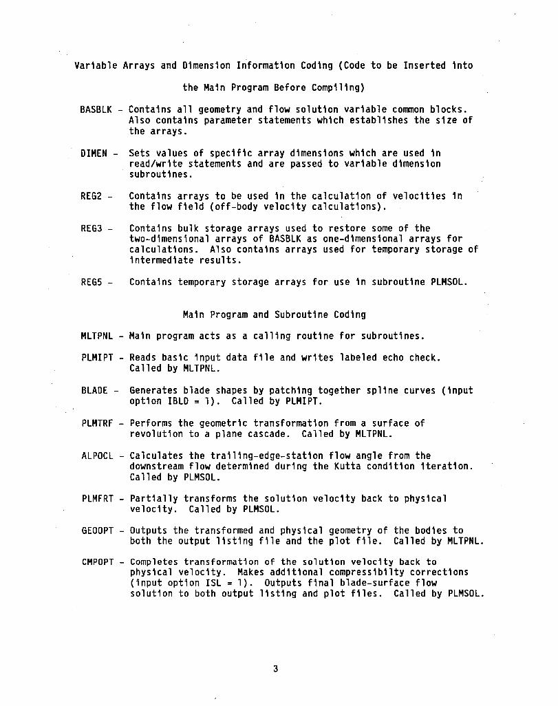
Variable Arrays and Dimension Information Cod\ng (Code to be Inserted into

the Main Program Before Compiling)

BASBLK - Contains all geometry and flow solution variable common blocks. Also contains parameter statements which establishes the size of the arrays.

DIMEN - Sets values of specific array dimensions which are used in read/write statements and are passed to variable dimension subroutines.

REG2 - Contains arrays to be used in the calculation of velocities in the flow field (off-body velocity calculations).

REG3 - Contains bulk storage arrays used to restore some of the two-dimensional arrays of BASBLK as one-dimensional arrays for calculations. Also contains arrays used for temporary storage of intermediate results.

REG5 - Contains temporary storage arrays for use in subroutine PLMSOL.

Main Program and Subroutine Coding

MLTPNL - Main program acts as a calling routine for subroutines.

PLMIPT - Reads basic input data file and writes labeled echo check. Called by MLTPNL.

BLADE - Generates blade shapes by patching together spline curves (input option IBLD = 1). Called by PLMIPT.

PLMTRF - Performs the geometric transformation from a surface of revolution to a plane cascade. Called by MLTPNL.

ALPOCL - Calculates the tra11ing-edge-stat1on flow angle from the downstream flow determined during the Kutta condition iteration. Called by PLMSOL.

PLMFRT - Partially transforms the solution velocity back to physical velocity. Called by PLMSOL.

GEOOPT - Outputs the transformed and physical geometry of the bodies to both the output listing file and the plot file. Called by MLTPNL.

CMPOPT - Completes transformation of the solution velocity back to physical velocity. Makes additional compressibi1ty corrections (input option ISL = 1). Outputs final blade-surface flow solution to both output listing and plot files. Called by PLMSOL.

3

RBINT - Calculates the one-d1mens10nal, compressible flow used in approxi­mate governing equat1oris. Also performs integrations to get con­tr1but16nsof the com~ress1b1l1ty, blade-row rotation, and stream sheet th1ckness variation to the flow solution. Called by PLMSOL.

PLMSOL - Sets up the system of equations to be solved. Acts as a secondary calling routine which brings together all the subrout1nes and information used to solve the matr1x of equations for the flow. Called by MLTPNL.

PLMGEO - Calculates geometr1c parameters and var1ables used 1n the solution. Called by MLTPNL.

KCGEOM - Calculates the points downstream of the trailing edges and the flow angles to be used in the Kutta cond1t10n (input option ICSCD = 0, 2, or 3). Called by PLMGEO.

VORTEX - Calculates influence of a linear vortex singularity distribution. Called by ABCOEF and OFFBOD.

ABCOEF - Acts as a secondary calling routine to call the subrout1nes which calculate the influence coefficients of the integral-equation solution. Called by MLTPNL.

JUMP - Calculates the influence coefficients for a discontinuous change in a vortex s1ngular1ty distribution wh1ch is due to discontin­uous changes in the slope of the surface of a body. Called by ABCOEF and OFFBOD.

SOURCE - Calculates influence coefficients of a linear-source singular1ty d1str1but10n. Called by ABCOEF and OFFBOD.

VELCAL - Calculates the velocity influence coefficient due to source and vortex d1str1but10ns for 1solated bod1es. Called by ABCOEF and OFFBOD.

CASCAD - Calculates the velocity influence coefficients due to source and vortex distributions for a cascade of bodies. Called by ABCOEF and OFFBOD.

BNDCND - Calculates the far-stream boundary cond1t1ons from the 1nput flow conditions at the blade lead1ng- and tra1l1ng-edge stat19ns. Called by PLMSOL.

POTOPT - Outputs the transformed veloc1t1es and singularity strength d1str1but1on. Used primarily for solution debugging. Called by PLMSOL.

SPLINT - Calculates a sp11ne curve f1t and 1nterpolat1on from a given array of data points. Assumes the second der1vat1ve of the curve goes to zero at the end points. Also has an entry p01nt SPLENT for multiple interpolations along the same curve. Called by BLADE, PLMGEO, PLMTRF, PLMSOL, BNDCND, RBINT, and OFFBOD.

4

SPINSL - Calculates a spline curve fit and interpolation from a given array of data points. Uses the given slope at the curve ends to calcu­late the sp11ne curve f1t. Called by BLADE.

OFFBOD - Reads coordinates of points that the user has specified. Calcu­lates the flow velocity and direction at those points. Writes out body velocity information to both the output listing and plot f1les. Called by CHPOPT.

CHLSKY - Solves a set of linear equat10ns by upper and lower triangular matrix decomposition. Has an entry point called CHGCNT for repeat solutions of the same system of equations with a different right hand side. Called by PLMSOL.

CFCALC - Calculates the tangent1a1 and normal force coefficients for each body. Also calculates 11ft. drag. and moment coeff1c1ents. Outputs results to the output l1st1ng file. Called by CMPOPT.

Input, Output, and Storage F1les

The mult1ple-body-panel code 1s reasonably straightforward to set up and run. The 1nput data f11e 1s column formated. All numer1cal data 1s e1ther 8F10.0 for float1ng point or 1615 for fixed point data. Floating and f1xed p01nt data are not mixed on any input line. Deta1ls of the input data f11e are g1ven 1n a separate section of th1s report. Input 1s read in from unit OS, and pr1nted output 1s sent to unit 06. In addition, an unformated binary output data set can be sent to unit 60. This binary data set contains geo­metric and flow solut10n 1nformat1on. It is intended for use in any graph1cs code that the user may develop. A descr1pt10n of the 1nformat10n in th1s "graphics" file w1ll be g1ven later. In order to reduce the 1n-core storage needed to run the code, extens1ve use is made of mass storage dev1ces. Th1s requ1res that units 10 to 20 be ass1gned when runn1ng the code. These un1ts are used str1ctly as scratch storage and should be released upon complet10n of the calculat10n.

The use of mass storage (un1ts 10 to 20) 1s a trade-off of run time for computer storage. If the user wants a faster running code and has a large­memory computer system available, he may want to eliminate the out-of-core reads and writes. The exper1ence of the author 1s that this 1ncreases the required 1n-core storage by about a factor of five for the four-body problem (from 0.65 to 4 M words).

The convers10n of the code to run using only 1n-core storage 1s not a s1mple task. F1rst, the user must locate all the 1n1t1al wr1tes to un1ts 10 to 20. These are located 1n subrout1nes ABCOEF, OFFBOD, and PLHSOL. Second, the user must def1ne two-d1mens1onal arrays to store the values that had prev-10usly been written out and read 1n from out-of-core storage. Th1rd, the user must subst1tute the new var1ables 1nto the solut1on equat10ns w1th the proper 1nd1ces. Lastly, the user must remove all read and wr1te statements to un1ts 10 to 20.

5

Code-Generated D1agnost1c Messages

Several messages can appear 1n the pr1nted output from the mult1ple-body code. The name of the subrout1ne generat1ng the message 1s appended to the end of the message. The messages are 11sted together along w1th a d1scuss10n of what occurs 1n the calculat10n when the message appears.

1. THE AVERAGE PANEL IS SMALLER THAN THE ADJACENT L. E. OR T. E. PANELS - NS OR NE IS LESS THAN ZERO. THE PERCENTAGE OF POINTS IN THE LEADING EDGE HAS BEEN INCREASED. PLE IS NOW - BLADE

The blade shape generator was set up assum1ng that the elements used to descrlbe the leadlng and tra111ng edges would be smaller than the elements used to descr1be the blade surface. If the user spec1fles 1nput parameters that vl01ate th1s cond1t10n, the code wl11 lncrease the number of elements used to descrlbe the lead1ng edge unt11 the lead1ng-edge elements are smaller than the surface elements. Everytlme the message ls prlnted, 5 percent of the total number of elements to be used ln descrlblng the blade are added to the leadlng-edge elements. Increaslng the number of leadlng-edge polnts does not always allow the solutlon to contlnue. If the tral11ng-edge radlus ls large compared to the leadlng edge and has panels that are larger than the average blade surface panel, then the blade shape generator wl11 fall to glve a dlstrl­butlon of panel elements that wl11 allow the calculatlon to proceed. In these cases, the user wl11 have to provlde the code wlth a descrete polnt descr1ptlon of the lnput body.

2. THE DOWNSTREAM FLOW CALCULATION IN SUBROUTINE ALPOCL IS IN ERROR - PLMSOL

Th1s error message can appear ln solutlons uslng the Kutta cond1tlon optlon. It lndlcates that the downstream flow angle, calculated uslng the blade-row clrculatlon, exceeds the maxlmum posslble turnlng angle for the flow. The downstream angle ls set to the maxlmum value so that the calculatlon may proceed.

3. KUTTA CONDITION HAS FAILED TO FIND A SOLUTION IN 100 ITERATIONS. ERROR IN THE INLET FLOW ANGLE IS RADIANS - PLMSOL

The Kutta condltlon lteratlon (ICSCD = 0, 2, or 3 In the lnput) has fal1ed to converge to the glven lnput flow. The calculatlon wl11 contlnue using the flow fleld at the 100th lteratlon. If the error ls large, the calculated results wlll be lnvalld.

4. ITERATION FOR (UPSTREAM/OUTLET/DOWNSTREAM) FLOW CONDITIONS HAS FAILED TO CONVERGE. ERROR IS - BNDCND

Us1ng the glven lnlet flow condltlons, the solutlon calculates a mass flow for the blade passage. Flow condlt10ns at the upstream, downstream, and outlet blade-row statlons are then calculated. If the lteratlon procedure lnvolved 1n solvlng the equat10ns does not converge In 100 lterat10ns, the above message· ls prlnted with the approprlate station noted, and the calculatlon is allowed to contlnue.

6

5. SPECIFIED INLET FLOW EXCEEDS CHOKING MASS FLOW - BNDCND

If the g1ven 1nlet flowcond1t1ons def1ne a flow that exceeds the chok1ng mass flow, the above message 1s pr1nted. The calculat10n cont1nues but the solut1on 1s 1nva11d.

6. SPECIFIED OUTLET FLOW EXCEEDS CHOKING FLOW - BNDCND

7. GIVEN OUTLET FLOW ANGLE EXCEEDS MAXIMUM ALLOWABLE - IT HAS BEEN LOWERED TO - BNDCND

The above two messages are pr1nted when the outlet flow angle produces a flow that 1s greater then the max1mum flow poss1ble. The flow angle 1s adjus­ted to produce the max1mum flow at the ex1t, and the calculat10n cont1nues. The messages can be d1sregarded for Kutta cond1t1on calculat1ons, s1nce the f1nal outlet flow cond1t1ons are determ1ned later 1n the calculat1on.

8. MAXIMUM OR NEGATIVE VELOCITY ENCOUNTERED AT (UPSTREAM/DOWNSTREAM) BOUNDARY - (UPSTREAM/DOWNSTREAM) RADIUS TOO SMALL? - BNDCND

Th1s message 1nd1cates that the cr1t1cal veloc1ty rat10 has exceeded·the max1mum value at e1ther of the far-stream stat10ns as noted. Th1s can occur 1n rad1al mach1nery 1f the far-stream boundary cond1t1on 1s taken at too small a rad1us. For rotors, the error can also occur1f the rad1us 1s too large. The solut1on cont1nues, but 1t 1s 1nva11d. The user can avo1d the error by mov1ng the boundary stat10n (MRSP(l) or MRSP(NMN) 1n the 1nput) 1n closer to the blade row.

9. AVERAGE MASS FLOW CALCULATION EXCEEDS CHOKING FLOW AT M =. CALCULATED AVERAGE MASS FLOW IS TIMES THE CHOKING MASS FLOW. THE FLOW TURNING ANGLE HAS BEEN REDUCED TO ALLOW THE CHOKING MASS FLOW TO PASS - RBINT

Th1s message can occur for calculat10ns us1ng the blade-passage geometry and one-d1mens1onal cont1nu1ty to calculate the mean flow est1mates. The cal­culat10n 1s allowed to cont1nue, but the mean-flow turn1ng angle 1s set to the max1mum turn1ng value 1nstead of us1ng the average blade angle.

10. AVERAGE MASS FLOW HAS FAILED TO CONVERGE. THE REMAINING ERROR IS . -RBINT

Th1s message can occur for calculat10ns of the mean flow est1mate from the one-d1mens1onal cont1nu1ty and the blade-passage geometry. It 1nd1cates that the 1terat1on procedure used to calculate the veloc1ty and dens1ty has fa1led to converge 1n 100 1terat1ons. The calculat10n 1s allowed to cont1nue w1thout further 1terat1on.

11. (UPSTREAM/INLET/OUTLET/DOWNSTREAM) VALUE OF THE W/WCR ARRAY IS INCONSISTENT WITH VELOCITY DIAGRAM - RBINT '

Th1s message can appear 1n ca1cu1at1ons when, the user has g1ven the cr1t-1cal veloc1ty rat10 d1str1but1on through the blade row. It warns th~ user that at the locat1on noted 1n,the error message the'g1ven mean-flow ~r1t1ca1 veloc1ty d1str1but1on d1ffers from the cr1t1cal-veloc1ty-rat10 values calcu­lated by the code at the boundary-cond1t1on stat10ns by more than 0.01. The

7

calculat10n cont1nues. The g1ven cr1t1cal-veloc1ty-rat10 d1str1but1on 1s used to est1mate the flow compress1b1l1ty, and the calculated values are used as the boundary cond1t1ons for the solut10n.

12. MASS FLOW CALCULATION AT THE THROAT EXCEEDS THE CHOKING VALUE - RBINT

Th1s message only appears for a s1ngle body 1n cascade problem when the user has set IMN = 2 or 3. The mean flow is set equal to the chok1ng value at the code-calculated throat and the calculat10n continues.

INPUT FILE DESCRIPTION

The 1nput data file for the mult1ple-body-panel code cons1sts of two parts. The basic input data descr1bes.the problem geometry and flow cond1t1ons. If only the bas1c 1nput data 1s g1ven, the flow veloc1ty 1s calculated only on the body surfaces. The second part of the 1nput f1le 1s blocks of data which conta1n coord1nates of po1nts in the flow f1eld where the user wants the flow veloc1ty and direction to be calculated. This off-body veloc1ty-calculat1on input-data file is added to the basic input-data file when veloc1t1es in the flow field are needed.

Bas1c Input File

The basic input-data file 1s described 1n th1s sect1on. The actual form of the input data varies according to the input opt10ns selected by the user.

Item 1 - Data set title - up to 80 characters. (Format 20A4)

Item 2 - Calculat10n control parameters. (Format 1615)

NBODY NCS ICSCD IMN NMN ISL

NBODY - Number of separate bodies or blade shapes which make up a cascade group. Minimum number 1, maximum number 4. Code can be redimen­sioned to allow more or fewer bodies.

Ncs - Numbe~ of flow variation cases to be run. Maximum number 8.

ICSCD - Type of calculation to be made.

ICSCD = O. Isolated multi-element a1rfo1l. Kutta cond1t1on used to set circulation for each element.

ICSCD = 1. Multi-element cascade solut1on outlet flow angle g1ven. C1rcu­lat10n split for each body element 1s spec1f1ed in Item 7.

ICSCD = 2. Multi-element cascade solution Kutta condition used to split the c1rculat1on between the cascade body elements. Tra111ng­edge flow angle taken to be the trailing-edge angle b1sector.

ICSCD = 3. Same as ICSCD = 2. except the user specifies in Item 7 the trailing-edge flow angle to be used in the Kutta cond1t1on.

B

IMN - Type of flow path description and mean flow calculation.

IMN = O. Radius and stream sheet thickness are given as functions of the meridional coordinate. Mean flow is calculated using given blade geometry. Only subsonic flows (with local supersonic pockets) can be calculated.

IMN = 1. In addition to radius and stream sheet thickness, the mean critical velocity ratio is also given as a function of meridional coordinates. All flow ranges, including supersonic flows, can be calculated.

IMN = 2, For single body in cascade only (NBODY '= 1, ICSCD = 1). The radii and stream sheet thicknesses are given. Program finds the blade passage throat and calculates mean velocity at the throat. If the inlet critical velocity ratio is greater than the outlet critical velocity ratio, a linear distribution is calculated from the inlet to'the throat, and the blade geometry is used to calcu­late the mean flow from the throat to the outlet. If the inlet critical velocity ratio is less than the outlet critical velocity ratio, the blade geometry is used to calculate the mean flow from the inlet to the throat, and a linear mean flow distribution is used from the throat to the outlet. If inlet and outlet critical velocity ratios are approximately equal, a linear mean flow distribution is assumed from the inlet to the throat and from the throat to the exit.

IMN = 3, Does the same thing as IMN = 2, except the outlet flow is assumed to be supersonic, and a sonic flow is assumed at the throat.

NMN - Number of values used to describe the flow path. Minimum number 2, maximum number 50.

ISL - Compressibility correction.

ISL = 0, Physical velocity is calculated assuming no density variations in the tangential direction.

ISL = 1, A correction is made in calculating the physical velocity from the transformed velocity. This correction is used to account for large variations in density in the tangential direction and gives better results for some problems where supercr1t1cal flow is encountered.

Item 3 - Absolute flow conditions at the cascade inlet station, which is taken to be the leading edge of the farthest upstream body. Any consistent set of units may be used. (Format BF10.0)

GAMMA AR PTAI TTAI

GAMMA - Ratio of specific heats.

AR - Gas constant.

9

PTAI - Total pressure at the 1nlet station, measur~d in the absolute reference frame.

TTAI - Total temperature at the inlet station, measured in the absolute reference frame.

Item 4 - Inlet relative velocity array. Un1ts should be cons1stent w1th contents of Item 3. NCS values are to be g1ven. Values are to be taken at the blade-row-1nlet (lead1ng-edge) stat1on. (Format aF10.O)

WIN(l) WIN(NCS)

WIN - Inlet relat1ve veloc1ty array.

Item 5 - Inlet relat1ve flow angle array. G1ven 1n degrees. NCS values are to be g1ven at the blade-row-1nlet (lead1~g-edge) station. (Format aF10.O)

ALPIN(l) ALPIN(NCS)

. ALPIN - Inlet flow angle array.

Item 6 - Outlet relat1ve flow angle array. G1ven 1n degrees. NCS values are to be g1ven at the blade-row-outlet (tra111ng-edge) stat10n 1f ICSCD = 1. If ICSCD = 0, 2, or 3, a dummy line or card must be 1ncluded 1n the data set. (Format aF10.O)

ALPOUT(l) ALPOUT(NCS)

ALPOUT - Outlet flow angle array.

Item 7 - C1rculation control array. NBODY values to be g1ven. If ICSCD = 1, the fract10n of total blade-row c1rculat1on to be app11ed to each element 1s g1ven. If ICSCD = 3, the tra111ng-edge flow angle to be used 1n the Kutta cond1t1on 1s g1ven 1n degrees. If ICSCD = 0 or 2, a dummy or blank 11ne 1s given. (Format aF10.0)

CRCLTN(l) CRCLTN(NBODY)

CRCLTN - C1rculat1on control values for each blade element.

Item a - Blade-row rotat1on-rate array. G1ven 1n revolutions per m1nute (rpm). NCS values to be given. Must be given even if the rotation rate 1s zero. (Format aF10.0)

OMEGA(l) OMEGA(NCS)

OMEGA - Angular velocity array.

Item 9 - Flow path description. Radius and stream sheet thickness arrays as a function of the meridional coordinate for IMN = 0, 2, and 3. Rad1us stream sheet th1ckness and mean-flow critical-velocity-rati0 arrays as funct10ns of the mer1dional coordinate for IMN ; 1. Minimum number 2, max1mum number 50. (Format aF10.0)

10

9a. MRSP(l) MRSP(NMN)

MRSP - Array of meridional coordinates where flow path description values are to be given. NMN values are to be given. The far-stream boundary-condition stations are taken at MRSP(l) and MRSP(NMN).

9b. RMSP(l) RMSP(NMN)

RMSP - Array of flow path transverse radii measured between the turbomach1ne centerline and the blade-to-blade surface of revolution at the corresponding MRSP array locations. NMN values to be given.

9c. BESP( 1 ) BESP(NMN)

BESP - Array of stream sheet thicknesses corresponding to MRSP array locations. Values may be normalized by any arbitrary value. NMN values to be given. '

9d. WMSP(l,l) WMSP(NMN,l)

WMSP(1,NCS) WMSP(NMN,NCS)

WMSP - . Arrays of mean critical velocity ratio corresponding to the MRSP locations and the the flow case being analyzed. Given when' IMN = 1. NMN * NCS values to be given.

Body/Blade Shape Input - Items 10 to 12 are read for each body or blade element in the flow. The sequence is repeated NBOOY times.

Item 10 - Body-shape input controls.' (format 1615)

NELM IBLO ITE NBRK

NELM - Number of panel elements (number of body points minus one). If IBLO and ITE = 1, two panels are added to the value of NELM. Maximum number 98 or when IBLO and ITE = 1, maximum number 96.

IBLO - Type-of-blade description.

IBLO = 0, Oescrete points are used to describe the body.

IBLO = 1, Blade shape generator used to develop blade coordinates.

ITE -' Type of trailing edge.

ITE = 0, Sharp trailing edge.

ITE = 1, Rounded trailing edge.

NBRK - Number of surface slope discontinuities. Maximum number 2. A surface slope discontinuity occurs where the body shape makes an abrupt change in direction (e.g~, the sharp trailing edge of the airfoil in fig. 1).

11

Item 11 - Index of body points where surface slope discontinuities occur. The index of a body point is the number it is given when counting the points, starting at the body trailing edge and moving around the body in a clockwise direction. In figure 1, IBRK(l) = 1, indicating that a surface slope discon­tinuity occurs at the first element end point (i.e., the trailing edge), and IBRK(2) = K, indicating that a surface slope discontinuity also occurs at the kth end point (i.e., the leading edge in the figure). If NBRK = 0, a dummy ot blank line must be included. If IBLO = 1 (see Item 12, Option 2 below) and the blade has a sharp leading edge, the index value for the leading edge is calculated and need not be specified. For blade shapes, always run with NBRK ='1 and IBRK(l) = 1, even for rounded trailing edges. This seems to give the best results. (Format 1615)

IBRK(l) IBRK(NBRK)

IBRK - Array of body point indices where slope discontinuities occur.

Item 12 - Blade geometry input. Option 1 (IBLO = 0). Discrete blade surface coordinates are given by the user. The coordinates must be given starting at the lower-surface trailing edge and moving around the surface in a clockwise direction. See figure 1. NELM plus one pOints are to be given with the first and last points being coincident. (Format 8F10.0)

12a. M(l) M(NELM + 1)

M - Array of blade-surface meridional coordinates.

12b. PHI(l) PHI(NELM + 1)

PHI - Array of blade-surface tangential coordinates.

Item 12 - Blade geometry input. Option 2 (IBLO = 1). Blade shape generator will be used to develop blade surface coordinates. The blade generator uses spline curve fits of the user-supplied blade-surface coordinates to develop the upper and lower blade surfaces. These surfaces are then joined to form a sharp leading or trailing edge, or are patched together using either a circle or an ellipse to make a blunt leading or trailing edge. The blade surface is then divided into surface elements by the generator according to the user's specifications. See figures 2 and 3. (Format 8F10.0)

12a. MLE PHILE RA RB TAU

MLE,PHILE - Coordinates of the leading edge for a sharp leading edge. Coordinates of the center of the leading edge circle or ellipse for a rounded leading edge.

RA,RB - Semi-major and semi-minor axes for an elliptical leading edge. RA = RB for a circular leading edge. RA = RB = 0 for a sharp leading edge. RA and RB are determined from a drawing of the leading edge on an M, R * PHI plot. See figure 2.

TAU - Angle, in degrees, of the ortentat1on of the major axis of the ellipse with respect to the m axis on an M, R * PHI plot. See figure 2. TAU = 0 for circular and sharp leading edges.

12

l2b. MTE PHITE RTE

MTE,PHITE - Coord1nates of the tra1l1ng edge for a sharp tra111ng edge. Coord1nates of the center of the tra1l1ng edge c1rcle for a rounded tra1l1ng edge.

RTE - Tra1l1ng edge c1rcle rad1us as found on an M, R * PHI plot. See f1gure 2. RTE = 0 for a sharp tra1l1ng edge. For blunt tra1l1ng edges, two elements are located on the tra1l1ng edge c1rcle. These elements are then added to the number of ele­ments g1ven 1n Item 10 to br1ng the total element count to NELM + 2. For sharp tra1l1ng edges, the s1ze of the f1rst tra1l1ng-edge element 1s set equal to the s1ze of the lead1ng­edge element.

l2c. PLE PUPS FLE FTE

PLE - Fract10n of total blade elements (NELM 1n Item 10) to be used 1n the lead1ng-edge descr1pt1on fora rounded lead1ng edge. S1ze of the lead1ng-edge element, as fract10n of chord, for a sharp lead1ng edge. See f1gure 3.

PUPS - Fract10n of total blade elements m1nus the lead1ng-edge elements to be used 1n the upper surface descr1pt10n. See f1gure 3.

FLE - Element mult1p11cat1on factor for trans1t10n of element s1zes from lead1ng edge to upper and lower surface elements. Value should be taken between 1 and 2. See f1gure 3.

FTE - Element mult1pl1cat1on factor for trans1t10n of element sizes from trailing edge to upper and lower surface elements. Value should be taken between 1 and 2. See f1gure 3.

l2d. BTUPS BTUPE SPLUP

BTUPS - Upper-surface tangency angle w1th lead1ng edge. Given in degrees. Angle to be taken from an M, R * PHI plot. See f1gure 2.

BTUPE - Upper-surface tangency angle w1th tra1l1ng edge. G1ven in degrees. Angle is to be taken from an M, R * PHI plot. See f1gure 2.

SPLUP - Float1ng point number of spline po1nts to be given on the upper surface. M1n1mum number 2, max1mum number 50.

l2e. M(l) M(SPLUP)

M - Array of upper-surface mer1d10nal coord1nates to be used 1n sp11ne curve f1t.

l2f. PHI(l) PHI(SPLUP)

PHI - Array of upper-surface tangential coordinates to be used 1n spline curve fit.

13

Note 1: The f1rst and last sp11ne p01nts are calculated by the code so that these values need not be supp11ed by the user. However, blank spaces for these values are requ1red in the sp11ne-p01nt coord1nate arrays.

l2g. BTlWS BTlWE SPllW

BTlWS - lower-surface tangency angle w1th leading edge. G1ven 1n degrees. Angle to be taken from an M, R * PHI plot. See figure 2.

BTlWE - Lower-surface tangency angle w1th tra1l1ng edge. G1ven 1n degrees. Angle to be taken from an M, R * PHI plot. See f1gure 2.

SPllW - Floating p01nt number of sp11ne p01nts to be g1ven on lower surface.

M -

PHI -

M1n1mum number 2, max1mum number 50.

12h. M(l) M(SPLLW)

Array of lower-surface mer1d10nal coord\nates to be used 1n spline curve fit.

121. PHI(l) PHI(SPlLW)

Array of lower-surface tangential coordinates to be used 1n sp11ne curve f1t.

Note 2: The f1rst and last sp11ne p01nts are calculated by the code so that these values need not be supp11ed by the user. However, blank spaces for these values are requ1red 1n the sp11ne-p01nt coord1nate arrays.

Items 10 to 12 are repeated for each add1t10nal body ~r blade shape unt1l NBODY shapes have been descr1bed.

Item 13 - Cascade conf1gurat10n parameters. See f1g~re 4. (Format aF10.0)

REFLGT CHORD STGR S

~EFlGT - Reference length 1s used to scale the mer1d10nal coord1nate in the solut10n output l1st1ng (1.e., the mer1d10nal coord1nate 1s d1v1ded by REFLGT 1n the output l1st1ng).

CHORD - Chord length.

STGR - Cascade stagger 1s measured as the d~fference between the PHI 10cat10n of the farthest upstream lead1ng edge and the farthest downstream tra1l1ng edge. G1ven 1n rad1ans. See f1gure 4.

S - Cascade p1tch. G1ven 1n rad1ans. The tangent1al spac1ng between a common p01nt on the 1nput body geometry and the repeat of the 1nput geometry 1n cascade. See f1gure 4.

14

Item 14 - Output control. (Format 1615)

lOUT IPLOT

lOUT - Control for pr1nted output.

lOUT = 0, G1ves echo check, error messages, and compress1b1e flow results.

lOUT = 1, Blade geometry 1s added to the pr1ntout.

lOUT = 2, Aux111ary flow output 1s added to the pr1ntout.

lOUT = 3, Transformed solut10n 1s added to the printout. This 1nformat10n 1s pr1mar11y used to debug a solut10n.

IPLOT - Control for unformated graphical f11e o~tput.

IPLOT = 0, No graph1cs f11e 1s generated.

IPLOT = 1, Graphics file is generated and sent to unit 60.

Basic Input Notes

Items 1 to 14 g1ven 1n the prev10us sect10n make up the basic input file. Th1s data set supp11es the 1nformat10n which is needed to calculate the flow ve10c1ty on the surfaces of the bod1es 1n the flow. It represents the m1n1mum 1nput requ1red to run the code. The following notes are intended to g1ve the user add1t10na1 1nformat10n on how to use the code input to set up spec1a1 flow cases, and to indicate to the user some possible problems that may occur dur1ng a solut10n:

(1) When the Kutta cond1t10n option (ICSCD = 2 or 3) 1s used to determine the blade row c1rcu1at10n and downstream flow angle, an 1terat10n procedure is employed. This 1terat1on procedure has d1ff1cu1ty converging when the down­stream relative cond1t10ns are near son1c, and will fail to converge when the downstream flow conditions are supersonic. If the iteration count exceeds 101, the code stops 1terat1ng and cont1nues on with the ca1culat10n, us1ng the values of the solution var1ab1es at that point. The user should, therefore, always check the 1terat10n count to make sure he has a valid solut10n. The 1terat1on count is pr1nted 1n the compressible-flow output when the Kutta con­d1t10n option is used.

(2) Plane cascade flows may be calculated by setting all the elements in the mean flow path rad1us array (RMSP) to 1.0, and then cons1der1ng the M and PHI coordinates used to describe the blade shapes to be Cartesian coordinates.

(3) Incompressible flow calculat10ns are set up using 1nput flow cond1t1ons (Item 3). The parameters PTAI and TTAI are still set to the absolute inlet total pressure and temperature, but the ratio of specific heats is used as a ca1culat10n control sw1tch and 1s set to a value greater than 1000. The rema1n-1ng parameter 1n input Item 3 (the gas constant AR) is set so that the f1u1d density 1s equal to the expression PTAI/(AR * TTAI). All other 1nput items remain unchanged. For .incompressib1e calculations, lOUT in input Item 14

15

should be set equal to 2. This will cause the dimensional velocity and pressure to be printed out. These values are more useful than the standard compress1ble­flow output for incompressible solutions.

(4) The user may simulate viscous loss and blockage effects by reducing th~ stream sheet thickness array (BESP) in the mean flow path descr1pt10n. The BESP array must be smoothly reduced from the blade-row inlet to exit by a percentage equal to the amount of total pressure loss expected across the blade row. The flow veloc1t1es calculated will reflect the effect of the viscous blockage; however, the pressures listed by the solution w111 be in error.

F1eld-P01nt Input F11e

If the user wants to calculate flow veloc1t1es in the flow f1eld (1.e., off the body surface), flow-f1eld 1nput data 1s added to the bas1c input file descr1bed prev10usly. The coord1nates of the p01nts where the veloc1ty is to be calculated are given along with reference flow angles at the points. The off-body 1nput 1s grouped 1nto blocks of data. The user may add as many of these off-body data blocks as needed. The format of the data blocks is given as follows:

Item lob - Number of off-body (flow-field) point coordinates to be given in data block. Maximum number 98. (Format 1615)

Item 20b to Nob - Off-body point data. Nob equals the number given in Item lob plus one. (Format 8F10.0)

MOB PHIOB ANG

MOB - Mer1d10nal coordinate of the off-body point where the flow-field veloc1ty is to be calculated.

PHIOB - Tangent1al coordinate of the off-body point where the flow-field velocity 1s to be calculated. (G1ven in radians.)

ANG - Reference angle. Given in degrees. The velocity is calculated along and normal to a line through the off-body point. The reference angle orients this line with respect to the meridional direction. If the reference angle (ANG) was aligned with the flow, then the calculated normal velocity would be zero. If ANG = 0, the flow angle will be calculated with respect to the meridional direction.

Items lob to Nob compr1se one block of off-body 1nput data. The user may add as many of these blocks as he wants by simply repeating Items lob through Nob for each additional block. The number of off-body points can vary from block to block; however, the number of points given in anyone block can not exceed 98. No separate echo check is made of the off-body input data, but the data 1s printed out w1th the output listing of the calculated off-body veloc1t1es.

16

Off-Body Input Notes

Repeated blocks of items lob to Nob make up the off-body calculation input file. Information given in this data set locates the points in the flow field where the user wishes to calc~late the flow veloCity. The following notes are intended to help the user in making these off-body velocity calculations:

(1) For mult1ple-flow~case r~ns (NCS > 1). only the last block of off-body p01nts are stored for solut1pns,2 through NCS.

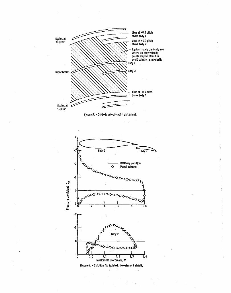
(2) A s1ngular1ty 1n the off-body velocity ca1culat10ns occurs when qn off-body p01nt 1~ .located at a d1stance of n*p1tch above or below a control po1nt located on an 1nput body (n = +1.+2 ••..• -1.-2 •... ). As the off-body p01nts approach th1s 10cat10n. errors w1ll develop 1n the ve10c1ty calculat10n. These errors can be av01ded by restr1ct1ng.the off-body p01nts to a reg10n wh1ch 1s w1th1n a tangent1al locat10n of plus or m1nus 0.9 * p1tch of the 1nput body 10cat10n as shown 1n f1gure 5.

Sample Input

A sample 1nput data set for a three~body problem (two cy11nders in a channel) 1s shown in Table I.. Labels for the various sect10ns of the 1nput have been 1nserted between the 1nput data l1nes. The 1nput l1nes that make up the actual data set have been appended w1th 1tem numbers wh1ch correspond w1th the descr1pt1ons g1ven prev1ously.

OUTPUT FILE DESCRIPTION

The output that 1s generated by the mult1ple-body-panel code 1s controlled by Item 14 1n the bas1c 1nput f1le. Two separate f1les may be generated. These are the l1st1ng or pr1nted output f11e of the tabulated flow solut10n. and an unformatted flow solut10n f1le. wh1ch 1s 1ntended for use w1th a post­processing graph1cs program.

output L1st1ng F11e

The code output l1st1ng file is sent to unit 06. wh1ch is the11ne pr1nter on most computer systems. It 1s a formatted data set. If the max1mum amount of output 1s requested by sett1ng lOUT = 3 in the basic input file (Item 14). the follow1ng information appears on the l1st1ng 1n the order given below:

(1) Labelled echo check of basic 1nput f1le.

(2) Transformed and physical blade shape geometry plus any blade shape generator tode d1agnost1cs. Listed for each body.

(3) Code-generated solution diagnostics.

(4) Transformed veloc1ty solut10n and singularity strengths for each body.

(5) Compress1ble-flow-solut1on 11st1ng and aux11ary-flow-solut10n output for each body.

11

(6) Off-body (flow-f1eld) veloc1ty-calculat1on'results.

For mult1ple-flow-case runs (NC5 > 1, Item 1 1n bas1c 1nput f1le), Items.3 to 6 are repeated for each add1t1onal flow case. The solut1on generates the output l1st1ng at var10us stages 1n the calculat1on. Th1s allows the user to rece1ve echo check and blade geometry even though the flow solut1on fa1ls.

Graph1cs F1le

50lut1on 1nformat1on. wh1ch can be used 1n a user-generated graph1cs code, 1s sent to un1t 60 by the code. The graph1cs f1le 1s generated 1f IPLOT = 1 1n Item 14 of the bas1c 1nput f1le. It 1s an unformatted data set. The f1le conta1ns the follow1ng 1nformat1on 1n the order g1ven below:

(1) The number of bod1es 1n the calculat10n (NBOOY 1n Item 1 bas1c 1nput f1le), the number of flow cases 1n the run (NC5 1n Item 1 bas1c 1nput f1le), the number of the body w1th the largest mer1d1onal coord1nate (bod1es are num­bered accord1ng to the order of the1r 1nput 1n the 1nput f1le), the number of the body w1th the smallest mer1d1ona1 coord1nate, the mean-flow-ca1culat1on control parameter (IMN 1n Item 1 bas1c 1nput f1le), the number of po1nts used to descr1be the mean flow (NMN 1n Item 1 bas1c 1nput f1le), cascade p1tch (5 1n Item 13 bas1c 1nput f1le), and the calculat10n reference length (REFLGT 1n Item 13 bas1c 1nput f1le).

(2) The number of elements used to descr1be each body (NELM 1n Item 10 bas1c 1nput f1le).

(3) Index of body coord1nate w1th the m1n1mum mer1d1onal value for each body. Index refers to the the locat1on of the po1nt 1n the coord1nate array as sent to th1s f1le.

(4) Index of body coord1nate w1th the max1mum mer1d1onal value for each body. Index refers to the the locat1on of the po1nt 1n the coord1nate array as sent to th1s f1le.

(5) The mer1d1onal coord1nate array of the body control po1nts where the surface veloc1t1es are calculated.

(6) The mer1d1onal coord1nate array of the panel/element end po1nts that make up the body.

(7) The tangent1al coord1nate array 1n rad1ans of the body control po1nts where the surface velocities are calculated.

(8) The tangent1al coordinate array 1n rad1ans of the panel/element end points that make up the body.

(9) Local transverse radius array at the panel end po1nts.

(10) The panel end point transformed mer1dional coordinate array.

Items (5) through (10) are repeated for each body as they are ordered 1n the input.

18

(11) Mer1d10nal coord1nate array for mean flow data (MRSP 1n Item 9 bas1c 1nput"flle).

(12) Transverse rad1us array at· mean-flow mer1d10nal coord1nates (RMSP 1n Item 9 bas1c 1nput f11e).

(13) stream sheet th1ckness array at mean-flow mer1d10nal coord1nates (BESP 1n Item 9 bas1c 1nput f11e).

~ \ .. . "

(14) Mean-flow cr1t1cal veloc1ty ~at10 array at the mean flow mer1d10nal coord1nates (E1ther calculated or g1ven 1n Item 9 bas1c 1nput f1le).

(15) Ind~x of the body control-p01nt coord1nate wh1ch marks the stagnat10n p01nt on the body. Index refers to the the 10cat10n of the p01nt 1n the body coord1nate array as sent to th1s f1le. If th1s 1ndex 1s ILU, then control p01nts ILU to NELM 11e on one s1de of the stagnat10n p01nt wh11e control p01nts ILU - 1 to 1 11e on the other s1de.

(16) D1stance along the body surface of th~ control p01nts from the lead1ng-edge stagnat10n p01nt.

(17) Local relat1ve cr1t1cal veloc1ty rat10 at the body control p01nts.

(18) Rat10 of local stat1c pressure to local relat1ve total pressure at the body control p01nts.

(19) Pressure coeff1c1ent at the body control p01nts. Reference dynam1c head 1s based on the upstream-stat10n relat1ve veloc1ty and dens1ty.

(20) Local relat1ve Mach number at the body control p01nts.

(21) Relat1ve stat1c pressure at body control p01nts.

(22) Relat1ve veloc1ty at body control p01nts.

Items (15) through (22) are repeated for each body.

(23) Upstream and downstream relat1ve veloc1ty of the mean flow.

(24) Number of off-body p01nts where the flow f1eld veloc1ty 1s to be calculated (Item lob 1n f1eld p01nt 1nput f11e).

(25) The transformed mer1d10nal coord1nate of the off-body p01nt, the tangent1al coord1nate for the off-body p01nt, the relat1ve veloc1ty at the off-body p01nt, and the flow angle 1n rad1ans w1th respect to the 1nput reference angle.

For the f1rst flow case, Items (24) and (25) are repeated for all the blocks of off-body p01nts g1ven 1n the f1eld-p01nt 1nput f11e. For all rema1n1ng flow cases, only the last block of off-body p01nts are wr1tten out. (See f1eld-p01nt 1nput f11e descr1pt10n for more 1nformat10n.)

(26) The 1nteger value "9999" 1s written to mark the end of one flow case and the start of data for the next.

19

Items (14) to (26) are repeated for each flow case.

The graph1cs f1le 1s generated by wr1te statements 1n three subrout1nes. Items (1) to (13) are wr1tten out 1n the subrout1ne GEOOPT. Items (14) to (23) are wr1tten out 1n subrout1ne CMPOPT. Items (24) to (26) are wr1tten out 1n s~brout1ne OFFBOD. If the user plans to use th1s f1le, he should look at these wr1te statements 1n order to get a better 1dea of how togo about read1ng in the 1nformat10n 1n the f1le.

TEST CASES

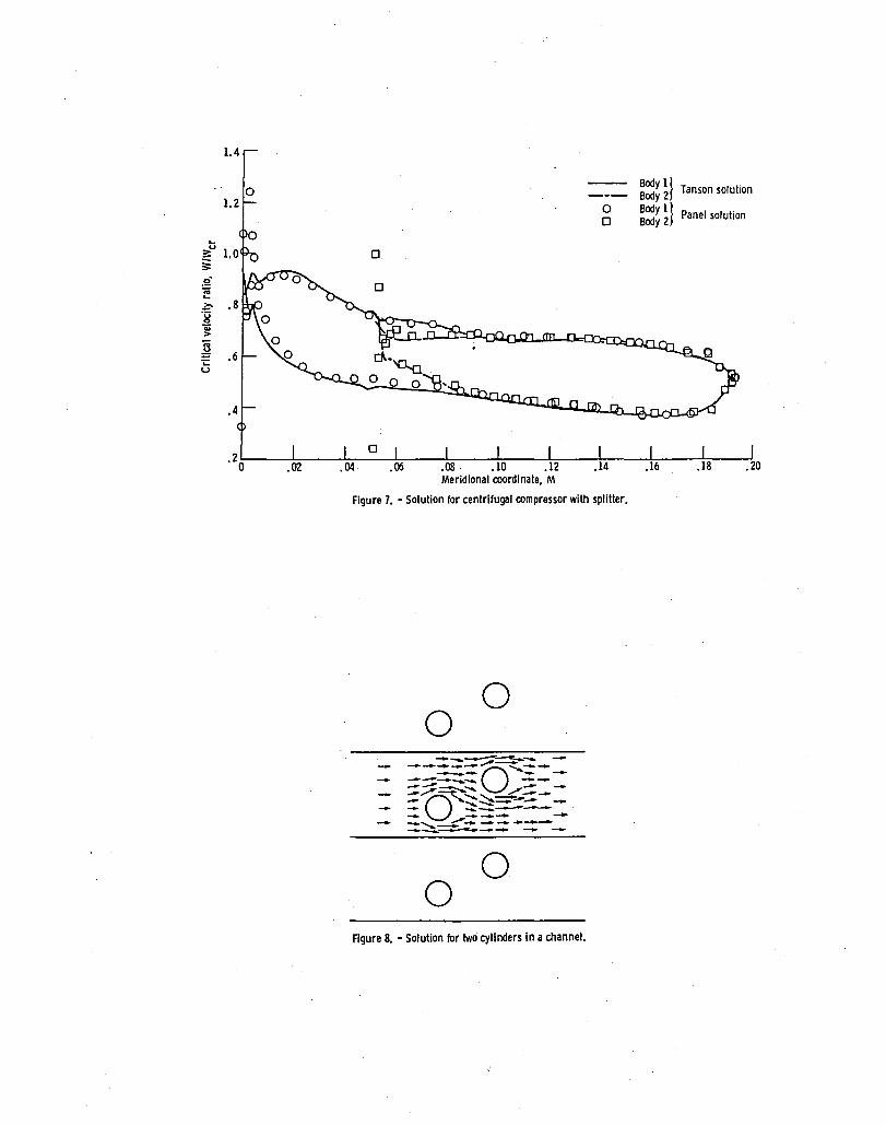
Three sample test-case input data sets accompany the code. The first case 1s an 1solated, two-element a1rfoil. The calculated surface-velocity distr1-but10n and geometry are given in f1gure 6, along with an exact solut10n by Williams (ref. 2). The second case 1s a centr1fuga1 compressor 1mpeller w1th sp11tter blade. F1gure 4 shows the problem geometry, and f1gure 7 shows the calculated surface veloc1ty. A flow solut10n from the f1n1te d1fference code TANSON (ref. 3) is also given on the figure. The f1na1 test case 1s a three­body problem of two cy11nders 1n a channel. The off-body-veloc1ty calculat10n capab111ty of the code was us~d to generate the vector plot of the solut10n flow field shown 1n f1gure 8.

20

REFERENCES

1. McFarland, t.R.: A Rap1d Blade-to~blade Solut1on.for Use 1n Turbomach1nery Des1gn. J. Eng. Gas Turb1nes Power, vol~ 106, no. 2, Apr. 1984, pp. 376-382.

2. Wil11ams, B.R .. An Exact Test Case for PlanePotentent1al Flow Abo4t Two Adjacent L1ft1ng Areof01ls. R.& M; No. 37l7 i Br1t1sh A.R.C., 1973.

3. Katsan1s, T.; and McNally, W.O.: 'FORTRAN Pro~ra~.·for Calculat1ng Veloc1-t1es and Stream11nes on a Blade~to~blade~StreamSurface of a Tandem Blade Turbomach1ne. NASA TN D-S044,196i ..

21

N N

TABLE I. - SAMPLE INPUT FILE. (ONLY LINES APPENDED WITH AN ITEM NUMBER ARE INCLUDED IN THE INPUT.)

BASIC INPUT FILE

INPUT DATA SET TITLE

INCOMPRESSIBLE FLOW THROUGH CYLINDERS - DENSITY = 2

CALCULATION CONTROL PARAMETERS

3 1 1 0 2

FLOW CONDITIONS

1000. 2. 2000. 10. O. O. O. 0.5 0.5 O.

MEAN FLOW PATH DESCRIPTION

-5. 1. 1.

7. 1. 1.

0

500.

FIRST BODY GEOMETRY DESCRIPTION (OPTION 2) - CHANNEL WALL (FLAT PLATE)

60 1 1 1 1

-3. -1. 0.01 0.01 O. 5. .-1. 0.01 .05 .5 1. 75 1.5 O. O. 2. O. O. o. O. O. O. 2. O. o • O. O.

SECOND BODY GEOMETRY DESCRIPTION (OPTION 1) - CYLINDER

40 0 0 0 (BLANK/DUMMY LINE)

0.500000 0.493840 0.475530 0.445500 0.404510 0.353550 0.293890 0.227000 0.154510 0.078220 0.000000 -0.078210 -0.154500 -0.226990 -0.293890 -0.353550

-0.404500 -0.445500 -0.475520 -0.493840 -0.500000 -0.493850 -0.475530 -0.445510 -0.404520 -0.353570 -0.293910 -0.227010 -0.154530 -0.078240 -0.000020 0.078190

0.154490 0.226970 0.293870 0.353530 0.404490 0.445490 0.475520 0.493840 0.500000 0.000000 -0.078220-0.154510 -0.227000 -0.293890 -0.353550 -0.404510 -0.445500

-0.475530 -0.493840 -0.500000 -0.493840 -0.475530 -0.445510 -0.404510 -0.353560

ITEM 1

ITEM 2

ITEM 3 ITEM 4 ITEM 5 ITEM 6 ITEM 7 ITEM 8

ITEM 9A 9B 9C

ITEM 10 ITEM 11 ITEM 12A

12B 12C 12D 12E 12F 12G 12H 121

ITEM 10 ITEM 11 ITEM 12A

12A 12A 12A 12A 12A

ITEM 12B 12B

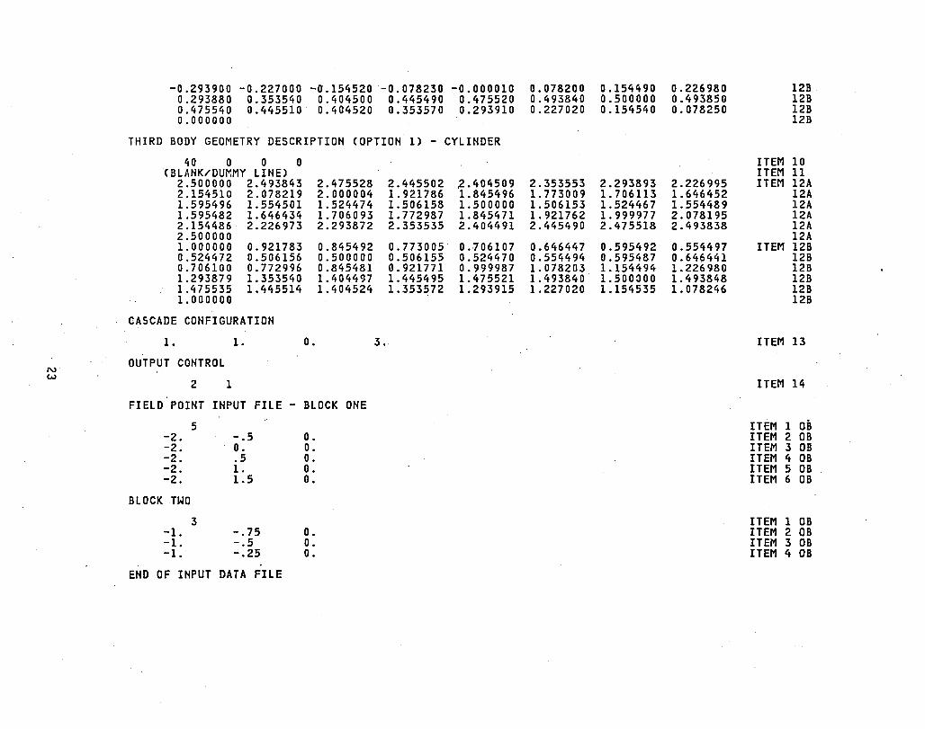
N w

-0.293900 -0.227000 -0.154520 -0.078230 -0.000010 0.293880 0.353540 0.404500 0.445490 0.475520 0.475540 0.445510 0.404520 0.353570 0.293910 0.000000

THIRD BODY GEOMETRY DESCRIPTION (OPTION 1) - CYLINDER

40 0 0 0 (BLANK/DUMMY LINE)

2.500000 2.493843 2.475528 2.154510 2.078219 2.000004 1.595496 1. 554501 1.524474 1.595482 1. 646434 1.706093 2.154486 2.226973 2.293872 2.500000 1.000000 0.921783 0.845492 0.524472 0.506156 0.500000 0.706100 0.772996 0.845481 1.293879 1.353540 1. 404497 1.475535 1.445514 1.404524 1.000000

CASCADE CONFIGURATION

1. 1. O.

OUTPUT CONTROL

2 1

FIELD POINT INPUT FILE - BLOCK ONE

-2. -2. -2. -2. -2.

BLOCK TWO

-1. -1. -1.

5

3

-.5 O. .5 1. 1.5

-.75 -.5 -.25

END OF INPUT DATA FILE

o. O. O. O. O.

o. O. O.

2.445502 ,2.404509 1.921786 1.845496 1.506158 1.500000 1.772987 1.845471 2.353535 2.404491

0.773005 0.706107 0.506155 0.524470 0.921771 0.999987 1. 445495 1.475521 1.353572 1.293915

3.

0.078200 0.154490 0.226980 12B 0.493840 0.500000 0.493850 12B 0.227020 0.154540 0.078250 12B

12B

ITEM 10 ITEM 11

2.353553 2.293893 2.226995 ITEM 12A 1. 773009 1.706113 1.646452 12A 1.506153 1.524467 1. 554489 12A 1. 921762 1.999977 2.078195 12A 2.445490 2.475518 2.493838 12A

12A 0.646447 0.595492 0.554497 ITEM 12B 0.554494 0.595487 0.646441 12B 1.078203 1.154494 1.226980 12B 1. 493840 1.500:100 1. 493848 12B 1.227020 1.154535 1. 078246 12B

12B

ITEM 13

ITEM 14

ITEM 1 OB ITEM 2 OB ITEM 3 OB ITEM 4 OB ITEM 5 OB ITEM 6 OB

ITEM 1 DB ITEM 2 DB ITEM 3 DB ITEM 4 DB

x:;. -:---;-- N 2 ",... MIN - I). PHIIN - I)

K+l. ~-~/·/rMIN). PHHN)

K K-l --~N , 1,

• Input point I .... MIl). PHIII) LM(2). PHII21

N-NELM+l

Meridional coordinate. M

Figure 1. - Blade shape input. option 1. IBLO - o .

MLE -I • ' Spline point

MTE

Meridional coordinate. M

Figure 2. - Blade shape Input, option 2,·IBLO -1.

o User's Input surface points • Leading edge elements, total number equals PL£ • NEIM • Upper surface elements, total number equals PUPS • (l - PL£). NEIM • Lower surface elements, total number equals [1 - PUPS • (l - PL£) - PLE1. NEIM • Trailing edge elements, total number equals 2 for blunt trailing edge

Braces indicate transition regions, element size controlled by FL£

~Braces indicate ~ transition regions,

element size controlled by FTE

Flgu re 3. - Output from blade generator, option 2. I BLD • 1.

1.5

!------Chord-------I

.5 1.0 Meridional coordinate, M

Figure 4. - Blade-row geometry Input parameters.

Bodies at +1 pitch

Input bodies

Bodies at -1 pitch

a. (,,)

'E Q)

'u E Q) 0 u Q) ...

. => VI VI Q) ...

Q..

-4

-1

0

-2

-1

line at -0.9 pitch below body 1

Figure 5. - Off-body velocity point placement.

c ~ -----B-od-y-l-----. ~

Williams solution o Panel solution

Or---~~~--------------~~---

1~ __ ~~ ____ L-____ L-____ L-__ ~

o 1.2 1.3 1.4 Meridional coordinate, M

Figure 6. - Solution for isolated, two-element airfoil.

1.4

0 Body I} Tanson solution

1.2 Body 2

0 Body 1 } Panel solution 0 Body 2

... u ::

i .2-., ... .t:-0g Cii >

~ .6 U

.4

.20

Figure 7. - Solution for centrifugal compressor with splitter.

o o

o o Figure 8. - Solution for two cylinders in a channel.

1. Report No. 2. Government Accession No.

NASA TM-87104 4. Title and Subtitle

A FORTRAN Computer Code for Calculat1ng Flows 1n Mult1ple-Blade-Element Cascades

7. Author(s)

Er1c R. McFarland

9. Performing Organization Name and Address

Nat10nal Aeronaut1cs ~ndSpace Adm1n1strat1on Lew1s Research Center Cleveland, Oh10 44135

12. Sponsoring Agency Name and Address

Nat10nal Aeronaut1cs and Space Administrat10n Wash1ngton, D.C. 20546

15. Supplementary Notes

Computer code ava1lable from COSMIC, Atlanta, Georg1a.

16. Abstract

3. Recipient's Catalog No.

5. Report Date

November 1985 6. Performing Organization Code

505-31-04 8. Performing Organization Report No.

E-2701 ~1-0.-W-o-rk-U-n-It-N-o.-------------------

11. Contract or Grant No.

13. Type of Report and Period Covered

Techn1cal Memorandum

14. Sponsoring Agency Code

A solut1on techn1que has been developed for solv1ng the mult1ple-blade-element, surface-of-revolut1on, blade-to-blade flow problem 1n turbomach1nery. The calcu­lat10n solves approx1mate flow equat10ns wh1ch 1nclude the effects of compress1-b1l1ty, rad1us change, blade-row rotat1on, and var1able stream sheet thickness. An 1ntegral equat10n solut1on <1.e., panel method) 1s used to solve the equa­t1ons. A descr1pt1on of the computer code and computer code 1nput 1s g1ven 1n th1 s report.

17. Key Words (Suggested by Author(s))

Turbomach1nery; Mult1ple body; Cascade flow; Blade-to-blade flow

18. Distribution Statement

Unclass1f1ed - un11m1ted STAR Category 02

19. Security Classlf. (of this report)

Unclassif1ed 20. Security Classif. (of this page)

Unc 1 ass if1 ed 21. No. of pages

·For sale by the National Technical Information Service, Springfield, Virginia 22161

22. Price·

End of Document