Department of Physics, Chemistry and Biology

Master’s Thesis

A first-principles non-equilibrium molecular dynamics

study of oxygen diffusion in Sm-doped ceria

Johan Klarbring

Linköping, 2015

LITH-IFM-A-EX--15/3093—SE

Department of Physics, Chemistry and Biology

Linköpings universitet, SE-581 83 Linköping, Sweden

Department of Physics, Chemistry and Biology

A first-principles non-equilibrium molecular dynamics

study of oxygen diffusion in Sm-doped ceria

Johan Klarbring

Linköping, 2015

Supervisor

Olga Vekilova Royal Institute of Technology (KTH)

Examiner

Sergei Simak IFM, Linköpings universitet

Datum

Date

2015-06-02

Department of Physics, Chemistry and Biology

Linköping University

URL för elektronisk version

http://www.ep.liu.se/

ISBN

ISRN: LITH-IFM-A-EX--15/3093--SE _________________________________________________________________

Serietitel och serienummer ISSN Title of series, numbering ______________________________

Språk Language

Svenska/Swedish Engelska/English

________________

Rapporttyp Report category

Licentiatavhandling Examensarbete

C-uppsats

D-uppsatsÖvrig rapport

_____________

Titel

Title A first-principles non-equilibrium molecular dynamics study of oxygen diffusion in Sm-doped ceria.

Författare Johan Klarbring Author

Nyckelord

Keyword density functional theory, non-equilibrium molecular dynamics, color diffusion, Sm-doped ceria, CeO2, ionic conductivity,

solid oxide fuel cells

Sammanfattning

Abstract

Solid oxide fuel cells are considered as one of the main alternatives for future sources of clean energy. To further improve their

performance, theoretical methods able to describe the diffusion process in candidate electrolyte materials at finite temperatures are needed. The method of choice for simulating systems at finite temperature is molecular dynamics. However, if the forces are

calculated directly from the Schrödinger equation (first-principles molecular dynamics) the computational expense is too high to

allow long enough simulations to properly capture the diffusion process in most materials.

This thesis introduces a method to deal with this problem using an external force field to speed up the diffusion process in the

simulation. The method is applied to study the diffusion of oxygen ions in Sm-doped ceria, which has showed promise in its use

as an electrolyte. Good agreement with experimental data is demonstrated, indicating high potential for future applications of

the method.

Abstract

Solid oxide fuel cells are considered as one of the main alternatives for fu-ture sources of clean energy. To further improve their performance, the-oretical methods able to describe the diffusion process in candidate elec-trolyte materials at finite temperatures are needed. The method of choicefor simulating systems at finite temperature is molecular dynamics. How-ever, if the forces are calculated directly from the Schrodinger equation(first-principles molecular dynamics) the computational expense is too highto allow long enough simulations to properly capture the diffusion processin most materials.

This thesis introduces a method to deal with this problem using an ex-ternal force field to speed up the diffusion process in the simulation. Themethod is applied to study the diffusion of oxygen ions in Sm-doped ce-ria, which has showed promise in its use as an electrolyte. Good agreementwith experimental data is demonstrated, indicating high potential for fu-ture applications of the method.

i

Acknowledgments

I would, first and foremost, like to thank my examiner, Sergei Simak, foralways being very encouraging and helpful, and for being very enjoyable tobe around. I also want to thank my supervisor, Olga Vekilova, for manyinteresting discussions and for being very helpful and supportive.

Johan KlarbringJune, 2015

ii

Contents

1 Introduction and Background 1

2 Theoretical Background 5

2.1 First-principles materials modeling . . . . . . . . . . . . . . . 5

2.1.1 The Schrodinger equation . . . . . . . . . . . . . . . . 6

2.1.2 The Born-Oppenheimer approximation . . . . . . . . . 7

2.2 Density functional theory . . . . . . . . . . . . . . . . . . . . . 8

2.2.1 Kohn-Sham DFT . . . . . . . . . . . . . . . . . . . . . 10

2.2.2 The Exchange-Correlation functional . . . . . . . . . . 12

2.2.3 Notes on spin . . . . . . . . . . . . . . . . . . . . . . . 14

2.3 Periodic Solids: the Bloch Theorem, k-points and Brillouinzone sampling . . . . . . . . . . . . . . . . . . . . . . . . . . . 15

2.4 Pseudopotentials and the Projector-augmented wave method. 16

2.5 Classical Statistical Mechanics . . . . . . . . . . . . . . . . . . 17

2.5.1 Ensembles, Phase Space and Distribution functions . . 17

2.5.2 Molecular Dynamics . . . . . . . . . . . . . . . . . . . 18

2.5.3 Linear Response Theory and Non-Equilibrium Molec-ular Dynamics . . . . . . . . . . . . . . . . . . . . . . . 20

iii

2.5.4 The Color Diffusion Algorithm . . . . . . . . . . . . . . 21

3 The Vienna ab-initio simulation package 24

4 Model system: ceria 26

4.1 Structure . . . . . . . . . . . . . . . . . . . . . . . . . . . . . 27

4.2 Doping and Ionic Conductivity . . . . . . . . . . . . . . . . . 27

4.3 Modeling ceria using DFT. . . . . . . . . . . . . . . . . . . . . 28

5 Methodological development 29

5.1 Implementing the color diffusion algorithm . . . . . . . . . . . 29

5.1.1 Controlling the temperature . . . . . . . . . . . . . . . 29

5.1.2 Choosing the Color Charge Distribution and the Ex-ternal Field Direction . . . . . . . . . . . . . . . . . . . 31

5.2 Technical details in the implementation . . . . . . . . . . . . . 35

5.2.1 Thermostat: Implementation and evaluation . . . . . . 35

5.2.2 Calculating the steady state color flux . . . . . . . . . 36

5.2.3 Choosing the strength of the external field: The lin-ear regime . . . . . . . . . . . . . . . . . . . . . . . . . 40

5.2.4 Identifying the vacancies . . . . . . . . . . . . . . . . . 41

5.3 Simulation setup and procedure . . . . . . . . . . . . . . . . . 42

6 Results and Discussion 46

6.1 Results . . . . . . . . . . . . . . . . . . . . . . . . . . . . . . . 46

6.1.1 Ionic conductivity . . . . . . . . . . . . . . . . . . . . . 46

6.1.2 Microscopic details of the diffusion process . . . . . . . 49

iv

6.2 Discussion . . . . . . . . . . . . . . . . . . . . . . . . . . . . . 51

6.2.1 Temperature dependence of the linear regime . . . . . 51

6.2.2 Comparison with other models . . . . . . . . . . . . . . 52

6.2.3 The correctional force . . . . . . . . . . . . . . . . . . 53

6.2.4 Temperature considerations . . . . . . . . . . . . . . . 55

7 Conclusions and Outlook 58

7.1 Future work . . . . . . . . . . . . . . . . . . . . . . . . . . . . 59

7.1.1 Methodological development . . . . . . . . . . . . . . . 59

7.1.2 Applications . . . . . . . . . . . . . . . . . . . . . . . . 60

Appendix A Matlab scripts 61

v

Chapter 1

Introduction and Background

Diffusion is a very intuitive phenomena when it occurs in a gas or a liquid.The scent from a cloud of perfume spreading throughout a room and milkdissolving in coffee are examples of diffusion process encountered in every-day life. Diffusion does, however, also occur in solids, which is what hasbeen the focus of the diploma work described in this thesis. A solid is anordered structure in which atoms oscillate around fixed lattice sites. Solidstate diffusion then occurs when an atom changes its position, either to avacant neighboring lattice site or to an interstitial position. Such an eventwill be referred to as a diffusive event or, simply, a jump.

Diffusion in solids is a very important phenomena to study from a techno-logical point of view. Examples of applications are diffusion bonding, steelhardening, oxygen sensors, and fuel cells. This last example is going to begiven some attention in this thesis.

There is a great need for clean and efficient energy-conversion devices intoday’s society. One promising candidate is the solid oxide fuel cell (SOFC)[1]. Figure 1.1 schematically shows the operating procedure of a SOFC:Oxygen ions move through the solid electrolyte and react with the hydro-gen injected on the anode side yielding water and spare electrons which aredirected through a circuit and can perform work. As long as the hydrogenfuel can be cleanly produced, the only waste from the fuel cell being water,the energy conversion in a SOFC is a very clean process.

The rate of the ionic conduction through the electrolyte is very importantfor the performance of the fuel cell. This rate is directly related to the dif-

1

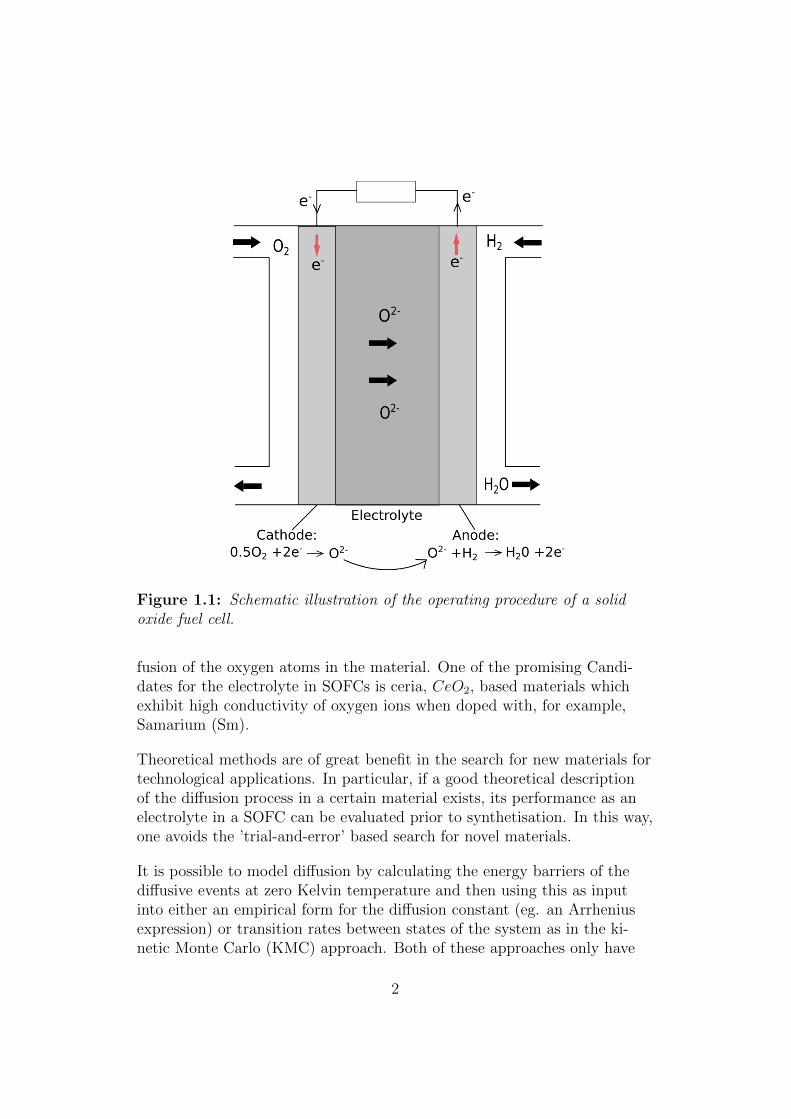
Figure 1.1: Schematic illustration of the operating procedure of a solidoxide fuel cell.

fusion of the oxygen atoms in the material. One of the promising Candi-dates for the electrolyte in SOFCs is ceria, CeO2, based materials whichexhibit high conductivity of oxygen ions when doped with, for example,Samarium (Sm).

Theoretical methods are of great benefit in the search for new materials fortechnological applications. In particular, if a good theoretical descriptionof the diffusion process in a certain material exists, its performance as anelectrolyte in a SOFC can be evaluated prior to synthetisation. In this way,one avoids the ’trial-and-error’ based search for novel materials.

It is possible to model diffusion by calculating the energy barriers of thediffusive events at zero Kelvin temperature and then using this as inputinto either an empirical form for the diffusion constant (eg. an Arrheniusexpression) or transition rates between states of the system as in the ki-netic Monte Carlo (KMC) approach. Both of these approaches only have

2

implicit treatments of finite temperature effects. This may be adequate fordescribing processes occurring at up to room temperature. Many of thetechnological applications of solid state diffusion, however, take place atmuch higher temperatures. As an example the operating temperature of aSOFC lies in the range 700 - 1200 K, where we expect temperature effectsto be of great importance.

The method of choice for explicitly treating temperature effects is molec-ular dynamics (MD) in which the movement of the atoms in the system issimulated in time by numerically solving the appropriate equations of mo-tion. MD methods can naturally be divided into two types: one in whichthe interactions between atoms in the system are fitted to some empiricaldata and the other where they are calculated from first-principles.

In the first-principles, or ab-initio, approach the interactions are based di-rectly on the laws of quantum mechanics (QM) and any empirical data oradjustable parameters are avoided. In practice using this type of an ap-proach requires the use of a number of approximations for all but the mostsimple systems. These approximations, however, are based on physical ar-guments and are not performed in a way to try to match empirical data1.

The strength of this approach, which we will refer to as ab-initio MD (AIMD),lies mainly in its universality. The method can be used to study any mate-rial, as long as it is within the realm of applicability of the approximationsused. The main drawback is the extreme computational complexity. Evenusing today’s high performing supercomputers it is only possible to simu-late the movement of a few hundred atoms for times ranging up to maxi-mally nanoseconds.

While this time limit may be enough to simulate the diffusion process in aliquid, in most cases the diffusion rate in a solid is many orders of magni-tude slower and we simply cannot perform long enough calculations to geta proper description of the diffusion process. One can then either turn toan empirical description of the interactions or use, for example, KMC, bothof which may severely limit the accuracy and the range of applicability.

An exciting way of dealing with the ”time scale” problem of modeling solidstate diffusion by AIMD was recently proposed by Aeberhard et al. [2].They use an non-equilibrium MD (NEMD) approach where they apply an

1While the approximations are not based on empirical data, it is very important toverify the results w.r.t empirical data.

3

external field to the system. More precisely they apply a version of thecolor-diffusion algorithm, originally proposed by Evans et al. [3] to studydiffusion in liquids.

In the NEMD approach one adds an external force to the equations of mo-tion. If the response of the system to this field is linear the dynamics, andthus the diffusion process, are accelerated but remain qualitatively realistic.In this way one can model diffusion in much shorter simulation times thanin equilibrium AIMD.

This thesis outlines a first-principles NEMD approached based on the den-sity functional theory (DFT) for describing solid state diffusion. It is di-rectly validated by comparison of the obtained ionic conductivity of Smdoped ceria (SDC) to experimental values from the literature. The goodagreement indicates that this method can be used to further study the dif-fusion process in ceria and other materials, and can thus, for example, beof use in the development of more effective SOFCs.

4

Chapter 2

Theoretical Background

This chapter gives brief descriptions of the different theoretical methodsused in this diploma work. The material can be divided into two sections,one on first-principles modeling, in particular the density functional theory(DFT) and the other on classical statistical mechanics. The first sectionis mainly based on the books by Martin [4], Giustino [5] and Kohanoff [6]and the second section is primarily inspired by books by Evans and Morriss[7], Tuckerman [8] and Allen and Tildesley [9]. References are, wheneverpossible, also given to the original papers.

2.1 First-principles materials modeling

The approach used in this work is usually refereed to as first-principles orab-inito modelling, implying that we use a bottom-up approach, based onfundamental physical laws and work our way, by using valid approxima-tions, to a model where we can accurately describe desired properties ofmaterials.

Starting from the bottom, we model any piece of material as consisting ofnuclei and electrons, we thus ignore any effects originating from the smallerconstituents of the nuclei. We will also assume that relativistic effects arenegligible1. The theoretical framework of choice for this type of model is

1Although some effects, such as spin, that actually originate from a relativistic treat-ment will be briefly considered.

5

(non-relativistic) quantum mechanics (QM).

In the Schrodinger formulation of QM, the description of the state of aphysical system is completely contained in its wave function, Ψ(r, t), wherer and t represents all spatial and time dependence, respectively. The mostinformation about a physical property, A, we can extract from such a sys-tem is its expectation value,

〈A〉 = 〈Ψ|A|Ψ〉 =

∫Ψ∗AΨdr (2.1)

where A is the operator corresponding to the observable A and where we inthe middle equality have used a shorthand notation due to Dirac.

2.1.1 The Schrodinger equation

The time evolution of the wavefunction is given by the (time-dependent)Schrodinger equation

ih∂Ψ(r, t)

∂t= H(r, t)Ψ(r, t), (2.2)

where h is the reduced Planck constant and H is the Hamiltonian or totalenergy operator of the system. In the case of a time-independent Hamilto-nian, H(r, t) = H(r) ≡ H, the time and spatial dependence of the wave-function can be separated yielding the time-independent Schrodinger equa-tion

HΨ(r) = EΨ(r), (2.3)

which has the form of an eigenvalue equation. In the following we will referto Eq. (2.3) as just the Schrodinger equation (SE).

Pausing for a moment we note that the study of materials in our modelessentially consists of solving the SE (2.3) and then calculating the expec-tation value of whatever property we are interested in using Eq. (2.1).

Let us examine the complexity of such a task. As an example, take onecm3 of ceria, which contains around 7 · 1022 nuclei, and 2 · 1024 electrons.The corresponding wavefunction will then be a function of the position riof the electrons and positions RI of all the nuclei,

Ψ(r) = Ψ(r1, r2, ..., rn,R1,R2, ...,RN) = Ψ(ri,RI),

6

where n is of the order 1024 and N is of the order 1022, and the SE willthen be a second-order differential equation in something like 1024 vari-ables. It is clearly futile to attempt to solve this problem as it is. We willinstead invoke a series of approximations which make the problem feasible.

2.1.2 The Born-Oppenheimer approximation

The Hamiltonian operator of our system in atomic units looks as follows

H = −1

2

n∑i=1

∇2i−

1

2MI

N∑I=1

∇2I+∑i>j

1

|ri − rj|+∑I>J

1

|RI −RJ |−∑i,I

1

|RI − ri|,

(2.4)where lower and upper case indices refer to electrons and nuclei, respec-tively, MI is the mass of nuclei I and n and N are the number of electronsand nuclei, respectively. The terms in Eq. 2.4 correspond, in order, to theelectronic kinetic energy Te, the nuclear kinetic energy Tn, the electron-electron and nuclear-nuclear repulsion Vee and Vnn and the electron-nuclearattraction Ven.The SE then takes the form,

(Te + Tn + Vee + Vne + Vnn)Ψ = EΨ. (2.5)

Now, the ratio of the electron and proton/neutron mass is around 1:2000,this means that the mass of the nuclei and the electrons will differ by morethan 4 orders of magnitude. We can thus expect the movements of theelectrons and the nuclei to take place on completely different timescales;the electrons move much faster than the nuclei. A reasonable approxima-tion would then seem to be that we can separate the movement of the two.This leads us to the ansatz,

Ψ(ri,RI) = ψ(ri : RI)χ(RI), (2.6)

where the notation ψ(ri : RI) indicates a parametrical dependence on thenuclear positions RI , and where we assume that ψ(ri : RI) is the groundstate solution of the electronic SE,

Heψ(ri : RI) = E0(RI)ψ(ri : RI), (2.7)

with He ≡ Te + Vee + Vne.2 What we are implicitly assuming now is that

the electrons stay in their ground state when the nuclei move; The elec-

2We, of course, do not know that this ansatz is valid. What we can always do, how-ever, is to write the full wavefunction Ψ(ri,RI) =

∑i χ(R)ψi(ri : RI), where ψi are all

the eigenfunctions of the electronic Hamiltonian, and proceed from there.

7

trons move so fast compared to the nuclei that they can be considered toinstantly be in their ground state during the movement of the nuclei.

Insertion of the ansatz (2.6) into the SE (2.5) yields,

(He + Tn + Vnn)ψ(ri : RI)χ(RI) = (E0(RI) + Tn + Vnn)ψ(ri : RI)χ(RI)

= Eψ(ri : RI)χ(RI)(2.8)

If we also take ψ to be normalized,∫ψ∗ψdr = 1, we can multiply the equa-

tion above by ψ∗ and integrate over the electron coordinates to get,

(Tn + Vnn + E0(RI))χ(RI) = Eχ(RI). (2.9)

The full SE (2.5) has now been separated into an electronic SE (2.7) and aSE for the nuclei Eq. (2.9).

The Classical Nuclei approximation and Born-Oppenheimer Molec-ular Dynamics

Except for some of the most light elements the quantum effects of the nu-clei can, to a good approximation, be neglected and they can thus be treatedas classical point particles. One can show [6] that taking the classical h →0 limit of Eq. (2.9) gives the following classical equations of motion for thenuclei,

MId2RI

dt2= −∇IU(RI), (2.10)

where,

U(RI) = E0(RI) +∑J>I

1

|RI −RJ |. (2.11)

If we assume that we can solve the electronic SE (2.7), the movement ofthe nuclei can then be extracted by applying the standard molecular dy-namics (MD) techniques of section 2.5.2 to Eq. (2.10). This is what isknown as Born-Oppenheimer Molecular Dynamics (BOMD).

2.2 Density functional theory

After applying the approximations of the previous section we are still leftwith the hard task of solving the electronic SE (2.7) for the ground stateenergy E0. This problem will be considered within the framework of DFT.

8

Since we now are only dealing explicitly with electrons, a natural quantityto consider is the elecron density at position r, ρ(r). The electrons do nothave well defined positions so the best we can do is to consider the prob-ability that a certain electron is at a certain position r. If we consider asystem of n electrons, the probability that electron 1 is at position r whilethe other electrons are allowed to be anywhere else is

P1(r) =

∫|ψ(r, r2, ..., rn)|2dr2...drn. (2.12)

The electron density at position r is then given by

ρ(r) = P1(r) + P2(r) + ...+ Pn(r). (2.13)

In QM the electrons are indistinguishable particles so it does not matterwhich electron we leave out of the integration in Eq. (2.12), and we mustthus have P1(r) = P2(r) = ... = Pn(r), so finally,

ρ(r) = n

∫|ψ(r, r2, ..., rn)|2dr2...drn. (2.14)

The natural question to ask now is what information we can extract fromknowing only the electron density. It turns out that the answer is: essen-tially all possible information. This fact is the content of the Hohenberg-Kohn (HK) theorems [10]

The first HK theorem

A general form of the Hamiltonian of a system of electrons moving in someexternal potential is,

He = −1

2

n∑i=1

∇2i +

∑i>j

1

|ri − rj|+

n∑i=1

Vext(ri), (2.15)

where Vext could, for example, represent the electron-nuclear attractionat fixed nuclear positions. The first Hohenberg-Kohn theorem states thatgiven an electron density ρ(r), the external potential in the above equationis uniquely determined. From this it follows that the electronic Hamilto-nian is also completely determined by ρ(r) and thus any possible informa-tion about the system can be extracted by means of solving the full SEwith this Hamiltonian.

9

The second HK theorem

The statement of the second HK theorem will seem almost obvious at thispoint. Since by the first HK theorem above all properties of the system canbe determined by knowing only the electron density it seems natural thatwe can write the energy as a functional of the electron density, and thatthe ground state energy is obtained by minimizing this functional over theelectron densities that corresponds to the right number of electrons in oursystem:

E0 = minρ(r)

E[ρ(r)] subject to

∫ρ(r)dr = n, (2.16)

where n is the number of electrons in our system and the ground state den-sity, ρ(r) is the one corresponding to the minimization of the energy above.

To summarize, the HK theorems tells us that ρ(r) contains all possible in-formation about the state of the system and that we find the ground stateelectron density and ground state energy by minimizing some functional ofthe electron density. They do not, however, give any hint to how this func-tional may look.

2.2.1 Kohn-Sham DFT

In the Kohn-Sham (KS) [11] approach to DFT one assumes that the groundstate density can be written as the density of a system of non-interactingelectrons, described by the KS-orbitals, φi(r), i = 1, ...., n, i.e.,

ρ(r) =n∑i=1

|φi(r)|2 . (2.17)

One then writes the energy functional of (2.16) as

EKS[ρ] = TKS[ρ] + EHartree[ρ] + Eext[ρ] + EXC [ρ], (2.18)

where TKS[ρ] is the kinetic energy of the non-interacting electrons,

EHartree[ρ] =1

2

∫∫ρ(r)ρ(r′)

|r− r′|drdr′ (2.19)

is the classical energy of an electron gas of density ρ(r),

Eext[ρ] = 〈Ψ|Vext|Ψ〉 =

∫Vext(r)ρ(r)dr (2.20)

10

is the energy resulting from the external potential (in particular from thenuclear-electron attraction), and EXC [ρ] is known as the exchange-correlation(XC) energy, which contains whatever missing in the first 3 terms to makeEKS[ρ] equal to the real ground-state energy, E0.

Following the second HK theorem, the next step is to minimize EKS[ρ]w.r.t ρ(r), under the requirement that ρ(r) integrates to n. This is achievedby introducing the Lagrangian,

Λ = EKS[ρ]− λ(∫

ρ(r)dr− n)

(2.21)

where λ is the Lagrange-multiplier and requiring its functional derivativew.r.t. ρ to be zero:

δΛ

δρ= 0. (2.22)

One can then show that this will lead to a set of n Schrodinger-like equa-tions for the orbitals φi

HKSφi = εiφi, (2.23)

which are known as the Kohn-Sham equations. Here HKS is the Kohn-Sham Hamiltonian,

HKS = −1

2∇2 + Vext(r) +

∫ρ(r′)

|r− r′|dr′ +

δEXC [ρ]

δρ(r),

= −1

2∇2 + Vext(r) + VHartree(r) + VXC(r),

= −1

2∇2 + VKS(r),

(2.24)

where we have defined the Hartree potential VHartree and the XC-potentialVXC .

Formally, we have now replaced the problem of solving the electronic SEEq. (2.7), for the many-body wavefunction Ψ, with solving n Schrodinger-like equations for independent electrons moving in the effective potentialVKS. Computationally this amounts to replacing one 2nd order differen-tial equation in 3n variables, with n 2nd order differential equations in 3variables, which is certainly preferable.

In practice Eqs. (2.17), (2.23) and (2.24) are solved self-consistently, mean-ing that we first guess an initial density, ρ1(r), this gives us VKS[ρ1] usingEq. (2.24), from which we solve the KS equations (2.23) for the orbitals

11

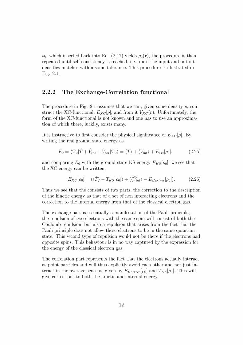
φi, which inserted back into Eq. (2.17) yields ρ2(r), the procedure is thenrepeated until self-consistency is reached, i.e., until the input and outputdensities matches within some tolerance. This procedure is illustrated inFig. 2.1.

2.2.2 The Exchange-Correlation functional

The procedure in Fig. 2.1 assumes that we can, given some density ρ, con-struct the XC-functional, EXC [ρ], and from it VXC(r). Unfortunately, theform of the XC-functional is not known and one has to use an approxima-tion of which there, luckily, exists many.

It is instructive to first consider the physical significance of EXC [ρ]. Bywriting the real ground state energy as

E0 = 〈Ψ0|T + Vint + Vext|Ψ0〉 = 〈T 〉+ 〈Vint〉+ Eext[ρ0]. (2.25)

and comparing E0 with the ground state KS energy EKS[ρ0], we see thatthe XC-energy can be written,

EXC [ρ0] = (〈T 〉 − TKS[ρ0]) + (〈Vint〉 − EHartree[ρ0]). (2.26)

Thus we see that the consists of two parts, the correction to the descriptionof the kinetic energy as that of a set of non interacting electrons and thecorrection to the internal energy from that of the classical electron gas.

The exchange part is essentially a manifestation of the Pauli principle;the repulsion of two electrons with the same spin will consist of both theCoulomb repulsion, but also a repulsion that arises from the fact that thePauli principle does not allow these electrons to be in the same quantumstate. This second type of repulsion would not be there if the electrons hadopposite spins. This behaviour is in no way captured by the expression forthe energy of the classical electron gas.

The correlation part represents the fact that the electrons actually interactas point particles and will thus explicitly avoid each other and not just in-teract in the average sense as given by EHartree[ρ0] and TKS[ρ0]. This willgive corrections to both the kinetic and internal energy.

12

Initial guess: ρin(r)

VKS(r) = Vext(r) +∫ ρ(r′)|r−r′|dr

′ + δEXC [ρ]δρ(r)

Solve the KS-equations:(−1

2∇2 + VKS(r)

)φi = εiφi

New density:ρout(r) =

∑ni=1 |φi(r)|2

Self consistency?:”ρout = ρin”?

Update density:”ρin → ρout”

Done!ρout = ρ0

E0 = EKS[ρout]

no

yes

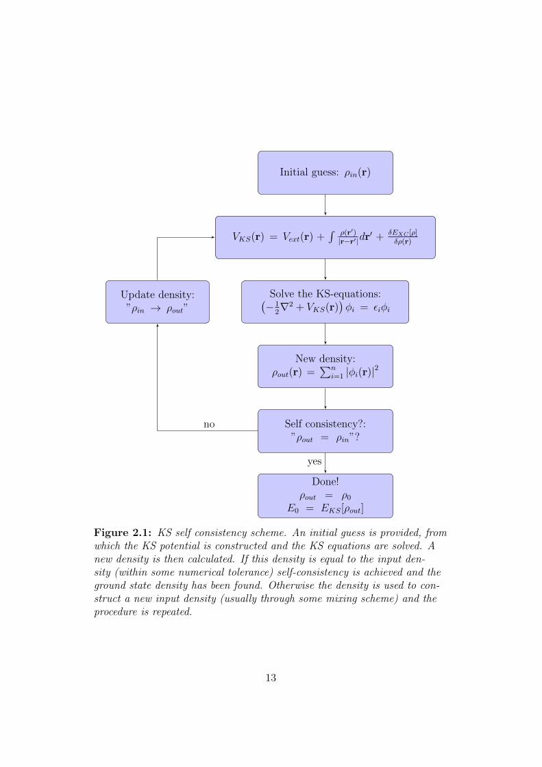
Figure 2.1: KS self consistency scheme. An initial guess is provided, fromwhich the KS potential is constructed and the KS equations are solved. Anew density is then calculated. If this density is equal to the input den-sity (within some numerical tolerance) self-consistency is achieved and theground state density has been found. Otherwise the density is used to con-struct a new input density (usually through some mixing scheme) and theprocedure is repeated.

13

The Local Density Approximation (LDA)

Looking at the expression of the XC-functional in Eq. (2.26) and the con-siderations that followed, the corrections to TKS and EHartree would seemto be largely short ranged. If this is the case, the XC-energy can be ap-proximated as a local functional of ρ. In the local density approximation(LDA) the XC-functional is written as

ELDAXC [ρ] =

∫ρ(r)εhomXC (ρ(r))dr, (2.27)

where εhomXC (ρ(r)) is the exchange correlation per-particle of a homogeneouselectron gas of density ρ, i.e. at each point we consider the XC-energy tobe described by that of a homogeneous electron gas with the density in thispoint.

εhomXC is then usually written as a sum of an exchange part, εhomX and a cor-relation part εhomC . An exact expression for the exchange part can be found,and the correlation part is usually parametrised using data from quantumMonte Carlo calculations first performed by Ceperley and Alder [12].

Generalised Gradient Approximations (GGA)

Naturally, the next step in improving the XC-functional is to include thegradient of the density in the expression, i.e.,

EGGAXC [ρ] =

∫ρ(r)εGGAXC (ρ(r),∇ρ(r))dr. (2.28)

These type of approximations to the XC-functional are known as gener-alised gradient approximations (GGAs). Many different GGAs exist, in thecalculations in this work we will use the form proposed by Perdew, Burkeand Ernzerhof [13].

2.2.3 Notes on spin

So far, we have not considered the impact of the spin of the electrons. Toextend the above theory to spin-polarized systems we write the density as asum of a spin up and a spin down density:

ρ(r) = ρ↓(r) + ρ↑(r). (2.29)

14

The XC-functional will then in general depend on both densities, i.e., EXC =EXC [ρ↓(r), ρ↑(r)], and one adds a spin-index, s =↑ / ↓, to the KS orbitals:φi → φsi . The densities are then given as

ρs(r) =ns∑i=1

|φsi (r)|2, (2.30)

where ns is the number of electrson with spin s.

2.3 Periodic Solids: the Bloch Theorem, k-points

and Brillouin zone sampling

The focus in this work is on bulk properties of solid materials. They aremodeled as periodic crystals, where a number of atoms in some unit cellis repeated periodically in all directions. In this model it seems reasonablethat we could solve the KS equations in only a small a part of the systemand then in some way use this periodicity to extend the solution to thewhole crystal.

In such a system the KS effective potential will be periodic VKS(r) = VKS(r+R), where R represents the periodicity of the crystal. The KS orbitals canthen be written

φ(k)j (r) = eik·ruj,k(r) (2.31)

where uj,k(r) = uj,k(r + R) and k are vectors in reciprocal (Fourier) space.This is the result of the Bloch theorem. The number of k-vectors that givesunique Bloch states in Eq. (2.31) are the same as the number of primi-tive unit cells in the crystal and are contained in the (first) Brillouin zone(BZ).

Using the Bloch theorem one can now3 express a quantity that is periodicin repetitions of the unit cell as an average over the BZ. In particular theelectron density ρ(r) can be expressed as

ρ(r) =∑k∈BZ

ωk

Ncell∑j=1

|φ(k)j (r)|2, (2.32)

3For details see, for example, Martin [4] Ch. 4 and Ch. 12 or Kohanoff [6] Ch. 6.

15

where where the index j now runs over all electrons in the unit cell, and kruns over all the k-points in the BZ and ωk is a weighting factor. In thisway one can, instead of solving n KS equations(2.23), where n is the num-ber of electrons in the whole crystal, solve the set of KS equations

HKSφ(k)j = ε

(k)j φ

(k)j , (2.33)

ρ(r) is then calculated from Eq. (2.32) and the procedure is repeated as inFig. 2.1.

If the crystal is modeled as infinitely large there will be an infinite numberof k-points in the BZ. In actual calculations one samples the BZ from a fi-nite number of, well chosen, k-points. How many points that are neededvaries drastically depending on the system, what property one wants tocalculate and the required accuracy. In some cases it is possible to getaway with using just a few points which, of course, highly reduces the com-putation time.

2.4 Pseudopotentials and the Projector-augmented

wave method.

Usually the electrons in a system of atoms can, to a good approximation,be divide into core- and valence-electrons. Where only the valence elec-trons are assumed to participate in the bonding of the system. One canthen introduce the concept of an ionic core consisting of both the nucleusand the core electrons of this atom, which are then treated independentlyof the environment of the atom and are said to be frozen in the core. Theeffective potential resulting from this ionic core is termed a pseudopotential.

Furthermore, the form of the wavefunctions of the valence electrons nearthe nucleus, which usually is of oscillating character, is normally of littleimportance to collective properties of the system. It is then reasonable toreplace the all-electron (AE) wavefunction4 with a pseudo wavefunctionwhich is equal to the all-electron wavefunction outside some core cutoff ra-dius, rc, but which is much smoother inside rc.

In the calculations in this work, we will use a plane wave expansion of theKS orbitals. In this case the pseudo wavefunction is particularly useful,

4Not the many-body wavefunction.

16

since the oscillating character of the AE wavefunction close to the corewould require a large number of plane wave components to be accuratelydescribed, while in the interstitial region between atoms much fewer com-ponents are needed.

In the projector augmented wave (PAW) method [14], the all-electron wave-function, φ, is recovered from the pseudo wavefunction, φ, through a lin-ear transformation which is equal to the identity transformation outsidespheres of radii rc centered at each atom. In Dirac notation,

|φ〉 = |φ〉+∑m

〈pm|φ〉(|φm〉 − |φm〉

)(2.34)

where φm is a set of pseudo partial-waves, which are equal to the AE partial-waves, φm, outside rc and pm is a set of projection operators satisfying〈pi|φj〉 = δi,j. The AE partial-waves are obtained from calculations on areference atom while the pseudo partial-waves are, for example5, expandedin terms of spherical Bessel functions inside rc [15].

2.5 Classical Statistical Mechanics

The classical nuclei approximation, resulting in Eq. (2.10), suggests thatwe can, in fact, use the framework of classical statistical mechanics to aidthe description of a system in which this approximation is valid.

2.5.1 Ensembles, Phase Space and Distribution functions

Central to statistical mechanics is the concept of an ensemble which wedefine to be a large (infinite) collection of systems with a common set ofmacroscopic properties described by the same microscopic particle inter-actions. Some examples of common ensembles are the micro-canonical(NV E-)ensemble defined by constant number of particles, volume and en-ergy, and the canonical (NV T -)ensemble where instead of the energy thetemperature is constant.

Time evolution in the ensemble picture consists of letting the members ofthe ensemble be given different microscopic initial conditions from which to

5This is the case in VASP, see section 3

17

evolve. Macroscopic properties (temperature, pressure, energy etc) are thenobtained by averaging over the ensemble members.

The microscopic state of a N particle system is completely determined byspecifying the (generalised) positions q = (q1, q2, ..., q3N) and (generalised)momenta p = (p1, p2, ..., p3N) of each particle. The 6N-dimensional spaceconsisting of all possible points x = (q,p) is called phase space.

To be able to calculate averages we introduce the (phase space) distributionfunction f(x, t) and define f(x, t)dx = f(x, t)dqdp to be the fraction ofthe accessible states of the system under study contained in the (hyper-)cube of volume dx in phase space centered around x. This allows us tocalculated the average value of a phase variable A(x) as

〈A〉 =

∫f(x, t)A(x)dx, (2.35)

where the integral is taken over all of phase space. The distribution func-tions of the micro canonical and canonical ensembles are, up to a constantnormalisation factor, given by

fNV E(x) = δ(H(x)− E), (2.36)

and,

fNV T (x) = exp

(−H(x)

kBT

), (2.37)

respectively. Here kB is the Boltzmann constant.

2.5.2 Molecular Dynamics

In the molecular dynamics (MD) method, instead of ensemble-averages,Eq. (2.35), one calculates time-averages in a single member of the ensem-ble, i.e.,

〈A〉t = limτ→∞

∫ τ

0

A(t)dt. (2.38)

One then proceeds under the assumption that time- and ensemble-averagingyields the same result. This is known as the ergodic-hypothesis.

Given the equations of motion (EOM) for the particles in a system the MDmethod then consists of the numerical integration of these EOM while cal-culating the value of some quantity at each time step of the integration. If

18

this procedure is carried out for a long enough time Eq. (2.38) can be usedto calculate the average of the quantity.

For a system with the classical Hamiltonian

H(r,p) =N∑i=1

p2i

2mi

+ U(r), (2.39)

where r and p are the positions and momenta of the system, respectively,the EOM are

ri =pimi

, (2.40a)

pi = Fi, (2.40b)

where Fi = −∇riU(r) is the force on particle i. A commonly used integra-tion scheme for these equations is the velocity Verlet algorithm

ri(t+ ∆t) = ri(t) + ∆tvi(t) +∆t2

2mi

Fi(t+ ∆t), (2.41a)

vi(t+ ∆t) = vi(t) +∆t2

2mi

(Fi(t) + Fi(t+ ∆t)) , (2.41b)

where ∆t is the integration time step. Thus, given initial positions and ve-locities and a way to calculate the force, Eqs. (2.41) can be used to ad-vance the system forward in time.

Eqs. (2.41) are easily obtained from Eqs. (2.40) and second order Taylorexpansions of r(t + ∆t) and can be straightforwardly generalised to handlemore complicated EOM.

Constant temperature MD. Thermostats

The total energy of a system evolving under Eqs. (2.40) will, if the numer-ical integration is accurate enough, be conserved. Often, however, it maybe more realistic to consider a system evolving under constant temperaturesince this may more closely mimic an experimental situation.

Conceptually, the simplest way to carry out constant temperature MD is todefine the instantaneous temperature, Tinst., as the temperature of an idealgas with the velocities of the particles in our system:

3

2kBTinst. =

N∑i=1

miv2i

2, (2.42)

19

where kB is the Boltzmann constant and mi and vi is the mass and veloc-ity of particle i, respectivey, and then scale all velocities in the system eachtime step to make Tinst. match a desired temperature [16], this is known asa velocity scaling (VS) thermostat.

A related, but more sophisticated, method is using the Gaussian isokineticthermostat [7], which incorporates a ”friction-like” term α into the EOM:

ri =pimi

, (2.43a)

pi = Fi − αpi, (2.43b)

α is then treated as a Lagrangian multiplier used to satisfy the constraint

g(pi) = Tinst.(pi)− T0 = 0, (2.44)

with Tinst.(pi) given by Eq. (2.42) and T0 the desired temperature.

If one uses the velocity Verlet integration scheme the Gaussian isokineticand the velocity scaling thermostats become equivalent in the limit ∆t →0 [17]. Inspired by this we symbolically represent the VS thermostat byinserting a friction term α in the EOM.

Perhaps the most commonly used way of performing constant temperatureMD is using the Nose, or Nose-Hoover, thermostat [18]. This method isbased on an extended phase-space, where one introduces two extra degreesof freedom, s and ps, representing the thermostat. The extended phasespace is then (q,p, s, ps) for which one writes down a Hamiltonian andshows that performing constant energy molecular dynamics (using Hamil-tons eqs.) in the extended system (q,p, s, ps) will yield constant tempera-ture in the physical system (q,p).

2.5.3 Linear Response Theory and Non-Equilibrium Molec-ular Dynamics

We will now investigate the effect of adding an external force to a systemdescribed by the EOM (2.40). The relevant EOM are [8, 7],

ri =pimi

+ CiFe, (2.45a)

pi = Fi + DiFe, (2.45b)

20

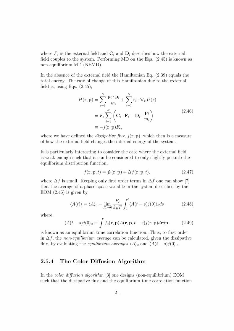
where Fe is the external field and Ci and Di describes how the externalfield couples to the system. Performing MD on the Eqs. (2.45) is known asnon-equilibrium MD (NEMD).

In the absence of the external field the Hamiltonian Eq. (2.39) equals thetotal energy. The rate of change of this Hamiltonian due to the externalfield is, using Eqs. (2.45),

H(r,p) =N∑i=1

pi · pimi

+N∑i=1

ri · ∇riU(r)

= Fe

N∑i=1

(Ci · Fi −Di ·

pimi

)≡ −j(r,p)Fe,

(2.46)

where we have defined the dissipative flux, j(r,p), which then is a measureof how the external field changes the internal energy of the system.

It is particularly interesting to consider the case where the external fieldis weak enough such that it can be considered to only slightly perturb theequilibrium distribution function,

f(r,p, t) = f0(r,p) + ∆f(r,p, t), (2.47)

where ∆f is small. Keeping only first order terms in ∆f one can show [7]that the average of a phase space variable in the system described by theEOM (2.45) is given by

〈A(t)〉 = 〈A〉0 − limFe→0

FekBT

∫ t

0

〈A(t− s)j(0)〉0ds (2.48)

where,

〈A(t− s)j(0〉0 ≡∫f0(r,p)A(r,p, t− s)j(r,p)drdp. (2.49)

is known as an equilibrium time correlation function. Thus, to first orderin ∆f , the non-equilibrium average can be calculated, given the dissipativeflux, by evaluating the equilibrium averages 〈A〉0 and 〈A(t− s)j(0〉0.

2.5.4 The Color Diffusion Algorithm

In the color diffusion algorithm [3] one designs (non-equilibrium) EOMsuch that the dissipative flux and the equilibrium time correlation function

21

Eq. (2.49) can be related to the Green-Kubo relation [7]

D =1

N

∫ ∞0

N∑i=1

〈vi(t)vi(0)〉0 dt. (2.50)

for the diffusion constant, D, where we take vi to be the velocity compo-nent in the direction of the field, ef . More specifically, the EOM are

ri =pimi

, (2.51a)

pi = Fi + ciFee, (2.51b)

where ci are artificial color-charges, usually taken as ±1. Comparing Eqs.(2.45) and (2.51) we identify Ci = 0 and Di = cief . The dissipative flux,Eq. (2.46), is then

j = −N∑i=1

civi. (2.52)

During the MD run one monitors the color flux,

J =1

V

N∑i=1

civi = − jV, (2.53)

which is referred to as the response of the system to the external field. Let-ting t → ∞ in Eq. (2.48) and assuming the equilibrium average of thecolor flux is zero we find,

limt→∞〈J(t)〉 = lim

Fe→0

V FekBT

∫ ∞0

〈J(t)J(0)〉0dt. (2.54)

We also have, from Eq. (2.53),

〈J(t)J(0)〉0 =1

V 2

N∑i=1

N∑j=1

cicj〈vi(t)vj(0)〉0 =1

V 2

N∑i=1

〈vi(t)vi(0)〉0, (2.55)

where we have used that 〈vi(t)vj(0)〉 = 0, i 6= j, in equilibrium [8]. Usingthis result along with Eqs. (2.50) and (2.54) we finally end up with

D =V

βNlimt→∞

limFe→0

〈J(t)〉Fe

. (2.56)

Thus, D can be calculated in a non-equilibrium MD simulation by approx-imating the steady state value of the color flux and extrapolating to zerofield.

22

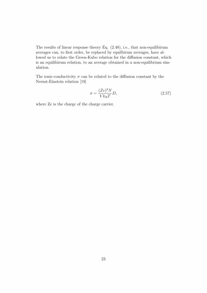
The results of linear response theory Eq. (2.48), i.e., that non-equilibirumaverages can, to first order, be replaced by equilbirum averages, have al-lowed us to relate the Green-Kubo relation for the diffusion constant, whichis an equilibirum relation, to an average obtained in a non-equilibrium sim-ulation.

The ionic-conductivity σ can be related to the diffusion constant by theNernst-Einstein relation [19]

σ =(Ze)2N

V kBTD, (2.57)

where Ze is the charge of the charge carrier.

23

Chapter 3

The Vienna ab-initiosimulation package

The code used for all simulations in this work is the Vienna ab-initio simu-lation package (VASP) [20, 21, 22, 23]. VASP uses DFT (and related meth-ods) to perform total energy calculations and BOMD. The KS orbitals areexpanded in a plane wave basis set, and interactions between the core- andvalence states are described via ultrasoft pseudopotentials or the PAWmethod (section 2.4). All calculations in VASP employs periodic bound-ary conditions. The classical EOM for the ionic-cores are integrated usinga velocity-Verlet scheme (section 2.5.2).

Normally, VASP requires 4 input files:

INCARThis is the main input file, which contains parameters specifying thecalculation procedure. These parameters can be divided into threesubgroups:- Parameters for electronic calculations: required accuracy,plane wave energy cutoff, electronic relaxation algorithm etc.- Parameters for ionic motion: MD-ensemble, initial temperature,timestep, etc.- Technical parameters: what output to write, how the calculationshould be parallelized over electron bands, k-points and plane wavecoefficients, etc.

POSCAR

24

The POSCAR file defines the supercell by specifying its lattice vec-tors and the position of the atoms. One may also chose to specify theinitial velocities of the atoms.

POTCARThis file contains the pseudo- or PAW potential. It essentially con-tains pre-calculations of the atomic core and core electrons, and alsospecifies the interaction between the valence and core electrons. Itcontains parameters such as, core radius, number of valence electronsand atomic masses. VASP comes with a library of POTCAR files,usually several different for the same elements differing in, for exam-ple, which electrons are treated as valence or as part of the core andthe core radius. This file also specifies which approximation to theXC-functional in DFT that is used.

KPOINTSThis file specifies the grid of k-points that are used to sample theBrillouin zone (see section 2.3).

25

Chapter 4

Model system: ceria

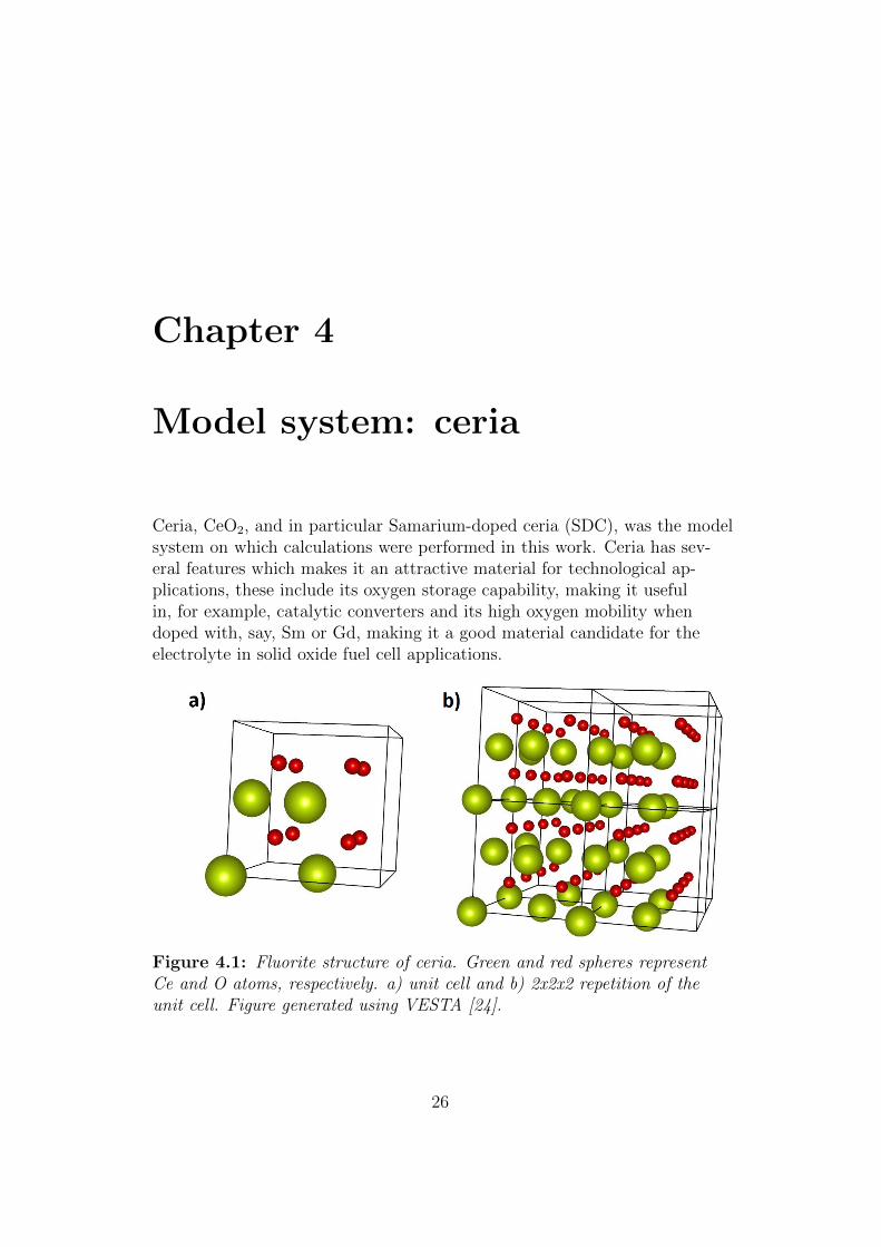
Ceria, CeO2, and in particular Samarium-doped ceria (SDC), was the modelsystem on which calculations were performed in this work. Ceria has sev-eral features which makes it an attractive material for technological ap-plications, these include its oxygen storage capability, making it usefulin, for example, catalytic converters and its high oxygen mobility whendoped with, say, Sm or Gd, making it a good material candidate for theelectrolyte in solid oxide fuel cell applications.

Figure 4.1: Fluorite structure of ceria. Green and red spheres representCe and O atoms, respectively. a) unit cell and b) 2x2x2 repetition of theunit cell. Figure generated using VESTA [24].

26

4.1 Structure

Ceria crystallises in the fluorite structure which can be viewed as the in-terpenetration of a simple cubic (sc) and a face centered cubic (fcc) lat-tice. The cerium atoms occupy the fcc lattice positions while the oxygenatoms occupy the positions of the sc lattice. Fig. 4.1 shows a unit cell anda 2x2x2 repetition of the unit cell, in which the green Ce atoms in the fcclattice and the red O atoms in the sc lattices can be clearly distinguished.

4.2 Doping and Ionic Conductivity

Normally, each Ce atom donates 4 electrons to the lattice which localises attwo different oxygen atoms yielding Ce4+ and O2−-ions.

Oxygen vacancies may form in perfect ceria, in which case the two left-overelectrons are likely to instead localise on close-by Ce4+, forming Ce3+-ions,or on impurity elements [25]. When ceria is doped with atoms of valence3+, such as Sm, oxygen vacancies are likely to form. More specifically, tokeep charge neutrality one oxygen vacancy needs to form for every pair ofSm dopants, thus in all calculations in this work one oxygen atom is re-moved for every two Sm atoms that are introduced into the simulation cell.

The introduction of vacancies into the oxygen lattice increases the mobilityof the O-ions leading to higher ionic conductivity. Since the concentrationof oxygen vacancies increases with Sm concentration, the ionic conductivityincreases with concentration up to a certain point where the effect of order-ing among vacancies and the fact that oxygen vacancies are less mobile inclose proximity to Sm3+ ions makes the ionic conductivity drop. In SDCthis optimal dopant concentration is around 15-20 % [26].

The diffusion of oxygen in ceria and doped ceria is expected to occur pri-marily by a vacancy hopping mechanism where an oxygen atom moves toone of its nearest neighbors (NN) in the sc sub-lattice.

27

4.3 Modeling ceria using DFT.

Many DFT studies have been performed on pure and doped ceria. The de-scription of the 4f electrons in Ce or Sm is known to be rather poor withinthe standard approximations to DFT. The LDA and GGA tend to givemuch too delocalised solutions.

This may not be a large issue if one expects there to form only Ce4+-ions,in which case all Ce atoms ”give away” its single 4f electron. For Ce3+ andSm3+, however, the issue needs to be addressed. This can be achieved byusing modifications to DFT such as LDA + U [27] or hybrid functionals[28, 29]. A simpler approach, which is the one used in the calculations inthis work, is to use a psuedo- or PAW-potential that treats the 4f electronsof Sm or Ce as part of the frozen core (see section 2.4).

28

Chapter 5

Methodological development

5.1 Implementing the color diffusion algorithm

Several complications arises when trying to calculate the diffusion constantfrom Eq. (2.56) in an actual computer simulation. In the following sectionsthe details in going from the theoretical results of section 2.5 to the im-plementation of a method to describe the diffusion process in our modelsystem, Sm doped ceria, will be presented.

5.1.1 Controlling the temperature

If one keeps applying the field this will continuously heat up to the sys-tem and no steady state will actually be reached1; the t → ∞ limit inEq. (2.56) will not exist unless one first takes the Fe → 0 limit, whichwe cannot do in the actual calculations, where we essentially want to takethe limits in the opposite order. This is solved by applying a thermostat(section 2.5.2) which continuously removes the energy added to the systemfrom the external field. One can show that the expression for the diffusionconstant is essentially the same for thermostated linear response [7].

One subtle issue here is that if the thermostat is applied to keep the in-

1A steady state here reefers to the situation where the color flux is unchanged withtime i.e., (d/dt) 〈J〉 = 0.

29

stantaneous temperature

Tinst. =2

3NkB

N∑i=1

p2i

2mi

(5.1)

constant then one may end up in a situation where the external field andthe thermostat just counteracts each other. The external field acceleratesthe atoms in a certain direction, which will lead to an increase of the tem-perature which is in turn counteracted by the thermostat, possibly leadingto a net acceleration that is lower than the desired one. In the original im-plementation by Evans et al. [3] this problem was addressed through cor-recting the temperature by only scaling the velocity components perpendic-ular to the field direction. Later [7, 30] this issues was instead resolved bydefining the instantaneous temperature w.r.t. the average velocity of theparticles, i.e.,

Tinst.avg. =2

3NkB

N∑i=1

(pi − cipciavg.)2

2mi

, (5.2)

where pciavg. is the average momentum of all atoms with color charge ci.

The next thing to consider is the introduction of several different atomicspecies into the system. If we take our SDC model system as an exam-ple, there are 3 different species of which we consider only the O atomsto be diffusive, i.e. we assume that the Ce and Sm atoms will only oscil-late around their equilibrium positions. We are therefor only interested inapplying the external field to the diffusing O atoms. One approach couldthen be to apply a thermostat controlling Tinst.avg. to the O atoms whileanother thermostat, controlling instead Tinst., would be used for the Ce/Smatoms.

A more straightforward approach, which is the one primarily used in thiswork, is to only control the temperature of the Ce/Sm subsystem. In thisway the temperature of the O subsystem is not explicitly controlled butis not allowed to continuously increase since the heat exchange with theCe/Sm atoms will prevent this from happening. This implies, of course,that the total temperature of the system cannot be explicitly controlledduring a simulation, but one can still keep the instantaneous temperaturewithin an interval. The advantages of this approach, other than its simplic-ity, is that we do not have to worry about the explicit effects the thermo-stat may have on the details of the dynamics of the diffusing atoms. It isinstructive at this points to formulate the equations of motion under which

30

our system of SDC evolves,

ri =pimi

, (5.3a)

pOi = FDFTi + ciFe, (5.3b)

pCe,Smi = FDFTi + ciFe + Fconstr. − αpCe,Smi , (5.3c)

where ci, ri and pi is the color charge, position and momentum of atom i,respectively, FDFT

i is the force on atom i obtained from the DFT calcula-tions and the last two terms in the last equation symbolically representsthe thermostat. Details of the thermostat are presented in section 5.2.

5.1.2 Choosing the Color Charge Distribution and theExternal Field Direction

Originally, the color diffusion algorithm was applied to the study of self dif-fusion in liquids. In this case the atoms are randomly given a color chargeci = ±1, such that

∑Ni=1 ci = 0 and self diffusion is simulated by the mixing

of the atoms with ci = ±1. A key difference between the diffusion processin a liquid and a solid is that in a solid it occurs via one or several specificmechanisms, while diffusion in a liquid is a disordered process. We will as-sume (and this needs to be validated after the calculations) that the exter-nal field is small enough that it does not change the mechanism by whichthe diffusion happens, but only ’speeds it up’. However, if one is not care-ful with how the color charges are distributed, it is possible to end up witha distribution that prevents the diffusion process from happening by thecorrect mechanism.

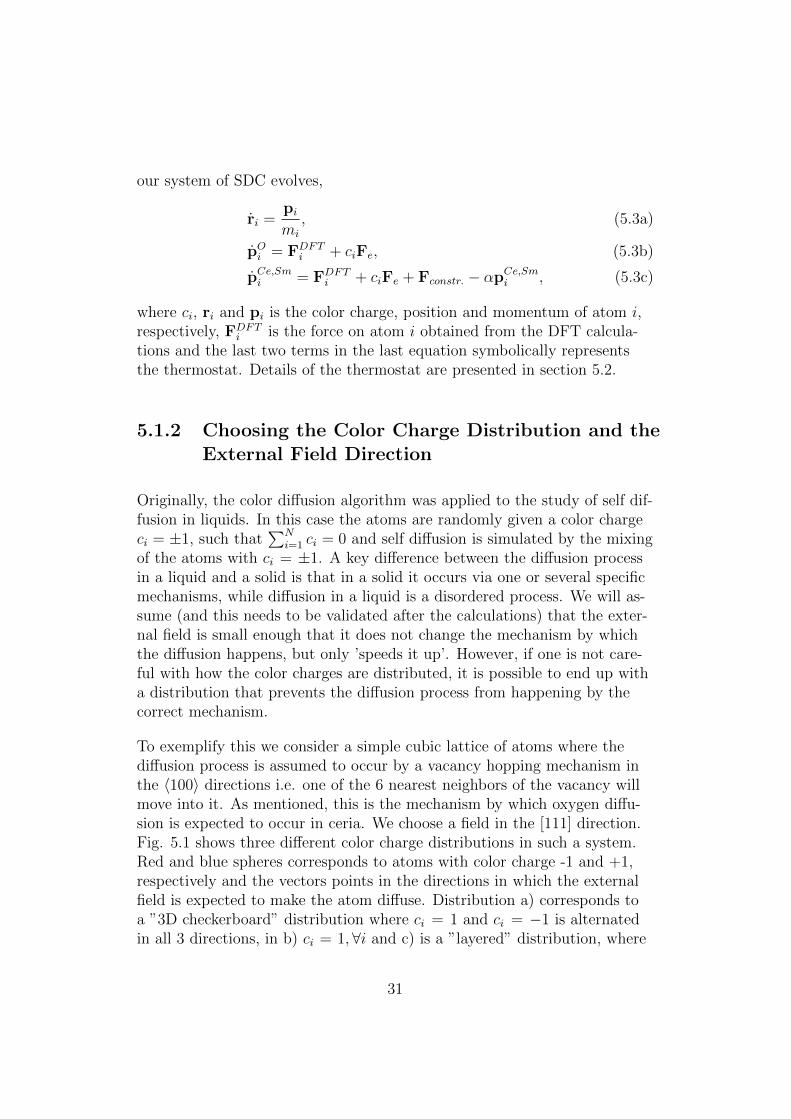
To exemplify this we consider a simple cubic lattice of atoms where thediffusion process is assumed to occur by a vacancy hopping mechanism inthe 〈100〉 directions i.e. one of the 6 nearest neighbors of the vacancy willmove into it. As mentioned, this is the mechanism by which oxygen diffu-sion is expected to occur in ceria. We choose a field in the [111] direction.Fig. 5.1 shows three different color charge distributions in such a system.Red and blue spheres corresponds to atoms with color charge -1 and +1,respectively and the vectors points in the directions in which the externalfield is expected to make the atom diffuse. Distribution a) corresponds toa ”3D checkerboard” distribution where ci = 1 and ci = −1 is alternatedin all 3 directions, in b) ci = 1, ∀i and c) is a ”layered” distribution, where

31

alternating (001) planes contains only +1 or -1 color charges. In all 3 casesa vacancy can be seen in the bottom near left corner.

Figure 5.1: Three possible initial color charge distributions: a) ”checker-board”, b) ”all plus” and c) ”layered”, see text for details. Red and bluespheres corresponds to -1 and +1 color charge, respectively.

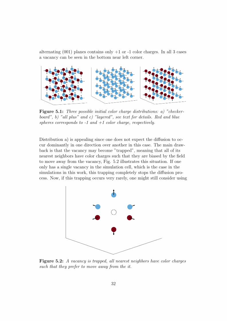
Distribution a) is appealing since one does not expect the diffusion to oc-cur dominantly in one direction over another in this case. The main draw-back is that the vacancy may become ”trapped”, meaning that all of itsnearest neighbors have color charges such that they are biased by the fieldto move away from the vacancy, Fig. 5.2 illustrates this situation. If oneonly has a single vacancy in the simulation cell, which is the case in thesimulations in this work, this trapping completely stops the diffusion pro-cess. Now, if this trapping occurs very rarely, one might still consider using

Figure 5.2: A vacancy is trapped, all nearest neighbors have color chargessuch that they prefer to move away from the it.

32

this distribution. To investigate the likelihood of the trapping a single va-cancy was moved in a 64 site simple cubic lattice into a nearest neighborwith the appropriate color charge until it was trapped. This procedure wasrepeated 10 000 times and a histogram of the number of vacancy jumpsuntil trapping occurred is shown in Fig. 5.3 along with the correspondingprobability distribution function (PDF).

During a long simulation we may expect to get on the order of 50 vacancyjumps, integrating the PDF in Fig. 5.3 from 0 to 50 gives a probability ofaround 16% that we encounter trapping during these 50 jumps, which isconsidered too high to be usable.

Figure 5.3: Histogram over number of jumps until the vacancy getstrapped. The vacancy is randomly moved into one of it nearest neighborwith color charge such that it prefers to move into the vacancy, as ex-plained in the text. The color charges are given by the checkerboard dis-tribution of Fig. 5.1 a). The corresponding PDF is shown to the right.

Using distribution c) would most certainly make the occurrence of thiskind of trapping very unlikely. However, in this case we introduce a pre-ferred direction of diffusion. It is easy to see that diffusion will occur mainlyin the 110 planes. One could consider using 3 different layered distribu-tions, with alternating planes of +1 and -1 color charge in the [100],[010]and [001] directions, and then averaging the calculated quantities overthe 3 distributions. This distribution may also be interesting to use if oneknows that the diffusion occurs mostly in one or several specific directions[2].

In both cases a) and c) the system is close to being color charge neutral,

33

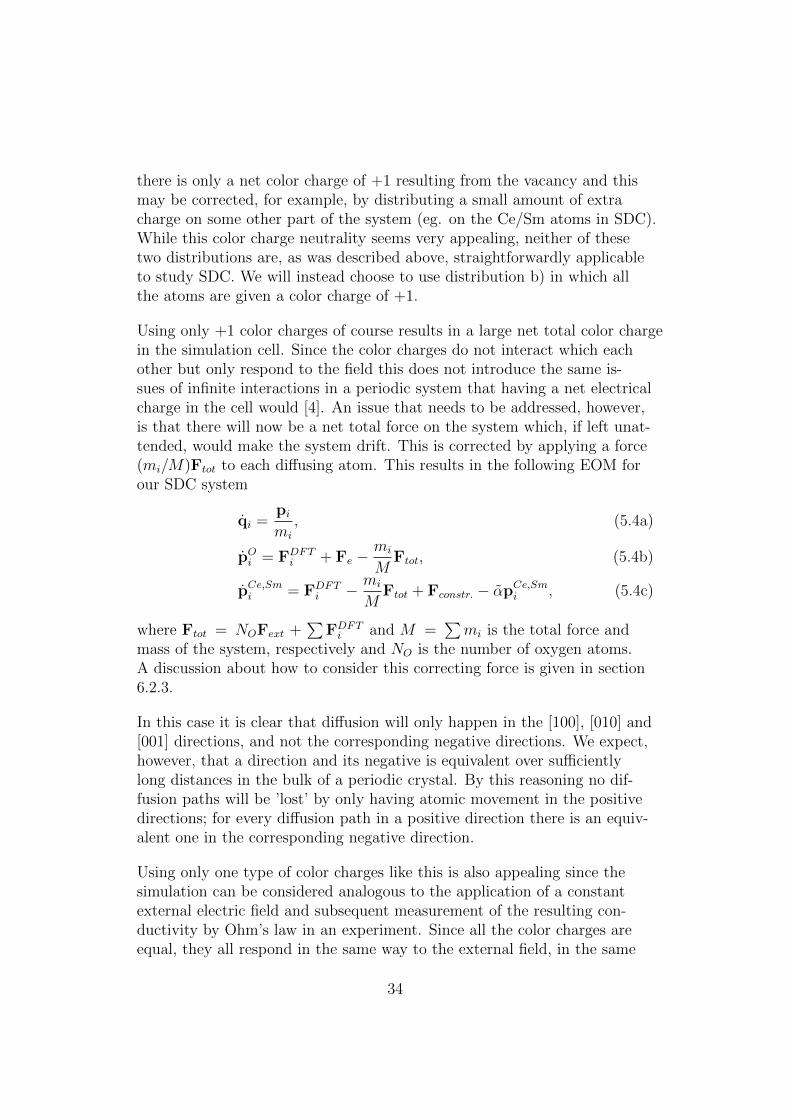
there is only a net color charge of +1 resulting from the vacancy and thismay be corrected, for example, by distributing a small amount of extracharge on some other part of the system (eg. on the Ce/Sm atoms in SDC).While this color charge neutrality seems very appealing, neither of thesetwo distributions are, as was described above, straightforwardly applicableto study SDC. We will instead choose to use distribution b) in which allthe atoms are given a color charge of +1.

Using only +1 color charges of course results in a large net total color chargein the simulation cell. Since the color charges do not interact which eachother but only respond to the field this does not introduce the same is-sues of infinite interactions in a periodic system that having a net electricalcharge in the cell would [4]. An issue that needs to be addressed, however,is that there will now be a net total force on the system which, if left unat-tended, would make the system drift. This is corrected by applying a force(mi/M)Ftot to each diffusing atom. This results in the following EOM forour SDC system

qi =pimi

, (5.4a)

pOi = FDFTi + Fe −

mi

MFtot, (5.4b)

pCe,Smi = FDFTi − mi

MFtot + Fconstr. − αpCe,Smi , (5.4c)

where Ftot = NOFext +∑

FDFTi and M =

∑mi is the total force and

mass of the system, respectively and NO is the number of oxygen atoms.A discussion about how to consider this correcting force is given in section6.2.3.

In this case it is clear that diffusion will only happen in the [100], [010] and[001] directions, and not the corresponding negative directions. We expect,however, that a direction and its negative is equivalent over sufficientlylong distances in the bulk of a periodic crystal. By this reasoning no dif-fusion paths will be ’lost’ by only having atomic movement in the positivedirections; for every diffusion path in a positive direction there is an equiv-alent one in the corresponding negative direction.

Using only one type of color charges like this is also appealing since thesimulation can be considered analogous to the application of a constantexternal electric field and subsequent measurement of the resulting con-ductivity by Ohm’s law in an experiment. Since all the color charges areequal, they all respond in the same way to the external field, in the same

34

way that ions of the same charge will respond the same to a (weak) exter-nal electric field. The [111] field direction also merges nicely into this anal-ogy. In a conductivity experiment the sample will contain grains that willhave different crystal directions aligned with the field, the [111] field direc-tion in the perfect bulk crystal is the one that most closely corresponds toan average over different directions in different grains of the experimentalsample.

5.2 Technical details in the implementation

While the method is formally complete with the EOM (5.4) and the ex-pression for the diffusion constant Eq. (2.56), there are several technicaldetails in the implementation that need to be addressed. In the followingwe assume that the system we are modeling is SDC.

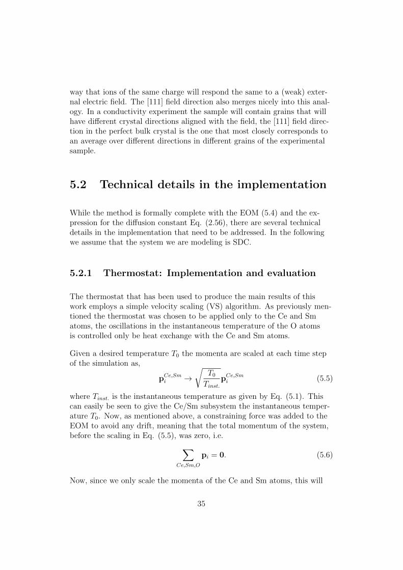
5.2.1 Thermostat: Implementation and evaluation

The thermostat that has been used to produce the main results of thiswork employs a simple velocity scaling (VS) algorithm. As previously men-tioned the thermostat was chosen to be applied only to the Ce and Smatoms, the oscillations in the instantaneous temperature of the O atomsis controlled only be heat exchange with the Ce and Sm atoms.

Given a desired temperature T0 the momenta are scaled at each time stepof the simulation as,

pCe,Smi →√

T0Tinst.

pCe,Smi (5.5)

where Tinst. is the instantaneous temperature as given by Eq. (5.1). Thiscan easily be seen to give the Ce/Sm subsystem the instantaneous temper-ature T0. Now, as mentioned above, a constraining force was added to theEOM to avoid any drift, meaning that the total momentum of the system,before the scaling in Eq. (5.5), was zero, i.e.∑

Ce,Sm,O

pi = 0. (5.6)

Now, since we only scale the momenta of the Ce and Sm atoms, this will

35

generally result in a nonzero total momentum2. To avoid the drift the aver-age momenta of all atoms is removed from each Ce and Sm atom accordingto

pCe,Smi → pCe,Smi − 1

NCe,Sm

∑O,Ce,Sm

pi, (5.7)

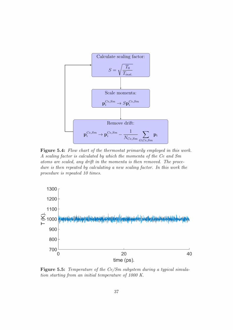
where the right arrow signifies a replacement. This operation will, as a con-sequence of altering the momenta, change the temperature of the Ce/Smsubsystem. We expect, however, that if we apply the scaling in Eq. (5.5)with the new momenta, obtained through Eq. (5.7), each subsequent appli-cation of Eq. (5.7) will alter the temperature less and less. One can thenperform the velocity scaling and drift correction over and over, either un-til the temperature change by performing the drift correction is lower thansome tolerance, or just a fix number of times that keeps the temperaturesufficiently constant. For the calculations in this work performing this cy-cle 10 times was seen to be sufficient. Figs. 5.4 and 5.5 show a schematicflow chart of the implementation of the thermostat and the resulting tem-perature of the Ce/Sm subsystem during a typical simulation at 1000 K,respectively.

A discussion about how this thermostat affects the temperature of the oxy-gen subsystem, as well as what should be considered to be the ”real” tem-perature of the system is given in section 6.2.4.

5.2.2 Calculating the steady state color flux

Calculation of the diffusion constant Eq. (2.56) requires the evaluation ofthe steady state color flux (SSF) which in the case of color charges ci = 1for all oxygen atoms is given by,

〈J〉S =

⟨1

V

∑O

vi

⟩S

. (5.8)

Here, vi is the velocity component in the direction of the external field andV is the volume of the simulation cell. The most straightforward way ofevaluating 〈J〉 is by simply taking the time average at each simulation

2This is opposed to the case where the momenta of all the atoms are scaled:∑pi = 0 =⇒ S

∑pi = 0.

36

Calculate scaling factor:

S =

√T0Tinst.

Scale momenta:

pCe,Smi → SpCe,Smi

Remove drift:

pCe,Smi → pCe,Smi − 1

NCe,Sm

∑O,Ce,Sm

pi

Figure 5.4: Flow chart of the thermostat primarily employed in this work.A scaling factor is calculated by which the momenta of the Ce and Smatoms are scaled, any drift in the momenta is then removed. The proce-dure is then repeated by calculating a new scaling factor. In this work theprocedure is repeated 10 times.

Figure 5.5: Temperature of the Ce/Sm subystem during a typical simula-tion starting from an initial temperature of 1000 K.

37

step, k, and observing the convergence, i.e.,

〈J〉 (k) =1

k∆t

k∑t=k0

(1

V

∑O

vi(t)

), (5.9)

where ∆t is the timestep of the simulation. When the external field is firstapplied to the system it will have a transient period where the response islarge before a steady state is reached. Choosing this period to be 500 MDsteps, i.e. letting k0 = 500 in the equation above was seen to be sufficient.Fig. 5.6 shows the response J = (1/V )

∑O vi and 〈J〉 (k) during a typical

run. Note the appearance of convergence of 〈J〉 (k).

Figure 5.6: J = (1/V )∑

0 vi and the time average 〈J〉 during a typicalsimulation. The dotted line signifies the convergence of 〈J〉.

As was mentioned above we do not consider the external field to qualita-tively alter the dynamics of our system, but to only accelerate the diffusionprocess. This means that if there are no oxygen jumps, we expect all atomsto oscillate around their equilibrium lattice position. Hence, in the absence

38

of jumps, we should have 〈J〉 = 0, and the only reason that we see a con-vergence of 〈J〉 (k) towards a positive value in Fig. 5.6 is because of thediffusive jumps of the oxygen atoms in the direction of the field. By thisreasoning we should be able to calculate the SSF by only monitoring thepositions of the oxygen atoms. More precisely, integrating the expressionfor J yields, ∫ t

0

J(τ)dτ =1

V

∑O

(xi(t)− xi(0)) . (5.10)

Now, a true steady state is characterised by (d/dt) 〈J〉 = 0 which togetherwith Eq. (5.10) gives,

〈J〉 =1

V

⟨d

dt

(∑O

(xi(t)− xi(0))

)⟩=

⟨d

dt(C1t+ C2)

⟩= C1, (5.11)

where C1 and C2 are constants. Thus, a way to calculate the SSF is to findthe slope of the linear fit to the right hand side in Eq. (5.10). One shouldalso note that the goodness of the linear fit in Eq. (5.11) gives a directmeasure of how close the system is to a true steady state.

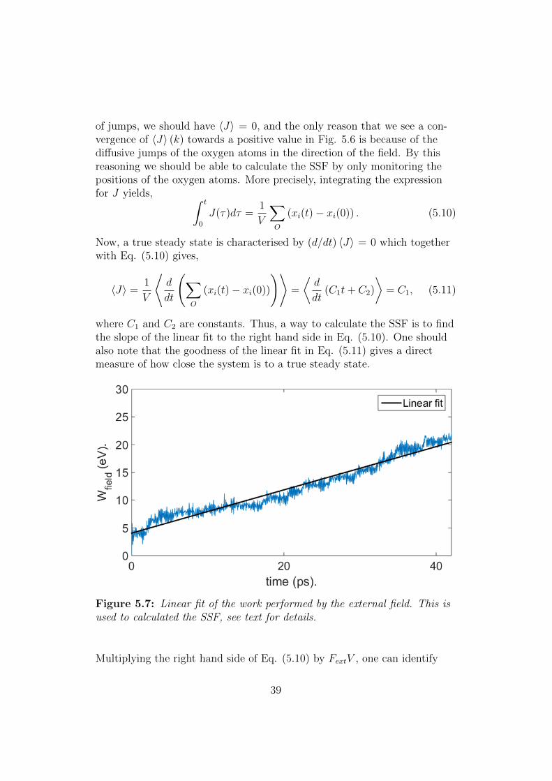
Figure 5.7: Linear fit of the work performed by the external field. This isused to calculated the SSF, see text for details.

Multiplying the right hand side of Eq. (5.10) by FextV , one can identify

39

the work performed on the system by the external field,

Wfield = Fext∑O

(xi(t)− xi(0)) . (5.12)

Fig. 5.7 shows Wfield and the corresponding linear fit which is used to cal-culated the SSF during a typical simulation.

5.2.3 Choosing the strength of the external field: Thelinear regime

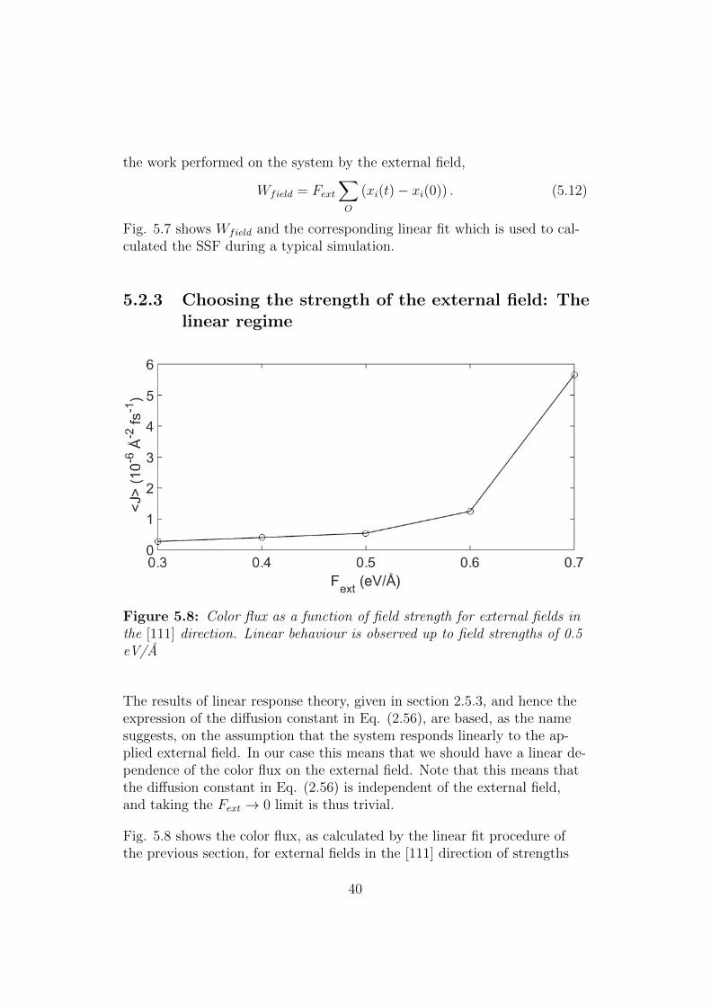
Figure 5.8: Color flux as a function of field strength for external fields inthe [111] direction. Linear behaviour is observed up to field strengths of 0.5eV/A

The results of linear response theory, given in section 2.5.3, and hence theexpression of the diffusion constant in Eq. (2.56), are based, as the namesuggests, on the assumption that the system responds linearly to the ap-plied external field. In our case this means that we should have a linear de-pendence of the color flux on the external field. Note that this means thatthe diffusion constant in Eq. (2.56) is independent of the external field,and taking the Fext → 0 limit is thus trivial.

Fig. 5.8 shows the color flux, as calculated by the linear fit procedure ofthe previous section, for external fields in the [111] direction of strengths

40

0.3, 0.4, 0.5, 0.6 and 0.7 eV/A. We see that the response appears largelylinear up to and including fields strengths of 0.5 eV/A after which non-linear behaviour is observed. An external field of strength 0.5 eV/A in the[111] direction was thus used for all simulations.

5.2.4 Identifying the vacancies

In the above we have taken the viewpoint that the diffusion mechanism isone in which O atoms jumps into a vacancy located at any of its 6 nearestneighbor lattice sites. One can, however, equally well consider the diffusionprocess as happening through the movement of the vacancy, which thenwill move in the opposite direction of the O atom. A lot of insight into thediffusion process can then be gained by analysing the position of the va-cancy during a simulation.

We will consider the case of identifying oxygen vacancies in SDC. Spheresof radii aO/2, where aO is the lattice constant of the oxygen sub-lattice,can then be placed centered at each lattice position. Now, since these spheresdo not cover the whole simulation cell and since the thermal oscillationscan be rather large at the temperatures in use a lattice position cannotsimply be identified as being vacant if its surrounding sphere does not con-tain an oxygen atom at a single step in the MD simulation. Instead a lat-tice position is considered to contain a vacancy at a time t if the spherecentered at this position is empty at t − 5∆t, t and t + 5∆t. It turns outthat this may not be a sufficient condition to identify the vacancy in all sit-uations either, for example, problems may occur when two oxygen atomssimultaneously try to move into a vacancy. It is, however, rather easy tomanually identify and remove cases of ”false” vacancies in the post process-ing.

Note that the spheres around lattice positions at the edges of the simula-tion cell has to be periodically repeated at the opposite side of the simula-tion cell when the vacancies are being identified.

41

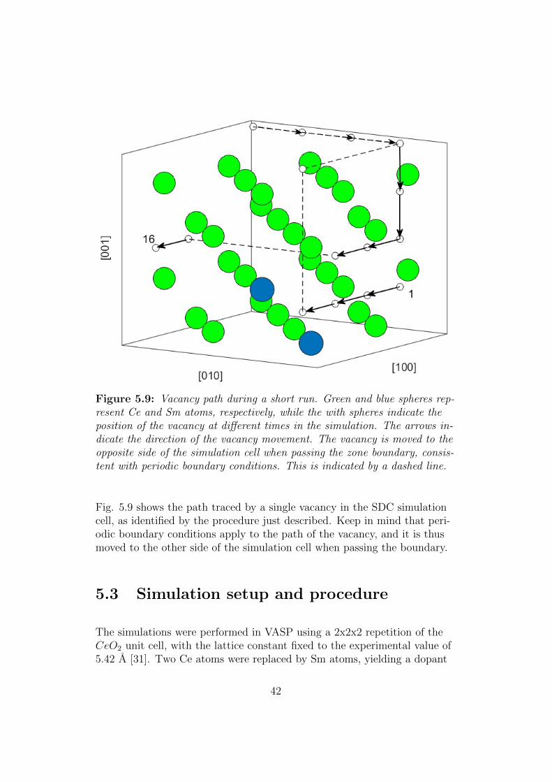
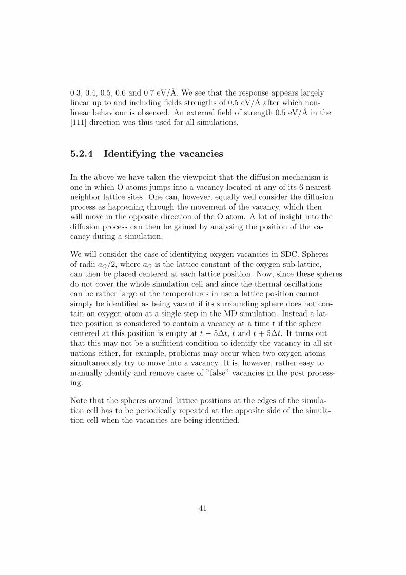
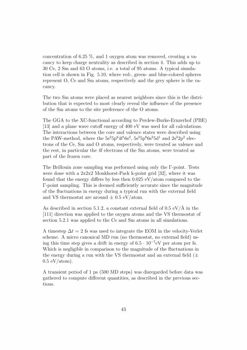
Figure 5.9: Vacancy path during a short run. Green and blue spheres rep-resent Ce and Sm atoms, respectively, while the with spheres indicate theposition of the vacancy at different times in the simulation. The arrows in-dicate the direction of the vacancy movement. The vacancy is moved to theopposite side of the simulation cell when passing the zone boundary, consis-tent with periodic boundary conditions. This is indicated by a dashed line.

Fig. 5.9 shows the path traced by a single vacancy in the SDC simulationcell, as identified by the procedure just described. Keep in mind that peri-odic boundary conditions apply to the path of the vacancy, and it is thusmoved to the other side of the simulation cell when passing the boundary.

5.3 Simulation setup and procedure

The simulations were performed in VASP using a 2x2x2 repetition of theCeO2 unit cell, with the lattice constant fixed to the experimental value of5.42 A [31]. Two Ce atoms were replaced by Sm atoms, yielding a dopant

42

concentration of 6.25 %, and 1 oxygen atom was removed, creating a va-cancy to keep charge neutrality as described in section 4. This adds up to30 Ce, 2 Sm and 63 O atoms, i.e. a total of 95 atoms. A typical simula-tion cell is shown in Fig. 5.10, where red-, green- and blue-colored spheresrepresent O, Ce and Sm atoms, respectively and the grey sphere is the va-cancy.

The two Sm atoms were placed as nearest neighbors since this is the distri-bution that is expected to most clearly reveal the influence of the presenceof the Sm atoms to the site preference of the O atoms.

The GGA to the XC-functional according to Perdew-Burke-Ernzerhof (PBE)[13] and a plane wave cutoff energy of 400 eV was used for all calculations.The interactions between the core and valence states were described usingthe PAW-method, where the 5s25p64f16s2, 5s25p66s25d1 and 2s22p2 elec-trons of the Ce, Sm and O atoms, respectively, were treated as valence andthe rest, in particular the 4f electrons of the Sm atoms, were treated aspart of the frozen core.

The Brillouin zone sampling was performed using only the Γ-point. Testswere done with a 2x2x2 Monkhorst-Pack k-point grid [32], where it wasfound that the energy differs by less then 0.025 eV/atom compared to theΓ-point sampling. This is deemed sufficiently accurate since the magnitudeof the fluctuations in energy during a typical run with the external fieldand VS thermostat are around ± 0.5 eV/atom.

As described in section 5.1.2, a constant external field of 0.5 eV/A in the[111] direction was applied to the oxygen atoms and the VS thermostat ofsection 5.2.1 was applied to the Ce and Sm atoms in all simulations.

A timestep ∆t = 2 fs was used to integrate the EOM in the velocity-Verletscheme. A micro canonical MD run (no thermostat, no external field) us-ing this time step gives a drift in energy of 6.5 · 10−7eV per atom per fs.Which is negligible in comparison to the magnitude of the fluctuations inthe energy during a run with the VS thermostat and an external field (±0.5 eV/atom).

A transient period of 1 ps (500 MD steps) was disregarded before data wasgathered to compute different quantities, as described in the previous sec-tions.

43

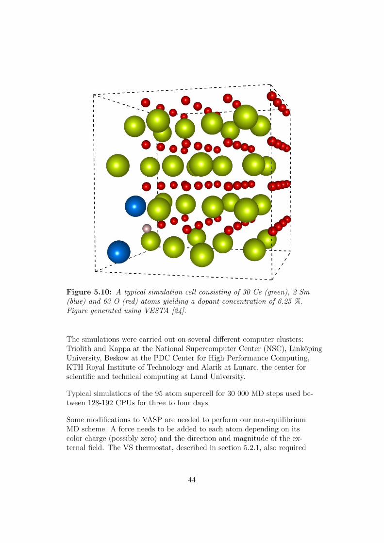
Figure 5.10: A typical simulation cell consisting of 30 Ce (green), 2 Sm(blue) and 63 O (red) atoms yielding a dopant concentration of 6.25 %.Figure generated using VESTA [24].

The simulations were carried out on several different computer clusters:Triolith and Kappa at the National Supercomputer Center (NSC), LinkopingUniversity, Beskow at the PDC Center for High Performance Computing,KTH Royal Institute of Technology and Alarik at Lunarc, the center forscientific and technical computing at Lund University.

Typical simulations of the 95 atom supercell for 30 000 MD steps used be-tween 128-192 CPUs for three to four days.

Some modifications to VASP are needed to perform our non-equilibriumMD scheme. A force needs to be added to each atom depending on itscolor charge (possibly zero) and the direction and magnitude of the ex-ternal field. The VS thermostat, described in section 5.2.1, also required

44

some additions to the VASP code3. To this end another input file was in-troduced:

infile.colorchargesThis file contains the external field vector, the color charge of eachatom and a flag for each atom specifying if its velocity should bescaled by the VS thermostat.

3Thanks are due to Dr. Olle Hellman and Johan Nilsson for writing and providingthis modified VASP-code at the start of the diploma work.

45

Chapter 6

Results and Discussion

6.1 Results

In this section results of simulations carried out with the method describedin the previous sections are presented. Good agreement with experimentalresults is found, both in the numerical values and temperature dependenceof the conductivity and in the details of the diffusion process.

6.1.1 Ionic conductivity

Simulations was caried out at initial temperatures of 800, 900, 1000, 1100and 1200 K, with parameters as described in section 5.3. Now, since thesimulation cell (Figure 5.10) contains two Sm dopants, different vacancypositions and paths will be non-equivalent depending on their positionin relation to the dopants, to make the vacancy visit the largest possiblenumber of lattice sites during the simulations the calculations were startedfrom several (2-4 as seen in Fig. 6.1) different initial vacancy positions.The resulting ionic conductivities are shown in Fig. 6.1. As expected fromthe considerations in section 5.2.1 the mean temperature of simulationsstarted at the same initial temperature differs slightly.

In Fig. 6.2 averages have been taken of both conductivities and mean tem-peratures for all initial vacancy positions at the same initial temperature.The conductivities (log-scale) are plotted versus inverse temperature. Ex-

46

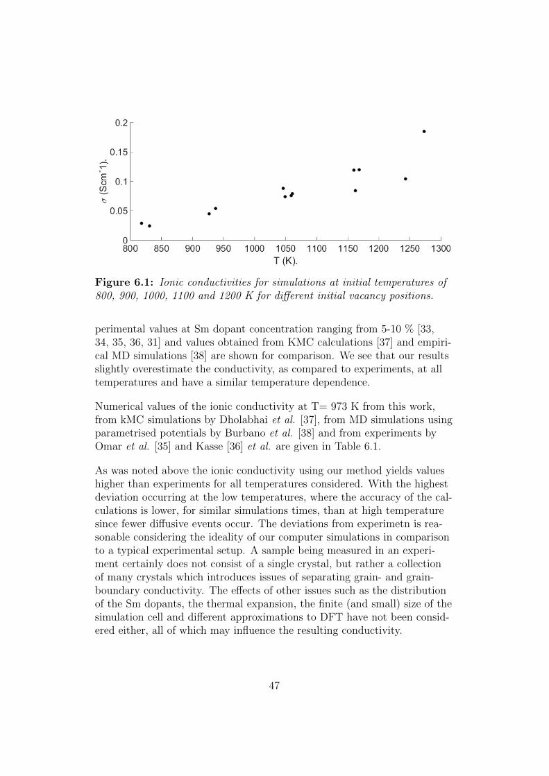
Figure 6.1: Ionic conductivities for simulations at initial temperatures of800, 900, 1000, 1100 and 1200 K for different initial vacancy positions.

perimental values at Sm dopant concentration ranging from 5-10 % [33,34, 35, 36, 31] and values obtained from KMC calculations [37] and empiri-cal MD simulations [38] are shown for comparison. We see that our resultsslightly overestimate the conductivity, as compared to experiments, at alltemperatures and have a similar temperature dependence.

Numerical values of the ionic conductivity at T= 973 K from this work,from kMC simulations by Dholabhai et al. [37], from MD simulations usingparametrised potentials by Burbano et al. [38] and from experiments byOmar et al. [35] and Kasse [36] et al. are given in Table 6.1.

As was noted above the ionic conductivity using our method yields valueshigher than experiments for all temperatures considered. With the highestdeviation occurring at the low temperatures, where the accuracy of the cal-culations is lower, for similar simulations times, than at high temperaturesince fewer diffusive events occur. The deviations from experimetn is rea-sonable considering the ideality of our computer simulations in comparisonto a typical experimental setup. A sample being measured in an experi-ment certainly does not consist of a single crystal, but rather a collectionof many crystals which introduces issues of separating grain- and grain-boundary conductivity. The effects of other issues such as the distributionof the Sm dopants, the thermal expansion, the finite (and small) size of thesimulation cell and different approximations to DFT have not been consid-ered either, all of which may influence the resulting conductivity.

47

Figure 6.2: Ionic conductivities from this work showed as a solid blackline. Experimental results [33, 34, 35, 36, 31] (dashed lines) and theoreticalresults (solid lines) [37, 38] are shown for comparison. Square, circle anddiamond markers corresponds to Sm dopant concentrations of 5%, 6.25%and 10%, respectively

Ionic conductivity, σ, at T = 973 K

MethodDopantconcentration (%)

σ (Scm−1) Source

NEMD 6.25 0.060 This workKMC 5 0.0033 Dholabhai et al. [37]

10 0.0052MD 5 0.013 Burbano et al. [38]

10 0.014Experiment 5 0.025 Omar et al. [35]

10 0.046 Kasse et al. [36]

Table 6.1: Ionic conductivities at T = 973 K obtained in this work andfrom classical MD [38], KMC [37] and experiments [35, 36]. The classicalMD and NEMD values are linear interpolations from the 2 closest tempera-tures at which the conductivities were calculated.

48

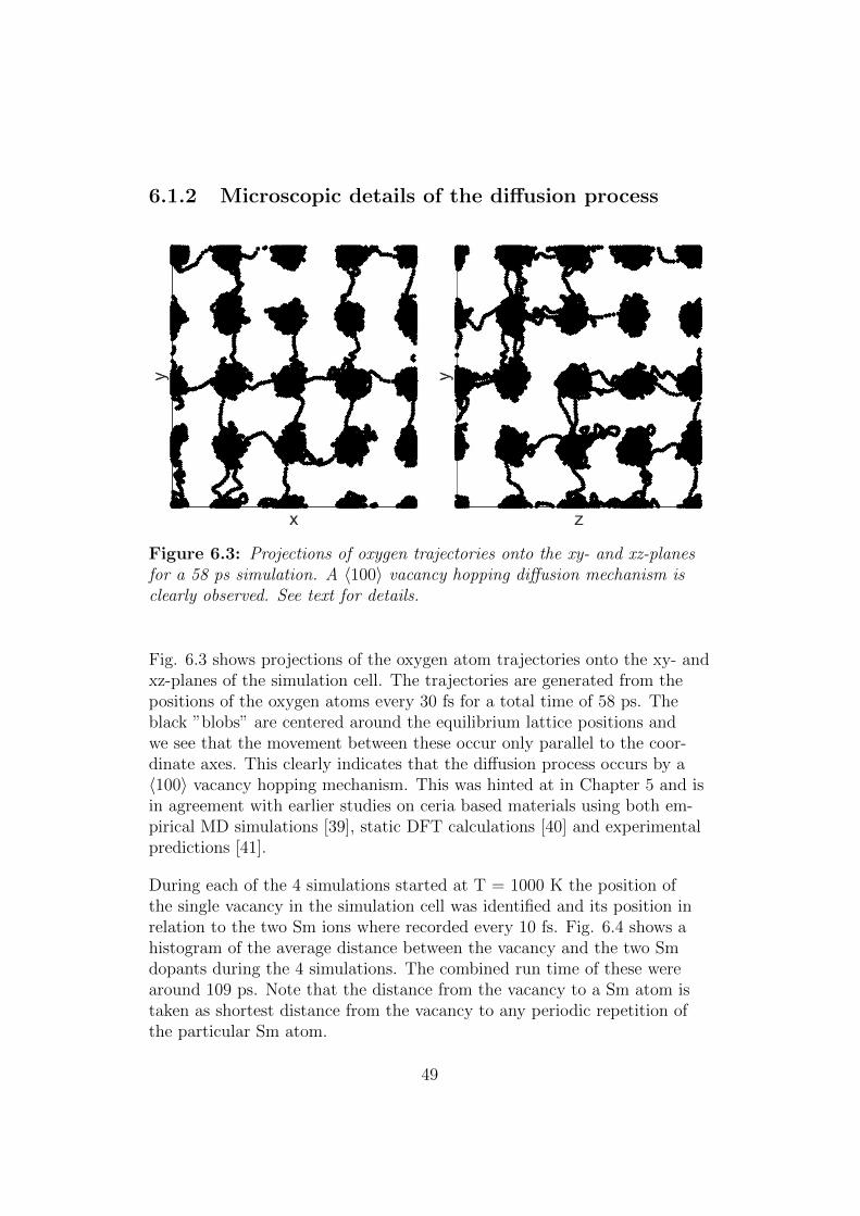
6.1.2 Microscopic details of the diffusion process

Figure 6.3: Projections of oxygen trajectories onto the xy- and xz-planesfor a 58 ps simulation. A 〈100〉 vacancy hopping diffusion mechanism isclearly observed. See text for details.

Fig. 6.3 shows projections of the oxygen atom trajectories onto the xy- andxz-planes of the simulation cell. The trajectories are generated from thepositions of the oxygen atoms every 30 fs for a total time of 58 ps. Theblack ”blobs” are centered around the equilibrium lattice positions andwe see that the movement between these occur only parallel to the coor-dinate axes. This clearly indicates that the diffusion process occurs by a〈100〉 vacancy hopping mechanism. This was hinted at in Chapter 5 and isin agreement with earlier studies on ceria based materials using both em-pirical MD simulations [39], static DFT calculations [40] and experimentalpredictions [41].

During each of the 4 simulations started at T = 1000 K the position ofthe single vacancy in the simulation cell was identified and its position inrelation to the two Sm ions where recorded every 10 fs. Fig. 6.4 shows ahistogram of the average distance between the vacancy and the two Smdopants during the 4 simulations. The combined run time of these werearound 109 ps. Note that the distance from the vacancy to a Sm atom istaken as shortest distance from the vacancy to any periodic repetition ofthe particular Sm atom.

49

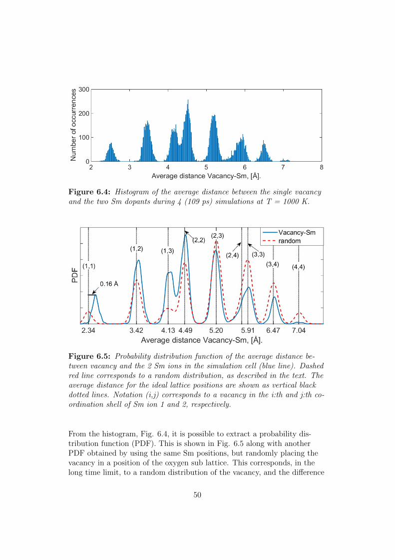
Figure 6.4: Histogram of the average distance between the single vacancyand the two Sm dopants during 4 (109 ps) simulations at T = 1000 K.

Figure 6.5: Probability distribution function of the average distance be-tween vacancy and the 2 Sm ions in the simulation cell (blue line). Dashedred line corresponds to a random distribution, as described in the text. Theaverage distance for the ideal lattice positions are shown as vertical blackdotted lines. Notation (i,j) corresponds to a vacancy in the i:th and j:th co-ordination shell of Sm ion 1 and 2, respectively.

From the histogram, Fig. 6.4, it is possible to extract a probability dis-tribution function (PDF). This is shown in Fig. 6.5 along with anotherPDF obtained by using the same Sm positions, but randomly placing thevacancy in a position of the oxygen sub lattice. This corresponds, in thelong time limit, to a random distribution of the vacancy, and the difference

50

between these two PDFs reveals the influence of the Sm dopants on thepreferred position of the oxygen vacancy. The average distances obtainedfrom the atoms sitting in their ideal lattice positions are indicated as dot-ted black vertical lines, where the notation (i,j) indicates that the vacancyis in the i:th and j:th coordination shell of the first and second Sm dopant,respectively.

Several interesting features can be observed. First we see that the oxygenvacancy clearly prefers to sit close to the Sm atoms. This is seen by ob-serving that the peaks corresponding to the 4 closest average distances, i.ethe (1,1), (1,2), (1,3) and (2,2) peaks, are higher than the correspondingpeaks of the random vacancy distribution, while the 5 remaining peaks,corresponding to the vacancy sitting further away from the vacancy, arelower. This is in agreement with previous static DFT studies [42, 43] whereit is shown that the vacancy positions close to the dopants corresponds tothe lowest energy configurations, and also that the oxygen migration bar-riers are higher for diffusion paths close to the dopants than for paths faraway from the them.

Secondly, there is a clear shift of the (1,1)-peak towards higher average dis-tance compared to the ideal value. This suggests that the dopant atomstend to shift their equilibrium positions away from the vacancy when inthe NN position. As indicated in the figure, the average shift is 0.16 A.This has been observed in several previous studies [44, 43] where, for ex-ample, Andersson et al. [43] finds that the equilibrium positions of the twodopants in the NN position shifts 0.13 - 0.19 A away from the vacancy de-pending on the type of dopant used.

6.2 Discussion

6.2.1 Temperature dependence of the linear regime

As can be seen in Fig. 6.1 the values of the conductivity have a much largerspread at the highest temperature point. This was seen as an indicationthat the linear regime may, in fact, be temperature dependent. A similartest of field strength versus flux as the one performed at 1000 K in sec-tion 5.2.3 was run at 1200 K. The results are shown in Fig. 6.6 where wecan see that a field strength of 0.5 eV/A in fact appears to be outside the

51

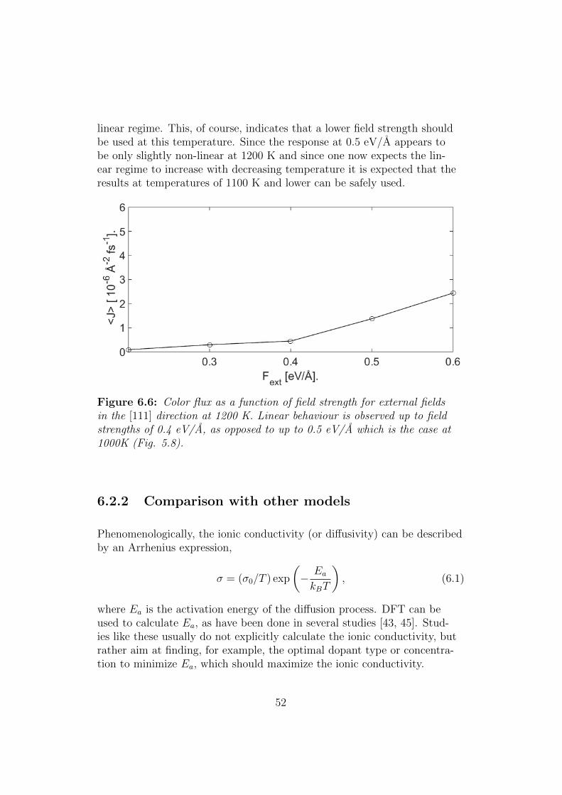
linear regime. This, of course, indicates that a lower field strength shouldbe used at this temperature. Since the response at 0.5 eV/A appears tobe only slightly non-linear at 1200 K and since one now expects the lin-ear regime to increase with decreasing temperature it is expected that theresults at temperatures of 1100 K and lower can be safely used.

Figure 6.6: Color flux as a function of field strength for external fieldsin the [111] direction at 1200 K. Linear behaviour is observed up to fieldstrengths of 0.4 eV/A, as opposed to up to 0.5 eV/A which is the case at1000K (Fig. 5.8).

6.2.2 Comparison with other models

Phenomenologically, the ionic conductivity (or diffusivity) can be describedby an Arrhenius expression,

σ = (σ0/T ) exp

(− EakBT

), (6.1)

where Ea is the activation energy of the diffusion process. DFT can beused to calculate Ea, as have been done in several studies [43, 45]. Stud-ies like these usually do not explicitly calculate the ionic conductivity, butrather aim at finding, for example, the optimal dopant type or concentra-tion to minimize Ea, which should maximize the ionic conductivity.

52

Another possibility is to use the calculated activation energy as an inputinto a KMC scheme, where a system is propagated between between dif-ferent states separated by a vacancy hopping event. The transition ratesare then given by an Arrhenius type expression. From this it is possible tocalculate the diffusion constant using the Einstein relation1,

D = limt→∞

1

6NOt

NO∑i=1

(ri(t)− ri(0))2 , (6.2)

where 1NO

∑NO

i=1 (ri(t)− ri(0))2 is the mean squared displacement (MSD)of the oxygen atoms. This was the method used by Dholabhai et al. [37].Their resulting ionic conductivities are given in Fig. 6.2. We see that theirresults are lower than experiments with the best agreement occurring atlower temperature.

It is natural that the best results from the KMC simulations occurs at lowtemperature since the barriers of diffusion are calculated at T = 0 K, andtemperature effects are only taking into consideration when propagatingthe system between states. The barriers are, however, very much dynam-ical in reality. Since the atoms are thermally oscillating at finite tempera-ture the oxygen migration barrier is certainly expected to change depend-ing on the positions of the neighboring cations at the time of diffusion.

If one is able to simulate for long enough time Eq. (6.2) can be used tocalculate the diffusion constant in a MD simulation as well, these simula-tion times can, however, only be achieved using parametrised expression forthe interaction potentials. Such calculations were performed by Burbanoet al. [38], who simulated a 2600 atom SDC system for times on the orderof nanoseconds. These results are shown in Fig. 6.2 where we see that thismethod also underestimates the ionic conductivity, but is in better agree-ment with experiment than the KMC results discussed above, and withdeviations from experimental values of the same order as the results pre-sented in this work.

6.2.3 The correctional force

As mentioned in section 5.1.2 a correctional force was added to the systemto avoid the drift originating from the net color charge in the system, re-

1This is equivalent to the Green-Kubo relation for the diffusion constant Eq. 2.50

53

sulting in the EOM (5.4), which are reproduced here:

qi =pimi

, (6.3a)

pOi = FDFTi + Fe −

mi

MFtot, (6.3b)

pCe,Smi = FDFTi − mi

MFtot + Fconstr. − αpCe,Smi , (6.3c)

An interesting question is now how one should consider this correctionalforce, mi∑

mjFtot. There are essentially two possible options:

(I) It should be treated as part of the external field, giving an ”effectiveexternal field”

Feffext = Fext −

mO∑mj

Ftot. (6.4)

(II) It should not be treated as a part of the external force but only as fix-ing the reference frame.

If one would go with option (I) this will result in a correction to the ob-tained conductivities. The total force on the system is the sum of the DFTcalculated forces and the sum of the external force we apply to each oxygenatoms,

Ftot = NOFext +∑

O,Ce,Sm

FDFTi . (6.5)

The sum of the DFT calculated forces should formally be zero, although anonzero value is to be expected because of numerical inaccuracies, and wewill consider it to vanish. This gives an effective external force,

Feffext = Fext −

NOmO∑mj

Fext

=

(1− NOmO

NOmO +NCemCe +NSmmSm

)Fext

= CFext.

(6.6)

where NO, NCe and NSm are the number of O, Ce and Sm atoms in thesystem, respectively and C ≈ 0.8171. Which means that all results shouldbe multiplied by a factor 1/C. It may be interesting to note that this takesthe results further away from the experimental values.

The simple argument for option (I) is the following: if there were no exter-nal force this would imply that the correctional force would be zero as well,

54

i.e. the external field is the cause of the correctional force and they shouldthus both be combined to give an effective external force.

However, one should theoretically be able to simulate the diffusion in anyreference frame, moving or not, it just consists of the movement of the Oatoms relative to the non diffusive Ce/Sm atoms. Although this would bevery inconvenient from a computational point of view, it would suggestthat the correctional force is just there to fix the reference frame implyingthere would be no need to consider an effective external field, and option(II) would be valid.

6.2.4 Temperature considerations

Figure 6.7: Temperature of the O and Ce/Sm subsystems. The Ce/Smtemperature is controlled by a VS thermostat, while no thermostat is ap-plied to the O atoms whos temperature is only controlled by their heat ex-change with Ce/Sm atoms.

As was noted above, to avoid issues with the external field and the ther-mostat counteracting each other, we only apply the thermostat to the non-diffusing Ce/Sm atoms. Unfortunately, this introduces another complica-tion: What is the ”real” temperature of our system?

55

Fig. 6.7 shows the instantaneous temperature of the O and Ce/Sm sub-systems separately. We see that the fluctuations in the O temperature arevery large in comparison to those of the Ce/Sm subsystem. At first sightone might think that these large fluctuations are caused by the applicationof the external field, and that one then somehow should normalise the tem-perature w.r.t the field. It turns out, however, as can be seen in Fig. 6.8,that the fluctuations in the total temperature are similar with and with-out an applied external field. The conclusion must thus be that the largefluctuations are caused by the fact that no thermostat is applied to the Oatoms; the heat exchange with the Ce/Sm atoms is not very effective, itstops the temperature from continuously increasing, but it is not efficientat keeping the instantaneous temperature fixed.

Figure 6.8: Comparison of temperature during simulations with and with-out external field. Both simulations performed with a VS thermostat.

For comparison several simulations were performed with a Nose thermo-stat2 [17]. The instantaneous temperature of the whole system during atypical run at T = 1000 K is shown in Fig. 6.9. One can see that the os-cillations are still rather large but qualitatively very different, they are ofhigh frequency and centered around the initial temperature. The size ofthe oscillations can be, to some degree, controlled by the Nose mass pa-

2Brief descriptions of a few different thermostats were given in Section 2.5.2

56

rameter. The idea of using this thermostat, as it is implemented in VASP,was however abandoned due to the counteracting effect of the field and thethermostat, mentioned in section 5.1.1. This effect was especially clear atlow temperatures, a 60 ps simulation was carried out at T = 800 K withthe vacancy in the (1,1) position without registering any diffusive events.At higher temperatures the conductivity values obtained from simulationswith the Nose thermostat was similar to those of the VS thermostat.

Figure 6.9: Temperature vs time for a typical simulation using the Nosethermostat at initial temperature 1000 K.

57

Chapter 7

Conclusions and Outlook

To conclude, a first-principles NEMD method to study diffusion in thesolid state has been outlined and we have demonstrated that it can accu-rately reproduce the diffusion process of Sm-doped ceria (SDC), and wethus expect it to be applicable also to similar system. The results pre-sented are derived strictly from first-principles; the only inputs, other thanthe fundamental laws of physics, are atomic numbers and the fluorite crys-tal structure of SDC.

Several complications that occur in deriving the working method have beentreated. These include issues with the distribution of color-charges andcontrolling the temperature.

Our method allows the study of diffusion from first-principles in systemswhere the computational expense would be too high using traditional first-principles MD. To demonstrate this, results in good agreement with ex-perimental data have been presented for the ionic conductivity and diffu-sion process in SDC, where no previous such first-principles MD results areavailable in the literature.

Specifically, our method, while slightly overestimating the ionic conduc-tivity, gives similar or better match to experimental data as compared toother theoretical models available in the literature. It was shown that a〈100〉-vacancy hopping mechanism in SDC was predicted by our method, inagreement with previous experimental and theoretical results from the lit-erature. The site preference of oxygen vacancies in relation to Sm dopantswas also shown to be accurately reproduced, along with the expected shift

58

of the equilibrium positions of the vacancies nearest neighbor cations.

7.1 Future work

A lot of work can be performed building on the foundations presented inthis work. We can naturally divide it into two parts, further developmentof the method, as such, and possible future applications.

7.1.1 Methodological development

While the method, as it has been presented here, gives good results, wehave hinted at several places where further development could be needed.

Perhaps the most apparent issue that may need improvement is the tem-perature controlling. As we have mentioned several times the temperatureof the diffusing atoms is not controlled, this to avoid a counteracting in-teraction between the external field and the thermostat. A straightforwardimprovement would then be to implement a thermostat that controls an in-stantaneous temperature defined w.r.t. the average velocity of the diffusingatoms, as in Eq. (5.2). This could be done with a VS algorithm but betteralternatives exists, most notably the Gaussian isokinetic thermostat andthe Nose thermostat.

As was mentioned in section 6.2.1 the linear regime appears to be temper-ature dependent. This means that in order to determine the dependence ofthe conductivity on temperature, one may need to use several different fieldstrengths. If the linear regime keeps increasing with decreasing tempera-ture, as is the case when going from 1200 K to 1000 K, this would meanthat one could study diffusion at lower temperatures than was originallythought, since higher field strengths, and thus larger acceleration of the dif-fusion process, could here be used. This temperature dependence on thelinear regime should be thoroughly investigated in future studies.

We have also mentioned that some subtle issues appear with how one shouldtreat the correctional force, originating from using only positive color charges.This would be avoided if we could use a color neutral system. It was noted,however, that this would lead to issues with trapping of vacancies, as de-

59

scribed in section 5.1.2. One interesting way out of this problem could beto move away from using a constant external field and use, for example, afield varying sinusoidally in time. This would remove any possibility of va-cancy trapping as the direction in which the field influences the diffusionwill then vary in time.

7.1.2 Applications

Naturally, it would be interesting to study the diffusion process in othermaterials of technological importance. One example is bismuth oxide,Bi2O3, which in its δ-phase is the fastest known solid ionic conductor. Thisδ-phase is, however, only stable in a narrow temperature range, limitingits technological applications. In fact, the diffusion in δ-Bi2O3 is so quickthat it can be properly seen on the timescales accessible in first-principlesMD without any external field [46]. This opens up the possibility of directvalidation of our method: The diffusivity could be calculated both usingthe slope of the oxygen MSD, as in Eq. (6.2), and using our first-principlesNEMD method. This would be, from a theoretical point of view, a bet-ter validation than comparing to experiments, as there are several non-idealities occurring in an experimental setting that can not easily be re-produced computationally.

In δ-Bi2O3 the oxygen atoms show a liquid-like behaviour, this could pos-sibly be used to shed some light on the issues with the correctional fielddiscussed in section 6.2.3. Since we do not have to worry about any va-cancy trapping in this case we could compare the diffusivities calculatedwith only plus color charges and see if they differ by a scaling factor, de-rived using the procedure described in section 6.2.3.

Moving on to ceria there is a wealth of problems that can be studied, bothto confirm that the method accurately reproduced established results, suchas optimal dopant type and concentration but also to shed new light onissues not yet resolved.

Our method is unique in the sense that it is the first method presentedthat enables the possibility to study the microscopic details of diffusionin ceria in the intermediate temperature range from first-principles, i.e. ex-plicitly taking into effect the electronic structure on the diffusion process.It is thus quite possible that this method could be used to yield new in-formation concerning unresolved issues and, eventually, help to improvematerials for future technological applications.

60

Appendix A

Matlab scripts

This appendix gives brief explanations of a selection of the MATLAB [47]scripts that where develpoed and used during this work.

unique positions.m

Input:Ideal lattice positions of the two Sm dopants and the oxygen sub lat-tice.

Output:All positions in the oxygen sub lattice that is unique in the sensethat they have different average distance to the two dopant. Lists ofoxygen lattice positions that are in the first, second, third and fourthcoordination shell of two Sm dopants.

vac pos analysis.m

Input:The positions of the oxygen ions during a MD run. Lists of oxygenlattice positions that are in the first, second, third and fourth coordi-nation shell of two Sm dopants. ( As generated by unique positions.m).

Output:

61

The position of the vacancy every 5 fs during the MD run along withtheir position in relation to the dopants. In the case of a color chargedistribution with both plus and minus charge it also gives the num-ber of NNs that are biased by the field to move into the vacancy (Anumber between 0 and 6).

Comment: The procedure of identifying the vacancy is described in Section5.2.4.

visualisation.m

Input:The positions, velocities and forces of atoms during a MD run.

Output:”Movies” of the movement of the atoms (just O or all), during theMD run, the atoms can be chosen to be colored depending on theirforce or velocities. The force/velocity vectors can also be choosen tobe explicitly shown during the movie.

rdf.m

Input:The position of the vacancy (as generated by vac pos analysis.m) andthe 2 Sm dopants during one or several MD runs.

Output:Probability density function (PDF) of the average distance betweendopant and the two Sm atoms (see Figure 6.5).

trap stats.m

This script randomly moves the vacancy around the O sub lattice, in a di-rection determined by a chosen field and color charge distribution, until itgets trapped (Fig. 5.2).

Input:

62

O sub lattice positions. infile.colorcharges.

Output:List of the number of moves until trapping occurred for a chosennumber of runs and the corresponding PDF (Fig. 5.3.

tidf.m

This script calculates the steady state color flux (SSF) by the linear fit pro-cedure described in Section. 5.2.2.

Input:Positions of O atoms during a MD simulation. infile.colorcharges.

Output:The SSF.

63

Bibliography

[1] R Mark Ormerod. Solid oxide fuel cells. Chemical Society reviews,32(1):17–28, 2003.

[2] P.C. Aeberhard, S.R. David, W.I.F.and Williams, D.J. Evans, andK. Refson. Ab initio nonequilibrium molecular dynamics in the solidsuperionic conductor LiBH4. Physical Review Letters, 108(9), 2012.

[3] Denis J. Evans, William G. Hoover, Bruce H. Failor, Bill Moran, andAnthony J. C. Ladd. Nonequilibrium molecular dynamics via Gauss’sprinciple of least constraint. Phys. Rev. A, 28:1016–1021, Aug 1983.

[4] Richard M. Martin. Electronic Structure. Basic Theory and PracticalMethods. Cambridge University Press, 2004.

[5] Feliciano Giustino. Materials Modeling using Density Functional The-ory. Properties and Predictions. Oxford University Press, 2014.

[6] Jorge Kohanoff. Electronic Structure Calculations for Solids andMolecules. Theory and Computational Methods. Cambridge Univer-sity Press, 2006.

[7] Denis J. Evans and Gary Morriss. Statistical Mechanics of Nonequili-birum Liquids, 2nd edition. Cambridge University Press, 2008.

[8] Mark E. Tuckerman. Statistical Mechanics: Theory and MolecularSimulation. Oxford University Press, 2010.

[9] M. P. Allen and D. J. Tildesley. Computer Simulation of Liquids. Ox-ford University Press, 1987.

[10] W. Kohn P. Hohenberg. Inhomogeneous electron gas. Physical Review,136(5):1912–1919, 1964.

64

[11] L.J. Sham W. Kohn. Self-Consistent Equations Including Exchangeand Correlation Effects. Physical Review, 140(1951), 1965.

[12] D. M. Ceperley and B. J. Alder. Ground state of the electron gas by astochastic method. Physical Review Letters, 45(7):566–569, 1980.

[13] John P. Perdew, Kieron Burke, Matthias Ernzerhof, Departmentof Physics, and New Orleans Louisiana 70118 John Quantum TheoryGroup Tulane University. Generalized Gradient Approximation MadeSimple. Physical Review Letters, 77(18):3865–3868, 1996.

[14] P. E. Blochl. Projector augmented-wave method. Physical Review B,50(24):17953–17979, 1994.

[15] D. Kresse and G. Joubert. From ultrasoft pseudopotentials to theprojector augmented-wave method. Physical Review B, 59(3):1758–1775, 1999.

[16] L.V. Woodcock. Isothermal molecular dynamics calculations for liquidsalts. Chemical Physics Letters, 10(3):257–261, 1971.

[17] Shuichi Nose. Constant Temperature Molecular Dynamics MethodsLimitations in simulations in the microcanonical ensemble. Prog.Theor. Phys. Suppl., (103):46, 1991.

[18] Shuichi Nose. A unified formulation of the constant temperaturemolecular dynamics methods. The Journal of Chemical Physics,81(1):511–519, 1984.

[19] Paul Shewmon. Diffusion in Solids, 2nd edition. The Minerals, MetalsMaterials Society, 1989.

[20] G. Kresse and J. Hafner. Ab initio molecular dynamics for liquid met-als. Physical Review B (Condensed Matter), 47(1):558 – 561, 1993.

[21] G. Kresse and J. Hafner. Ab initio molecular-dynamics simulation ofthe liquid-metal-amorphous-semiconductor transition in germanium.Physical Review B (Condensed Matter), 49(20):14251 – 14269, 1994.

[22] G. Kresse and J. Furthmuller. Efficiency of ab-initio total energy cal-culations for metals and semiconductors using a plane-wave basis set.Computational Materials Science, 6(1):15 – 50, 1996.

65

[23] G. Kresse and J. Furthmuller. Efficient iterative schemes for ab initiototal-energy calculations using a plane-wave basis set. Physical ReviewB (Condensed Matter), 54(16):11169 – 11186, 1996.

[24] Koichi Momma and Fujio Izumi. VESTA3 for three-dimensional vi-sualization of crystal, volumetric and morphology data. Journal ofApplied Crystallography, 44(6):1272–1276, Dec 2011.

[25] O. Hellman, N. V. Skorodumova, and S. I. Simak. Charge redis-tribution mechanisms of ceria reduction. Physical Review Letters,108(13):1–4, 2012.

[26] Guor B. Jung, Ta J. Huang, and Chung Liang Chang. Effect of tem-perature and dopant concentration on the conductivity of samaria-doped ceria electrolyte. Journal of Solid State Electrochemistry,6(4):225–230, 2002.

[27] Vladimir I Anisimov, F Aryasetiawan, and Ai Liechtenstein. First-principles calculations of the electronic structure and spectra ofstrongly correlated systems: the LDA + U method. Journal ofPhysics: Condensed Matter, 9(4):767–808, 1997.

[28] Axel D. Becke. A new mixing of Hartree–Fock and local density-functional theories. The Journal of Chemical Physics, 98(2):1372,1993.

[29] John P. Perdew, Matthias Ernzerhof, and Kieron Burke. Rationale formixing exact exchange with density functional approximations. TheJournal of Chemical Physics, 105(22):9982, 1996.

[30] Edward J. Maginn, Alexis T. Bell, and Doros N. Theodorou. Trans-port diffusivity of methane in silicalite from equilibrium and nonequi-librium simulations. The Journal of Physical Chemistry, 97(16):4173–4181, 1993.

[31] Shaowu Zha, Changrong Xia, and Guangyao Meng. Effect of Gd (Sm)doping on properties of ceria electrolyte for solid oxide fuel cells. Jour-nal of Power Sources, 115(1):44–48, 2003.

[32] James D. Pack and Hendrik J. Monkhorst. Special points forBrillouin-zone integrations. Physical Review B, 16(4):1748–1749, 1977.

[33] Salih Buyukkilic, Sangtae Kim, and Alexandra Navrotsky. Defectchemistry of singly and doubly doped ceria: Correlation between ion

66

transport and energetics. Angewandte Chemie - International Edition,pages 9517–9521, 2014.

[34] Hidenori Yahiro, Yukari Eguchi, Koichi Eguchi, and Hiromichi Arai.Oxygen ion conductivity of the ceria-samarium oxide system with flu-orite structure. Journal of Applied Electrochemistry, 18(4):527–531,1988.

[35] Shobit Omar, Eric D. Wachsman, and Juan C. Nino. Higher conduc-tivity Sm3+ and Nd3+ co-doped ceria-based electrolyte materials.Solid State Ionics, 178(37-38):1890–1897, 2008.

[36] Robert M. Kasse and Juan C. Nino. Ionic conductivity ofSmxNdyCe0.9O2δ codoped ceria electrolytes. Journal of Alloys andCompounds, 575:399–402, 2013.

[37] Pratik P. Dholabhai and James B. Adams. A blend of first-principlesand kinetic lattice Monte Carlo computation to optimize samarium-doped ceria. Journal of Materials Science, 47(21):7530–7541, 2012.

[38] Mario Burbano, Sian Nadin, Dario Marrocchelli, Mathieu Salanne,and Graeme W Watson. Ceria co-doping: synergistic or average effect?Phys. Chem. Chem. Phys., 16(18):8320–8331, 2014.

[39] Molecular dynamics study of oxygen self-diffusion in reduced CeO2.Solid State Ionics, 178(25-26):1421–1427, 2007.

[40] M Nakayama and M Martin. First-principles study on defect chem-istry and migration of oxide ions in ceria doped with rare-earthcations. Physical chemistry chemical physics : PCCP, 11(17):3010,2009.

[41] Masatomo Yashima, Syuuhei Kobayashi, and Tadashi Yasui. Posi-tional disorder and diffusion path of oxide ions in the yttria-doped ce-ria Ce0.93 Y0.07 O1.96. Faraday discussions, 134:369–376; discussion399–419, 2007.

[42] Arif Ismail, James Hooper, Javier B. Giorgi, and Tom K. Woo.A DFT+U study of defect association and oxygen migration insamarium-doped ceria. Physical chemistry chemical physics : PCCP,13(13):6116–6124, 2011.

[43] David A. Andersson, Sergei I. Simak, Natalia V. Skorodumova, Igor A.Abrikosov, and Borje Johansson. Optimization of ionic conductivity in

67

doped ceria. Proceedings of the National Academy of Sciences of theUnited States of America, 103(10):3518–3521, 2006.

[44] Christine Frayret, Antoine Villesuzanne, Michel Pouchard, FabriceMauvy, Jean Marc Bassat, and Jean Claude Grenier. Identifying dop-ing strategies to optimize the oxide ion conductivity in ceria-basedmaterials. Journal of Physical Chemistry C, 114(44):19062–19076,2010.

[45] Musa Alaydrus, Mamoru Sakaue, Susan M. Aspera, Triati D. K.Wungu, Nguyen H. Linh, Tran P. T. Linh, Hideaki Kasai, TatsumiIshihara, and Takahiro Mohri. A DFT + U Study of Strain-DependentIonic Migration in Sm-Doped Ceria. 094707:1–8, 2014.

[46] Olle Hellman. Thermal properties of materials from first principles.PhD thesis, Linkoping University, 2012.

[47] MATLAB. version 8.4.0.150421 (R2014b). The MathWorks Inc.,Natick, Massachusetts, 2014.

68