A Finite Element Model for the simulation of the UL-94

A Finite Element Model for the simulation of the UL-94 burning test.

Julio Marti - Sergio R. Idelsohn - Eugenio Oñate

*Centre Internacional de Mètodes Numèrics en Enginyeria (CIMNE), Barcelona, Spain.

*Department of Civil and Environmental Engineering(DECA), Universitat Politècnica deCatalunya (UPC), 08034 Barcelona, Spain.

E-mail: [email protected]

Title Page w/ ALL Author Contact Info.

Noname manuscript No.(will be inserted by the editor)

A Finite Element Model for the simulation of theUL-94 burning test.

Received: date / Accepted: date

Abstract The tendency of the polymers to melt and drip when they are ex-posed to external heat source play a very important role in the ignition and thespread of fire. Numerical simulation is a promising methodology for predictingthis behaviour. In this paper, an computational procedure that aims at analyzingthe combustion, melting and flame spread of polymer is presented. The methodmodels the polymer using a Lagrangian framework adopting the Particle Finite El-ement Method framework while the surrounding air is solved on a fixed Eulerianmesh. This approach allows to treat naturally the polymer shape deformationsand to solve the thermo-mechanical problem in a staggered fashion. The problemsare coupled using an embedded Dirichlet-Neumann scheme. A simple combustionmodel and a radiation modeling strategy are included in the air domain.

With this strategy the burning of a Polypropylene (PP) specimen under UL94vertical test conditions is simulated. Input parameters for the modelling(density,specific heat, conductivity and viscosity ) and results for the validation of the nu-merical model has been obtained from different literature sources and by IMDEAburning a specimen of dimensions of 148× 13× 3.2[mm3]. Temperature measure-ments in the polymer have been recorder by means of 3 thermocouples exceedingthe 1000 [K]. Simultaneously a digital camera was used to record the burningprocess. In adition, thermal decomposition of the material (Arrhenius coefficientA = 7.14× 1016min−1 and activation energy E = 240.67[Kj/mol]) as and changesin viscosity (µ) as a function of temperature were obtained. Finally, a good agree-ment between the experimental and the numerical can be seen in terms of shapeof the polymer as well as in the temperature evolution inside the polymer.

Keywords Dripping, Melt flow, UL 94 Test, Particle Finite ElementMethod(PFEM)

Address(es) of author(s) should be given

BLIND Manuscript without contact information Click here to view linked References

1 2 3 4 5 6 7 8 9 10 11 12 13 14 15 16 17 18 19 20 21 22 23 24 25 26 27 28 29 30 31 32 33 34 35 36 37 38 39 40 41 42 43 44 45 46 47 48 49 50 51 52 53 54 55 56 57 58 59 60 61 62 63 64 65

http://www.editorialmanager.com/fire/viewRCResults.aspx?pdf=1&docID=3616&rev=1&fileID=64433&msid=E92564C8-9991-4F9A-9959-4EA972DFC9D9

http://www.editorialmanager.com/fire/viewRCResults.aspx?pdf=1&docID=3616&rev=1&fileID=64433&msid=E92564C8-9991-4F9A-9959-4EA972DFC9D9

2

1 Introduction.

NotationsSymbol Parameter3D Three-dimensionalΩ DomainΓ Boundaryt Timex Spacial position∇ Nablav Velocityp PressureT Temperatureµ Viscosityρ Densityf Gravity forceC Heat capacityκ Thermal conductivityI Spectral intensitys Directionc Speedε EmissivityY Mass fractionwT Rate of production of heat

QR Radiative heat fluxεv Mass lossQv Heat absorbedα Absorption coefficientσ StefanBoltzmann constantG Incident radiationq Heat fluxA Pre-exponential functionE Activation energyTa Absolute temperatureR Universal gas constantH Enthalpy of vaporizationK Bulk modulus

FD Drag forceCD Drag coefficientACS Cross sectional areaSubscriptsa Airp PolymerF FuelO Oxygen

Many of the objects that appear in modern household, workplaces and otherconsumer product areas are made of thermoplastic polymers. These range frommattresses, upholstered furniture to moulded objects, such as electronic productsand fibre-reinforced composites.

Upon heating, thermoplastics suffer descomposition (pyrolysis) releasing com-bustible gases which mix with the oxygen of the ambient air to form an ignitableblend.

Having a sufficient concentratquantity of them, the ignition can take placeeither impulsively if the temperature is adequate for auto-ignition (the activationenergy of the combustion reaction is attained) or due to the presence of an externalsource (flame or spark). Part of the heat released due to the combustion is fed backto the polymer causing further pyrolysis. If the evolved heat is sufficiently large tokeep the decomposition rate of the polymer above the required limit to maintainthe concentration of the volatiles within the flammability limits, a self sustainingcombustion cycle is established.

From the above, it can be concluded that the combustion of polymers is similarto the combustion of many other solid materials. However, the tendency of poly-mers to spread the flame away from a fire source is a critical and singular aspectbecause many of them melt and tend to produce flammable drips or flow. There-fore, dripping is a big threat in polymer fires. It can accelerate the fire growth andspread the fire between nonadjacent objects producing secondary ignition.

Assessing the flammability of polymer materials is usually carried out via small-scale fire test. One of such test is the so-called vertical UL 94 test. In this test,a flame provided by a Bunsen is applied to a small-size specimen for 10 secondsforcing its ignition. After this period the flame is removed and the burning becomesfree. This test is widely used for the quality control of polymeric products and thedevelopment of flame retardant materials.

1 2 3 4 5 6 7 8 9 10 11 12 13 14 15 16 17 18 19 20 21 22 23 24 25 26 27 28 29 30 31 32 33 34 35 36 37 38 39 40 41 42 43 44 45 46 47 48 49 50 51 52 53 54 55 56 57 58 59 60 61 62 63 64 65

A Finite Element Model for the simulation of the UL-94 burning test. 3

Modeling and computer simulation is another way of studying the polymersperformance under fire conditions. Focusing on the condensed phase (polymer),considerable advances have been made in the modeling of pyrolysis phenomenaresponsible for thermal decomposition (and thus the burning rate) [1–3] and havebecome an integral part in existing fire simulation codes (e.g. [4], [5]). Basically,they solve transient conductive and radiative energy transfer coupled with decom-position chemistry [6]. These models are considerably complex and can poten-tially require a large number of input parameters (e.g. [7]) many of which cannotbe known with high accuracy. Approaches have been developed in which theseparameters are determined using inverse modeling coupled with evolutionary op-timization algorithms [8,9]. The relationship between complexity and predictionerror in the pyrolysis modelling have been explored in [10–13].

Although these account for different mechanisms affecting the degradation pro-cess, a phenomenon that is ignored is the melting of burning solid objects followedby melt flow and dripping phenomena in many references ( such as [14] and recent[15–17]. This means that it is assumed that surface regression does not occur,and the geometry/size of pyrolyzing or burning objects is invariant for the entireduration of the simulation which is appropriate for short duration simulations.

Regarding the numerical simulation of the UL94 test, the two strategies dealingwith the problem at hand presented recently [18–20] ignored the computation ofthe gas flow and therefore the flame heat feedback was applied to the polymer as aboundary condition. Yet, the first one has shown the possibility of predicting theburning and melting of solid objects by including a continuum thermo-mechanicalsolid phase model in the calculations. Besides, in [19] the authors emphasize thefact that as polymer specimens are often ignited at corners, a three-dimensionalburning model is more appropriate than a one or two dimensional model. There-fore, previously mentioned pyrolysis models could not be employed directly [5,6].

Athough numerical simulation is a promissing methodology for predicting thebehaviour, the uncertainty and lack of reliable input parameters for modeling thefire behavior of most materials is a challenge to tackle in fire simulations. Ex-perimental characterization of several temperature-dependent material propertiesin fire situations has been recently done [21,22]. However, many of the necessaryparameters are still not available (i.e.,properties at the temperature close to thedecomposition). Adequate and reliable material properties at elevated tempera-tures (for different heating rates etc.) as input for thermally coupled models aremainly lacking, and even if available, stability and convergence is very difficult toachieve in practical fire simulations.

In this work we present improvement in the previously developed finite elementthermo-mechanical model [23,24] to analyze the melting of polymers under UL94vertical test conditions. These include a model for the combustion, an improvedradiation modeling strategy, an implicit solver for the motion of the air basedon the solution of the compressible Navier-Stokes equations and a new versionof Particle Finite Element Method (PFEM, www.cimne.com/pfem) to model thepolymer motion. In the present approach the motion of the surrounding air is mod-eled solving a Eulerian formulation of the compressible Navier-Stokes equationsequipped with the energy, radiation and combustion equations. On the other side,polymer motion and the evolution of the temperature are solved using the PFEMstrategy [25]. Both thermo-mechanical problems are coupled using an embedded

1 2 3 4 5 6 7 8 9 10 11 12 13 14 15 16 17 18 19 20 21 22 23 24 25 26 27 28 29 30 31 32 33 34 35 36 37 38 39 40 41 42 43 44 45 46 47 48 49 50 51 52 53 54 55 56 57 58 59 60 61 62 63 64 65

4

Dirichlet-Neumann scheme. With this strategy the burning of a Polypropylene(PP) specimen is simulated under UL94 vertical test conditions. The simulationresults are analyzed and compared with the experimental data provide by IMDEAMaterials Institute in Madrid(Spain).

2 Governing equations

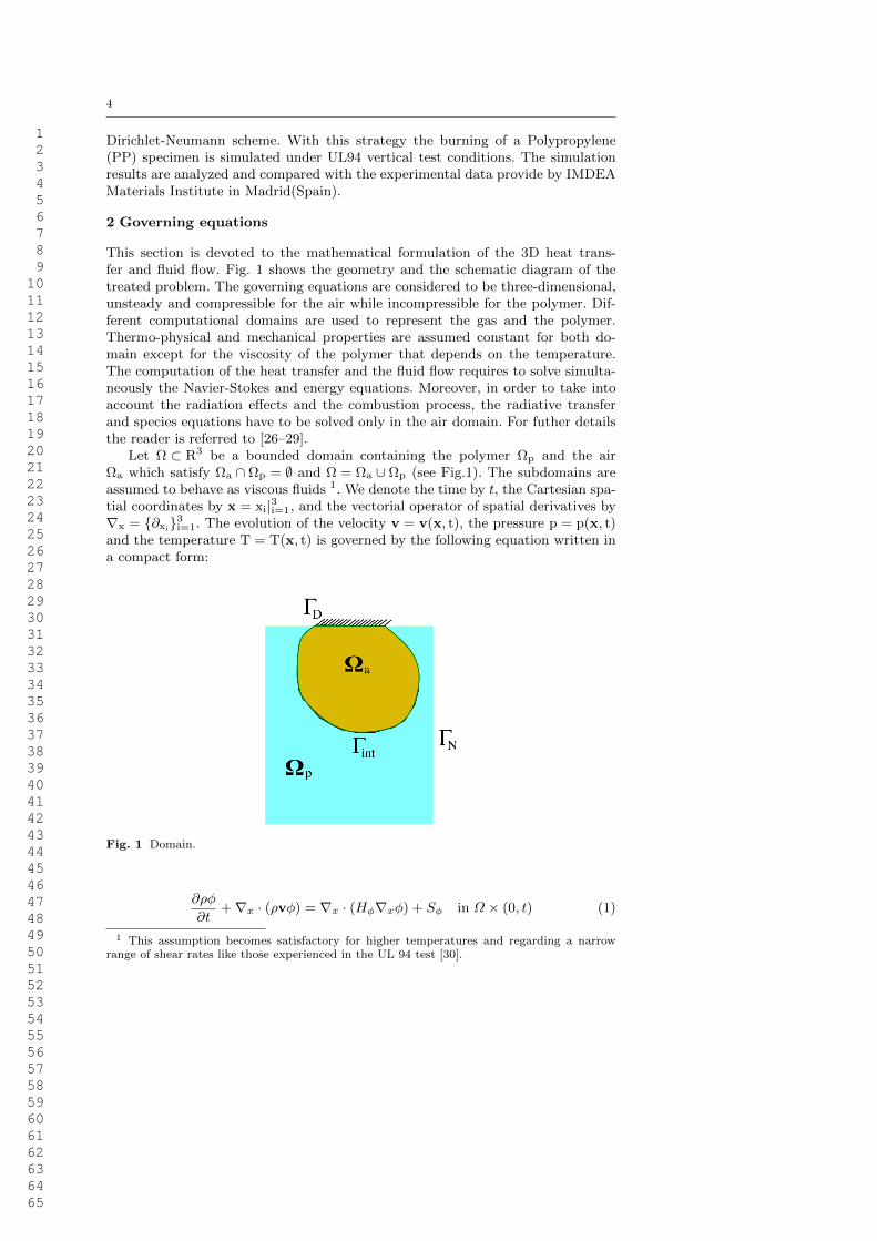
This section is devoted to the mathematical formulation of the 3D heat trans-fer and fluid flow. Fig. 1 shows the geometry and the schematic diagram of thetreated problem. The governing equations are considered to be three-dimensional,unsteady and compressible for the air while incompressible for the polymer. Dif-ferent computational domains are used to represent the gas and the polymer.Thermo-physical and mechanical properties are assumed constant for both do-main except for the viscosity of the polymer that depends on the temperature.The computation of the heat transfer and the fluid flow requires to solve simulta-neously the Navier-Stokes and energy equations. Moreover, in order to take intoaccount the radiation effects and the combustion process, the radiative transferand species equations have to be solved only in the air domain. For futher detailsthe reader is referred to [26–29].

Let Ω ⊂ R3 be a bounded domain containing the polymer Ωp and the airΩa which satisfy Ωa ∩ Ωp = ∅ and Ω = Ωa ∪ Ωp (see Fig.1). The subdomains areassumed to behave as viscous fluids 1. We denote the time by t, the Cartesian spa-tial coordinates by x = xi|3i=1, and the vectorial operator of spatial derivatives by∇x = ∂xi3i=1. The evolution of the velocity v = v(x, t), the pressure p = p(x, t)and the temperature T = T(x, t) is governed by the following equation written ina compact form:

Fig. 1 Domain.

∂ρφ

∂t+∇x · (ρvφ) = ∇x · (Hφ∇xφ) + Sφ in Ω × (0, t) (1)

1 This assumption becomes satisfactory for higher temperatures and regarding a narrowrange of shear rates like those experienced in the UL 94 test [30].

1 2 3 4 5 6 7 8 9 10 11 12 13 14 15 16 17 18 19 20 21 22 23 24 25 26 27 28 29 30 31 32 33 34 35 36 37 38 39 40 41 42 43 44 45 46 47 48 49 50 51 52 53 54 55 56 57 58 59 60 61 62 63 64 65


In the following table φ, Hφ and Sφ are summarized for the different variables:

Transport of φ Hφ SφMass 1 0 εv (1.1)

Momentum v µ −∇xp+µ

3∇x(∇x · v) + ρf (1.2)

Energy T κ/C wT /C + (∇.QR)/C +Qv/C (1.3)

where µ is the fluid viscosity, ρ is the density, p is the fluid pressure, f is thegravity force, C is the heat capacity, κ is the thermal conductivity, wT is the rateof production of heat 2, QR is the radiative heat flux and εv and Qv are the massloss and heat absorbed due pyrolysis in the polymer, respectively. Note that for thepolymer the terms wT/C + (∇.QR)/C is set to zero. In addition, we shall assumefor the air domain the ideal gas equation of state p = ρ/RT which is the mostcommon case for the compressible flows [31].

Equations (1.1-1.3) are completed with standard Dirichlet and Neumann bound-ary conditions. On the external boundary ∂Ω = ΓD

⋃ΓN, such that ΓD ∩ ΓN = ∅(

v = vT = T

)onΓD (2)(

σ.n = σnk∇T.n = qn

)onΓN (3)

where v and T are the prescribed velocity and temperature respectively, n isthe outer unit normal to ΓN, σn and qn are the prescribed traction vector andnormal heat flux.

On the internal interfaces Γint, the coupling conditions are(JvK = 0JT K = 0

)onΓint (4)(

JσK.n = 0Jk∇T K.n = qR

)onΓint (5)

with n the unit normal to Γint, and JφK represents the jump of a quantity φ acrossthe interface.

Radiation modeling

The effect of radiation is taken into consideration in the energy equation asthe divergence of radiative heat flux i.e. ∇ ·QR. Considering gray assumption andneglecting scattering, term ∇ ·QR is given by

∇ ·QR = α

(4σT 4 −

∫ 4π

0

I (s) ds

)(6)

where I is the spectral intensity at the time of the propagation along the directions with speed c and α is the absorption coefficient. Eq.(6) requires the solution ofthe radiative transfer equations (RTE)

s · ∇I (s) = −αI (s) + ασT 4

π(7)

2 Assuming constant values for the Schmidt (Sc = 1) and Prandtl (Pr = 1) numbers simpli-fied composition and temperature dependent transport properties thus ρD = κ/C

1 2 3 4 5 6 7 8 9 10 11 12 13 14 15 16 17 18 19 20 21 22 23 24 25 26 27 28 29 30 31 32 33 34 35 36 37 38 39 40 41 42 43 44 45 46 47 48 49 50 51 52 53 54 55 56 57 58 59 60 61 62 63 64 65

6

Several methods can be used to solve Eq.(7) as by The Discrete Ordinate Method(DOM[32]) or the P1[29], among others. Adopting the P1 method, the intensityI (s) is approximated as

I (s) =1

4π(G+ 3q · s) (8)

where G =∫ 4π

0I (s) ds is the incident radiation, and q the heat flux. Replacing

Eq.(7) into Eq.(8) makes it possible to simplify the RTE equation so that theincident radiation is computed by solving the following system

−∇ ·(

1

3α∇G

)+ αG = 4ασT 4 (9)

If the surfaces are taken to be diffuse and opaque it can be seen that ([29],p.515), under this approximation, the boundary condition becomes

∂G

∂n= − 3αε

4− 2εG+

3αε

4− 2ε4σT 4 (10)

where ε is the surface emissivity. Eq.10 is known as Marchak boundary condi-tion.

The incident incident radiative heat flux to be prescribed onto the air-polymerinterface Γint (Eq. (5)) for the polymer is calculated as

qR =ε

2(2− ε) (4πIb −G) (11)

Note that radiation is only absorbed at the surface of the polymer as in previousworks [30,23,18,20].

Accounting for the gasification effects

The mass loss (εv) and heat absorbed (Qv) due to the pyrolysis process aremodeled as:

εv = −ρAe−E/RT (12)

Qv = ρHεv (13)

where A is the pre-exponential function, E is the activation energy, R is theuniversal gas constant, T is the absolute temperature expressed in Kelvins and His the enthalpy of vaporization. Note that both terms appear on the right handside of Eqs.(1.1) and (1.3).

Combustion model

It is assumed that after pyrolysis the volatiles are released into the gas phaseand combustion with air to form the flame immediately after they are generated.Following [33], the polymer/air reactive system is modeled as a simplified one-step chemical reaction between the fuel(F) and the oxidizer(O) to generate theproduct(P). In particular the reaction is treated as C3H8+5O2 −→ 3CO2+4H2O.For each specie K (C3H8, O2 and 3CO2 + 4H2O) the following equation is solved,

∂ρYK∂t

+∇ · (ρvYK) = ∇ (κ/C∇YK) + wk/C; (14)

1 2 3 4 5 6 7 8 9 10 11 12 13 14 15 16 17 18 19 20 21 22 23 24 25 26 27 28 29 30 31 32 33 34 35 36 37 38 39 40 41 42 43 44 45 46 47 48 49 50 51 52 53 54 55 56 57 58 59 60 61 62 63 64 65


The source terms are respectively wC3H8= −CBcρ2YFYO exp(−Ta/T ) and wO2

=−swC3H8

. In the air domain, the combustion heat release is introduced as wT =hC3H6

Bcρ2YFYO exp(−Ta/T ) in Eq.(1.3). Values of the parameters are obtained

from [34]

3 Numerical strategy

3.1 Particle Finite Element method for the polymer

In the present work the polymer is modeled using the Particle Finite ElementMethod(PFEM). The PFEM uses an updated Lagrangian framework for describ-ing the governing equations [35]. A finite element mesh discretized the domainwhere the equations are solved in the standard FEM methodology. Mesh nodesare treated as particles that can move freely and even separate from the main fluiddomain according to their velocity. Due to the nodes motion, the finite elementmesh is re-generated using Delaunay triangulation [36]. For further details on thePFEM approach the reader may refer to [25,37–39].

Assuming a nearly-incompressible behavior [40], the discrete version of thegoverning equations (Eq. 1.1-1.3) applying the standard backward Euler methodand the Galerkin approach is

(ρM +∆tµK)vn+1 = ρMvn +∆tGpn +∆tρF +∆tFD (15)

Mpn+1 = Mpn −∆tKDvn+1 (16)

(ρCM +∆tκK)Tn+1 = ρCMTn +∆MQ; (17)

FD denotes the drag force resulting from the interaction between the air flowand the polymer particle:

FD =1

2CDAcs‖va − vp‖ (va − vp) (1/Ω) ; (18)

where CD is the drag coefficient, va and vp are the air and polymer velocitiesrespectively and Acs is the cross sectional area.

The mass M, stiffness K and divergence D matrices are assembled from theelemental contributions as:

Mabij = δij

∫V

NaNbdV (19)

Kabij = δijµ

∫V

∂Na

∂xj

∂Nb

∂xjdV + µ

∫V

∂Na

∂xj

∂Nb

∂xjdV+(

∆tK − 2

3µ

)∫V

∂Na

∂xi

∂Nb

∂xjdV

(20)

Gabi =

∫V

∂Na

∂XiNbdV (21)

1 2 3 4 5 6 7 8 9 10 11 12 13 14 15 16 17 18 19 20 21 22 23 24 25 26 27 28 29 30 31 32 33 34 35 36 37 38 39 40 41 42 43 44 45 46 47 48 49 50 51 52 53 54 55 56 57 58 59 60 61 62 63 64 65

8

fai =

∫V

NabidV (22)

D = GT (23)

where N are the standard linear FE shape functions [41], V is the domainintegration defined by the particles occupying the node position x at t = tn+1

( i.e. xn+1). The superscripts refer to the node indices while the Latin(i and j)subscripts refer to the spatial components. The discrete operators follow the defini-tions given by Eqs. (19-23) which are calculated using the unknown configurationxn+1 according to the updated Lagrangian approach.

The governing system of equations (Eqs.15-17) is non-linear and the discreteoperators must be updated at every non-linear iteration according to the newlyobtained mesh position, which is usually evaluated as xn+1,i = Xn+ ∆t

2 (vn+1,i+vn). In order to avoid this iterative procedure, xn+1 is predicted using an explicitstreamline integration. An extended description of this technique may be consultedin [42,35,43]. Once this algorithm is applied onto all the mesh nodes, the newconfiguration V is obtained by creating a mesh connecting these nodes. Once themesh is generated, the system (Eqs.15-17) is solved and the velocity vn+1, thepressure pn+1 and the temperature Tn+1 are known.

3.2 Finite Element formulation for the air

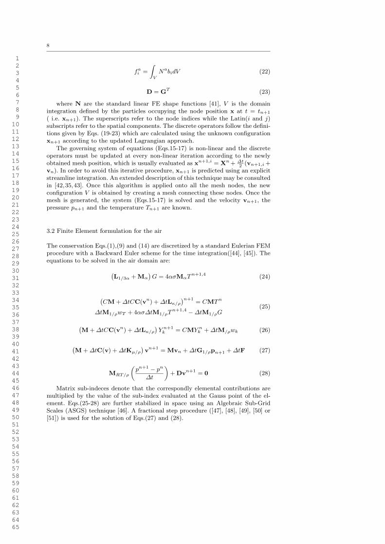
The conservation Eqs.(1),(9) and (14) are discretized by a standard Eulerian FEMprocedure with a Backward Euler scheme for the time integration([44], [45]). Theequations to be solved in the air domain are:(

L1/3α + Mα

)G = 4ασMαT

n+1,4 (24)

(CM +∆tCC(vn) +∆tLκ/ρ

)n+1= CMTn

∆tM1/ρwT + 4ασ∆tM1/ρTn+1,4 −∆tM1/ρG

(25)

(M +∆tCC(vn) +∆tLκ/ρ

)Y n+1k = CMY nk +∆tM/ρwk (26)

(M +∆tC(v) +∆tKµ/ρ

)vn+1 = Mvn +∆tG1/ρpn+1 +∆tF (27)

MRT/ρ

(pn+1 − pn

∆t

)+ Dvn+1 = 0 (28)

Matrix sub-indeces denote that the correspondly elemental contributions aremultiplied by the value of the sub-index evaluated at the Gauss point of the el-ement. Eqs.(25-28) are further stabilized in space using an Algebraic Sub-GridScales (ASGS) technique [46]. A fractional step procedure ([47], [48], [49], [50] or[51]) is used for the solution of Eqs.(27) and (28).

1 2 3 4 5 6 7 8 9 10 11 12 13 14 15 16 17 18 19 20 21 22 23 24 25 26 27 28 29 30 31 32 33 34 35 36 37 38 39 40 41 42 43 44 45 46 47 48 49 50 51 52 53 54 55 56 57 58 59 60 61 62 63 64 65


The discrete operators that correspond to the terms entering the Galerkin partof the weak form are

M =element∑i=1

∫V

NaNbdVi (29)

G =element∑i=1

∫V

∇NaNbdVi (30)

L =element∑i=1

∫V

∇Na∇NbdVi (31)

C(v) =element∑i=1

∫V

Nav · ∇NbdVi (32)

F =element∑i=1

∫V

NaFdVi (33)

Eqs(25,27- 28) represents the implicit version of the explicit strategy presented bythe authors in [23,52]. While in an explicit scheme the density ρn is known duringthe time step, here is unknown and needs to be reevaluated in every iteration.At the beginning of each time step the density is initialized as ρn+1 = ρn and issubsequently updated with the last value of the nonlinear iteration.

4 Overall strategy

The overall solution of the problem involving thermal and mechanical interactionof the polymer and the air can be summarized in the box below

In the polymer:

1. Prescribed in the free surface the normal heat flux qR (Eq.3-Eq.11)provided by the air.

2. Solve energy eq.(Eq.17).3. Solve the polymer motion (Eqs.15-16).

In the air domain:

1. Fix the velocity and temperature (Eq.2) in polymer-air interface fol-lowing [23].

2. Solve RTE(Eq.24).3. Solve energy eq.(air)(Eq.25).4. Solve species eq.(air)(Eq.26).5. Solve the fluid momentum equation (Eqs. 27 -28).

1 2 3 4 5 6 7 8 9 10 11 12 13 14 15 16 17 18 19 20 21 22 23 24 25 26 27 28 29 30 31 32 33 34 35 36 37 38 39 40 41 42 43 44 45 46 47 48 49 50 51 52 53 54 55 56 57 58 59 60 61 62 63 64 65

10

5 Validation model and numerical computation

The burning of a polymer in the UL 94 set up has been modeled numerically withthe strategy proposed in this work. The numerical scheme has been implementedin the open source code KRATOS ([53]). Next we present some details abouthow the PP specimen was prepared as important parameters and data for thenumerical simulation and posteriorly validation by IMDEA Materials Institute.Finally, details of the numerical set up as well as numerical results are presented.

Material and method

The PP specimen (Repsol PP ISPLEN 045 G1E [54]) was prepared using atwin-screw extruder (KETSE 20/40 EC, Brabender) at 200[] and the velocitywas 60 [rpm]. The extruded strands were cut into pellets and then the PP com-posites were injected with an injection molding machine (Arburg 320 C) for furthertests. Complex viscosity of the PP measured with a rheometer (AR2000EX, TAInstruments) at the mode of dynamic temperature step and dynamic frequencysweeping of 0.1 [rad/s], is reported in Fig.2.

Fig. 2 Curve of viscosity

To characterize the thermal degradation and calculate the Arrhenius coeffi-cient and the activation energy a thermogravimetric analysis has been carried outin air using a TGA Q50. The samples were heated with four different heating ratesof 2, 5, 10, 15 [C/min] and the weight loss was measured. The kinetic parame-ters were obtained by methods of Kissinger [55] and Flynn Wall Ozawa (FWO)[56,57]. Activation energy and pre-exponential for the first method are 240.67[KJ/mol] and 7.14× 1016[min−1] while for the second one are 245.62 [KJ/mol]and 1.54× 1016[min−1].

Values for the thermo-physical properties of ρ = 905.0[kg/m3] [54], κ = 0.16[W/mK] and C = 1920[J/kgK] are used as default [58].

A vertical burning test instrument(FTT, U.K.) was used to conduct the testwith sheet dimensions of 148x13x3.2 [mm3] according to ASTM D3801. A flamewas applied at the bottom of the specimen at an angle of 45[].

During the combustion, the temperature was measured and monitored in thecondensed phase with three thermocouples K-type with 0.75[mm] nominal diam-

1 2 3 4 5 6 7 8 9 10 11 12 13 14 15 16 17 18 19 20 21 22 23 24 25 26 27 28 29 30 31 32 33 34 35 36 37 38 39 40 41 42 43 44 45 46 47 48 49 50 51 52 53 54 55 56 57 58 59 60 61 62 63 64 65


eter and 500 [mm] long-Incomel 600 from [59] embedded in the polymer. Thisminiature semi rigid thermocouple was selected due to the response, size, dis-placement and robustness of the assembly. Moreover, this type of thermocouplesis recommended for the cases where the temperature changes are rapid as the pre-sented in this work. More details are provided in [59]. In Fig.4 one can see how theinstrumentation was positioned and fixed. The real time/temperature data wererecorded through a data acquisition apparatus at 0.5[s]. Simultaneously a digitalcamera was used to record the burning process.

Numerical setup and results

In this work, only a fourth part of the polymer is analyzed assuming sym-metrics conditions as in [19]. In the symmetry faces slip and adiabatic boundaryconditions are imposed(Fig.3(a)). The clamping of the sample is modelled by fix-ing the velocities to zero on the top of the specimen. The domain is discretised by100,902 four-noded tetrahedra(see Fig.3(b)). For the air domain, velocity shouldnot be imposed in the inlet since hot temperature in the vicinity of the flamewill increase the buoyancy force and increase locally the air velocity. Howeversuch boundary condition would lead to creation of velocities in some parts of thebottom boundary pointing in the opposite direction(downwards) which leads todivergence of the numerical solver. With the aim of correcting this problem, aconstant uniform velocity is prescribed at the inlet ( vy = 0.2[m/s]). While at thevertical walls slip and adiabatic boundary condition are applied, the top boundaryis defined as a pressure-outlet.

A non-uniform triangular mesh (see Fig.3(b)) formed by 286,850 tetrahedradiscretizes the air domain.

(a) Domains and boundaries conditions (b) Polymer and air meshes

Fig. 3 Problem definition.

1 2 3 4 5 6 7 8 9 10 11 12 13 14 15 16 17 18 19 20 21 22 23 24 25 26 27 28 29 30 31 32 33 34 35 36 37 38 39 40 41 42 43 44 45 46 47 48 49 50 51 52 53 54 55 56 57 58 59 60 61 62 63 64 65

12

(a) View of the set-up. (b) Position of the thermo-couples.

Fig. 4 Position of the thermocouples

The heat flux of the burner in the UL 94 test is applied as an external constantheat flux of 85 [kW/m2]. This is an average value obtained from [19]. The heatflux applied following the criteria presented in[18] during the first 10 [s]. Initially,the gas temperature is set to 298 [K]. The initial fuel and oxygen mass fractionsare 0.0 and 0.23, respectively. Once the sample surface reaches the decompositiontemperature 650[K][60], the value of YF and YO are fixed to 1 and 0 respectively.Regarding thermo-mechanical properties, in the gas phase thermal conductivityκ, the density ρ and the specific heat C are set up to 0.0131 [W/mK], 1.0 [kg/m3]and 1310.0 [J/kgK] [34], respectively while the values of these properties for thepolymer are chosen to be 0.16 [J/kgK], 905.0 [kg/m3] and 1920.0 [W/mK] respec-tively. Note that density changes are described by the ideal gas equation presentedin section 2. The problem was simulated during 100 [s]. The input parameters aresummarized in Table 1.

The viscosity in the air is considered constant while in the polymer it is afunction of temperature. The analytical definition of this curve (see Fig.2 ) corre-sponding to temperatures between 180[C] and 270[C] is given next.

Definition of the viscosity-temperature dependence for the polymer:def AuxFunction(T):if (T > 180.0 and T≤240):mu = 8989008.95× e(−0.015×T)

return mu

For the cases of temperatures below 180[C] and above 270[C] see Fig. 2, viscosityis approximated using the curve provided by NIST and published in [30].

The computed temperature distribution for different time steps across threehorizontal cut planes at different heights of the air domain is presented in Fig.5(a).For the same time steps, the distribution of the fuel is shown in Fig.5(b). Thepresence of fuel is limited to a very thin layer around the polymer-air interface.This is due to the fact that convective transport is more important than the

1 2 3 4 5 6 7 8 9 10 11 12 13 14 15 16 17 18 19 20 21 22 23 24 25 26 27 28 29 30 31 32 33 34 35 36 37 38 39 40 41 42 43 44 45 46 47 48 49 50 51 52 53 54 55 56 57 58 59 60 61 62 63 64 65


diffusive one as a result of the buoyancy forces. Fuel mix with the oxygen andreact with the formation of a flame (see Fig. 5(a)).

From the Figs. it is seen that the heat zone evolves in the air domain givingheat feedback to the polymer. As time progresses the viscosity value decreasesby several orders of magnitude in the polymer. As consequence of the viscositydecrease the sample experiences volume reduction due to melting and drippingtogether with gasification. This starts after a heating time of about 20 [s] and canbe seen in detail in Fig.6.

(a) Temperature distribution

(b) Fuel distribution

Fig. 5 Evolution of the temperature and fuel distribution at time 10, 30 and 50 [s].

1 2 3 4 5 6 7 8 9 10 11 12 13 14 15 16 17 18 19 20 21 22 23 24 25 26 27 28 29 30 31 32 33 34 35 36 37 38 39 40 41 42 43 44 45 46 47 48 49 50 51 52 53 54 55 56 57 58 59 60 61 62 63 64 65

14

0

0.001

0.002

0.003

0.004

0.005

0 20 40 60 80 100

Mas

s[k

g]

Time[s]

ExperimentalNumerical

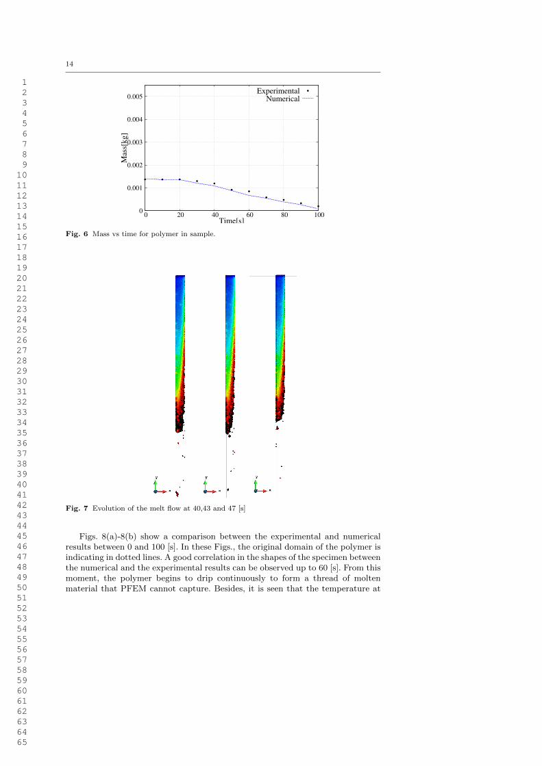
Fig. 6 Mass vs time for polymer in sample.

Fig. 7 Evolution of the melt flow at 40,43 and 47 [s]

Figs. 8(a)-8(b) show a comparison between the experimental and numericalresults between 0 and 100 [s]. In these Figs., the original domain of the polymer isindicating in dotted lines. A good correlation in the shapes of the specimen betweenthe numerical and the experimental results can be observed up to 60 [s]. From thismoment, the polymer begins to drip continuously to form a thread of moltenmaterial that PFEM cannot capture. Besides, it is seen that the temperature at

1 2 3 4 5 6 7 8 9 10 11 12 13 14 15 16 17 18 19 20 21 22 23 24 25 26 27 28 29 30 31 32 33 34 35 36 37 38 39 40 41 42 43 44 45 46 47 48 49 50 51 52 53 54 55 56 57 58 59 60 61 62 63 64 65


the edges is always higher than at the surface center, which is probably due to theedge effect [61,62]. Details of the evolution of the free surface and the melting anddripping can be seen in Fig.7.

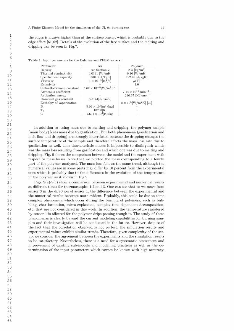
Table 1 Input parameters for the Eulerian and PFEM solvers.

Parameter Air PolymerDensity see Section 2 905 [kg/m3]Thermal conductivity 0.0131 [W/mK] 0.16 [W/mK]Specific heat capacity 1310.0 [J/kgK] 1920.0 [J/kgK]Viscosity 1× 10−5[m2/s] µ(T)Emissivity – 1.0StefanBoltzmann constant 5.67× 10−8[W/m2K4] –Arrhenius coefficient – 7.14× 1016[min−1]Activation energy – 240.67 [KJ/mol]Universal gas constant 8.3144[J/Kmol] –Enthalpy of vaporization – 8× 105[W/m2K] [30]Bc 5.96× 109[m3/kgs] –Ta 10700[K] –C 2.601× 104[Kj/kg] –

In addition to losing mass due to melting and dripping, the polymer sample(main body) loses mass due to gasification. But both phenomena (gasification andmelt flow and dripping) are strongly interrelated because the dripping changes thesurface temperature of the sample and therefore affects the mass loss rate due togasification as well. This characteristic makes it impossible to distinguish whichwas the mass loss resulting from gasification and which one was due to melting anddripping. Fig. 6 shows the comparison between the model and the experiment withrespect to mass losses. Note that we plotted the mass corresponding to a fourthpart of the polymer analyzed. The mass loss follows the same trend, although thenumerical values are in some parts may differ by 10 percent from the experimentalones which is probably due to the differences in the evolution of the temperaturein the polymer as it shown in Fig.9.

Figs. 9(a)-9(c) show a comparison between experimental and numerical resultsat different times for thermocouples 1,2 and 3. One can see that as we move fromsensor 3 in the direction of sensor 1, the difference between the experimental andthe numerical results becomes more evident. Probably, this could be due to somecomplex phenomena which occur during the burning of polymers, such as bub-bling, char formation, micro-explosions, complex time-dependent decomposition,etc. that are not considered in this work. In addition, the temperature registeredby sensor 1 is affected for the polymer drips passing trough it. The study of thesephenomenas is clearly beyond the current modeling capabilities for burning sam-ples and their investigation will be conducted in the future. However, despite ofthe fact that the correlation observed is not perfect, the simulation results andexperimental values exhibit similar trends. Therefore, given complexity of the set-up, we consider the agreement between the experiments and the simulation resultsto be satisfactory. Nevertheless, there is a need for a systematic assessment andimprovement of existing sub-models and modelling practices as well as the de-termination of the input parameters which cannot be known with high accuracy.

1 2 3 4 5 6 7 8 9 10 11 12 13 14 15 16 17 18 19 20 21 22 23 24 25 26 27 28 29 30 31 32 33 34 35 36 37 38 39 40 41 42 43 44 45 46 47 48 49 50 51 52 53 54 55 56 57 58 59 60 61 62 63 64 65

16

(a) T=10, 20, 30, 40 and 50 [s].

(b) T=60, 70, 80, 90 and 100 [s].

Fig. 8 Comparison between experimental versus numerical results.

6 Conclusion

The numerical strategy was developed for modeling of polymers in fire and usedfor reproducing the burning of UL94 test on a simple material (PP).

The numerical results show that the temperature agreed quite well the ten-dency of the temperature measurements given by the three thermocouples locatedinside the condensed phase. Consequently, during specimen combustion, PFEM’sresults show a good agreement with the experimental ones in terms of shape ofthe polymer evolution. Also, the mass loss follows similar trend, although thenumerical values in some locations may differ from the experimental ones.

Although the model shows some deviation from the experimental results andneeds further improvement in the future, one must note that unfortunally up-to-date there exists no other numerical tool to simulate the melting and dripping ofpolymers and compare both results. In this sense, this work makes a new step inthis direction as at least qualitatively the proposed strategy is capable of repro-ducing the test much more accurately than in the previous works dedicated tothe same problem. Thus, the air modelling including a combustion and radiationmodels avoids to estimate a priori not only the value of the flame heat feedbackbut also where and how this need to be distributed along the polymer.

Although the model clearly requires several physical parameters to be deter-mined, in order to ”predict” a very well-known behavior, many of them have

1 2 3 4 5 6 7 8 9 10 11 12 13 14 15 16 17 18 19 20 21 22 23 24 25 26 27 28 29 30 31 32 33 34 35 36 37 38 39 40 41 42 43 44 45 46 47 48 49 50 51 52 53 54 55 56 57 58 59 60 61 62 63 64 65


300

400

500

600

700

800

900

1000

1100

1200

0 20 40 60 80 100 120 140 160 180

Tem

per

atu

re[K

]

Time[s]


(a) Sensor 1

300

400

500

600

700

800

900

1000

1100

1200

0 20 40 60 80 100 120 140 160 180

Tem

per

atu

re[K

]

Time[s]


(b) Sensor 2

300

400

500

600

700

800

900

1000

1100

1200

0 20 40 60 80 100 120 140 160 180

Tem

per

atu

re[K

]

Time[s]


(c) Sensor 3

Fig. 9 Temperature evolution for sensors 1,2 and 3.

been obtained from different literature sources and diverse manufacturers. Thetemperature-dependent values determined for the viscosity of PP enabled PFEMto predict the dripping behavior in the UL 94 scenario. Nevertheless, a bettercharacterization of the chemical reaction in the air and material properties as afunction of temperature are needed to further improve the model. However, itis important to note that inclusion of temperature-dependent parameters is triv-

1 2 3 4 5 6 7 8 9 10 11 12 13 14 15 16 17 18 19 20 21 22 23 24 25 26 27 28 29 30 31 32 33 34 35 36 37 38 39 40 41 42 43 44 45 46 47 48 49 50 51 52 53 54 55 56 57 58 59 60 61 62 63 64 65

18

ial inside our model. Therefore, in case of obtaining these dependencies from theexperimentalists they can be immediately integrated in the model.

With this model the effects of model parameters on UL 94 test scenario could bestudied through varying the value of a single parameter. Therefore, the importanceof each parameter could be quantitatively evaluated. In addition, our numericaltool can be used for improving understanding of the complex burning behaviourincluding the dripping as the competition and interaction of gasification, flameinhibition and removal of fuel and heat from the pyrolysis zone by dripping.

In future work, it would be of interest to use the numerical tool for the predic-tion of flame spread and heat release rate in complex polymer geometries, modelingof standardized fire tests ranging from small scale tests to large-scale tests, andbetter understanding of flammability of anisotropic materials such as composites,and compare it with experiments carry out at larger scale.

References

1. Stoliarov S.I. and Lyon R.E. Thermo-kinetic model of burning for pyrolyzing materials.Fire Safety Science, page 11411152, 2008.

2. Lautenberger C. and Fernndez-Pello C. Generalized pyrolysis model for combustible solids.Fire Safety, 44:819839, 2009.

3. Lautenberger C. Gpyro3d: A three dimensional generalized pyrolysis model. Fire SafetyScience, 11:193–207, 2014.

4. Firefoam code. http://www.fmglobal.com/modeling.5. McGrattan K., McDermott R., Weinschenk C., and Forney G. Fire dynamics simulator

(version 6),technical reference guide, 2013.6. Stoliarov Stanislav I., Leventon Isaac T., and Lyon Richard E. Twodimensional model of

burning for pyrolyzable solids. Fire and Materials, 38(3):391–408, 2013.7. Lautenberger C. and Fernandez-Pello C. A model for the oxidative pyrolysis of wood.

Combustion and Flame, 156(8):1503 – 1513, 2009.8. Lautenberger C., Rein G., and Fernandez-Pello C. The application of a genetic algorithm

to estimate material properties for fire modeling from bench-scale fire test data. FireSafety Journal, 41(3):204 – 214, 2006.

9. Chaos M., Khan M., Krishnamoorthy N., de Ris J., and Dorofeev S. Evaluation of op-timization schemes and determination of solid fuel properties for cfd fire models usingbench-scale pyrolysis tests. Proceedings of the Combustion Institute, 33(2):2599 – 2606,2011.

10. Ramroth W.T., Krysl P., and R.J. Asaro. Sensitivity and uncertainty analyses for fethermal model of frp panel exposed to fire. Composites, Part A 37, 2006.

11. Linteris G.T. Numerical simulations of polymer pyrolysis rate: effect of property variations.Fire and Materials, 35:463480, 2011.

12. Stoliarov S.I., Safronava N., and Lyon R.E. The effect of variation in polymer propertieson the rate of burning. Fire and Materials, 33:257271, 2009.

13. Bal N. and Rein G. Relevant model complexity for non-charring polymer pyrolysis. FireSafety Journal, 61:36 – 44, 2013.

14. C.Di Blasi, S. Crescitelli, G. Russo, and G. Cinque. Numerical model of ignition pro-cesses of polymeric materials including gas-phase absorption of radiation. Combustionand Flame, 83(3):333 – 344, 1991.

15. Tsai T., Li M., Shih I., Jih R., and Wong S. Experimental and numerical study of au-toignition and pilot ignition of pmma plates in a cone calorimeter. Combustion and Flame,124(3):466 – 480, 2001.

16. Wu K., Fan W., Chen C., Liou T., and Pan I. Downward flame spread over a thick pmmaslab in an opposed flow environment: experiment and modeling. Combustion and Flame,132(4):697 – 707, 2003.

17. Gotoda H., Manzello S., Saso Y., and Kashiwagi T. Effects of sample orientation onnonpiloted ignition of thin poly(methyl methacrylate) sheets by a laser: 2. experimentalresults. Combustion and Flame, 145(4):820 – 835, 2006.

1 2 3 4 5 6 7 8 9 10 11 12 13 14 15 16 17 18 19 20 21 22 23 24 25 26 27 28 29 30 31 32 33 34 35 36 37 38 39 40 41 42 43 44 45 46 47 48 49 50 51 52 53 54 55 56 57 58 59 60 61 62 63 64 65


18. Kempel F., Schartel B., Marti J., Butler K., Rossi R., Idelsohn S.R., Onate E., and Hof-mann A. Modelling the vertical ul 94 test: competition and collaboration between meltdripping, gasification and combustion. Fire and Materials, 39(6):570–584, 2015. FAM-14-012.

19. Wang Y., Jow J., Su K., and Zhang J. Development of the unsteady upward fire model tosimulate polymer burning under ul 94 vertical test conditions. Fire Safety Journal, 54:1 –13, 2012. Part of special issue: Large Outdoor Fires.

20. Matzen M., Marti J., Onate E., Idelsohn S., and Schartel B. Advanced experiments andparticle finite element modelling on dripping v-0 polypropylene, fire and materials 2017,15th international conference, san francisco, ca, usa, 2017.

21. Li J. and Stoliarov S.I. Measurement of kinetics and thermodynamics of the thermaldegradation for non- charring polymers. Combust. Flame, 160:1287–1297, 2013.

22. Stoliarov S.I., Safronava N., and Lyon R. E. The effect of variation in polymer propertieson the rate of burning. Fire Mater, 33:257–271, 2009.

23. Marti J., Ryzhakov P., Idelsohn S., and Onate E. Combined eulerian-pfem approach foranalysis of polymers in fire situations. Int. J. Numer. Meth. Engng., 92:782–801, 2010.

24. Onate E., Marti J., Ryzhakov P., Rossi R., and Idelsohn S. Analysis of the melting,burning and flame spread of polymers with the particle finite element method. Computerassisted methods in engineering and science, 20:165 – 184, 2013.

25. Idelsohn S., Onate E., and Del Pin F. The Particle Finite Element Method: a powerfultool to solve incompressible flows with free-surfaces and breaking waves. InternationalJournal of Numerical Methods in Engineering, 61:964–989, 2004.

26. Oliver X. and Agelet de Saracibar C. In Continuum Mechanics for Engineers. Theory andProblems. 2017.

27. Holzapfel G. In Nonlinear Solid Mechanics: A Continuum Approach for Engineering.Wiley, 2000.

28. In Cox G., editor, Combustion Fundamentals of Fire. Academic Press, 1995.29. Modest M.F. Radiative heat transfer. Academic Press, 2003.30. Onate E., Rossi R., Idelsohn S.R., and Butler K. Melting and spread of polymers in fire

with the particle finite element method. International Journal for Numerical Methods inEngineering, 81:1046 – 1072, 2009.

31. Codina R., Vazquez M., and Zienkiewizc O.C. A general algorithm for compressible andincompressible flows. International Journal for Numerical Methods in Fluids, 27:13–32,1998.

32. Fiveland W. The selection of discrete ordinate quadrature sets for anisotropic scattering,asme htd. fundam. radiat. Heat Transfer, 160:89–96, 1991.

33. Sousa Pessoa De Amorim M.T., Comel C., and Vermande P. Pyrolysis of polypropylene.Journal of Analytical and Applied Pyrolysis, 4(1):73 – 81, 1982.

34. Xie W. and DesJardin P. An embedded upward flame spread model using 2d directnumerical simulations. Combustion and Flame, 156(2):522 – 530, 2009.

35. Idelsohn S.R., Marti J., Limache A., and Onate E. Unified lagrangian formulation forelastic solids and incompressible fluids: Application to fluidstructure interaction problemsvia the pfem. Computer Methods in Applied Mechanics and Engineering, 197(19):1762 –1776, 2008. Computational Methods in FluidStructure Interaction.

36. Delaunay B. Sur la sphre vide. izvestia akademii nauk sssr. Otdelenie Matematicheskikhi Estestvennykh Nauk, 7:793–800, 1934.

37. Idelsohn S. R., Marti J., Souto-Iglesias A., and Onate E. Interaction between an elasticstructure and free-surface flows: experimental versus numerical comparisons using thepfem. Computational Mechanics, 43(1):125–132, Dec 2008.

38. Idelsohn S. R., Mier-Torrecilla M., Marti J., and Onate E. The particle finite elementmethod for multi-fluid flows. In Eugenio Onate and Roger Owen, editors, Particle-BasedMethods: Fundamentals and Applications, pages 135–158. Springer Netherlands, Dor-drecht, 2011.

39. Onate E., Idelsohn S. R., Celigueta M. A., Rossi R., Marti J., Carbonell J. M., Ryzhakov P.,and Suarez B. Advances in the particle finite element method (pfem) for solving coupledproblems in engineering. In Eugenio Onate and Roger Owen, editors, Particle-BasedMethods: Fundamentals and Applications, pages 1–49. Springer Netherlands, Dordrecht,2011.

40. Kundu P.K. and Cohen I.M. Fluid mechanics. Academic Press, 2002.41. Hughes T.J.R. The finite element method: Linear static and dynamic finite element anal-

ysis. Computer-Aided Civil and Infrastructure Engineering, 4(3):245–246, 1989.

1 2 3 4 5 6 7 8 9 10 11 12 13 14 15 16 17 18 19 20 21 22 23 24 25 26 27 28 29 30 31 32 33 34 35 36 37 38 39 40 41 42 43 44 45 46 47 48 49 50 51 52 53 54 55 56 57 58 59 60 61 62 63 64 65

20

42. Idelsohn S.R., Nigro N., Gimenez J.M., Rossi R., and Marti J. A fast and accuratemethod to solve the incompressible navier-stokes equations. Engineering Computations,30(2):197–222, 2013.

43. Ryzhakov P.B., Marti J., Idelsohn S.R., and Onate E. Fast fluidstructure interaction simu-lations using a displacement-based finite element model equipped with an explicit stream-line integration prediction. Computer Methods in Applied Mechanics and Engineering,315:1080 – 1097, 2017.

44. Donea J. and Huerta A. Finite element method for flow problems. Wiley, 2003.45. Lohner R. Applied cfd techniques, 2nd edition. J. Wiley and Sons, 2008.46. Codina R. A stabilized finite element method for generalized stationary incompressible

flows. Computer Methods in Applied Mechanics and Engineering, 190(20-21):2681 – 2706,2001.

47. Guermond J.L., Minev P., and Shen J. An overview of projection methods for incompress-ible flows. Computer Methods in Applied Mechanics and Engineering, 195:6011–6045,2006.

48. Temam R. Sur lapproximation de la solution des equations de navier-stokes par la methodedes pase fractionaires. Archives for Rational Mechanics and Analysis, 32:135–153, 1969.

49. Chorin A.J. A numerical method for solving incompressible viscous problems. Journal ofComputational Physics, 2:12–26, 1967.

50. Ryzhakov P. A modified fractional step method for fluid–structure interaction problems.Revista Internacional de Metodos Numericos para Calculo y Diseno en Ingenierıa, 33(1-2):58–64, 2017.

51. Ryzhakov P. and Marti J. A semi-explicit multi-step method for solving incompressiblenavier-stokes equations. Applied Sciences, 8(1), 2018.

52. Ryzhakov P., Rossi R., and Onate E. An algorithm for the simulation of thermally coupledlow speed flow problems. International Journal for Numerical Methods in Fluids, 70(1):1–19, 9 2012.

53. Dadvand P., Rossi R., and Onate E. An object-oriented environment for developing finiteelement codes for multi-disciplinary applications. Archieves of Computational Methods inEngineering, 17/3:253–297, 2010.

54. Repsol pp isplen 045 g1e. http://www.repsol.com/en/products-and-services/chemicals.

55. Kissinger H. Variation of peak temperature with heating rate in differential thermalanalysis. Journal of Research of the National Bureau of Standards, 57(4):217–221, 1956.

56. Flynn J. and Wall L. A quick, direct method for the determination of activation en-ergy from thermogravimetric data. Journal of Polymer Science Part B:Polymer Letters,4(5):323–328, 1966.

57. Ozawa T. A new method of analyzing thermogravimetric data. Bulletin of the ChemicalSociety of Japan, 38:1881–1886, 1965.

58. Thermal properties. http://www.engineeringtoolbox.com/.59. Tc direct. http://www.tcdirect.es/.60. Selected thermal properties. http://pslc.ws/fire/howwhy/thermalp.htm.61. Wang Y., Zhang J., Jow J., and Su K. Analysis and modeling of ignitability of polymers

in the ul-94 vertical burning test condition. J. Fire Sci., 27:561–581, 2009.62. Wang Y., Zhang F., Jiao C., Jin Y., and Zhang J. Convective heat transfer of the bunsen

flame in the ul94 vertical burning test for polymers. J. Fire Sci., 28:337–356, 2010.

1 2 3 4 5 6 7 8 9 10 11 12 13 14 15 16 17 18 19 20 21 22 23 24 25 26 27 28 29 30 31 32 33 34 35 36 37 38 39 40 41 42 43 44 45 46 47 48 49 50 51 52 53 54 55 56 57 58 59 60 61 62 63 64 65

Documents

A Finite Element Model for the simulation of the UL-94