Embed Size (px)
Citation preview
A FINE GRAINED MANY-CORE H.264 VIDEO ENCODER
By
STEPHEN THE UY LEB.S. (Oregon State University) March, 2007
THESIS
Submitted in partial satisfaction of the requirements for the degree of
MASTER OF SCIENCE
in
Electrical and Computer Engineering
in the
OFFICE OF GRADUATE STUDIES
of the
UNIVERSITY OF CALIFORNIA
DAVIS
Approved:
Chair, Dr. Bevan M. Baas
Member, Dr. Venkatesh Akella
Member, Dr. Soheil Ghiasi
Committee in charge2010
– i –


c© Copyright by Stephen The Uy Le 2010All Rights Reserved

Abstract
Video encoding has become an integral part for everyday computing from televisions and computers
to portable devices such as cell phones. Achieving high quality resolution over limited bandwidth
has lead to the development of the H.264 video standard providing greater encoding performance.
In this work an H.264 baseline video encoder is presented on a fine grained 167-core programmable
processor allowing for greater flexibility and parallelization. The encoderpresented is capable of
encoding QCIF-resolution video at 1.00 GHz while dissipating an average of 438 mW, and CIF-
resolution at 1.20 GHz while an average of 787 mW. The Asynchronous Array of Simple Proces-
sors (AsAP) platforms provides a new method of coding over a large number of simple processors
allowing for a higher level of parallelization than digital signal processors(DSP) while avoiding the
complexity of a fully application specific integrated circuit (ASIC).
– ii –

Acknowledgments
I would like to take this chance to thank to everyone that made this work possible. First
I would like to thank Professor Baas for his time, guidance, and support throughout my years at
Davis. The lessons that I learned here will help me for the rest of my career. I would like to thank
Professor Akella and Professor Ghiasi for their valuable support and time in reviewing my thesis.
Thank you to the University of California Davis for providing this educational institution
for learning and enrichment. Graduate school has opened many more doors for me in the future.
I would also like to thank Zhibin Xiao and Gouri Landge for their previous work on video
encoding and Dean Truong for helping me work on the AsAP chip, without your help it would have
taken me much longer to complete this project. I would also like to thank Henna Huang, Layne Miao
and all of the members of the VCL lab for their help and support throughoutmy project making it
not only a great learning experience but a great place to work.
Lastly I would like to thank my family. To my wife and daughter who put up with me
during these long months, thank you for your support and understanding on those 70+ hours of work
a week. Thank you to my parents and siblings for their encouragement andsupport throughout this
time.
This work was supported by ST Microelectronics; IntellaSys; SRC GRC Grant 1598 and
CSR Grant 1659; UC Micro; NSF Grant 0430090, CAREER Award 0546907 and Grant 0903549;
Intel; and SEM. Any opinions, findings, and conclusions or recommendations expressed in this
material are those of the author and do not necessarily relect the views ofthe National Science
Foundation or any of the sponsors.
– iii –
Contents
Abstract ii
Acknowledgments iii
List of Figures vii
List of Tables x
1 Introduction 11.1 Goals of Parallel Video Encoding . . . . . . . . . . . . . . . . . . . . . . . . . .. 11.2 Project Contributions . . . . . . . . . . . . . . . . . . . . . . . . . . . . . . . . . 11.3 Organization . . . . . . . . . . . . . . . . . . . . . . . . . . . . . . . . . . . . . . 2
2 Overview of Video Encoding and the H.264 Standard 32.1 General Video Encoding Concepts . . . . . . . . . . . . . . . . . . . . . . . .. . 3
2.1.1 Digital Video . . . . . . . . . . . . . . . . . . . . . . . . . . . . . . . . . 42.1.2 Video Format . . . . . . . . . . . . . . . . . . . . . . . . . . . . . . . . . 52.1.3 Macroblock Partitioning . . . . . . . . . . . . . . . . . . . . . . . . . . . 72.1.4 Encoding Motion . . . . . . . . . . . . . . . . . . . . . . . . . . . . . . . 7
2.2 Overview of H.264 . . . . . . . . . . . . . . . . . . . . . . . . . . . . . . . . . . 102.2.1 Encoding Path . . . . . . . . . . . . . . . . . . . . . . . . . . . . . . . . 112.2.2 Profiles . . . . . . . . . . . . . . . . . . . . . . . . . . . . . . . . . . . . 122.2.3 Intra Prediction . . . . . . . . . . . . . . . . . . . . . . . . . . . . . . . . 122.2.4 Inter Prediction . . . . . . . . . . . . . . . . . . . . . . . . . . . . . . . . 162.2.5 Integer Transform and Quantization . . . . . . . . . . . . . . . . . . . . . 182.2.6 Reference Frame Reconstruction . . . . . . . . . . . . . . . . . . . . . . . 232.2.7 Entropy Coding . . . . . . . . . . . . . . . . . . . . . . . . . . . . . . . . 232.2.8 Network Abstraction Layer . . . . . . . . . . . . . . . . . . . . . . . . . . 27
3 Processing Platforms Used for Video Encoding 313.1 Related Work in H.264 Processing . . . . . . . . . . . . . . . . . . . . . . . . . .31
3.1.1 Video Encoding on General Purpose (GP) Processors . . . . . . .. . . . . 323.1.2 Video Encoding on Digital Signal Processors (DSP) . . . . . . . . . . .. 323.1.3 Video Encoding on Application Specific Integrated Circuits . . . . . . . . 33
3.2 Proposed H.264 Video Encoder Platform . . . . . . . . . . . . . . . . . . . .. . . 333.2.1 General Overview of AsAP2 Architecture . . . . . . . . . . . . . . . . . .333.2.2 Dynamic Voltage and Frequency Scaling (DVFS) . . . . . . . . . . . . . . 34
– iv –

3.2.3 Memory Architecture . . . . . . . . . . . . . . . . . . . . . . . . . . . . . 353.2.4 Processor Interconnect . . . . . . . . . . . . . . . . . . . . . . . . . . . .353.2.5 Motion Estimation Accelerator . . . . . . . . . . . . . . . . . . . . . . . . 35
4 Parallel Programming Tools 414.1 Message Passing Interface (MPI) . . . . . . . . . . . . . . . . . . . . . . .. . . . 41
4.1.1 Parallel C/MPI Wrapper . . . . . . . . . . . . . . . . . . . . . . . . . . . 414.1.2 AsAP Arbitrary Mapping Tool . . . . . . . . . . . . . . . . . . . . . . . . 42
4.2 Parallel Programming . . . . . . . . . . . . . . . . . . . . . . . . . . . . . . . . . 454.2.1 Methodology . . . . . . . . . . . . . . . . . . . . . . . . . . . . . . . . . 454.2.2 Pitfalls . . . . . . . . . . . . . . . . . . . . . . . . . . . . . . . . . . . . 49
5 Implementation 535.1 Parallel C Implementation . . . . . . . . . . . . . . . . . . . . . . . . . . . . . . 53
5.1.1 General Overview . . . . . . . . . . . . . . . . . . . . . . . . . . . . . . 535.1.2 Intra Prediction . . . . . . . . . . . . . . . . . . . . . . . . . . . . . . . . 545.1.3 Inter Prediction . . . . . . . . . . . . . . . . . . . . . . . . . . . . . . . . 545.1.4 Integer Transform & Quantization & Entropy Coding . . . . . . . . . . . .555.1.5 Network Abstraction Layer (NAL) . . . . . . . . . . . . . . . . . . . . . . 555.1.6 Reference Frame Reconstruction . . . . . . . . . . . . . . . . . . . . . . . 56
5.2 AsAP Implementation . . . . . . . . . . . . . . . . . . . . . . . . . . . . . . . . 565.2.1 General Overview . . . . . . . . . . . . . . . . . . . . . . . . . . . . . . 565.2.2 Memory Organization . . . . . . . . . . . . . . . . . . . . . . . . . . . . 585.2.3 Control Logic . . . . . . . . . . . . . . . . . . . . . . . . . . . . . . . . . 625.2.4 Intra Prediction . . . . . . . . . . . . . . . . . . . . . . . . . . . . . . . . 645.2.5 Inter Prediction . . . . . . . . . . . . . . . . . . . . . . . . . . . . . . . . 665.2.6 Integer Transform & Quantization & Entropy Coding . . . . . . . . . . . .705.2.7 Network Abstraction Layer (NAL) . . . . . . . . . . . . . . . . . . . . . . 735.2.8 Reference Frame Reconstruction . . . . . . . . . . . . . . . . . . . . . . . 73
6 Results and Analysis 776.1 Metrics for Testing and Analysis . . . . . . . . . . . . . . . . . . . . . . . . . . .776.2 Performance Comparisons . . . . . . . . . . . . . . . . . . . . . . . . . . . . . .796.3 Analysis . . . . . . . . . . . . . . . . . . . . . . . . . . . . . . . . . . . . . . . . 82
6.3.1 Chip Utilization . . . . . . . . . . . . . . . . . . . . . . . . . . . . . . . . 826.3.2 Processor Energy . . . . . . . . . . . . . . . . . . . . . . . . . . . . . . . 826.3.3 Processor Utilization . . . . . . . . . . . . . . . . . . . . . . . . . . . . . 926.3.4 Processor Memory Usage . . . . . . . . . . . . . . . . . . . . . . . . . . 1046.3.5 Communication . . . . . . . . . . . . . . . . . . . . . . . . . . . . . . . . 104
7 Future Work and Conclusion 1137.1 Architecture Enhancements for Parallel Programming . . . . . . . . . . . . .. . . 113
7.1.1 Multiple I/O Chips . . . . . . . . . . . . . . . . . . . . . . . . . . . . . . 1137.1.2 Multiple Input Processors . . . . . . . . . . . . . . . . . . . . . . . . . . 1137.1.3 Local Shared Memory . . . . . . . . . . . . . . . . . . . . . . . . . . . . 114
7.2 Tool Enhancements for Parallel Programming . . . . . . . . . . . . . . . . . .. . 1147.2.1 Arbitrary Mapping Tool For AsAP2 . . . . . . . . . . . . . . . . . . . . . 1147.2.2 Analysis of I/O Traffic . . . . . . . . . . . . . . . . . . . . . . . . . . . . 114
– v –

7.2.3 Enhanced I/O File Operations . . . . . . . . . . . . . . . . . . . . . . . . 1157.3 Additional Encoding Functions on AsAP . . . . . . . . . . . . . . . . . . . . . .. 1157.4 Conclusion . . . . . . . . . . . . . . . . . . . . . . . . . . . . . . . . . . . . . . 116
Bibliography 117
– vi –
List of Figures
2.1 Temporal and spatial sampling . . . . . . . . . . . . . . . . . . . . . . . . . . . . 52.2 Sample frame sizes . . . . . . . . . . . . . . . . . . . . . . . . . . . . . . . . . . 62.3 Various video sampling formats [1] . . . . . . . . . . . . . . . . . . . . . . . . . .82.4 Y component of YUV . . . . . . . . . . . . . . . . . . . . . . . . . . . . . . . . . 82.5 U and V Components of YUV picture . . . . . . . . . . . . . . . . . . . . . . . . 92.6 Macro-block partitioning . . . . . . . . . . . . . . . . . . . . . . . . . . . . . . . 92.7 Difference between two frames . . . . . . . . . . . . . . . . . . . . . . . . . . .. 102.8 H.264 encoder path . . . . . . . . . . . . . . . . . . . . . . . . . . . . . . . . . . 112.9 H.264 profiles . . . . . . . . . . . . . . . . . . . . . . . . . . . . . . . . . . . . . 132.10 Intra 16x16 modes . . . . . . . . . . . . . . . . . . . . . . . . . . . . . . . . . . 142.11 Intra 4x4 blocks . . . . . . . . . . . . . . . . . . . . . . . . . . . . . . . . . . . .152.12 Intra 4x4 modes . . . . . . . . . . . . . . . . . . . . . . . . . . . . . . . . . . . . 162.13 Intra chroma modes . . . . . . . . . . . . . . . . . . . . . . . . . . . . . . . . . . 162.14 Macroblock partition for ME . . . . . . . . . . . . . . . . . . . . . . . . . . . . .172.15 Sample macroblock partition for ME . . . . . . . . . . . . . . . . . . . . . . . . . 182.16 MV prediction from neighboring blocks [1] . . . . . . . . . . . . . . . . . .. . . 192.17 Reorder transform blocks . . . . . . . . . . . . . . . . . . . . . . . . . . . .. . . 202.18 CAVLC zig zag scan . . . . . . . . . . . . . . . . . . . . . . . . . . . . . . . . . 26
3.1 AsAP array . . . . . . . . . . . . . . . . . . . . . . . . . . . . . . . . . . . . . . 343.2 AsAP processor architecture . . . . . . . . . . . . . . . . . . . . . . . . . . .. . 363.3 AsAP nearest neighbor communication . . . . . . . . . . . . . . . . . . . . . . .363.4 ME accelerator block diagram . . . . . . . . . . . . . . . . . . . . . . . . . . . .373.5 ME Accelerator control sequence . . . . . . . . . . . . . . . . . . . . . . . .. . . 383.6 ME accelerator interface . . . . . . . . . . . . . . . . . . . . . . . . . . . . . . .393.7 ME flow diagram . . . . . . . . . . . . . . . . . . . . . . . . . . . . . . . . . . . 39
4.1 C model of encoder in asapmap . . . . . . . . . . . . . . . . . . . . . . . . . . . .434.2 Encoder processors in asapmap . . . . . . . . . . . . . . . . . . . . . . . . .. . . 444.3 Proposed mapping of processors by asapmap . . . . . . . . . . . . . . . .. . . . 464.4 Problems with more than 3 inputs per processor . . . . . . . . . . . . . . . . . .. 484.5 Multiple input problem 3 . . . . . . . . . . . . . . . . . . . . . . . . . . . . . . . 484.6 Solutions for more than 2 inputs per processor . . . . . . . . . . . . . . . . .. . . 504.7 Multiple input solution 3 . . . . . . . . . . . . . . . . . . . . . . . . . . . . . . . 50
5.1 H.264 encoder path for parallel C/MPI implementation . . . . . . . . . . . . . . .54
– vii –

5.2 FPGA-AsAP block diagram . . . . . . . . . . . . . . . . . . . . . . . . . . . . . 575.3 H.264 encoder path - AsAP . . . . . . . . . . . . . . . . . . . . . . . . . . . . . .575.4 H.264 blocks on AsAP . . . . . . . . . . . . . . . . . . . . . . . . . . . . . . . . 585.5 Partition of processor type on AsAP . . . . . . . . . . . . . . . . . . . . . . . .. 595.6 Communication links for AsAP implementation . . . . . . . . . . . . . . . . . . . 605.7 Current/reference frame on AsAP . . . . . . . . . . . . . . . . . . . . . . . .. . 615.8 Macroblock storage in memory . . . . . . . . . . . . . . . . . . . . . . . . . . . . 625.9 High level block diagram of intra prediction in AsAP . . . . . . . . . . . . . . .. 645.10 Intra prediction in AsAP . . . . . . . . . . . . . . . . . . . . . . . . . . . . . . . 655.11 Intra prediction mapping . . . . . . . . . . . . . . . . . . . . . . . . . . . . . . . 675.12 Intra chroma prediction AsAP layout . . . . . . . . . . . . . . . . . . . . . . .. . 685.13 Inter prediction in AsAP . . . . . . . . . . . . . . . . . . . . . . . . . . . . . . . 685.14 ME ACC reference macroblock partition . . . . . . . . . . . . . . . . . . . . . . 695.15 ME diamond search . . . . . . . . . . . . . . . . . . . . . . . . . . . . . . . . . . 705.16 Inter prediction in AsAP block diagram . . . . . . . . . . . . . . . . . . . . . .. 715.17 Layout of inter prediction in AsAP . . . . . . . . . . . . . . . . . . . . . . . . .. 725.18 Block diagram of integer transform and CAVLC . . . . . . . . . . . . . . .. . . . 725.19 Layout of integer transform and CAVLC on AsAP . . . . . . . . . . . . .. . . . . 735.20 Layout of header module on AsAP . . . . . . . . . . . . . . . . . . . . . . . .. . 745.21 Block diagram of reconstruction module . . . . . . . . . . . . . . . . . . . . .. . 745.22 Layout of reconstruction module on AsAP . . . . . . . . . . . . . . . . . . .. . . 75
6.1 Power distribution of major blocks in intra prediction . . . . . . . . . . . . . . . .846.2 Power distribution for major blocks in inter prediction . . . . . . . . . . . . . . .. 846.3 Average power and number of encoded frames per second vs. frequency at 1.3V on
AsAP2 chip . . . . . . . . . . . . . . . . . . . . . . . . . . . . . . . . . . . . . . 856.4 Average power and number of encoded frames per second vs. frequency at 1.2V on
AsAP2 chip . . . . . . . . . . . . . . . . . . . . . . . . . . . . . . . . . . . . . . 866.5 Average power and number of encoded frames per second vs. frequency at 1.1V on
AsAP2 chip . . . . . . . . . . . . . . . . . . . . . . . . . . . . . . . . . . . . . . 876.6 Average power and number of encoded frames per second vs. frequency at 1.0V on
AsAP2 chip . . . . . . . . . . . . . . . . . . . . . . . . . . . . . . . . . . . . . . 886.7 Average power and number of encoded frames per second vs. frequency at 0.9V on
AsAP2 chip . . . . . . . . . . . . . . . . . . . . . . . . . . . . . . . . . . . . . . 896.8 Average power and number of encoded frames per second vs. frequency at 0.8V on
AsAP2 chip . . . . . . . . . . . . . . . . . . . . . . . . . . . . . . . . . . . . . . 906.9 Average power of prediction processors . . . . . . . . . . . . . . . . . .. . . . . 916.10 Average power of reconstruction processors . . . . . . . . . . . . .. . . . . . . . 936.11 Average power of integer transform processors . . . . . . . . . . .. . . . . . . . 946.12 Average power for CAVLC processors . . . . . . . . . . . . . . . . . .. . . . . . 956.13 Average activity of processors used in intra prediction . . . . . . . . .. . . . . . . 966.14 Average Activity of processors used in inter prediction . . . . . . . . .. . . . . . 966.15 Average activity of reconstruction processors . . . . . . . . . . . . .. . . . . . . 976.16 Average activity of integer transorm processors . . . . . . . . . . . .. . . . . . . 986.17 Average activity of CAVLC processors . . . . . . . . . . . . . . . . . . .. . . . . 996.18 Comparison of average activty before and after frequency scaling for intra prediction 1006.19 Frequency of intra prediction processors after frequency scaling . . . . . . . . . . 1016.20 Average power of intra prediction processors after frequency and voltage scaling . 101
– viii –

6.21 Comparison of average activity before and after frequency scaling for inter prediction1026.22 Frequency of inter prediction processors after frequency scaling . . . . . . . . . . 1036.23 Average power of inter prediction processors after frequency and voltage scaling . 1036.24 Number of instruction and data memory words used per processors. Dynamic Mem-
ory (DC Mem) is only listed for memory processors where they are used fordatastorage and computation. . . . . . . . . . . . . . . . . . . . . . . . . . . . . . . . 105
6.25 Number of instruction memory words used per processor . . . . . . . . .. . . . . 1066.26 Instruction memory usage for prediction processors . . . . . . . . . . .. . . . . . 1066.27 Number of instruction memory words used for integer transform, CAVLC, and re-
construction processors . . . . . . . . . . . . . . . . . . . . . . . . . . . . . . . .1076.28 Scatter plot of instruction memory vs. data memory for all processor. . .. . . . . . 1086.29 Scatter plot of instruction and data memory for prediction processors .. . . . . . . 1086.30 Scatter plot of instruction and data memory for integer prediction and CAVLC pro-
cessors . . . . . . . . . . . . . . . . . . . . . . . . . . . . . . . . . . . . . . . . . 1096.31 Average and max throughput of major intra prediction communication links.Link
lenght is determined by the number of intersected processros minus 1. . . . .. . . 1106.32 Average and max throughput of major inter prediction communication links.Link
length is determined by the number of intersected processors minus 1. . . . . .. . 111
– ix –
List of Tables
2.1 Frame rate . . . . . . . . . . . . . . . . . . . . . . . . . . . . . . . . . . . . . . . 42.2 Size of raw video . . . . . . . . . . . . . . . . . . . . . . . . . . . . . . . . . . . 42.3 Sample frame sizes . . . . . . . . . . . . . . . . . . . . . . . . . . . . . . . . . . 52.4 Signed ExpGolomb code table . . . . . . . . . . . . . . . . . . . . . . . . . . . . 242.5 Explicit Exp-Golomb code . . . . . . . . . . . . . . . . . . . . . . . . . . . . . . 242.6 Prefix and suffix for codeNum . . . . . . . . . . . . . . . . . . . . . . . . . .. . 242.7 Coded block pattern mapping . . . . . . . . . . . . . . . . . . . . . . . . . . . . . 242.8 CodeNum for block patterns . . . . . . . . . . . . . . . . . . . . . . . . . . . . .252.9 CAVLC components . . . . . . . . . . . . . . . . . . . . . . . . . . . . . . . . . 252.10 NALU bit field . . . . . . . . . . . . . . . . . . . . . . . . . . . . . . . . . . . . 272.11 PPS fields . . . . . . . . . . . . . . . . . . . . . . . . . . . . . . . . . . . . . . . 282.12 SPS fields . . . . . . . . . . . . . . . . . . . . . . . . . . . . . . . . . . . . . . . 282.13 SH fields . . . . . . . . . . . . . . . . . . . . . . . . . . . . . . . . . . . . . . . . 29
3.1 Encoder performance on Intel Quad Core . . . . . . . . . . . . . . . . . .. . . . 323.2 Encoder preformance on DSP platform . . . . . . . . . . . . . . . . . . . . .. . . 323.3 Encoder performance on ASIC Platform . . . . . . . . . . . . . . . . . . . .. . . 333.4 Power measurements for various configurations on AsAP . . . . . . . . .. . . . . 35
5.1 Output format AsAP . . . . . . . . . . . . . . . . . . . . . . . . . . . . . . . . . 64
6.1 Performance of H.264 video encoder on AsAP2 chip . . . . . . . . . . . .. . . . 806.2 Comparison of H.264 Encoders * These value are interpolated from given data
based on the number of macroblocks that can be encoded per second . .. . . . . . 816.3 Comparison of custom layout and proposed mapping from AsAP arbitrary mapping
tool . . . . . . . . . . . . . . . . . . . . . . . . . . . . . . . . . . . . . . . . . . 826.4 Power consumption of various AsAP instructions as measured in lab usedfor power
calculations in simulation . . . . . . . . . . . . . . . . . . . . . . . . . . . . . . . 83
– x –
1
Chapter 1
Introduction
1.1 Goals of Parallel Video Encoding
Demand for high quality video has become increasingly important in today’s society from
standard applications such as television broadcasting to streaming videos viacell phones. Video is
often stored or transmitted prior to use, because of bandwidth limitations however video must be
encoded for efficient transmission/storage. The computational complexity of this process has led to
many different solutions with application specific processors having great success. Programmable
solutions though flexible are not able to handle the computational load required and have focused
on smaller applications. To achieve high quality video encoding on a small programmable chip,
task and data level parallelism must be exploited at a fine grained level. The goal of this project
is to develop a real-time H.264 video encoder with performance comparable to application specific
processors and the flexibility of programmable processors.
1.2 Project Contributions
Research contributions of this project include:
• An MPI-C Baseline H.264 video encoder
• A real-time H.264 baseline video encoder on a asynchronous array of simple processors
• Thorough performance analysis for parallelization of a H.264 encoder
2 CHAPTER 1. INTRODUCTION
• Thorough processor analysis for a large fine grained application
1.3 Organization
The remainder of this paper is divided as follows. Chapter 2 provides a basic overview
of video encoding and the H.264 video standard. Chapter 3 deals with processing platforms used
for video encoding specifically the asynchronous array of simple processors proposed for this im-
plementation. Chapter 4 discusses some tools, methodologies, and pitfalls of parallel programming.
Chapter 5 presents the proposed implementation. Results, analysis, and comparisons with other
encoders are given in chapter 6. Chapter 7 concludes the paper with possibilities for future work.
3
Chapter 2
Overview of Video Encoding and the
H.264 Standard
Encoding a video sequence has always been a challenge due to the complexity of com-
pressing then reproducing an exact copy of the original file again. As the picture size increases the
problem becomes even greater, requiring more data to be compressed in thesame amount of time.
The H.264 standard [2] provides new encoding techniques yielding greater compression and higher
quality. The standard itself does not present an encoder or decoder but a syntax that must be met
to ensure that an encoded video stream can be decoded on a H.264 compliant decoder. Hence the
syntax given in the standard is defined for the decoding process and anencoder must essentially
produce that same syntax.
The H.264 Standard is a joint development of the Moving Picture Experts Group (MPEG)
and the Video Coding Experts Group (VCEG) released by the International Telecommunication
Union (ITU) Telecommunication Standardization Sector (ITU-T) as H.264 and Part 10 of MPEG-4.
2.1 General Video Encoding Concepts
Video sequences are a series of still pictures (referred to as frames from this point forward)
that are flashed at a high rate to give the impression that objects in the pictures are moving. In most
applications this requires approximately 25 frames per second (fps). Because of the high sampling
rate, the difference between each successive frame is relatively small, hence if only the difference
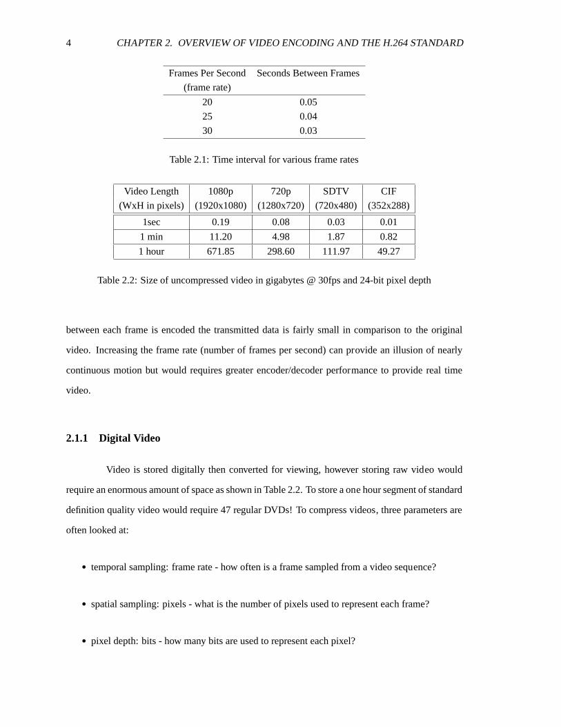
4 CHAPTER 2. OVERVIEW OF VIDEO ENCODING AND THE H.264 STANDARD
Frames Per Second Seconds Between Frames
(frame rate)
20 0.05
25 0.04
30 0.03
Table 2.1: Time interval for various frame rates
Video Length 1080p 720p SDTV CIF
(WxH in pixels) (1920x1080) (1280x720) (720x480) (352x288)
1sec 0.19 0.08 0.03 0.01
1 min 11.20 4.98 1.87 0.82
1 hour 671.85 298.60 111.97 49.27
Table 2.2: Size of uncompressed video in gigabytes @ 30fps and 24-bit pixel depth
between each frame is encoded the transmitted data is fairly small in comparison tothe original
video. Increasing the frame rate (number of frames per second) can provide an illusion of nearly
continuous motion but would requires greater encoder/decoder performance to provide real time
video.
2.1.1 Digital Video
Video is stored digitally then converted for viewing, however storing raw video would
require an enormous amount of space as shown in Table 2.2. To store a one hour segment of standard
definition quality video would require 47 regular DVDs! To compress videos, three parameters are
often looked at:
• temporal sampling: frame rate - how often is a frame sampled from a video sequence?
• spatial sampling: pixels - what is the number of pixels used to represent each frame?
• pixel depth: bits - how many bits are used to represent each pixel?

2.1. GENERAL VIDEO ENCODING CONCEPTS 5
Spatial Samples
Temporal Samples
Figure 2.1: Temporal and spatial sampling
Format Horizontal x Vertical Pixels per Frame Ratio of Pixels per Frame
Resolution (4:2:0 Format) Compared to SDTV
Sub-QCIF 128x96 12288 .02 : 1.0
Quarter CIF 176x144 38016 .06 : 1.0
CIF 352x288 152064 .25 : 1.0
4CIF (SDTV) 704x576 608256 1.0 : 1.0
720p 1280x720 1382400 2.3 : 1.0
1080p 1920x1080 2073600 3.4 : 1.0
Table 2.3: Sample of various frame sizes
2.1.2 Video Format
Various video formats are used depending on the quality of the video needed, smaller
formats are more compact and require less space to store but do not provide very high quality
resolution; larger formats allow for more detail but require more storage space, and consequentially
more computational power to encode. The Common Intermediate Format (CIF) and smaller ones
are commonly used for streaming type applications, such as mobile devices. 4CIF is often used
for standard definition televisions (SDTV) and DVD-videos, and 720p (720 lines of progressively
scanned data) or 1080p is commonly used for High Definition (HD) quality video. Table 2.3 and
Fig. 2.2 give a comparison of some common video formats, larger ones are ofcourse possible simply
by increasing the horizontal and vertical resolution of each frame.

6 CHAPTER 2. OVERVIEW OF VIDEO ENCODING AND THE H.264 STANDARD
Figure 2.2: Different frame sizes for digital video [1]
RGB
The pictures in Fig. 2.2 are shown in black and white where each spatial sample is rep-
resented by one value giving the brightness of the pixel. To represent color images at least three
values are required per pixel. One of the common methods of representing this color space is the
RGB format where Red, Blue, and Green are each represented by onenumber giving the brightness
desired, when combined together these three primary colors can create any other color.
YCbCr (YUV)
Another common format YCbCr(commonly referred to as YUV) takes advantage of the
fact that the human eye is more sensitive to brightness than color, that is we can notice slight changes
in light and dark easier than different shades of a color. In RGB formateach color is represented
equally, to get every pixel in color requires 3 values per pixel. In the YUVformat the bright-
ness/luminance (luma) is separated from the color (chroma) so that each can be given a different
weight. One variable (Y) determines the luminance component, and two variables U and V give the
chrominance of each pixel. The conversion between RGB and YUV formatcan be done using the
simplified equations (2.1) recommended by the ITU-R.
2.1. GENERAL VIDEO ENCODING CONCEPTS 7
R = Y + 1.402Cr
G = Y − 0.344Cb − 0.714Cr
B = Y + 1.772Cb (2.1)
Sampling Formats
Various sampling format for YUV give different weights to the luma and chroma com-
ponents. Full sampling (referred to as 4:4:4) gives equal weight to all three, similar to RGB, this
format requires 3 values to represent each pixel. The 4:2:2 format gives the chroma components
half the weight of the luma components. For each 4x4 block of luma pixels, the chroma component
is represented with the same weight in the vertical direction but half the weightin the horizontal
position, that is every other column is represented with both luma and chroma components, and the
intermediate columns are only represented by luma components. The 4:4:4 and 4:2:2 formats are
generally used for high quality color videos. The more popular 4:2:0 formatused in this paper gives
chroma one quarter the resolution of the luma component. As shown in Fig. 2.3(a), for each 4x4
block of luma pixels there is only one U and V component. Also note that the numbering scheme
for 4:2:0 does not necessarily correspond to representations and directions.
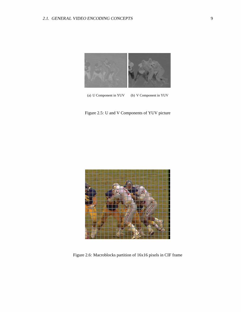
2.1.3 Macroblock Partitioning
In sampling video frames, pixels are grouped into blocks of 16x16 to form amacroblock.
Figure 2.6 shows the partition of macroblocks on a CIF video frame. Encoding is done on a mac-
roblock basis with macroblock 0 in the top left corner and the last macroblockin the bottom right.
For the 4:2:0 format, each 16x16 (256 pixels) luma macroblock corresponds to two 8x8 (64 pixels)
chroma block. Within each macroblock the pixels are ordered starting with index 0 in the top left
corner and 255 in the bottom right corner.
2.1.4 Encoding Motion
Between each successive frame there is relatively little differences in motion. Generally
it is from either the camera panning/moving or from some object/person moving,Fig. 2.7 shows

8 CHAPTER 2. OVERVIEW OF VIDEO ENCODING AND THE H.264 STANDARD
(a) 4:2:0 format (b) 4:2:2 format
(c) 4:4:4 format
Figure 2.3: Various video sampling formats [1]
Figure 2.4: Y component of YUV picture
2.1. GENERAL VIDEO ENCODING CONCEPTS 9
(a) U Component in YUV (b) V Component in YUV
Figure 2.5: U and V Components of YUV picture
Figure 2.6: Macroblocks partition of 16x16 pixels in CIF frame

10 CHAPTER 2. OVERVIEW OF VIDEO ENCODING AND THE H.264 STANDARD
(a) frame 0 (b) frame 1 (c) frame 1 - frame 0
(d) Y component of differ-
ence
(e) U component of differ-
ence
(f) V component of difference
Figure 2.7: Difference between two frames
two successive frames with the bright spots in Fig. 2.7(c) showing the difference. To determine the
difference between each frame, each macroblock (16x16 square of pixels) is compared to a similar
area in a previous frame to find the closest match. One method is to overlay the two regions then
do direct subtraction to find the sum of absolute differences (SAD) for that position, the current
macroblock is then moved one pixel in any direction and the SAD is recalculated. Once this is done
a certain number of times, the position with the minimum SAD is chosen to be encoded.Since
there is little motion between frames due to the high frame rate, the search area can generally be
limited to a small area. If two frames are uncorrelated (have no similarities) the SAD will be much
greater, this will only generate more data to be encoded but will not affectthe accuracy/quality of
the decoded picture.
2.2 Overview of H.264
The H.264 standard defines a syntax for decoding a compressed video,in this work an
encoder perspective will be taken. The encoding process should matchthe decoding process as close
as possible to ensure quality video compression and decompression. For adetailed explanation of
2.2. OVERVIEW OF H.264 11
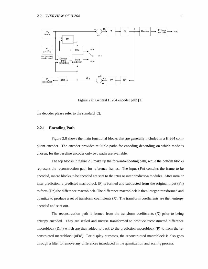
Figure 2.8: General H.264 encoder path [1]
the decoder please refer to the standard [2].
2.2.1 Encoding Path
Figure 2.8 shows the main functional blocks that are generally included in a H.264 com-
pliant encoder. The encoder provides multiple paths for encoding depending on which mode is
chosen, for the baseline encoder only two paths are available.
The top blocks in figure 2.8 make up the forward/encoding path, while the bottom blocks
represent the reconstruction path for reference frames. The input (Fn) contains the frame to be
encoded, macro blocks to be encoded are sent to the intra or inter prediction modules. After intra or
inter prediction, a predicted macroblock (P) is formed and subtracted fromthe original input (Fn)
to form (Dn) the difference macroblock. The difference macroblock is then integer transformed and
quantize to produce a set of transform coefficients (X). The transform coefficients are then entropy
encoded and sent out.
The reconstruction path is formed from the transform coefficients (X) prior to being
entropy encoded. They are scaled and inverse transformed to produce reconstructed difference
macroblock (Dn’) which are then added to back to the prediction macroblock(P) to from the re-
constructed macroblock (uFn’). For display purposes, the reconstructed macroblock is also goes
through a filter to remove any differences introduced in the quantization andscaling process.
12 CHAPTER 2. OVERVIEW OF VIDEO ENCODING AND THE H.264 STANDARD
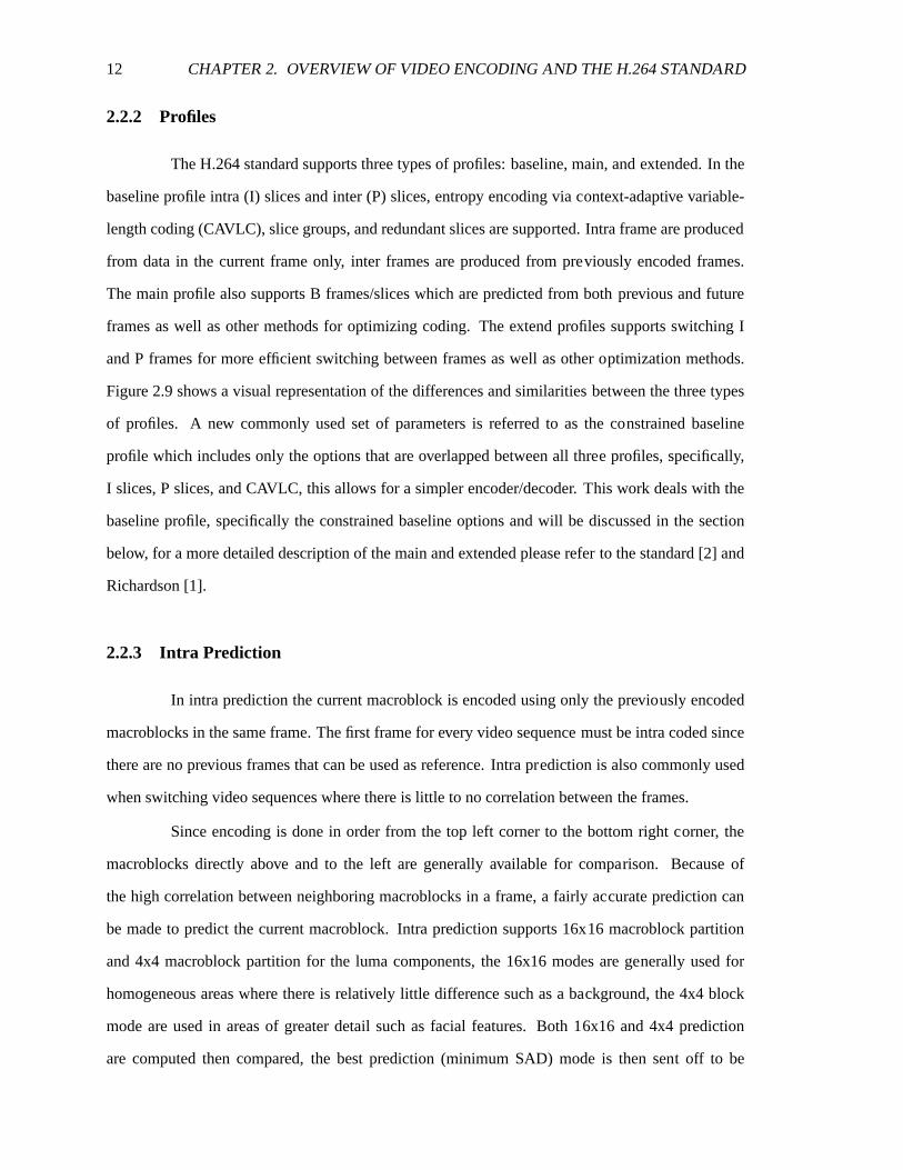
2.2.2 Profiles
The H.264 standard supports three types of profiles: baseline, main, andextended. In the
baseline profile intra (I) slices and inter (P) slices, entropy encoding via context-adaptive variable-
length coding (CAVLC), slice groups, and redundant slices are supported. Intra frame are produced
from data in the current frame only, inter frames are produced from previously encoded frames.
The main profile also supports B frames/slices which are predicted from bothprevious and future
frames as well as other methods for optimizing coding. The extend profiles supports switching I
and P frames for more efficient switching between frames as well as other optimization methods.
Figure 2.9 shows a visual representation of the differences and similaritiesbetween the three types
of profiles. A new commonly used set of parameters is referred to as the constrained baseline
profile which includes only the options that are overlapped between all three profiles, specifically,
I slices, P slices, and CAVLC, this allows for a simpler encoder/decoder. This work deals with the
baseline profile, specifically the constrained baseline options and will be discussed in the section
below, for a more detailed description of the main and extended please referto the standard [2] and
Richardson [1].
2.2.3 Intra Prediction
In intra prediction the current macroblock is encoded using only the previously encoded
macroblocks in the same frame. The first frame for every video sequencemust be intra coded since
there are no previous frames that can be used as reference. Intra prediction is also commonly used
when switching video sequences where there is little to no correlation betweenthe frames.
Since encoding is done in order from the top left corner to the bottom right corner, the
macroblocks directly above and to the left are generally available for comparison. Because of
the high correlation between neighboring macroblocks in a frame, a fairly accurate prediction can
be made to predict the current macroblock. Intra prediction supports 16x16 macroblock partition
and 4x4 macroblock partition for the luma components, the 16x16 modes are generally used for
homogeneous areas where there is relatively little difference such as a background, the 4x4 block
mode are used in areas of greater detail such as facial features. Both 16x16 and 4x4 prediction
are computed then compared, the best prediction (minimum SAD) mode is then sent off to be
2.2. OVERVIEW OF H.264 13
Figure 2.9: H.264 profiles [1]

14 CHAPTER 2. OVERVIEW OF VIDEO ENCODING AND THE H.264 STANDARD
Figure 2.10: Prediction modes for intra 16x16 macroblock partition [1]
encoded. A predicted value for each pixel is first determined dependingon the mode, this value is
then subtracted from the current pixel to get the residue which will be encoded.
16x16 Prediction
In intra 16x16 luma prediction, four modes are possible, vertical, horizontal, DC, and
plane. All four modes are computed to determine the closes match (least amountof residue -
minimum SAD), the best mode is then chosen for comparison with intra 4x4 luma prediction. In
vertical prediction, the predicted value is taken from the last row of the above macroblock (H),
shown in Fig. 2.10, hence for every pixel in that column the same predicted value is used. In
horizontal prediction, the predicted value is taken from the right most columnof the left neighboring
macroblock in the same row (V), as with vertical prediction, the same predictedvalue is used for
the entire row, and is subtracted from the current pixel. In DC prediction,the average of last row of
the above macroblock and the right most column of the left macroblock values(H+V)are taken to
be the predicted value, if either of above or left data is unavailable, the predicted value for that side
is take to be 2̂(bit depth-1) (for a bit depth of 8, this is 128), hence this mode can always beused for
prediction. In DC prediction mode, the same predicted number is used for the entire block. In plane
mode a linear plane function is generated from the upper and left samples (H, V) with different
predicted values depending on the location.
4x4 Prediction
In intra 4x4 luma prediction the four modes from intra 16x16 prediction are available as
well as five additional modes. The 16x16 macroblock is divided into four rows and four columns
2.2. OVERVIEW OF H.264 15
1 6 P i x e l s
1 6 P i x e l s
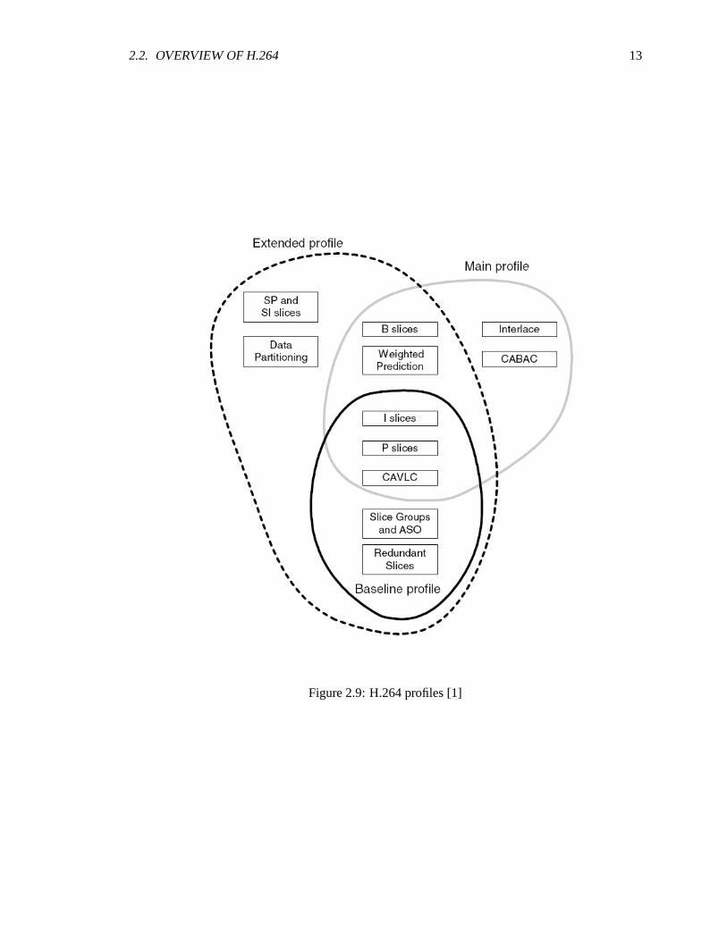
4 x 4B l o c k 0 4 x 4B l o c k 1 4 x 4B l o c k 2 4 x 4B l o c k 34 x 4B l o c k 4 4 x 4B l o c k 5 4 x 4B l o c k 6 4 x 4B l o c k 74 x 4B l o c k 8 4 x 4B l o c k 9 4 x 4B l o c k 1 0 4 x 4B l o c k 1 14 x 4B l o c k 1 2 4 x 4B l o c k 1 3 4 x 4B l o c k 1 4 4 x 4B l o c k 1 5Figure 2.11: Partition for intra 4x4 macroblocks
producing 16 blocks 4 pixels tall by 4 pixels wide as shown in Fig. 2.11. The best mode for each
4x4 block is first determined, once this is done the total SAD for all 16 blocksare compared with
the 16x16 prediction mode to determine the best one. Values used for prediction are computed from
either the above and left macroblock if the current 4x4 block lies on an edge (blocks 0-3, 4, 8, or 12),
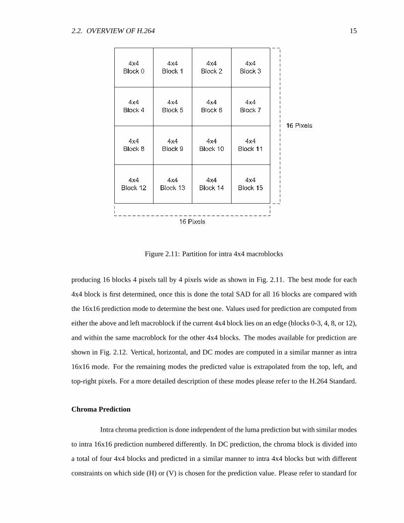
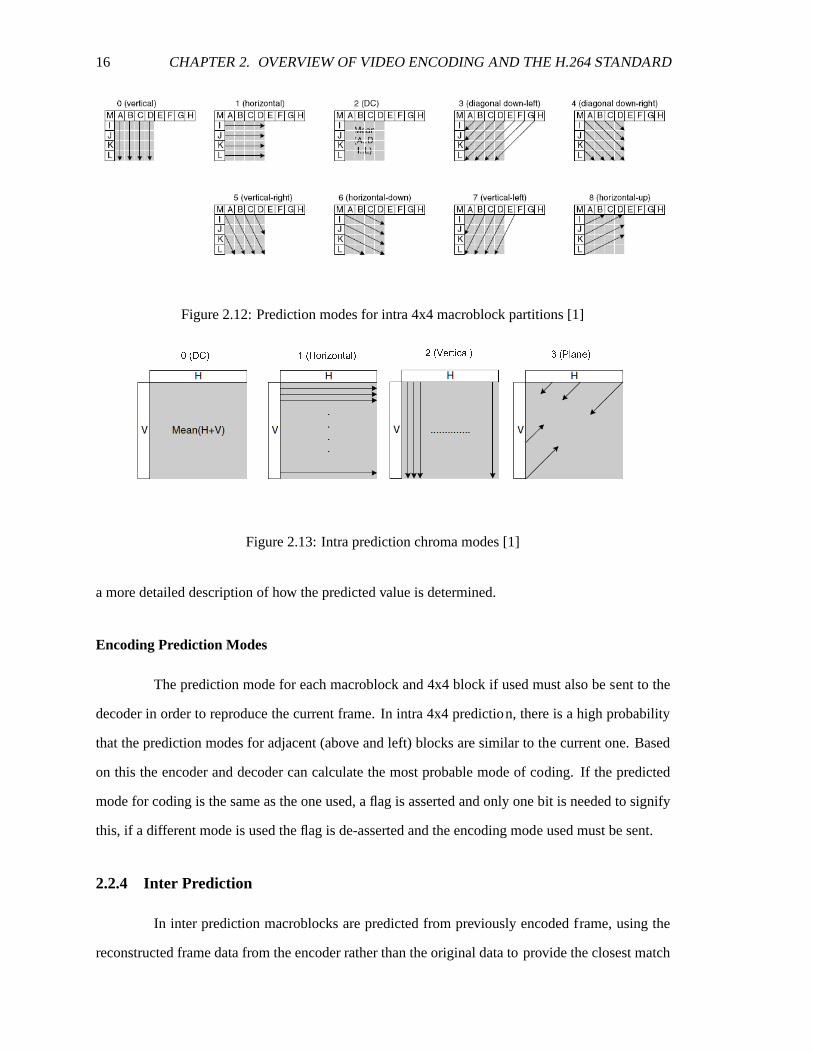
and within the same macroblock for the other 4x4 blocks. The modes available for prediction are
shown in Fig. 2.12. Vertical, horizontal, and DC modes are computed in a similar manner as intra
16x16 mode. For the remaining modes the predicted value is extrapolated fromthe top, left, and
top-right pixels. For a more detailed description of these modes please refer to the H.264 Standard.
Chroma Prediction
Intra chroma prediction is done independent of the luma prediction but with similar modes
to intra 16x16 prediction numbered differently. In DC prediction, the chromablock is divided into
a total of four 4x4 blocks and predicted in a similar manner to intra 4x4 blocks but with different
constraints on which side (H) or (V) is chosen for the prediction value. Please refer to standard for
16 CHAPTER 2. OVERVIEW OF VIDEO ENCODING AND THE H.264 STANDARD
Figure 2.12: Prediction modes for intra 4x4 macroblock partitions [1]0 ( D C ) 1 ( H o r i z o n t a l ) 2 ( V e r t i c a l ) 3 ( P l a n e )
Figure 2.13: Intra prediction chroma modes [1]
a more detailed description of how the predicted value is determined.
Encoding Prediction Modes
The prediction mode for each macroblock and 4x4 block if used must also be sent to the
decoder in order to reproduce the current frame. In intra 4x4 prediction, there is a high probability
that the prediction modes for adjacent (above and left) blocks are similar to the current one. Based
on this the encoder and decoder can calculate the most probable mode of coding. If the predicted
mode for coding is the same as the one used, a flag is asserted and only one bit is needed to signify
this, if a different mode is used the flag is de-asserted and the encoding mode used must be sent.
2.2.4 Inter Prediction
In inter prediction macroblocks are predicted from previously encoded frame, using the
reconstructed frame data from the encoder rather than the original data toprovide the closest match
2.2. OVERVIEW OF H.264 17
(a) ME Block Partition
(b) ME Sub-Block Partition
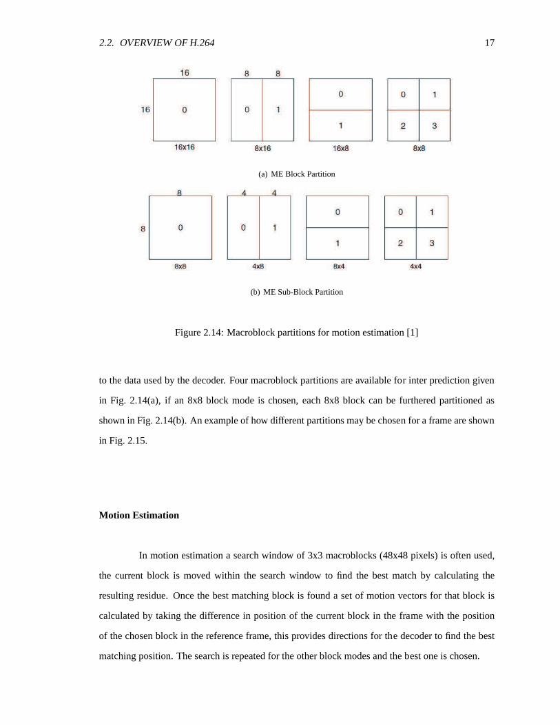
Figure 2.14: Macroblock partitions for motion estimation [1]
to the data used by the decoder. Four macroblock partitions are available for inter prediction given
in Fig. 2.14(a), if an 8x8 block mode is chosen, each 8x8 block can be furthered partitioned as
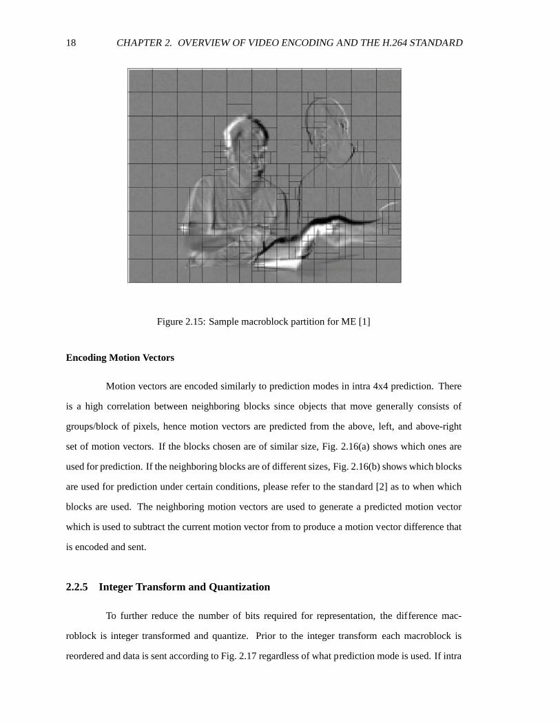
shown in Fig. 2.14(b). An example of how different partitions may be chosen for a frame are shown
in Fig. 2.15.
Motion Estimation
In motion estimation a search window of 3x3 macroblocks (48x48 pixels) is often used,
the current block is moved within the search window to find the best match by calculating the
resulting residue. Once the best matching block is found a set of motion vectors for that block is
calculated by taking the difference in position of the current block in the frame with the position
of the chosen block in the reference frame, this provides directions for the decoder to find the best
matching position. The search is repeated for the other block modes and the best one is chosen.
18 CHAPTER 2. OVERVIEW OF VIDEO ENCODING AND THE H.264 STANDARD
Figure 2.15: Sample macroblock partition for ME [1]
Encoding Motion Vectors
Motion vectors are encoded similarly to prediction modes in intra 4x4 prediction.There
is a high correlation between neighboring blocks since objects that move generally consists of
groups/block of pixels, hence motion vectors are predicted from the above, left, and above-right
set of motion vectors. If the blocks chosen are of similar size, Fig. 2.16(a)shows which ones are
used for prediction. If the neighboring blocks are of different sizes,Fig. 2.16(b) shows which blocks
are used for prediction under certain conditions, please refer to the standard [2] as to when which
blocks are used. The neighboring motion vectors are used to generate a predicted motion vector
which is used to subtract the current motion vector from to produce a motion vector difference that
is encoded and sent.
2.2.5 Integer Transform and Quantization
To further reduce the number of bits required for representation, the difference mac-
roblock is integer transformed and quantize. Prior to the integer transformeach macroblock is
reordered and data is sent according to Fig. 2.17 regardless of what prediction mode is used. If intra

2.2. OVERVIEW OF H.264 19
(a) ME Same Size Neighbor Blocks
(b) ME Different Size Neighbor Blocks
Figure 2.16: MV prediction from neighboring blocks [1]
20 CHAPTER 2. OVERVIEW OF VIDEO ENCODING AND THE H.264 STANDARD
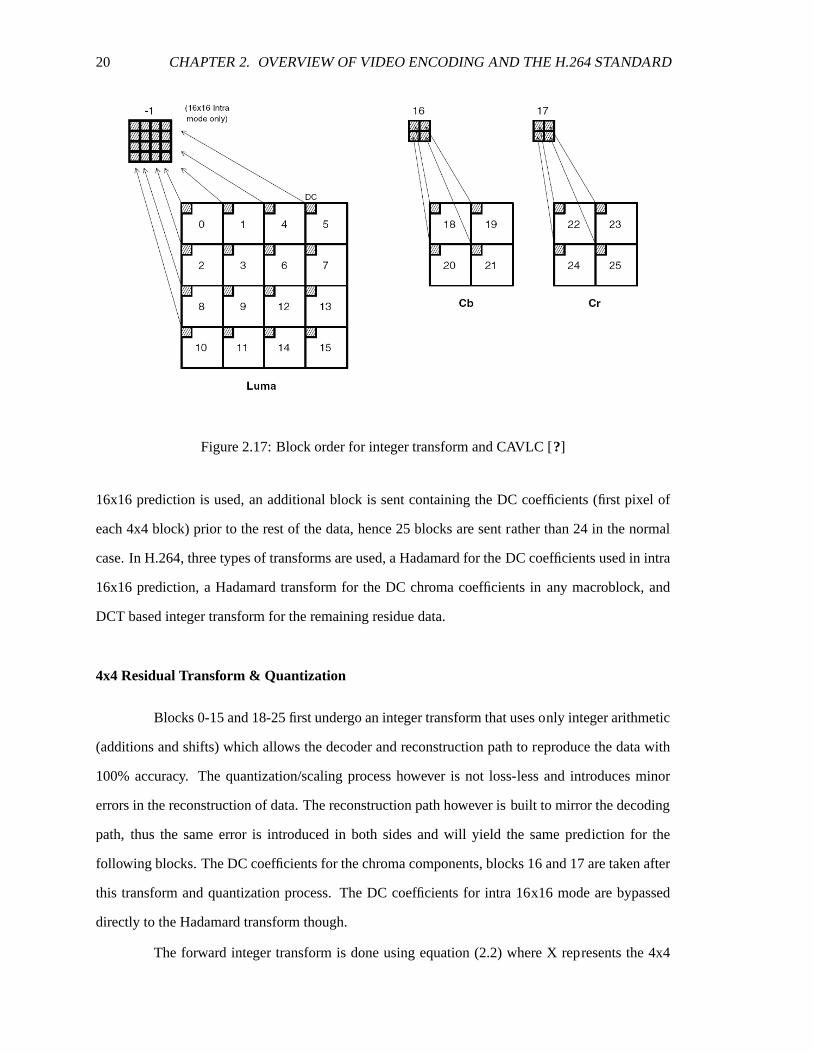
Figure 2.17: Block order for integer transform and CAVLC [?]
16x16 prediction is used, an additional block is sent containing the DC coefficients (first pixel of
each 4x4 block) prior to the rest of the data, hence 25 blocks are sent rather than 24 in the normal
case. In H.264, three types of transforms are used, a Hadamard for theDC coefficients used in intra
16x16 prediction, a Hadamard transform for the DC chroma coefficients inany macroblock, and
DCT based integer transform for the remaining residue data.
4x4 Residual Transform & Quantization
Blocks 0-15 and 18-25 first undergo an integer transform that uses only integer arithmetic
(additions and shifts) which allows the decoder and reconstruction path to reproduce the data with
100% accuracy. The quantization/scaling process however is not loss-less and introduces minor
errors in the reconstruction of data. The reconstruction path however isbuilt to mirror the decoding
path, thus the same error is introduced in both sides and will yield the same prediction for the
following blocks. The DC coefficients for the chroma components, blocks 16 and 17 are taken after
this transform and quantization process. The DC coefficients for intra 16x16 mode are bypassed
directly to the Hadamard transform though.
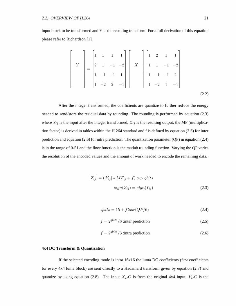
The forward integer transform is done using equation (2.2) where X represents the 4x4
2.2. OVERVIEW OF H.264 21
input block to be transformed and Y is the resulting transform. For a full derivation of this equation
please refer to Richardson [1].
Y
=
1 1 1 1
2 1 −1 −2
1 −1 −1 1
1 −2 2 −1
X
1 2 1 1
1 1 −1 −2
1 −1 −1 2
1 −2 1 −1
(2.2)
After the integer transformed, the coefficients are quantize to further reduce the energy
needed to send/store the residual data by rounding. The rounding is performed by equation (2.3)
whereYij is the input after the integer transformed,Zij is the resulting output, the MF (multiplica-
tion factor) is derived in tables within the H.264 standard and f is defined by equation (2.5) for inter
prediction and equation (2.6) for intra prediction. The quantization parameter (QP) in equation (2.4)
is in the range of 0-51 and the floor function is the matlab rounding function. Varying the QP varies
the resolution of the encoded values and the amount of work needed to encode the remaining data.
|Zij | = (|Yij | ∗ MFij + f) >> qbits
sign(Zij) = sign(Yij) (2.3)
qbits = 15 + floor(QP/6) (2.4)
f = 2qbits/6 :inter prediction (2.5)
f = 2qbits/3 :intra prediction (2.6)
4x4 DC Transform & Quantization
If the selected encoding mode is intra 16x16 the luma DC coefficients (first coefficients
for every 4x4 luma block) are sent directly to a Hadamard transform given by equation (2.7) and
quantize by using equation (2.8). The inputXDC is from the original 4x4 input,YDC is the
22 CHAPTER 2. OVERVIEW OF VIDEO ENCODING AND THE H.264 STANDARD
transformed output, andZDC is the quantize output. Qbits and f are defined as before andMF0,0
is the MF coefficient in the (0,0) position from the tables used in equation (2.3).
YDC
=
1 1 1 1
1 1 −1 −1
1 −1 −1 1
1 −1 1 −1
XDC
1 1 1 1
1 1 −1 −1
1 −1 −1 1
1 −1 1 −1
(2.7)
|ZDC(ij)| = (|YDC(ij)| ∗ MF0,0 + 2f) >> (qbits + 1)
sign(ZD(ij)) = sign(YD(ij)) (2.8)
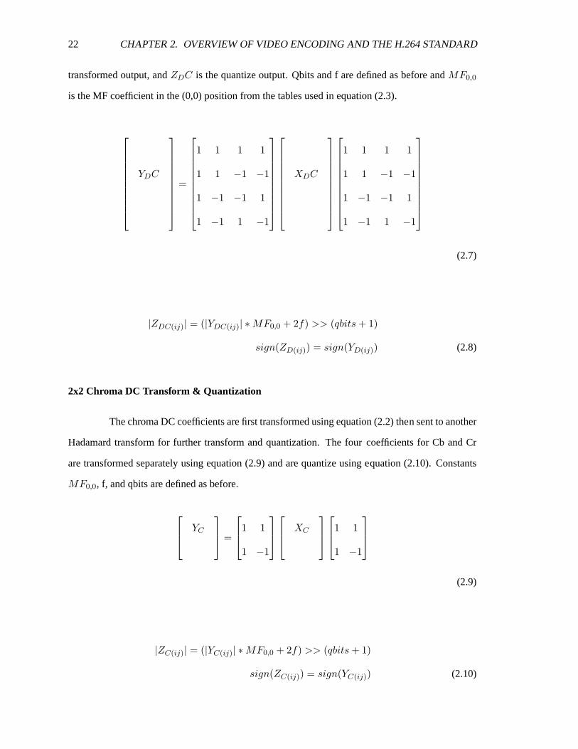
2x2 Chroma DC Transform & Quantization
The chroma DC coefficients are first transformed using equation (2.2) then sent to another
Hadamard transform for further transform and quantization. The fourcoefficients for Cb and Cr
are transformed separately using equation (2.9) and are quantize using equation (2.10). Constants
MF0,0, f, and qbits are defined as before.
YC
=
1 1
1 −1
XC
1 1
1 −1
(2.9)
|ZC(ij)| = (|YC(ij)| ∗ MF0,0 + 2f) >> (qbits + 1)
sign(ZC(ij)) = sign(YC(ij)) (2.10)
2.2. OVERVIEW OF H.264 23
2.2.6 Reference Frame Reconstruction
After the forward encoding process data is passed to both the entropy encoder and ref-
erence frame reconstruction block. The chroma DC coefficients and intra16x16 DC coefficients
are first inverse transformed and re-scaled then re-inserted back intotheir respective blocks before
being inverse transformed again. For details and the equations used for reconstruction please refer
to Richardson [1]. The reconstructed data is then stored and used for both intra and inter prediction.
2.2.7 Entropy Coding
After undergoing integer transform and quantization, the residue data can be further en-
coded using a context-adaptive variable-length coding method which takesadvantage that there are
mostly zeros, the number of non zero coefficients for neighboring blocksare correlated, most of the
non-zero data is either positive or negative one, and that coefficients closer to the DC value (closer
to the beginning) are generally higher. The prediction modes (intra prediction) and motion vectors
(inter prediction) however do not have these properties and are codedusing Exp-Golomb coding.
Exp-Golomb Coding
Exp-Golomb coding is used for encoding the prediction modes in intra prediction, motion
vectors in inter prediction and the block patterns for intra and inter prediction. The following ref-
erences tables are partially shown in this text, complete tables can be found in the H.264 standard
section 9.1.1. Intra and inter prediction modes are predicted using unsignedExp-Golomb codes in
Table 2.5. Motion vectors are first mapped to code numbers using Table 2.4 then the code words are
encoded using Table 2.6.
In encoding macroblocks, some blocks after the transform and quantization process con-
tain only data with value zero, these blocks do not need to be entropy encoded using the CAVLC but
can be signaled using the coded block pattern. The coded block pattern is a6-bit field with the first
four bits used to represent an 2x2 region of the macroblock (4 8x8 blocks). If all the data within that
block is zero then the corresponding bit is set to zero else it is set to one. The last two bits are used
to show the three possibilities for both chroma blocks this is shown in Table 2.7, once the codeNum
is obtained it is coded using Table 2.8 which correspond to the bit strings in Table 2.5.

24 CHAPTER 2. OVERVIEW OF VIDEO ENCODING AND THE H.264 STANDARD
codeNum syntax element value
0 0
1 1
2 -1
3 2
4 -2
... ...
Table 2.4: Signed ExpGolomb code table
Bit string codeNum inter mode
1 0 16x16
010 1 16x8
011 2 8x16
00100 3 8x8 w/ sub partition
00101 4 8x8 w/o sub partition
... ... ...
Table 2.5: Explicit Exp-Golomb code
Bit string form Range of codeNum
1 0
0 1X0 1-2
0 0 1X1 X0 3-6
0 0 0 1X2 X1 X0 7-14
... ...
Table 2.6: Prefix and suffix for codeNum
bit field description
5:4 00: All Chroma Data 0
01: DC = 0, AC != 0
10: DC 0, AC!= 0
3 0: Block = 0
2 1: Block != 0
1
0
Table 2.7: Coded block pattern for intra4x4 modes
2.2. OVERVIEW OF H.264 25
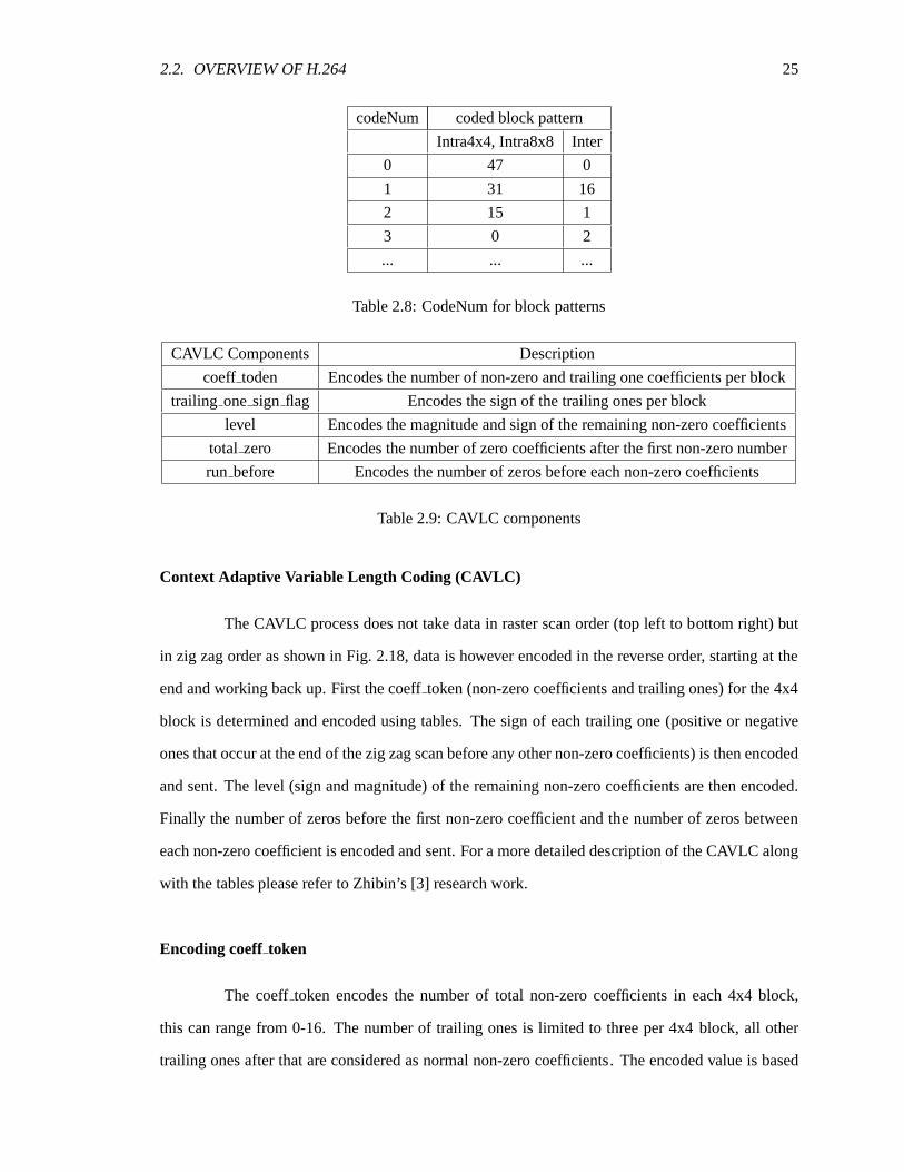
codeNum coded block pattern
Intra4x4, Intra8x8 Inter
0 47 0
1 31 16
2 15 1
3 0 2
... ... ...
Table 2.8: CodeNum for block patterns
CAVLC Components Description
coeff toden Encodes the number of non-zero and trailing one coefficients per block
trailing onesign flag Encodes the sign of the trailing ones per block
level Encodes the magnitude and sign of the remaining non-zero coefficients
total zero Encodes the number of zero coefficients after the first non-zero number
run before Encodes the number of zeros before each non-zero coefficients
Table 2.9: CAVLC components
Context Adaptive Variable Length Coding (CAVLC)
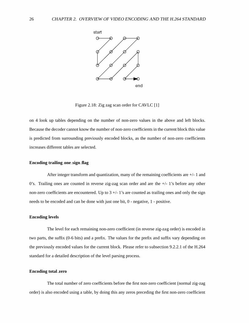
The CAVLC process does not take data in raster scan order (top left to bottom right) but
in zig zag order as shown in Fig. 2.18, data is however encoded in the reverse order, starting at the
end and working back up. First the coefftoken (non-zero coefficients and trailing ones) for the 4x4
block is determined and encoded using tables. The sign of each trailing one (positive or negative
ones that occur at the end of the zig zag scan before any other non-zero coefficients) is then encoded
and sent. The level (sign and magnitude) of the remaining non-zero coefficients are then encoded.
Finally the number of zeros before the first non-zero coefficient and the number of zeros between
each non-zero coefficient is encoded and sent. For a more detailed description of the CAVLC along
with the tables please refer to Zhibin’s [3] research work.
Encoding coeff token
The coefftoken encodes the number of total non-zero coefficients in each 4x4 block,
this can range from 0-16. The number of trailing ones is limited to three per 4x4block, all other
trailing ones after that are considered as normal non-zero coefficients. The encoded value is based
26 CHAPTER 2. OVERVIEW OF VIDEO ENCODING AND THE H.264 STANDARD
Figure 2.18: Zig zag scan order for CAVLC [1]
on 4 look up tables depending on the number of non-zero values in the above and left blocks.
Because the decoder cannot know the number of non-zero coefficients in the current block this value
is predicted from surrounding previously encoded blocks, as the number of non-zero coefficients
increases different tables are selected.
Encoding trailing one sign flag
After integer transform and quantization, many of the remaining coefficientsare +/- 1 and
0’s. Trailing ones are counted in reverse zig-zag scan order and arethe +/- 1’s before any other
non-zero coefficients are encountered. Up to 3 +/- 1’s are counted astrailing ones and only the sign
needs to be encoded and can be done with just one bit, 0 - negative, 1 - positive.
Encoding levels
The level for each remaining non-zero coefficient (in reverse zig-zag order) is encoded in
two parts, the suffix (0-6 bits) and a prefix. The values for the prefix and suffix vary depending on
the previously encoded values for the current block. Please refer to subsection 9.2.2.1 of the H.264
standard for a detailed description of the level parsing process.
Encoding total zero
The total number of zero coefficients before the first non-zero coefficient (normal zig-zag
order) is also encoded using a table, by doing this any zeros preceding the first non-zero coefficient
2.2. OVERVIEW OF H.264 27
NAL Unit Octet (bit) Description
7:3 NAL Unit Type
2:1 NAL Reference Id (NRI)
0 Forbidden Bit, always 0
Table 2.10: Bit field for NALU
will not need to be encoded.
Encoding run before
The number of zeros before each non-zero value is also encoded in order to reconstruct
the residual data block. Starting in reverse zig-zag scan order, the number of zeros is encoded. The
encoded value changes based on the number of zeros remaining and the last run of zeros before the
last coefficient does not need to be encoded since we already know thetotal number of zeros.
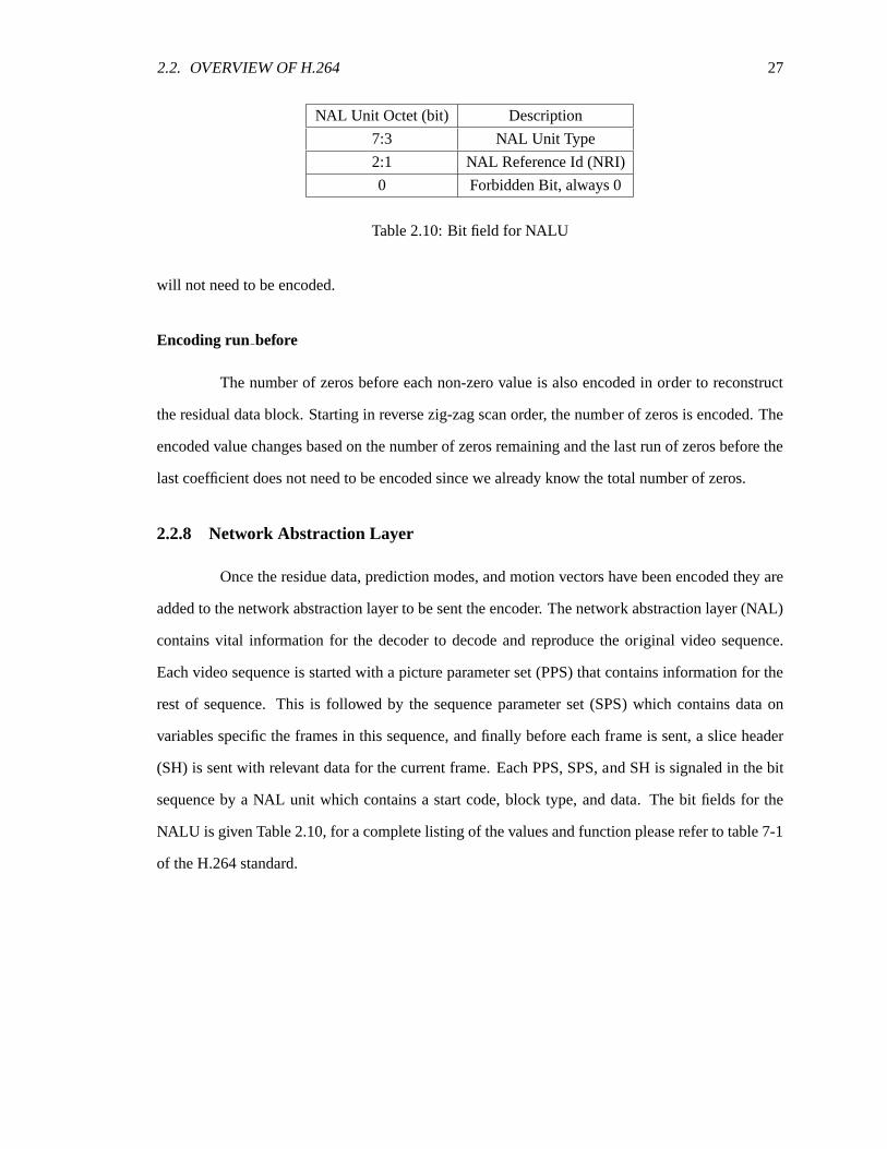
2.2.8 Network Abstraction Layer
Once the residue data, prediction modes, and motion vectors have been encoded they are
added to the network abstraction layer to be sent the encoder. The network abstraction layer (NAL)
contains vital information for the decoder to decode and reproduce the original video sequence.
Each video sequence is started with a picture parameter set (PPS) that contains information for the
rest of sequence. This is followed by the sequence parameter set (SPS) which contains data on
variables specific the frames in this sequence, and finally before each frame is sent, a slice header
(SH) is sent with relevant data for the current frame. Each PPS, SPS, and SH is signaled in the bit
sequence by a NAL unit which contains a start code, block type, and data. The bit fields for the
NALU is given Table 2.10, for a complete listing of the values and function please refer to table 7-1
of the H.264 standard.
28 CHAPTER 2. OVERVIEW OF VIDEO ENCODING AND THE H.264 STANDARD
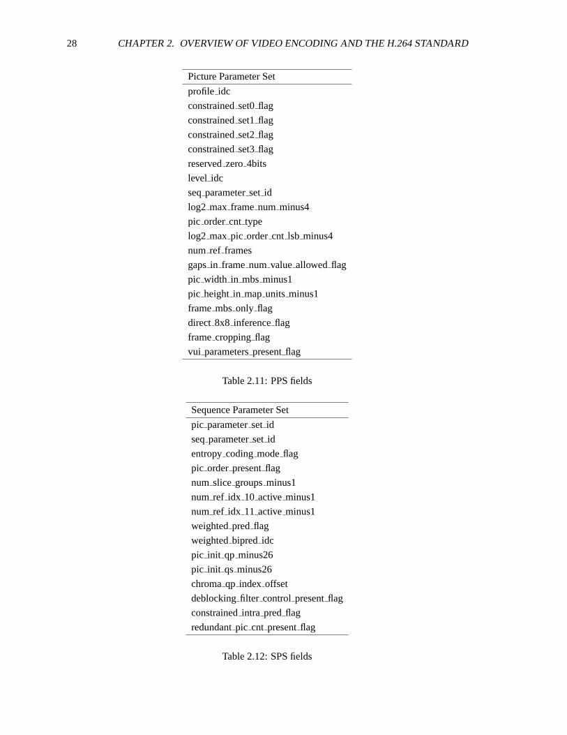
Picture Parameter Set
profile idc
constrainedset0flag
constrainedset1flag
constrainedset2flag
constrainedset3flag
reservedzero 4bits
level idc
seqparameterset id
log2 max frame num minus4
pic order cnt type
log2 max pic order cnt lsb minus4
num ref frames
gapsin frame num valueallowedflag
pic width in mbsminus1
pic height in mapunits minus1
frame mbsonly flag
direct 8x8 inferenceflag
frame croppingflag
vui parameterspresentflag
Table 2.11: PPS fields
Sequence Parameter Set
pic parameterset id
seqparameterset id
entropycodingmodeflag
pic order presentflag
num slice groupsminus1
num ref idx 10 activeminus1
num ref idx 11 activeminus1
weightedpred flag
weightedbipred idc
pic init qp minus26
pic init qs minus26
chromaqp index offset
deblockingfilter control presentflag
constrainedintra pred flag
redundantpic cnt presentflag
Table 2.12: SPS fields

2.2. OVERVIEW OF H.264 29
Slice Header
first mb in slice
slice type
pic parameterset id
frame num
idr pic id
pic order cnt lsb
no outputof prior flag
long term referenceflag
slice qp delta
Table 2.13: SH fields

30 CHAPTER 2. OVERVIEW OF VIDEO ENCODING AND THE H.264 STANDARD
31
Chapter 3
Processing Platforms Used for Video
Encoding
Various platforms have been used for video processing with varying results. The platform
spectrum ranges from general purpose computers to chips built specifically for video encoding,
depending on the application performance needed, different platforms are chosen. This chapter
looks at some the various platforms used for video encoding and presentsthe proposed platform.
3.1 Related Work in H.264 Processing
Previous implementations of H.264 video encoders have been done on nearly all levels.
Encoders on general purpose (GP) processors have been developed as the golden model for compar-
ison and development. General purpose processors however are not able to meet the constraints of
real-time video encoding and is used primarily as a reference point. Multimedia co-processors have
also been used for video encoding, these however have focused on smaller frame sizes, generally
CIF and below with high power consumptions making them not as desirable in portable applications.
ASIC have managed to provide low power real time video encoding, however since these processors
are application specific, they cannot be easily modified for future implementations or other config-
urations. Section 3.1.1 presents implementations on GP processors, section 3.1.2 presents solution
on DSP chips, and section 3.1.3 presents ASIC implementations.

32 CHAPTER 3. PROCESSING PLATFORMS USED FOR VIDEO ENCODING
GP Processing Platform
Processor Type Intel Xeon w/ HT
Number of Processors4
Threads 8
Speed 2.8GHz
L2 Cache 256 KB
L3 Cache 2 MB
Performance 4.6 frames/s (CIF)
Table 3.1: Performance of H.264 Video encoder on Intel Quad Core Processor [4]
DSP Processing Platform
Processor Intel PXA27x
Speed 624 MHz
Accelerator Intel MMX (64-bit SIMD)
Memory
Performance 49 frames/s (QCIF Average)
Table 3.2: Performance of video encoder on Intel DSP platform [5]
3.1.1 Video Encoding on General Purpose (GP) Processors
The H.264 video encoder is implemented in software for general purpose processors,
Chen and others [4] looks specifically at optimizing an encoder on Intel’s Pentium 4 processor.
Because of the complexity of the encoding process their implementation was done using proces-
sors with multi-threading capabilities using software optimization to speed up the process by 4.6x
over traditional SIMD implementations which provide approximately 1 frame/s forCIF-resolution
sequences.
3.1.2 Video Encoding on Digital Signal Processors (DSP)
Digital signal processors have provided more promising results with fasterthroughput.
Wei and others [5] has implemented a real time H.264 video encoder on an Intel PXA27x processor
used on the HP IPAQ hx4700 PDA which includes Intel’s Wireless MMX technology for multimedia
acceleration yielding an average of 49 frames/s for CIF-resolution sequences using a QP value of
28.
3.2. PROPOSED H.264 VIDEO ENCODER PLATFORM 33
ASIC Processing Platform
Technology .180 um CMOS
Voltage 1.8V
Core Area 7.68 x 4.13 mm2
SRAM 34.72 KB
Performance 81 MHz
(SD 720x480) 581 mW
Performance 108 MHz
(720p 1280x720) 785 mW
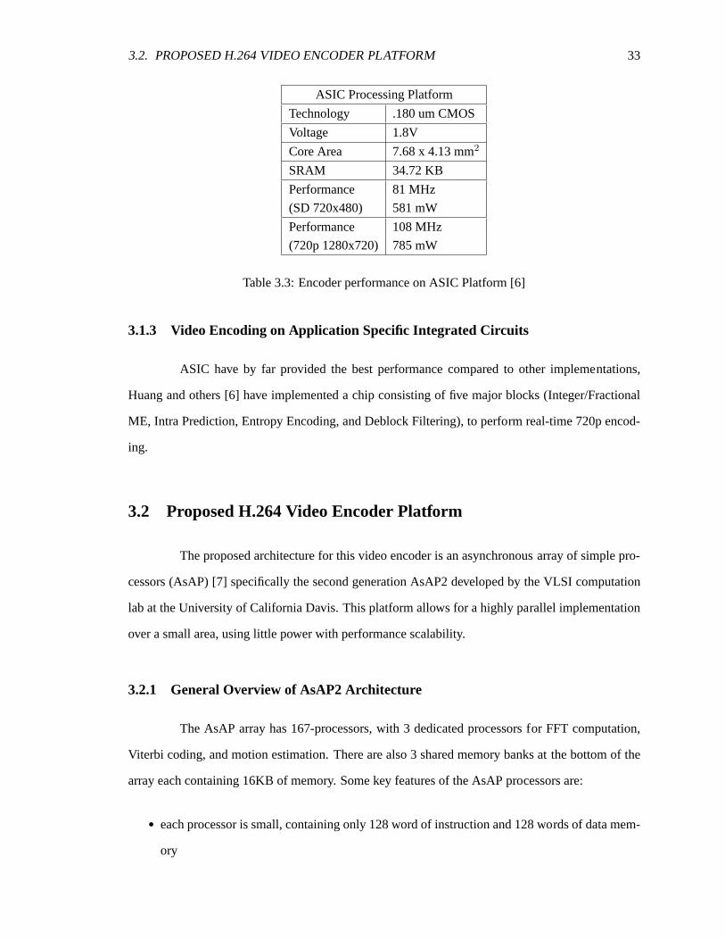
Table 3.3: Encoder performance on ASIC Platform [6]
3.1.3 Video Encoding on Application Specific Integrated Circuits
ASIC have by far provided the best performance compared to other implementations,
Huang and others [6] have implemented a chip consisting of five major blocks (Integer/Fractional
ME, Intra Prediction, Entropy Encoding, and Deblock Filtering), to perform real-time 720p encod-
ing.
3.2 Proposed H.264 Video Encoder Platform
The proposed architecture for this video encoder is an asynchronousarray of simple pro-
cessors (AsAP) [7] specifically the second generation AsAP2 developed by the VLSI computation
lab at the University of California Davis. This platform allows for a highly parallel implementation
over a small area, using little power with performance scalability.
3.2.1 General Overview of AsAP2 Architecture
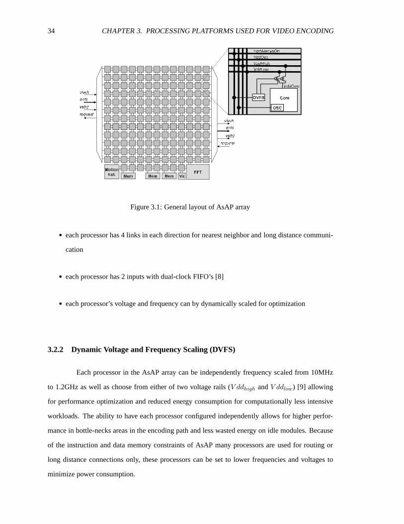
The AsAP array has 167-processors, with 3 dedicated processors for FFT computation,
Viterbi coding, and motion estimation. There are also 3 shared memory banks atthe bottom of the
array each containing 16KB of memory. Some key features of the AsAP processors are:
• each processor is small, containing only 128 word of instruction and 128 words of data mem-
ory
34 CHAPTER 3. PROCESSING PLATFORMS USED FOR VIDEO ENCODING
M e m V i tM o t i o nE s t . M e m M e md a t ar e q u e s t
V d d H i g hV d d L o wV d d A l w a y s O nV d d O s cD V F S O S C V d d C o r ec l o c kv a l i d d a t ar e q u e s tc l o c kv a l i d
F F TC o r e
Figure 3.1: General layout of AsAP array
• each processor has 4 links in each direction for nearest neighbor andlong distance communi-
cation
• each processor has 2 inputs with dual-clock FIFO’s [8]
• each processor’s voltage and frequency can by dynamically scaled for optimization
3.2.2 Dynamic Voltage and Frequency Scaling (DVFS)
Each processor in the AsAP array can be independently frequency scaled from 10MHz
to 1.2GHz as well as choose from either of two voltage rails (V ddhigh andV ddlow) [9] allowing
for performance optimization and reduced energy consumption for computationally less intensive
workloads. The ability to have each processor configured independently allows for higher perfor-
mance in bottle-necks areas in the encoding path and less wasted energy onidle modules. Because
of the instruction and data memory constraints of AsAP many processors areused for routing or
long distance connections only, these processors can be set to lower frequencies and voltages to
minimize power consumption.
3.2. PROPOSED H.264 VIDEO ENCODER PLATFORM 35
Frequency Voltage Power
1.2 GHz 1.3 V 62 mW
1.07 GHz 1.2 V 47.5 mW
66 MHz .675 V .608 mW
Table 3.4: AsAP power measurements for various voltage and frequencyconfigurations
3.2.3 Memory Architecture
Each processor has 128 words of instruction memory for programming and128 word data
memory for storage, a 27 word dynamic configuration memory is also available for use as pointers
and setting input output configurations. The data memory (DMem) is a single ported SRAM 16-bits
wide by 128 words. The memory space is replicated allowing for memory access for two operands
in a single cycle. The three shared memory (16 KB each) [10] at the bottom of the processor array
can be accessed by two processor each for additional storage space. Each contains a single ported
16-bit x 8KWord SRAM with single cycle read and writes.
3.2.4 Processor Interconnect
Each processor has 8 links as shown in Figure 3.2, the links are independent of the core
so they can configured for long distance communication (bypassing the core). Two dual clock
FIFOs can connect any of the 8 links to the core for input data. The dualclock FIFO’s allow
each core to run at a separate frequency and still be able to communicate witheach other. Each
FIFO is 64 words deep with a stall signal to tell the communicating processor when it is full.
The link directions are signified by north, east, south, west, and up, down, left, right. For long
distance communication, compass direction outputs can talk to any other compassdirection, and
any direction output can be connected to another (north and connect to south but not down). The
input direction to each processor is statically configured during programming, while the output
direction can by dynamically switched during run-time.
3.2.5 Motion Estimation Accelerator
Motion estimation is a highly computational task and has been implemented as a hardware
processor on AsAP. The motion estimation accelerator (MEACC) [11] allows for communication

36 CHAPTER 3. PROCESSING PLATFORMS USED FOR VIDEO ENCODING
Figure 3.2: Major blocks in AsAP processor
Processor Processor
East In
East Out
Right Out
Right In
Sou
th O
ut
South
In
Do
wn
Ou
t
Do
wn
In
West Out
West In
Left out
Left In
No
rth
In
Nort
h O
ut
Up
In
Up
Ou
t
Figure 3.3: Nearest neighbor communication links for AsAP processors
3.2. PROPOSED H.264 VIDEO ENCODER PLATFORM 37
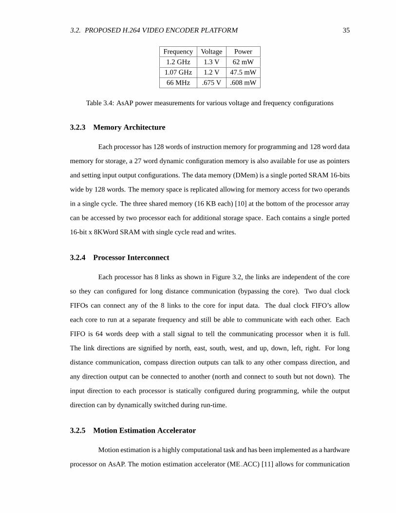
Figure 3.4: block diagram ME accelerator on AsAP2
with two neighboring processors for control. The block diagram for the ME ACC is given in Fig-
ure 3.4. The accelerator has its own memory for storing the current macroblock and search window
allowing for faster computation.
General Architecture
After the ME ACC loads the required current and reference data, a set of searchpatterns
is loaded along with the block size used for prediction and the start signal. The ME ACC will then
return the SAD value for that search position to the neighboring processor, this can be continued by
sending a continue signal or abort signal once the neighboring processor determines that a sufficient
match has been found.
Dedicated Memory
The ME ACC has two dedicated memory banks one for storing the current macroblock
and one for storing the reference search window. The current macroblock memory consist of 2
banks, each 8 8-bit words wide, and with 16 rows, allowing for one 16x16 macroblock. The refer-

38 CHAPTER 3. PROCESSING PLATFORMS USED FOR VIDEO ENCODING
Figure 3.5: Steps for running ME accelerator
ence memory contains 8 banks each 8 8-bit words wide with 64 rows allowing for 16 macroblocks
(4x4 macroblocks). The extra row and column in the reference memory canbe used for pre-loading
of memory to hide latency. For a more detailed description of the memory architecture please refer
to Gouri’s thesis [11].
Programmable Search Algorithm
The search area and pattern in the MEACC are user defined allowing for different types of
searches such as full search, 4-step, diamond as well as any custom ones. The accelerator currently
allows for 4 sets of search patterns, each with 64 different programmablesearch locations. During
run time the desired search pattern is selected by writing to a register, the indexes in the search
pattern are then incremented by writing to the MECONT register.
3.2. PROPOSED H.264 VIDEO ENCODER PLATFORM 39
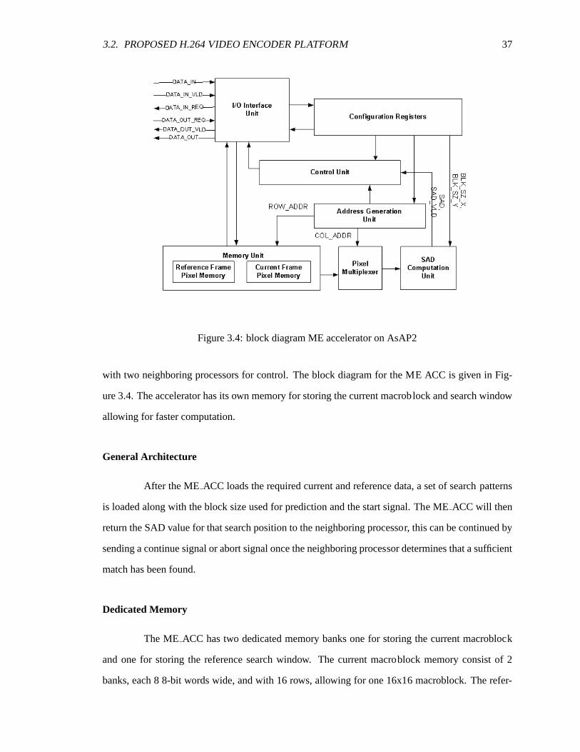
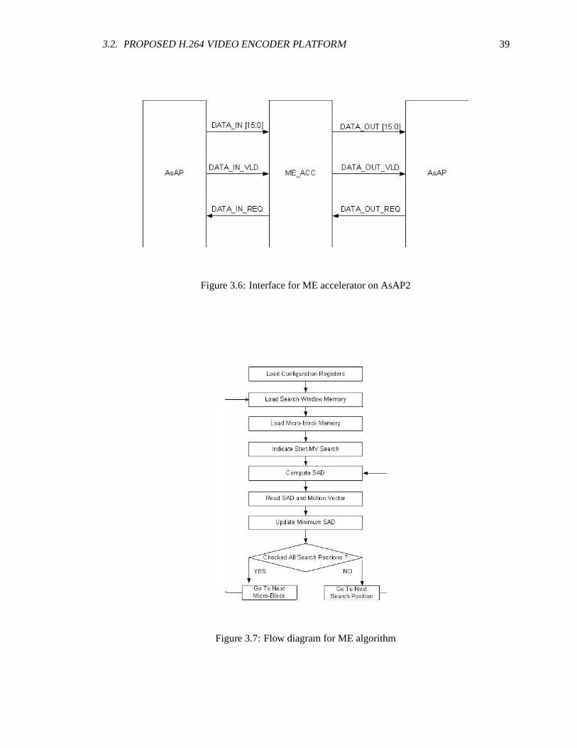
Figure 3.6: Interface for ME accelerator on AsAP2
Figure 3.7: Flow diagram for ME algorithm

40 CHAPTER 3. PROCESSING PLATFORMS USED FOR VIDEO ENCODING
41
Chapter 4
Parallel Programming Tools
A high level C H.264 video encoder was first developed as a referencemodel for the
AsAP implementation using the message passing interface (MPI). Due to the complexity of parallel
programming a MPI wrapper was used and is discussed in the following section. The next section
deals with issues in converting the MPI/C program to assembly for AsAP.
4.1 Message Passing Interface (MPI)
The message passing interface is a specification for an application programming interface
(API) allowing multiple computers to commute with each other while running a single program.
However, programming with the MPI syntax can be confusing and time consuming since many of
the commands required are simply for communication protocols. Two tools have been developed by
Paul and Eric [12] to make this process easier. The first is a MPI wrapper allowing the programmer
to essentially use C, and the second is a mapping tool for a visual connectionof parallel programs.
4.1.1 Parallel C/MPI Wrapper
The MPI wrapper allows the programmer to write in C with a few key words for desig-
nating different nodes such as begin, end, ibuf, and obuf. Once the Ccode is written a script goes
through and add the necessary instruction for making the code compatible for an MPI simulator.
42 CHAPTER 4. PARALLEL PROGRAMMING TOOLS
4.1.2 AsAP Arbitrary Mapping Tool
The arbitrary mapping tool allows the programmer to visually see the connections for each
parallel program block and connect them making the communication between blocks easier. The
tool also follows the AsAP model and can propose a mapping algorithm for mapping the programs
onto an AsAP chip. Here since the programs are written in C and not assembly, the primary use of
the tool was for a visual mapping of the C blocks.
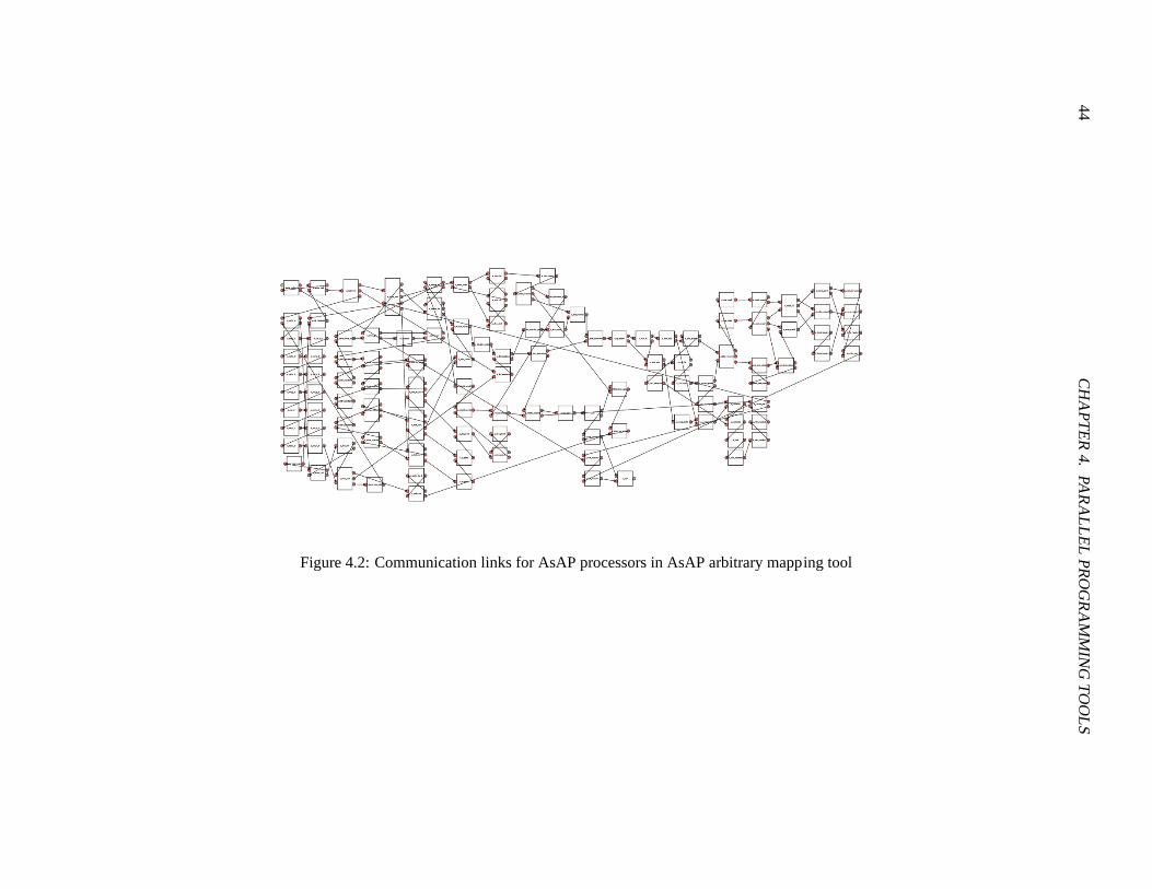
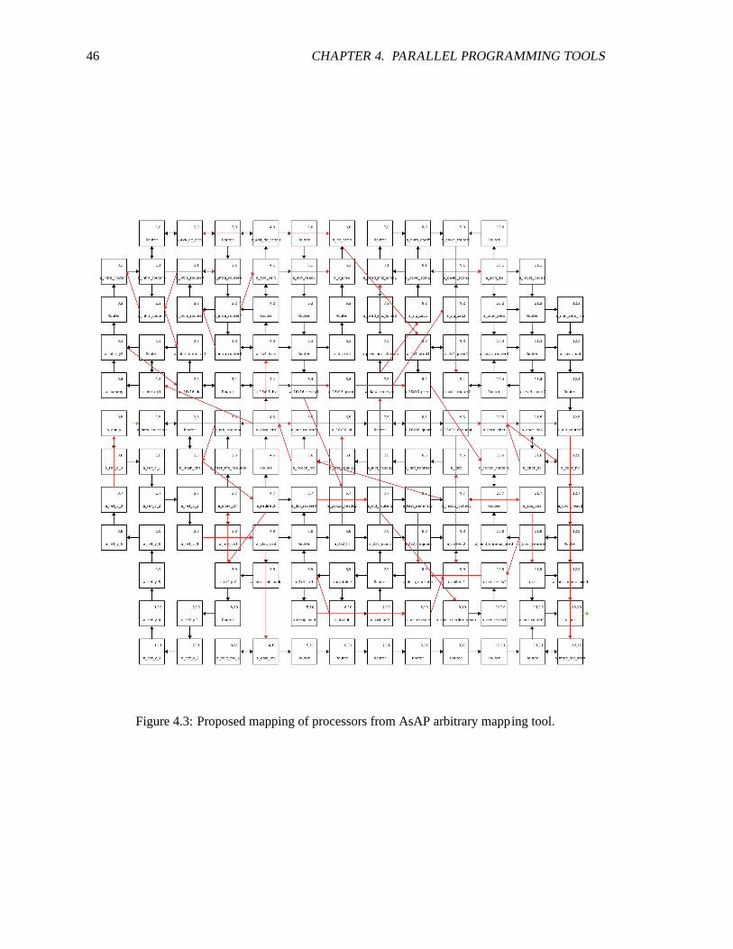
Figure 4.1 shows the encoder modules in C and Fig. 4.2 shows the low level processors
that model those same processors in AsAP assembly. An example mapping of these processors to
the AsAP chip is shown in Fig. 4.3, in this implementation however a hand mapping is used for
simplicity. Because the encoder is programmed in parts, using the mapping tool, every time a new
processors is added, would require the programmer to go back and and change all the processor
coordinates by hand. A comparison of the hand mapped encoder to the proposed mapping from the
tool is given in the analysis section.

4.1.M
ES
SA
GE
PA
SS
ING
INT
ER
FAC
E(M
PI)
43
Figure 4.1: Communication links for reference C model in AsAP arbitrary mapping tool
44C
HA
PT
ER
4.P
AR
ALLE
LP
RO
GR
AM
MIN
GT
OO
LS
Figure 4.2: Communication links for AsAP processors in AsAP arbitrary mapping tool
4.2. PARALLEL PROGRAMMING 45
4.2 Parallel Programming
Because programming on AsAP is considerably different than C or traditional assembly
this section talks about the methodologies used in programming, what had to be changed and altered,
what was harder, what was improved, and what are some of the common problems/pitfalls that were
encountered in programming this video encoder.
4.2.1 Methodology
Two main differences in programming AsAP vs. other chips or using MPI is thesize of
the instruction/data memory available and the input limits per processor.
Limited Data Memory - Processors
Video encoding is a highly memory intensive process, from the sheer size of throughput
needed for standard quality video to the memory reference needed for prediction, the 128 data
memory posed as a great challenge. Because there is only 128 16-bit words of memory, even
if the macro block data is packed, it would not fit onto a single processor and would have to be
split into at least two, with the luma data packed (two pixels per word) into one processor and the
chroma data into another processor. Even so that leaves no memory left in the luma processors for
variables using in calculations, hence the memory processors would have tobe separate from the
computational processors. Data is accessed by using the dynamic configuration memory (DCMem)
to determine where in the processor the data resides and passes it along. When more data space is
needed (but significantly less than that provided by the big memories) multiple processors can be
connected in a loop to form a FIFO like buffer.
Limited Instruction Memory
The small instruction memory available for each processor is fairly adequatefor simple
tasks, however to perform more computationally intensive task, the programs had to be split up into
smaller blocks. This creates more parallelism if the program can be broken up in such a manner
that both blocks can be executed at the same time. The challenge is to find goodbreaking points in
the program where branching off to another processor would requirelittle overhead because certain
46 CHAPTER 4. PARALLEL PROGRAMMING TOOLS
Figure 4.3: Proposed mapping of processors from AsAP arbitrary mapping tool.

4.2. PARALLEL PROGRAMMING 47
control information and data would be needed by both/multiple processors. Generally it is safe to go
to a different processor once you have exited all conditional loops including if statements because
there would generally be less data overlap and only a few control values need to be passed along
with what was recently computed.
Limited Inputs
Perhaps the biggest difference in programming in AsAP is the limited number of inputs
to both the chip and each individual processors. The AsAP2 chip has only one external input and
output for off chip communication thus not suitable to control flow operationswhere the input
depends on the output. Because of the limited memory on board the current and reference frames
cannot be stored on chip and must be stored off chip in the FPGA, when a processor needed a
macroblock, it would send a request signal. Since there is only one output,the request signal and
encoded video output must both share this, requiring that control bits be sent to the FPGA for
determining where each output should be routed.
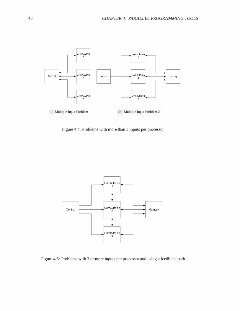
Having only two inputs per processor core posed an even greater challenge. Because of
the limited instruction memory, many of the modules had to be broken up to smaller parts, and at
some later point combined again to re-construct the data as shown in Fig. 4.4(a). A similar problem
is where each processor now also requires inputs from multiple sources as shown in Fig. 4.4(b). The
biggest challenge however is when there is data and control dependencies between the processors
as shown in Fig. 4.5, each processor not only needs to communicate with the control and memory
processors, but also pass along data amongst themselves.
In general, three different solutions were used depending which problem type was en-
countered and what conditions/constraints were needed. For problem 1the solution in Fig. 4.6(a)
is simple and sufficient, using additional processors for routing, adding the inputs together two at a
time until all of them could be combines, similar to building a multiple input AND gate fromonly
two input AND gates. The only constraint is that the data flow must be know, which input would
data appear at first and how many data points should be taken from each input to ensure proper
data flow. Solution 2 can also be used to solve either problem 1, 2, and 3. However for solving
problem 3, this method requires all the above processors to stall while waitingfor data to return for
the requesting processor below it. Interrupts cannot be used since there are only two inputs so it
48 CHAPTER 4. PARALLEL PROGRAMMING TOOLS
C o n t r o lC o m p u t a t i o n1C o m p u t a t i o n2C o m p u t a t i o n3
(a) Multiple Input Problem 1
C o n t r o l M e m o r yC o m p u t a t i o n1C o m p u t a t i o n2C o m p u t a t i o n3
(b) Multiple Input Problem 2
Figure 4.4: Problems with more than 3 inputs per processor
C o n t r o l M e m o r yC o m p u t a t i o n1C o m p u t a t i o n2C o m p u t a t i o n3
Figure 4.5: Problems with 3 or more inputs per processor and using a feedback path

4.2. PARALLEL PROGRAMMING 49
cannot be determined if the data was requested by the current processor or one below it. Adding in
the extra word for control is possible, but now generates the problem ofextra instructions used for
checking the condition every time a new data is received. Since AsAP does not support traditional
interrupts, branch on empty FIFO conditions are used to avoid stalling. These branch instructions
must be added often throughout the program to avoid stalling other processors, this would however
require additional instruction memory which is not readily available. Solution 2 ismost useful when
a program is split between multiple processors and one must stall while waiting for data to be com-
puted by another processor that requires additional data that cannot be stored locally. An example
is when computing SAD values and the current macroblock data is stored on another processors.
The third solution provides a method for avoiding the latency of solution 2 but requires
3 times the number of processors. In Fig. 4.7 the data path up the computationalprocessor are for
passing control information along as well as conditions or complete signals. Routers 1-3 are used
for sending request for data, router 1 is the problem, requiring 3 additional routers. Since router 1
already has two inputs from the requesting processor it cannot also receive data from the memory
processor, thus requiring routers 4-6 to send back the requested data. Routers 4-6 can also be used to
passing information from computational processors 1, 2, and 3 becausedirect links are not available
as in solution 2. Since it is not known when a processor might request data, tags are also assigned
to requested data to determine which processor was the original requester.
4.2.2 Pitfalls
The bulk of debugging time in programming AsAP has been centered around several key
issues that were discussed above, primarily the program splitting and processor intercommunication.
I/O Mis-Match
Because of sheer size of the program, making sure that data is processed in the proper
order has been extremely difficult. The main processing block in video encoding is the 16x16 mac-
roblock, when data is passed between modules they must generally be senttogether, and must all
be present before continuing, however because each macroblock contains 384 words they cannot
be stored on any single processor, to reduce the number of processors used for simply storing data,

50 CHAPTER 4. PARALLEL PROGRAMMING TOOLS
C o n t r o l C o m p u t a t i o n1C o m p u t a t i o n2C o m p u t a t i o n3
R o u t e r
(a) Multiple input solution 1
C o n t r o lM e m o r y C o m p u t a t i o n1
C o m p u t a t i o n2C o m p u t a t i o n3
(b) Multiple input solution 2
Figure 4.6: Solutions for more than 2 inputs per processorC o n t r o lM e m o r y C o m p u t a t i o n1
C o m p u t a t i o n2C o m p u t a t i o n3
R o u t e r 1R o u t e r 2R o u t e r 3
R o u t e r 4R o u t e r 5R o u t e r 6
Figure 4.7: Solution for 3 or more inputs per processor with feedback
4.2. PARALLEL PROGRAMMING 51
when data is to be compared such as in comparing SADs for different modes, the comparing pro-
cessor must wait for all other to complete before continuing, this may cause some processors to stall
in the process. To ensure that data is passed along correctly the simplest methods are often used
rather than the most efficient algorithms.
Program Splitting Overhead
As mentioned above splitting programs to blocks that would fit inside each processor
requires a certain amount of overhead. It is often tempting to try and optimize the code and try to fit
it to exactly 128 words, this however leaves no room for changes or improvements. If anything needs
to be altered, the entire code must be re-written. The simplest solution is often better, breaking up
the program while requiring additional overhead and added complexity to processor communication
allows for the most room for further improvements and additions and program scalability
Error Tracing
Error tracing in AsAP has proved to be rather difficult, because it is not often possible to
tell directly which processor is causing the problem. Errors were generally due to I/O mismatches
rather than computational problems. To solve this the program counter must be looked at for each
processor then matched to the instruction to determine the trace-back path forthe error.

52 CHAPTER 4. PARALLEL PROGRAMMING TOOLS

53
Chapter 5
Implementation
Because of the complexity of video encoding and the H.264 standard, not all aspects of
the standard are implemented in this work. Some key differences from the standard that are not
implemented in both the C model and AsAP version are sub-pixel interpolation in inter prediction,
inter prediction is limited to 1 reference frame, intra prediction is limited to 3 modes only, and
no de-block filtering is implemented. Using a programmable platform however allows for these
additional function to be added at a later time. This chapter goes into more detailof the MPI model
and AsAP implementation.
5.1 Parallel C Implementation
The parallel C implementation was developed following the guidelines from the standard
[2] and the reference software JM version 12.1. In the C programs, code is kept as simple as
possible using only standard functions and basic data elements such as integers and arrays for an
easy transition to assembly. Since there are no memory constraints in C, all current/reference frame
data is stored locally. The .h264 bitstream output of this implementation is compatible with the
reference JM decoder software and can be viewed on third party YUV viewing software.
5.1.1 General Overview
The main difference between the MPI model and the standard encoder shown in Chapter 2
is that there is no de-block filtering. Because this version is used as a reference model for developing
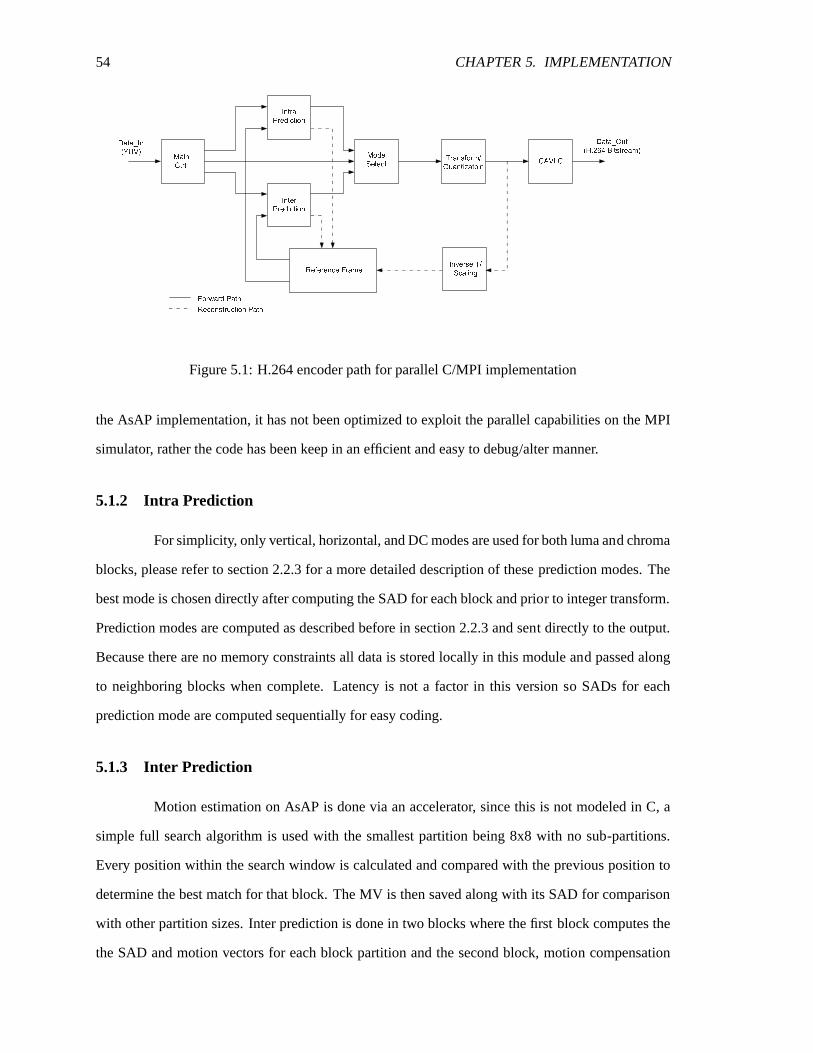
54 CHAPTER 5. IMPLEMENTATION
M a i nC t r l . I n t r aP r e d i c t i o nI n t e rP r e d i c t i o n M o d eS e l e c t T r a n s f o r m /Q u a n t i z a t o i n
I n v e r s e T /S c a l i n gC A V L C
R e f e r e n c e F r a m eF o r w a r d P a t hR e c o n s t r u c t i o n P a t hD a t a _ I n( Y U V ) D a t a _ O u t( H . 2 6 4 B i t s t r e a m )
Figure 5.1: H.264 encoder path for parallel C/MPI implementation
the AsAP implementation, it has not been optimized to exploit the parallel capabilitieson the MPI
simulator, rather the code has been keep in an efficient and easy to debug/alter manner.
5.1.2 Intra Prediction
For simplicity, only vertical, horizontal, and DC modes are used for both luma and chroma
blocks, please refer to section 2.2.3 for a more detailed description of theseprediction modes. The
best mode is chosen directly after computing the SAD for each block and prior to integer transform.
Prediction modes are computed as described before in section 2.2.3 and sent directly to the output.
Because there are no memory constraints all data is stored locally in this module and passed along
to neighboring blocks when complete. Latency is not a factor in this version so SADs for each
prediction mode are computed sequentially for easy coding.
5.1.3 Inter Prediction
Motion estimation on AsAP is done via an accelerator, since this is not modeled in C, a
simple full search algorithm is used with the smallest partition being 8x8 with no sub-partitions.
Every position within the search window is calculated and compared with the previous position to
determine the best match for that block. The MV is then saved along with its SAD for comparison
with other partition sizes. Inter prediction is done in two blocks where the firstblock computes the
the SAD and motion vectors for each block partition and the second block, motion compensation
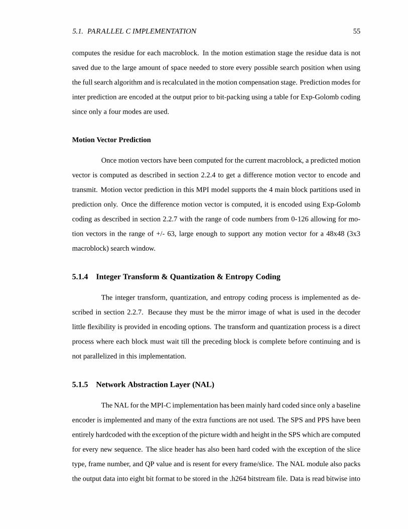
5.1. PARALLEL C IMPLEMENTATION 55
computes the residue for each macroblock. In the motion estimation stage the residue data is not
saved due to the large amount of space needed to store every possible search position when using
the full search algorithm and is recalculated in the motion compensation stage. Prediction modes for
inter prediction are encoded at the output prior to bit-packing using a table for Exp-Golomb coding
since only a four modes are used.
Motion Vector Prediction
Once motion vectors have been computed for the current macroblock, a predicted motion
vector is computed as described in section 2.2.4 to get a difference motion vector to encode and
transmit. Motion vector prediction in this MPI model supports the 4 main block partitions used in
prediction only. Once the difference motion vector is computed, it is encodedusing Exp-Golomb
coding as described in section 2.2.7 with the range of code numbers from 0-126 allowing for mo-
tion vectors in the range of +/- 63, large enough to support any motion vectorfor a 48x48 (3x3
macroblock) search window.
5.1.4 Integer Transform & Quantization & Entropy Coding
The integer transform, quantization, and entropy coding process is implemented as de-
scribed in section 2.2.7. Because they must be the mirror image of what is usedin the decoder
little flexibility is provided in encoding options. The transform and quantization process is a direct
process where each block must wait till the preceding block is complete before continuing and is
not parallelized in this implementation.
5.1.5 Network Abstraction Layer (NAL)
The NAL for the MPI-C implementation has been mainly hard coded since only a baseline
encoder is implemented and many of the extra functions are not used. The SPS and PPS have been
entirely hardcoded with the exception of the picture width and height in the SPSwhich are computed
for every new sequence. The slice header has also been hard codedwith the exception of the slice
type, frame number, and QP value and is resent for every frame/slice. The NAL module also packs
the output data into eight bit format to be stored in the .h264 bitstream file. Data isread bitwise into
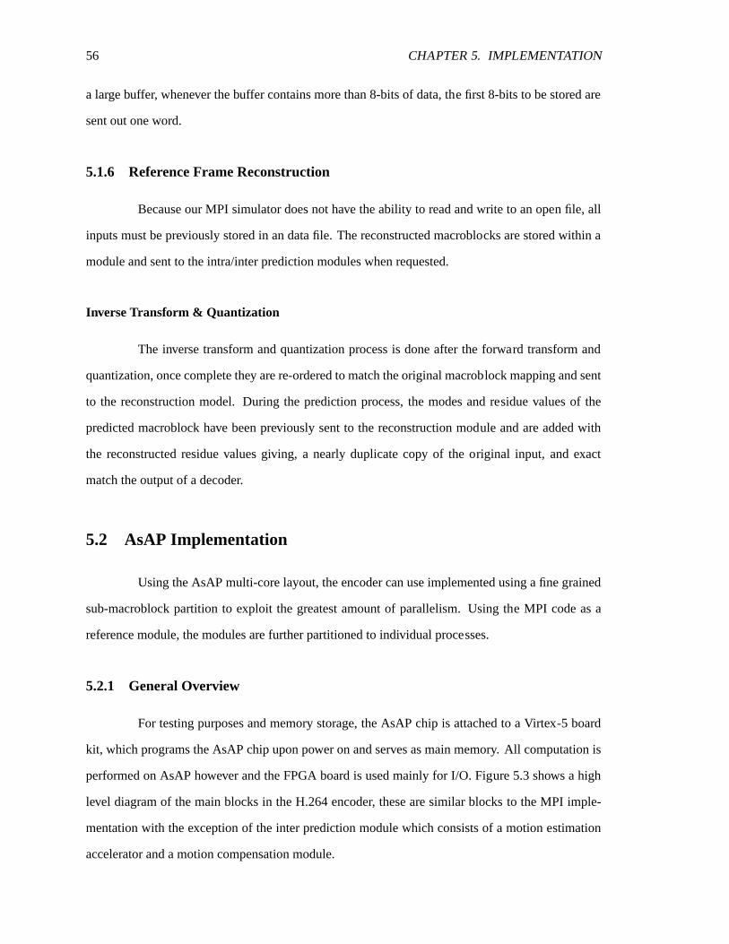
56 CHAPTER 5. IMPLEMENTATION
a large buffer, whenever the buffer contains more than 8-bits of data, the first 8-bits to be stored are
sent out one word.
5.1.6 Reference Frame Reconstruction
Because our MPI simulator does not have the ability to read and write to an open file, all
inputs must be previously stored in an data file. The reconstructed macroblocks are stored within a
module and sent to the intra/inter prediction modules when requested.
Inverse Transform & Quantization
The inverse transform and quantization process is done after the forward transform and
quantization, once complete they are re-ordered to match the original macroblock mapping and sent
to the reconstruction model. During the prediction process, the modes and residue values of the
predicted macroblock have been previously sent to the reconstruction module and are added with
the reconstructed residue values giving, a nearly duplicate copy of the original input, and exact
match the output of a decoder.
5.2 AsAP Implementation
Using the AsAP multi-core layout, the encoder can use implemented using a fine grained
sub-macroblock partition to exploit the greatest amount of parallelism. Using the MPI code as a
reference module, the modules are further partitioned to individual processes.
5.2.1 General Overview
For testing purposes and memory storage, the AsAP chip is attached to a Virtex-5 board
kit, which programs the AsAP chip upon power on and serves as main memory.All computation is
performed on AsAP however and the FPGA board is used mainly for I/O. Figure 5.3 shows a high
level diagram of the main blocks in the H.264 encoder, these are similar blocksto the MPI imple-
mentation with the exception of the inter prediction module which consists of a motion estimation
accelerator and a motion compensation module.
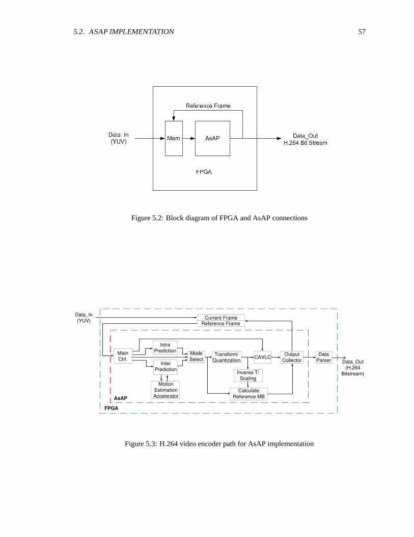
5.2. ASAP IMPLEMENTATION 57
D a t a _ I n( Y U V ) D a t a _ O u tH . 2 6 4 B i t S t r e a mA s A PM e m F P G AR e f e r e n c e F r a m e
Figure 5.2: Block diagram of FPGA and AsAP connections
Main
Ctrl.
Intra
Prediction
Inter
Prediction
Mode
SelectTransform/
Quantization
Inverse T/
Scaling
CAVLC
Reference Frame
Data_In
(YUV)
Data_Out
(H.264
Bitstream)
Output
Collector
Calculate
Reference MB
Data
Parser
Current Frame
Motion
Estimation
AcceleratorAsAP
FPGA
Figure 5.3: H.264 video encoder path for AsAP implementation
58 CHAPTER 5. IMPLEMENTATION
Mem Vit
Motion
Est.Mem Mem
data
request
VddHigh
VddLow
VddAlwaysOn
VddOsc
DVFS
OSC
VddCore
clock
valid
data
request
clock
valid
FFT
Core
Figure 5.4: Partition of H.264 modules on AsAP chip
5.2.2 Memory Organization
Three memory intensive task in the H.264 encoding process are the current/reference
frame management, motion vector management, and non-zero coefficient management. They arise
from the fact that encoding is based not only on the current macroblockbut also previously encoded
ones.
Current/Reference Frame Management
Each frame being encoded must be buffered to ensure that no data is lost,because of the
size of a picture frame, this data is stored off chip in FPGA memory, this also allows for future work
on larger than 1080p resolution pictures without any changes to the AsAP programs. After each
frame is encoded, it must also be saved for motion vector prediction in the next frame. The FPGA
memory is divided into three banks as shown in Fig. 5.7. Bank 0 holds the current frame, bank 1
holds the reconstructed current frame, and bank 2 holds the previouslyreconstructed frame. After
each frame the bank pointers are incremented so that the reconstructed frame that was in bank 1
now becomes the reference frame, data is read into bank 2, and the reconstructed data is in bank 0.

5.2. ASAP IMPLEMENTATION 59
Mem Vit
Motion
Est.Mem Mem
data
request
VddHigh
VddLow
VddAlwaysOn
VddOsc
DVFS
OSC
VddCore
clock
valid
data
request
clock
valid
FFT
Core
Figure 5.5: Partition of processors type on AsAP

60 CHAPTER 5. IMPLEMENTATION
Data
Collecotrtemp
Cb/Cr
Residue
Cb/Cr
H/V
Cb/Cr
Reorder
Cb/Cr
Temp
Main
ControlRedirect
Intra
Control
Intra
Memory
Cb/Cr
Cb/Cr
DC
1
SPS
PPS
Slice
HeaderRouter Router
MB
Request
Collector
Ref_Y_0
Intra Y
Memory
1
Intra Y
Memory
2
Router
Cb/Cr
DC
2
Intra
Mode
Pred.
MV
Pred
Ref_Y_2 Ref_Y_1
Intra
Memory
Control
16x16
DCRouter Router
4x4
DC
Pred
16x16
Pred 2
16x16
Pred 1Router
Ref_Y_3 Ref_Y_4
16x16
Residue
_1
16x16
H/VRouter Router
4x4
DC
Residue
DC
Pred
4x4
Pred 1
4x4
Pred 2
Recon.
MB
Inverse
Tx
Residue
2
Ref_Y_6 Ref_Y_5
16x16
Residue
_2
4x4
ResidueRouter Router
4x4
Vertical
Vertical
Pred.
Re-order
Residue
Inverse
Tx
Residue
1
Ref_Y_7 Router RouterReorder
ResidueRouter
4x4
Horiz.
Horiz.
Pred.Router Router
Inverse
Tx
Ref_Y_8
Test
Generat
or
Residue
1
Residue
2
16x16
Dequant
2x2
Dequant
AC
Rescale
Cur_Y Ref_C_0ITx
Start
QP
Table
4x4
ITx
Zig Zag
2
CAVLC
Scan 2
Data
Temp
Ref_C_2 Ref_C_14x4 AC
1
4x4 AC
2
Zig Zag
1
CAVLC
Scan 1sign 1's
total
zero
non zero
run
Ref_C_3 Ref_C_4Data
Request
2x2
HTx
2x2
Quant
Data
Receiver
num_co
effRouter Router Router
Calc_MB
Req.
Inter
Control
Calc.
SADCalc MV
16x16
HTx
16x16
Quant.
Level
Code 1
Level
Code 2
CAVLC
Out
Luma
Pred
nnz 2
ME
ControlCalc MV
CbCr
Pred.
nnz
Luma
Pred.
nnz 1
16K Memory
ME_ACC
16K Memory16K Memory
Pred.
Val.
Residue
Output
Figure 5.6: Links for communication between AsAP processors

5.2. ASAP IMPLEMENTATION 61C u r r e n t F r a m eB a n k 0R e f e r e n c e F r a m e 0B a n k 1R e f e r e n c e F r a m e 1B a n k 2M B D a t aM B R e q u e s t
Figure 5.7: Current/reference frame managment of AsAP implementation
Macroblock Management
Within the FPGA memory, data is stored according to macroblocks as shown in Fig. 5.8
with luma data first followed by chroma data. When a data request is make all 384 bytes of luma
and chroma data are sent at once. The only logic in the FPGA is a small memory controller for
where data should be stored. This can be implemented by using simple counter to keep track of the
start address for each macroblock.
Motion Vector Management
The H.264 standard supports sub-partitions of blocks for inter prediction, with two motion
vectors per block this becomes a possible maximum of 32 motion vectors when using the smallest
partition size(16 4x4 blocks). For motion vector prediction the preceding row of macroblock mo-
tion vectors must be saved. For 1080p-resolution, this would be a maximum of3840 words. For
simplicity all motion vectors for a macroblock are save even though only motion vectors that are on
the bottom of a macroblock are needed, hence the mode for each macroblock must also be stored
adding an additional 120 word for 1080p support. The block mode and motion vectors are stored in
BigMem with the first 500 address allocated for block mode and the remaining address for motion
vector data. The motion vector data is addressed in increment of 32 words,hence the MV for the
first macroblock is stored starting at address 500 and the MV for macroblock 2 is stored starting at
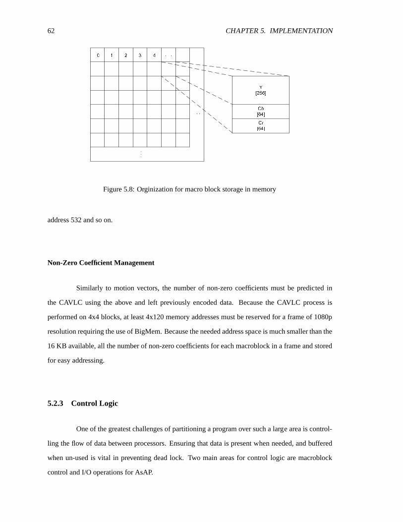
62 CHAPTER 5. IMPLEMENTATION
. . .0 1 2 3 4 . . .
...Y[ 2 5 6 ]C b[ 6 4 ]C r[ 6 4 ]
Figure 5.8: Orginization for macro block storage in memory
address 532 and so on.
Non-Zero Coefficient Management
Similarly to motion vectors, the number of non-zero coefficients must be predicted in
the CAVLC using the above and left previously encoded data. Because the CAVLC process is
performed on 4x4 blocks, at least 4x120 memory addresses must be reserved for a frame of 1080p
resolution requiring the use of BigMem. Because the needed address space is much smaller than the
16 KB available, all the number of non-zero coefficients for each macroblock in a frame and stored
for easy addressing.
5.2.3 Control Logic
One of the greatest challenges of partitioning a program over such a large area is control-
ling the flow of data between processors. Ensuring that data is present when needed, and buffered
when un-used is vital in preventing dead lock. Two main areas for controllogic are macroblock
control and I/O operations for AsAP.

5.2. ASAP IMPLEMENTATION 63
Macroblock Control
Video encoding is done on a macroblock basis, however to ensure that thedecoding path
produces the same data as the encoding path, prediction can only be done with previously encoded
blocks. For intra prediction this requires each macroblock to go through theintra prediction pro-
cess, integer transform, quantization, scaling, inverse transform, and reconstruction before the next
macroblock can be predicted. At each step proper control information must be present to ensure ac-
curacy. The chroma prediction process is much faster than luma prediction and the predicted value
used must be buffered prior to being sent to the reconstruction blocks to prevent a dead lock situation
at the integer transform. Because input FIFOs to each processor are only 64 words deep and chroma
data is 128 words for both Cb and Cr components, the chroma prediction processors will halt and
not send data to the integer transform while waiting the reconstruction processor to complete. How-
ever the reconstruction processor must wait for inverse transformed data before reconstructing the
reference frame thus causing a dead lock situation.
Basic macroblock and frame information is also sent along at each stage to ensure accu-
racy and increase code reuse. Parameters such as frame width, frame height, macro block width
(frame width /16), macro block number, encoding mode (intra/inter), block mode, and macNo %
macWidth (macro block number mod macro blocks width) are used at nearly every stage and trans-
mitted to save limited IMEM having to used to recompute these values. Many processors can start
some initial computation without all of the current data being present, this however requires that the
control information be broadcasted to many processors via long distance interconnects creating an
additional mapping issue.
External Memory Request & NAL
Because AsAP has only one input and one output link for communication with the FPGA,
both macroblock requests and the encoded .h264 bitstream must come from the same output. For
this the protocol in Table 5.1 is used. On the FPGA side a small block must also bepresent to parse
the data depending on the control bits, this however is rather simple and can be done in a few lines
of code. The protocol given will work with frame sizes up to 1080p, beyond this however each
request will need to consist of multiple 16-bit words in order to provide addressing for a greater

64 CHAPTER 5. IMPLEMENTATION
Bit Field Field Name Description
15:14 Control Bits 00: Write to output, payload contains H.264 output
01: Read from memory bank 0
payload contains macroblock number requested
10: Read from memory bank 1
payload contains macroblock number requested
11: Write to memory bank 2, payload contains pixel data
13:0 Payload For control bits 00 and 11: only bits 7:0 are used
For control bits 01 and 10
13:0 are used to request up to macroblock number 1023
Table 5.1: Output format for AsAP H.264 video encoder
I n t r aP r e d i c t i o nD a t a _ I nC o n t r o l _ I nR e q u e s t /C o m p l e t e M BR e s d uP r e d i c t e dM B
Figure 5.9: High level diagram of intra prediction in AsAP
number of macroblocks.
5.2.4 Intra Prediction
The intra prediction process although generally used only once per sequence constitutes
a rather large amount of computation. Figure 5.9 shows a high level block diagram for the intra
prediction module. Datain and controlin contain information for the current macroblock being
predicted, the requestMB signal is for requesting neighboring macroblock used for prediction.The
residue output goes to a re-ordering processor for the integer transform process and the predicted
macroblock goes to the reconstruction processor to be added to the reconstructed residue data.

5.2. ASAP IMPLEMENTATION 65
I n t r aC o n t r o lC h r o m aD a t a
L u m aD a t a
C h r o m aD CC h r o m aH o r z . / V e r t4 x 4D C4 x 4V e r t i c a l4 x 4H o r i z o n t a l1 6 x 1 6D C1 6 x 1 6H o r z . / V e r t .
C h r o m aR e s d u&P r e d i c t e dV a l u e
L u m aR e s d u&P r e d i c t e dV a l u eFigure 5.10: Block diagram of Intra prediction in AsAP
Parallelized Luma Prediction
Luma prediction can be done for both 16x16 and 4x4 blocks modes at the same time,
furthermore each prediction mode can also be done in parallel. In this implementation a processor
holds the current data to be predicted which is read by all processors doing prediction. Figure 5.10
shows how these blocks can be divided into parallel task. Each processor has a local copy of the
above and left macroblock and accesses the current data through a shared network.
When mapped to individual processors, half the processors are usedfor routing as shown
in Fig. 5.11. As explained in chapter four these routing processors are required to over come the
input limitation of each processor and to limit the number of processors being used for memory
storage. Here two processors are used to store luma data (256 8-bit words), this can be done in
one processor if data is compacted to 16-bit words, however two processors are used to reduce

66 CHAPTER 5. IMPLEMENTATION
addressing complexity.
Parallelized Chroma Prediction
Similar to luma prediction chroma prediction can also be parallelized as shown in Fig. 5.10.
Because there are only 64 Cb and 64 Cr data only one processor is needed for storage while 3 are
used for computation. To reduce the number of routing processors needed, data is automatically
sent to the DC mode computation processors for computing the SAD for each mode and requested
individually on the second pass for computing residue. In the first pass only Cb data is used for
computing the prediction mode. In the second pass both Cb and Cr are used for residue calculation.
Since chroma prediction is much smaller and faster than luma prediction the extra timeused by the
chroma prediction processors to compute the SAD first then residue the second time is acceptable.
5.2.5 Inter Prediction
Inter prediction is a computationally intensive task that is done on the majority of frames/slices.
To provide higher throughput AsAP uses a programmable motion estimation accelerator for this. A
high level diagram of the MEACC interface with neighboring processors is shown in Fig. 5.13.
Search Window Management
The ME ACC is capable of holding a 4x4 macroblock region for the search window.To
speed up the prediction process however only a 3x3 search window is used. The fourth column
can be used to pre-load data for the next prediction cycle, however the addressing scheme for this
becomes rather complex and is not easily done in a single processor. Herea new search window
is loaded from main memory for every macroblock. Although this is time consuming,it allows for
much simpler code. Each macroblock when read into the MEACC is also stored locally on one of
11 processors so that only 3 new macroblocks need to be read in from mainmemory.
Diamond Search Algorithm
A modified diamond search algorithm is use for all block sizes. The modified algorithm
uses only 5 search points as opposed to the nine points generally tested, and is repeated 4 times

5.2. ASAP IMPLEMENTATION 67
M e m o r y1 M e m o r y2 R o u t e r 1R o u t e r 2
R o u t e r 3R o u t e r 4
R o u t e r 5 4 x 4 D CP r e d i c t i o n4 x 4 D CR e s d u
4 x 4V e r t i c a l4 x 4H o r i z o n t a l
R o u t e r 6R o u t e r 7R o u t e r 8
1 6 x 1 6D C1 6 x 1 6H o r i z o n t a lV e r t i c a l
4 x 4R e s d u1 6 x 1 6R e s d u 11 6 x 1 6R e s d u 2
M e m o r yC o n t r o l
R e � O r d e rR e s d uR o u t e r 9Figure 5.11: Processor mapping for intra prediction in AsAP
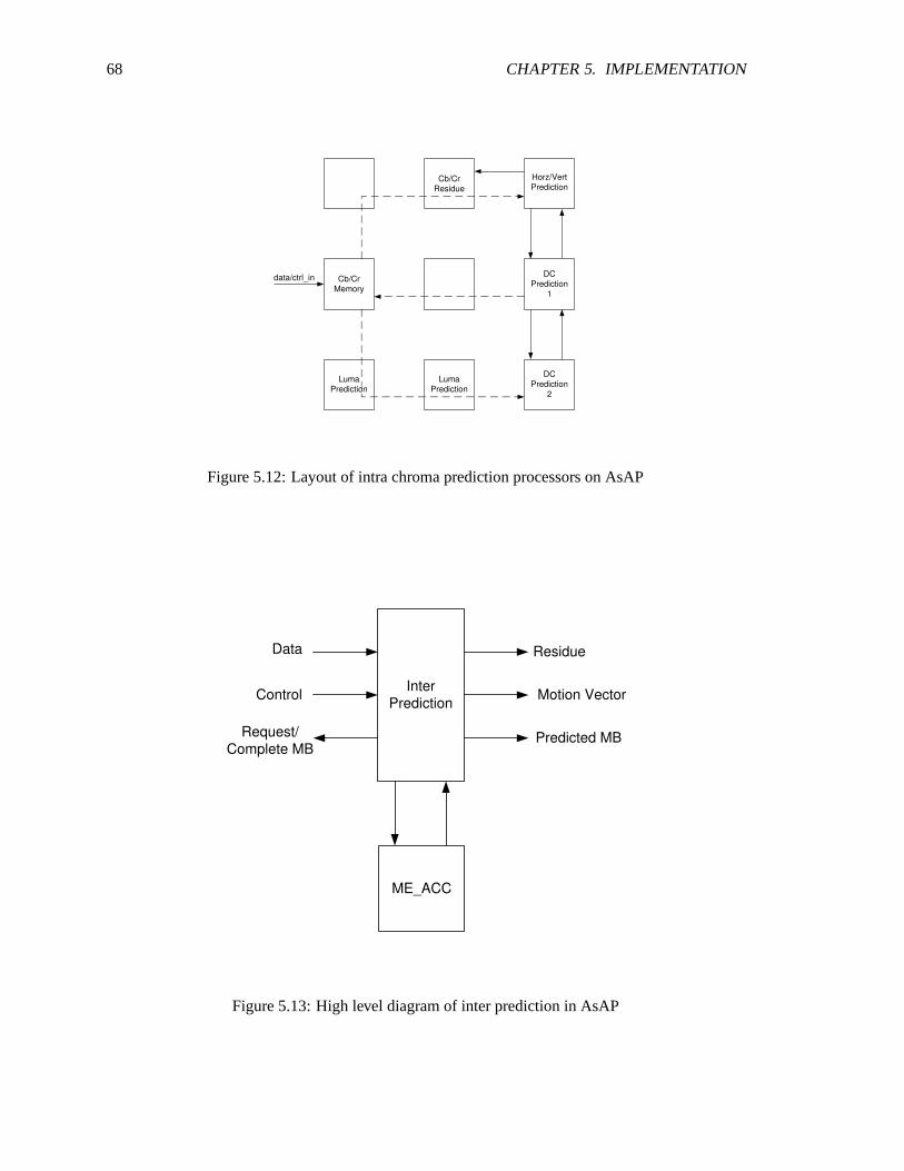
68 CHAPTER 5. IMPLEMENTATION
Cb/Cr
Memory
Cb/Cr
Residue
Horz/Vert
Prediction
DC
Prediction
1
DC
Prediction
2
Luma
Prediction
Luma
Prediction
data/ctrl_in
Figure 5.12: Layout of intra chroma prediction processors on AsAP
Inter
Prediction
Data
Control
Request/
Complete MB
Residue
Predicted MB
Motion Vector
ME_ACC
Figure 5.13: High level diagram of inter prediction in AsAP
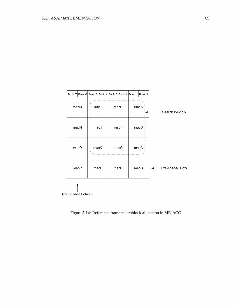
5.2. ASAP IMPLEMENTATION 69
m a c Bm a c Cm a c D
m a c Am a c Em a c Fm a c Gm a c H
m a c Im a c Jm a c Km a c L
m a c Mm a c Nm a c Om a c P
B a n k _ 0B a n k _ 1B a n k _ 2B a n k _ 3B a n k _ 4B a n k _ 5B a n k _ 6B a n k _ 7 S e a r c h W i n d o w
P r e K L o a d e d R o wP r e K L o a d e d C o l u m n
Figure 5.14: Reference frame macroblock allocation in MEACC

70 CHAPTER 5. IMPLEMENTATION
1 1 11111 1 122233 3 334 44 4
Figure 5.15: Diamond search pattern for motion estimation
to find the best match. Although this process is not as accurate as a full diamond search the only
drawback would be slightly higher entropy values to be encoded. This is generally not significant
unless there is a great difference in motion between frames, generally the majority of a frame is
constant or near constant.
Residue Calculations
Once the best set of motion vectors are computed, they are sent to a residue calculation
processor. The data used for this prediction is read from the 11 processors that hold a mirror copy
of the ME ACC memory. A block diagram of this can be seen in Fig. 5.16 along with the AsAP
layout is shown in Fig. 5.17.
5.2.6 Integer Transform & Quantization & Entropy Coding
Integer transform and quantization are done in similar fashion to the MPI-C model with
the exception that the integer transform path is replicated once with each pathtaking half of the
blocks to be encoded. Figure 5.18 shows the block diagram for this and Fig. 5.19 shows the proces-
sor layout.

5.2. ASAP IMPLEMENTATION 71
AsAP Processor Memory
Inter
Pred
Control
Calculate
SAD
Calc.
Residue
Predict
MV
ME_ACC
ME_ACC
Ctrl
data_in
ctrl_in
mb_request
residue_out
mvd_out
Figure 5.16: Block diagram of inter prediction module in AsAP
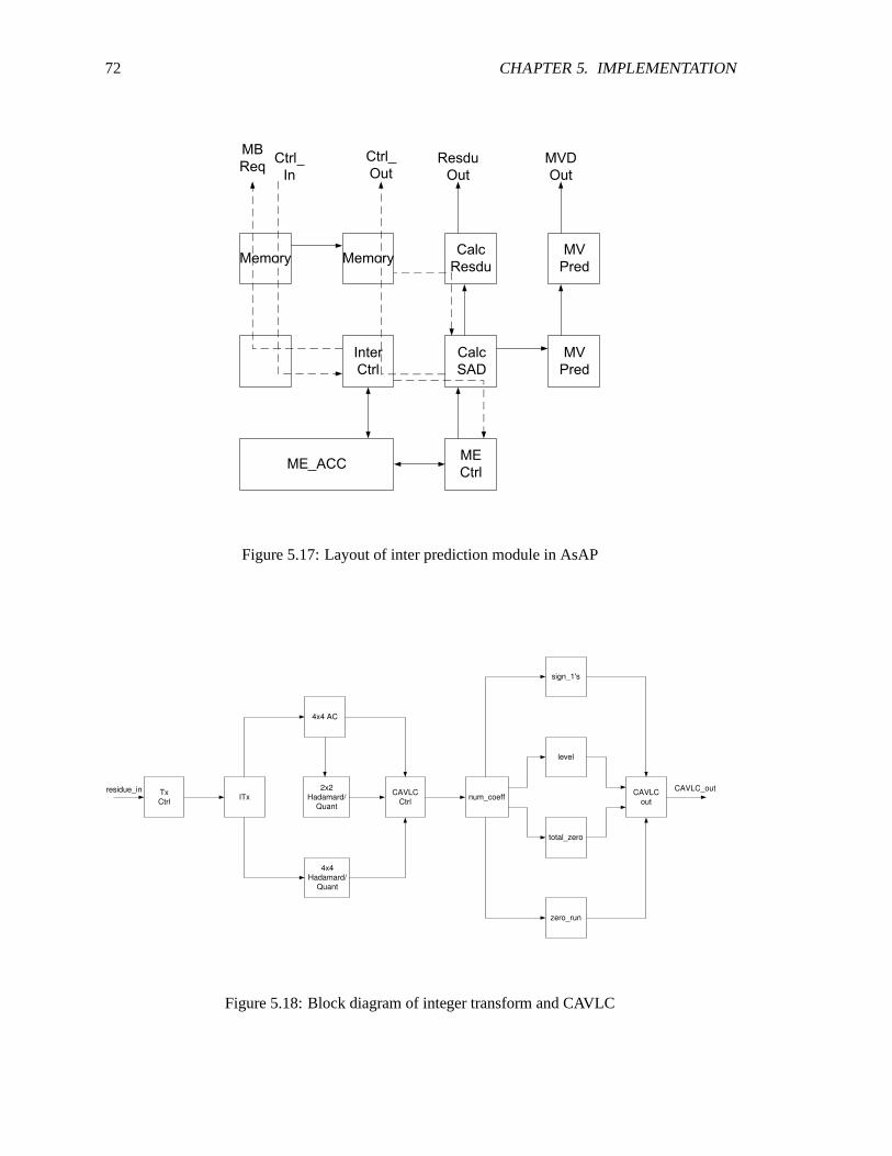
72 CHAPTER 5. IMPLEMENTATION
Figure 5.17: Layout of inter prediction module in AsAP
Tx
CtrlITx
4x4 AC
2x2
Hadamard/
Quant
4x4
Hadamard/
Quant
CAVLC
Ctrl
sign_1's
level
total_zero
zero_run
CAVLC
outnum_coeff
CAVLC_outresidue_in
Figure 5.18: Block diagram of integer transform and CAVLC
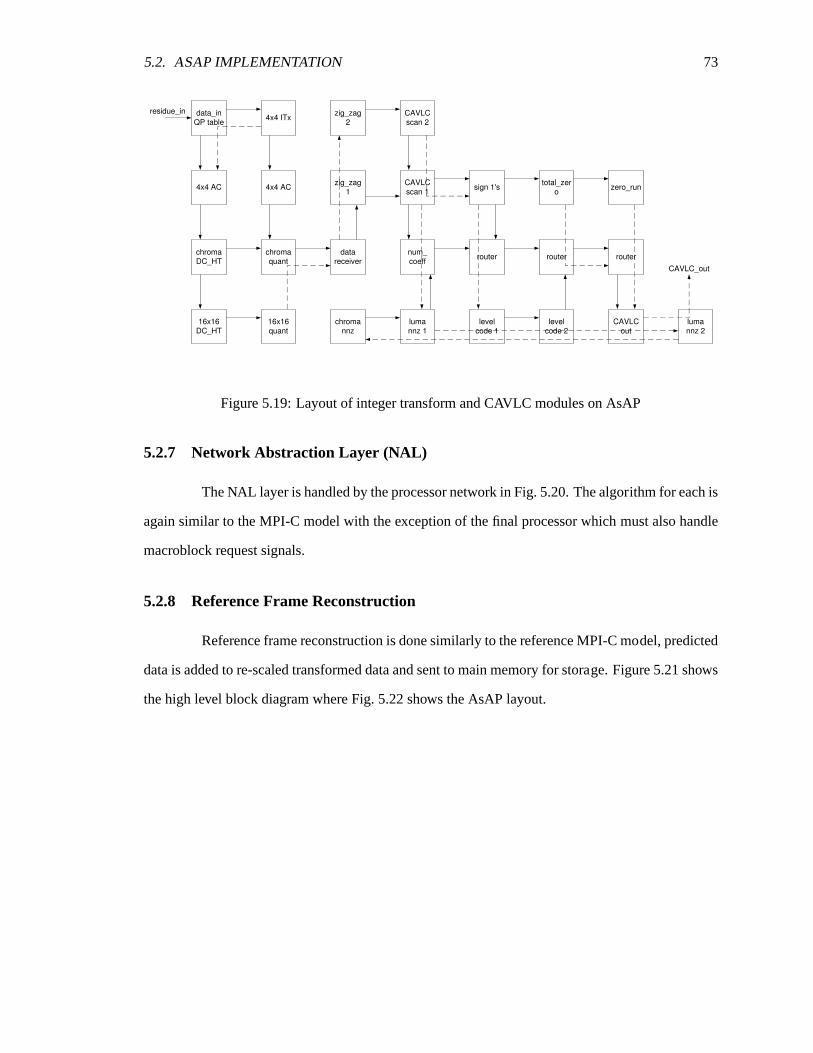
5.2. ASAP IMPLEMENTATION 73
data_inQP table
4x4 ITx
4x4 AC 4x4 AC
chromaDC_HT
chromaquant
16x16DC_HT
16x16quant
zig_zag1
datareceiver
chromannz
CAVLCscan 1
num_coeff
zig_zag2
CAVLCscan 2
lumannz 1
sign 1's
router
levelcode 1
total_zero
router
levelcode 2
zero_run
router
CAVLCout
lumannz 2
residue_in
CAVLC_out
Figure 5.19: Layout of integer transform and CAVLC modules on AsAP
5.2.7 Network Abstraction Layer (NAL)
The NAL layer is handled by the processor network in Fig. 5.20. The algorithm for each is
again similar to the MPI-C model with the exception of the final processor whichmust also handle
macroblock request signals.
5.2.8 Reference Frame Reconstruction
Reference frame reconstruction is done similarly to the reference MPI-C model, predicted
data is added to re-scaled transformed data and sent to main memory for storage. Figure 5.21 shows
the high level block diagram where Fig. 5.22 shows the AsAP layout.

74 CHAPTER 5. IMPLEMENTATION
SPS
PPSSH Router Out
Intra
Mode
Coding
MV
CodingRouter
Ctrl_In
Reconstructed
DataCAVLC
Data
output
Figure 5.20: Layout of header module on AsAP
AC
Rescaling
Cb/Cr
Dequant
16x16 DC
Dequant
ITx Reconstruct
predicted MB
AC_in
Cb/Cr_in
DC_in
reconstructed
MB
Figure 5.21: Block diagram of reconstruction module
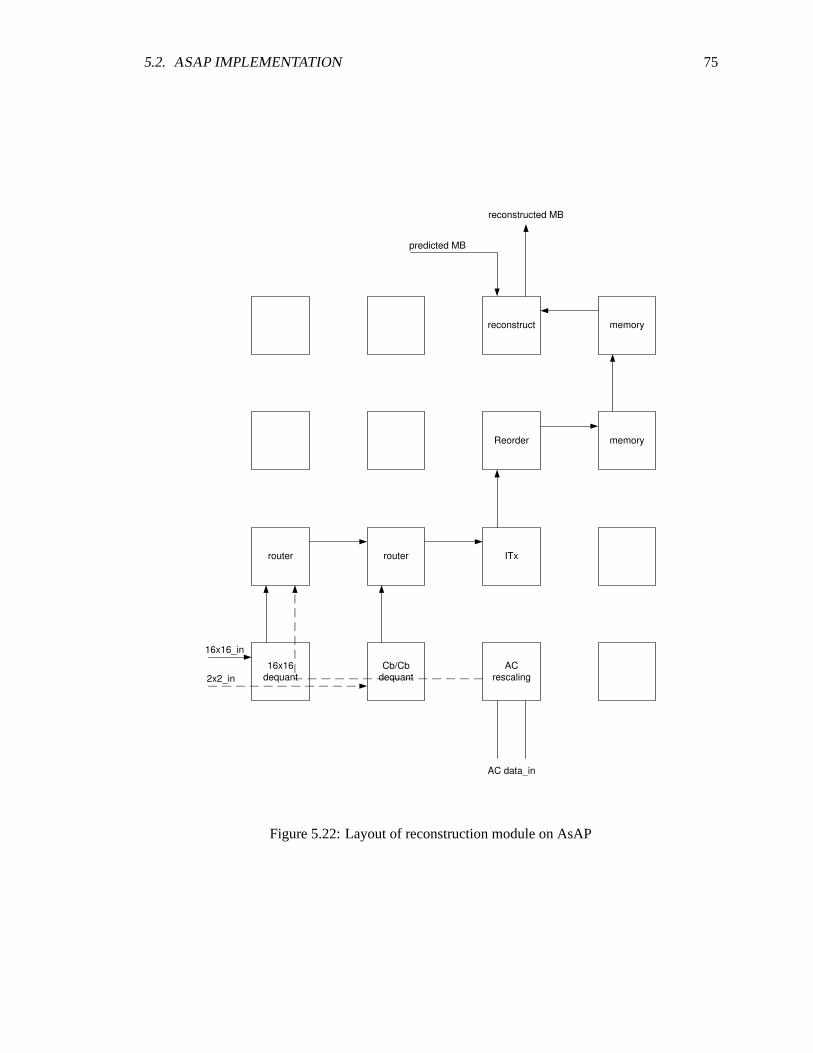
5.2. ASAP IMPLEMENTATION 75
16x16
dequant
Cb/Cb
dequant
AC
rescaling
router router ITx
Reorder memory
memoryreconstruct
predicted MB
reconstructed MB
AC data_in
16x16_in
2x2_in
Figure 5.22: Layout of reconstruction module on AsAP

76 CHAPTER 5. IMPLEMENTATION

77
Chapter 6
Results and Analysis
Initial results for the implemented H.264 encoder are gathered from simulation of the
AsAP chip in SimVision and NCVerilog. Results and data for analysis are gathered using assembler
functions that were able to measure the energy, traffic, and activity of each processor. Section 6.1
presents the metrics used for testing and analysis, section 6.2 gives a comparison of the encoder
with other implementations, and section 6.3 gives an analysis of the encoder onthe AsAP chip.
6.1 Metrics for Testing and Analysis
For an accurate analysis of the encoder on the AsAP chip, the following metrics have been
considered:
• Program Size: The program size (instruction memory) and data memory of each computa-
tional and routing processor has been collected for analysis. Processors which are solely used
for long distance interconnects have been ignored.
• Energy: The energy of each processors is measured. The energy measurements consists of
the average power per cycle of the MAC, ALU, Branch, FIFO read/write, and NOP/stall as
measured in lab. In simulation, as each instruction is processed, the corresponding average
energy is added to the total. The activity of each processor is also recorded, and used for an
estimate of the energy consumption.
• Speed: The speed of each processors is initially set to the maximum frequency to get the
78 CHAPTER 6. RESULTS AND ANALYSIS
highest performance. For minimum energy consumption, the energy of each processor can be
scaled later.
• Communication: Links between every processors will be analyzed for theircommunication
distance and average throughput.
Accuracy
The encoded data is compared to the reference output of the MPI-C output for accuracy.
For smaller frame sizes the .h264 output bitstream can also be decoded usingthe reference software
JM, and compared using Elecard YUV viewer. Because of the encoding algorithm implemented,
the encoder is nearly data independent. In intra prediction regardless ofthe input data, all processors
doing prediction will execute the same set of instructions except for the processor calculating the
chosen prediction will repeat its calculation again. Although a different mode may be chosen every
time, the number of instruction repeated in any of the processors is very similarand will yield
the same approximate power. In inter prediction, the MEACC will undergo the same number of
iterations every time, the only variance will be in the motion vector prediction. In the motion vector
prediction depending on the mode, different conditions are taken but the number of instructions
per condition is approximately equal and will have little effect on the overall accuracy. Simulation
setup time is not a factor for intra prediction, at the start of every macroblock the pipeline will be
empty because prediction cannot start until the previous prediction is complete, essentially starting
over every time. In inter prediction, the only overlap of computation between macroblocks is in the
integer transform and CAVLC phases, both of which are much shorter and less power consuming
than the prediction process thus will not have a significant effect on results. To account for this
though a much longer simulation time is used so that this small factor can be averaged out.
Video Sequences (Size and Length)
Because of the limitation of the simulator, representative macroblocks are chosen and
the results are interpolated for the entire frame. The average time for a macroblock to be encoded
is calculated from the time it is requested to the time the reference frame is completedin intra
prediction and from the time requested to when the MEACC completes the search pattern for inter
6.2. PERFORMANCE COMPARISONS 79
prediction. This is then multiplied by the number of macroblocks per frame to determining the
number of frames per second the encoder is capable of for the given frequency and voltage.
6.2 Performance Comparisons
Performance comparison is broken down into two categories, intra frames and inter frames,
in each situation the simulated results of a few macroblock are used to interpolatethe data for each
frame. Two different comparison are given depending on the frame sizes, general purpose and pro-
grammable processors are compared for smaller frame sizes only since the performance of these
types of platforms do not allow for encoding of larger frame sizes. Since data is only presented for
a few frame sizes, the number of frames per second has been interpolatedfor various other frame
sizes for comparison based on the number of macroblocks that can be encoded per second. The
operation frequency has been kept the same as in the original implementation.Since ASICs are
built specifically for encoding and have been optimized only, know data is presented. The reported
memory size is for internal memory only, depending on the platform, the encoders may also use
additional off-chip memory, please refer for the references for a moredetailed description of each.
Power is also only reported for larger frame sizes since no power/energy data is given in other
implementations for small frame sizes for comparison.
The encoder has also been implemented on the AsAP chip with bit accurate values as
compared to AsAP simulation and MPI simulation. Table 6.1 gives the maximum frequency and
encoded frames per second achieved with each given voltage and the corresponding power values.
Results of the encoder implementation on-chip is consistent with per-processor performance of the
AsAP2 chip as presented in the IEEE Journal of Solid-State Circuits with a few minor exceptions
[7]. The single processor speed when running at .675 V was 66 MHz and 1.2 GHz at 1.3 V. The
performance increase is not linear though, at speeds beyond 1 GHz, the performance increase begins
to level off, possibly due to power grid noise and velocity saturation in the device. The max speed
achieved in the H.264 encoder at 1.3 V was about 800 MHz, approximately a30% reduction in speed
but with linear increases in performance as voltage is increased. Variousfactors may be contributing
to the lower performance, most notably the stress on the power grid from running 115 processors
simultaneously as opposed to a single processor. The encoder performance and behavior though are

80 CHAPTER 6. RESULTS AND ANALYSIS
Voltage Max Frequncy Intra Inter Power Power
(V) (MHz) fps (QCIF) fps (QCIF) Intra (mW) Inter (mW)
0.8 172 19 95 108.8 365.1
0.9 295 33 160 213.6 452.6
1.0 410 49 233 419.0 662.3
1.1 539 66 324 696.3 908.4
1.2 651 82 427 802.7 1059
1.3 798 96 478 947.5 1189
Table 6.1: Performance of H.264 video encoder on AsAP2 chip
expected and consistent with single processor measurements. The maximum frequency achieved
increases linearly with increases in voltage as seen in the single processortest for frequencies below
1 GHz. The power measurements for the encoder are also within 30% of the expected power when
the measured per-processor power is multiplied by the number of active processors in the encoder.

6.2.P
ER
FO
RM
AN
CE
CO
MP
AR
ISO
NS
81
Platform Intel Xeon [4] Intel PXA27x [5] ADSP-BF561 [13] ARM [14] ASIC [15] ASIC [6] AsAP AsAP
(4 cores) (2 cores) 1136J-S intra inter
Technology (CMOS) 90nm - - - 180nm 180nm 65nm 65nm
Area (mm2) - 26.78 - - 31.72 27.1 18.87 19.2
Internal (KB) 256 KB (L2) - 328 - 34.7 64000 16 32
Memory 2MB (L3)
QCIF (fps) 18.4 * 49 218 * 15 - - 41 216
Frequency 2.8 GHz 624 MHz 600 MHz 69 MHz - - 1.2 GHz 1.2 GHz
CIF (fps) 4.6 12.25 * 54 * 3.75 * - - 10 54
Frequency 2.8 GHz 624 MHz 600 MHz 69 MHz - - 1.2 GHz 1.2 GHz
4CIF (fps) - - 13.6 * - 30 - 2 13.5
Frequency - - 600 MHz - 81 MHz - 1.2 GHz 1.2 GHz
Power (mW) - - - - 581 - 702 955
720p (fps) - - 6 * - 30 - - 5.94
Frequency - - 600 MHz - 108 MHz - - 1.2 GHz
Power (mW) - - - - 785 - - 955
1080p (fps) - - 2.7 * - - 25 - 2.64
Frequency - - 600 MHz - - 200 MHz - 1.2 GHz
Power (mW) - - - - - 1219 - 955
Table 6.2: Comparison of H.264 Encoders * These value are interpolated from given data based on the number of macroblocks that can be encodedper second
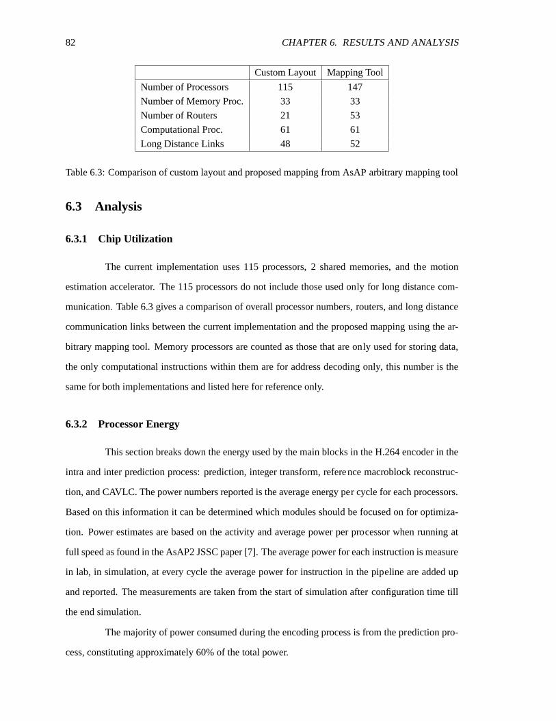
82 CHAPTER 6. RESULTS AND ANALYSIS
Custom Layout Mapping Tool
Number of Processors 115 147
Number of Memory Proc. 33 33
Number of Routers 21 53
Computational Proc. 61 61
Long Distance Links 48 52
Table 6.3: Comparison of custom layout and proposed mapping from AsAParbitrary mapping tool
6.3 Analysis
6.3.1 Chip Utilization
The current implementation uses 115 processors, 2 shared memories, and the motion
estimation accelerator. The 115 processors do not include those used only for long distance com-
munication. Table 6.3 gives a comparison of overall processor numbers,routers, and long distance
communication links between the current implementation and the proposed mappingusing the ar-
bitrary mapping tool. Memory processors are counted as those that are only used for storing data,
the only computational instructions within them are for address decoding only, this number is the
same for both implementations and listed here for reference only.
6.3.2 Processor Energy
This section breaks down the energy used by the main blocks in the H.264 encoder in the
intra and inter prediction process: prediction, integer transform, reference macroblock reconstruc-
tion, and CAVLC. The power numbers reported is the average energy per cycle for each processors.
Based on this information it can be determined which modules should be focused on for optimiza-
tion. Power estimates are based on the activity and average power per processor when running at
full speed as found in the AsAP2 JSSC paper [7]. The average powerfor each instruction is measure
in lab, in simulation, at every cycle the average power for instruction in the pipeline are added up
and reported. The measurements are taken from the start of simulation afterconfiguration time till
the end simulation.
The majority of power consumed during the encoding process is from the prediction pro-
cess, constituting approximately 60% of the total power.
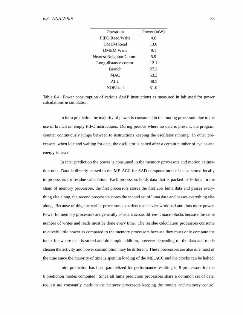
6.3. ANALYSIS 83
Operation Power (mW)
FIFO Read/Write 4.6
DMEM Read 13.0
DMEM Write 9.1
Nearest Neighbor Comm. 5.9
Long-distance comm. 12.1
Branch 27.2
MAC 53.3
ALU 48.5
NOP/stall 31.0
Table 6.4: Power consumption of various AsAP instructions as measured in lab used for powercalculations in simulation
In intra prediction the majority of power is consumed in the routing processorsdue to the
use of branch on empty FIFO instructions. During periods where no data ispresent, the program
counter continuously jumps between to instructions keeping the oscillator running. In other pro-
cessors, when idle and waiting for data, the oscillator is halted after a certainnumber of cycles and
energy is saved.
In inter prediction the power is consumed in the memory processors and motion estima-
tion unit. Data is directly passed to the MEACC for SAD computation but is also stored locally
in processors for residue calculation. Each processors holds data that is packed to 16-bits. In the
chain of memory processors, the first processors stores the first 256luma data and passes every-
thing else along, the second processors stores the second set of luma data and passes everything else
along. Because of this, the earlier processors experience a heavier workload and thus more power.
Power for memory processors are generally constant across different macroblocks because the same
number of writes and reads must be done every time. The residue calculationprocessors consume
relatively little power as compared to the memory processors because they must only compute the
index for where data is stored and do simple addition, however depending on the data and mode
chosen the activity and power consumption may be different. These processors are also idle most of
the time since the majority of time is spent in loading of the MEACC and the clocks can be halted.
Intra prediction has been parallelized for performance resulting in 9 processors for the
6 prediction modes computed. Since all luma prediction processors share a common set of data,
request are constantly made to the memory processors keeping the routersand memory control
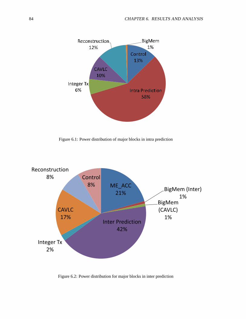
84 CHAPTER 6. RESULTS AND ANALYSIS
C o n t r o l1 3 %i o n
I n t e g e r6 %C A V L C1 0 %O t h e r2 9 % C o n t r o l1 3 %
I n t r a P r e d i c t i o n5 8 %I n t e g e r T x6 % C A V L C1 0 %R e c o n s t r u c t i o n1 2 % B i g M e m1 %
Figure 6.1: Power distribution of major blocks in intra prediction
Figure 6.2: Power distribution for major blocks in inter prediction
6.3. ANALYSIS 85
01 0 02 0 03 0 04 0 05 0 06 0 07 0 08 0 09 0 01 0 0 02 4 . 8 4 9 . 5 9 8 . 2 1 9 6 3 9 7 7 9 8P ower( mW)
F r e q u e n c y ( M H z )(a) Average power vs. frequency
02 04 06 08 01 0 01 2 02 4 . 8 4 9 . 5 9 8 . 2 1 9 6 3 9 7 7 9 8f ramespersecond
F r e q u e n c y ( M H z )(b) Encoded frames per second vs. frequency
Figure 6.3: Average power and number of encoded frames per secondvs. frequency at 1.3V onAsAP2 chip
processor router active most of the time. Data is requested twice for the 16x16 and 4x4 modes,
once to determine the SAD for each mode than again to compute the actual SAD. This was done
because the data memory for each processors is only 128 word and cannot store both the current
data, variables needed for prediction, and the predicted data. It is not know which block/mode will
be chosen till all blocks/mode are computed, saving the predicted value for each would consume
too much memory space.
Figure 6.10 shows the average power for processors in the reconstruction module for both
intra and inter prediction, one of the processors is shown as using no power because it is only used
for intra 16x16 prediction (the test case here uses intra 4x4 prediction, hence this block is not used
and only passes data which consumes very little power compared to other processors). In inter
prediction, because the prediction can continue once the SAD for each macroblock is computed, the
reconstruction module is used more often, however because data comes from one source only, few
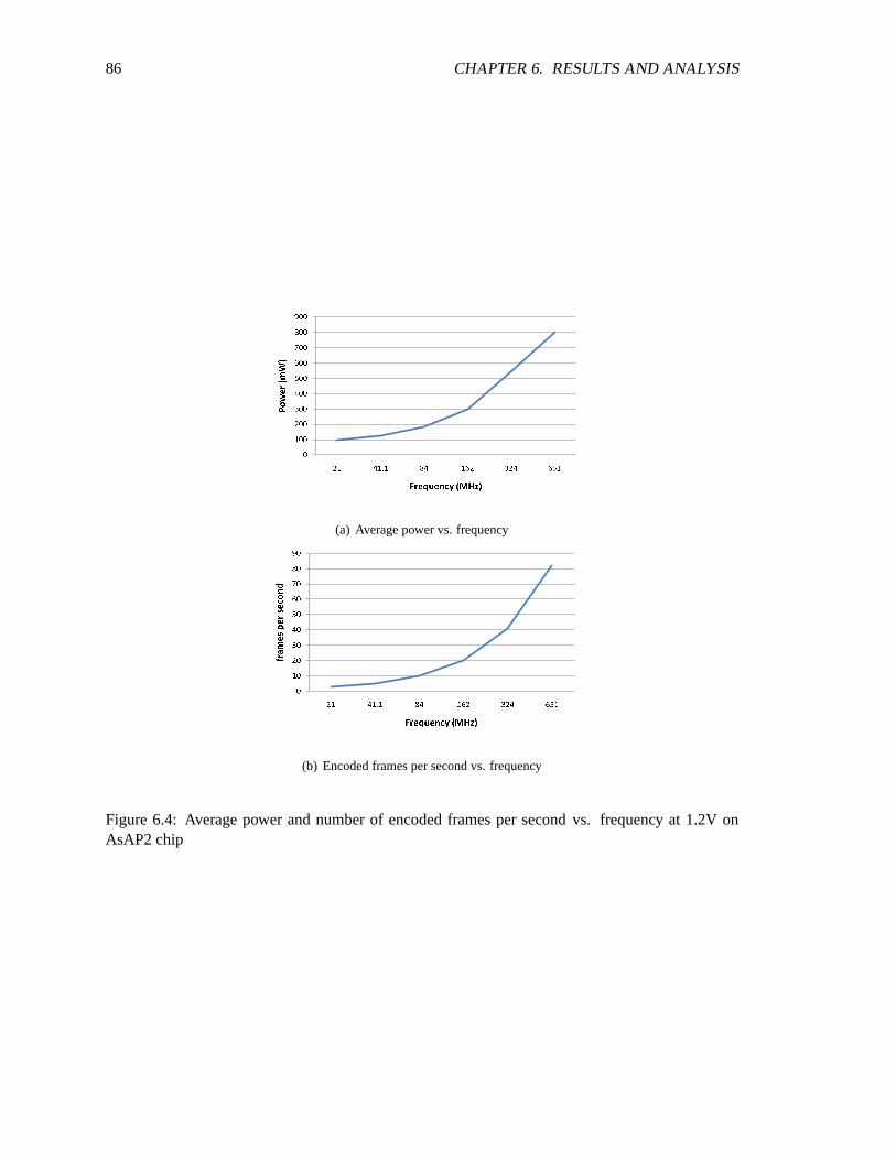
86 CHAPTER 6. RESULTS AND ANALYSIS
01 0 02 0 03 0 04 0 05 0 06 0 07 0 08 0 09 0 02 1 4 1 . 1 8 4 1 6 2 3 2 4 6 5 1P ower( mW)
F r e q u e n c y ( M H z )(a) Average power vs. frequency
01 02 03 04 05 06 07 08 09 02 1 4 1 . 1 8 4 1 6 2 3 2 4 6 5 1f ramespersecond
F r e q u e n c y ( M H z )(b) Encoded frames per second vs. frequency
Figure 6.4: Average power and number of encoded frames per secondvs. frequency at 1.2V onAsAP2 chip

6.3. ANALYSIS 87
01 0 02 0 03 0 04 0 05 0 06 0 07 0 08 0 01 6 . 9 3 3 . 3 6 4 1 4 5 2 6 2 5 3 9P ower( mW)
F r e q u e n c y ( M H z )(a) Average power vs. frequency
01 02 03 04 05 06 07 01 6 . 9 3 3 . 3 6 4 1 4 5 2 6 2 5 3 9f ramespersecond
F r e q u e n c y ( M H z )(b) Encoded frames per second vs. frequency
Figure 6.5: Average power and number of encoded frames per secondvs. frequency at 1.1V onAsAP2 chip

88 CHAPTER 6. RESULTS AND ANALYSIS
05 01 0 01 5 02 0 02 5 03 0 03 5 04 0 04 5 01 2 . 7 2 5 . 4 5 1 1 0 0 1 9 0 4 1 0P ower( mW)
F r e q u e n c y ( M H z )(a) Average power vs. frequency
01 02 03 04 05 06 01 2 . 7 2 5 . 4 5 1 1 0 0 1 9 0 4 1 0f ramespersecond
F r e q u e n c y ( M H z )(b) Encoded frames per second vs. frequency
Figure 6.6: Average power and number of encoded frames per secondvs. frequency at 1.0V onAsAP2 chip

6.3. ANALYSIS 89
05 01 0 01 5 02 0 02 5 08 . 7 1 7 . 2 3 3 . 3 6 6 . 7 1 4 1 2 9 5P ower( mW)
F r e q u e n c y ( M H z )(a) Average power vs. frequency
051 01 52 02 53 03 54 08 . 7 1 7 . 2 3 3 . 3 6 6 . 7 1 4 1 2 9 5f ramespersecond
F r e u q u e n c y ( M H z )(b) Encoded frames per second vs. frequency
Figure 6.7: Average power and number of encoded frames per secondvs. frequency at 0.9V onAsAP2 chip
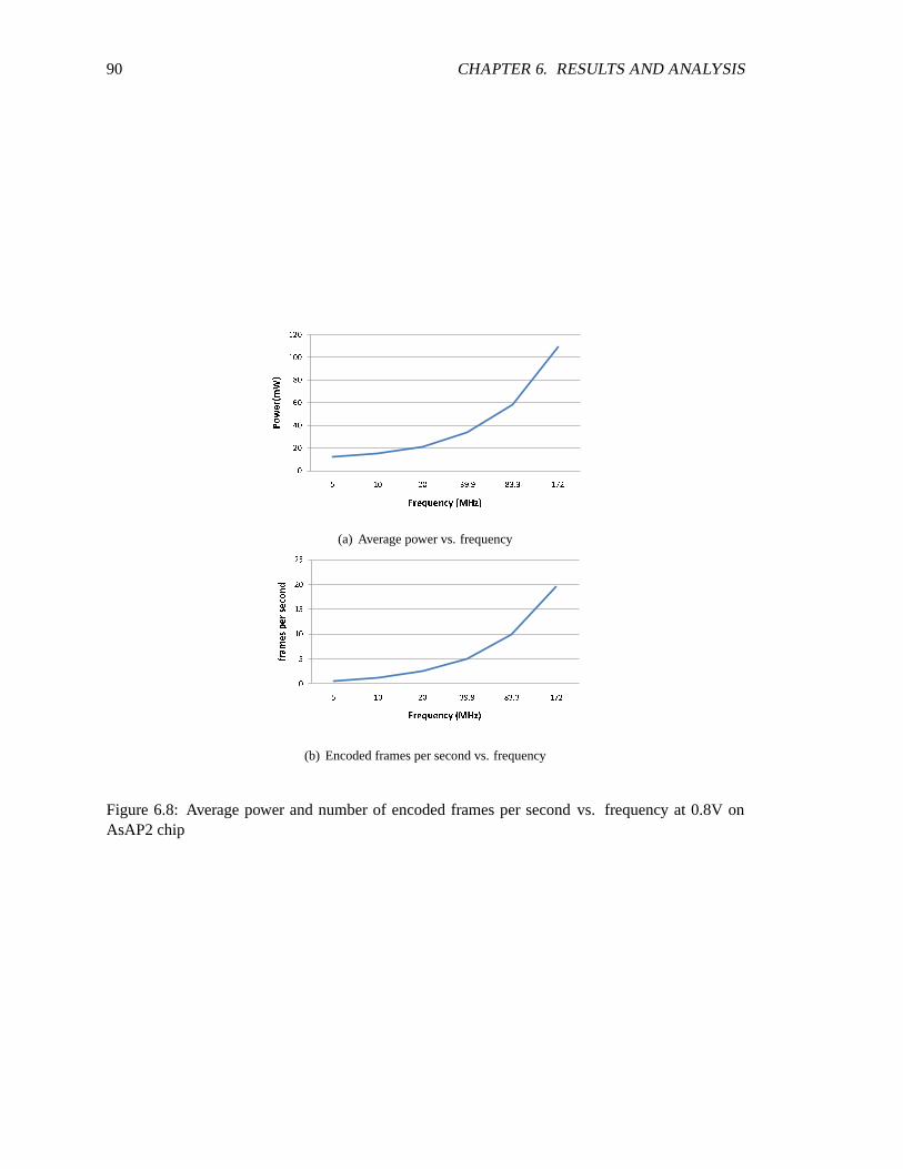
90 CHAPTER 6. RESULTS AND ANALYSIS
02 04 06 08 01 0 01 2 05 1 0 2 0 3 9 . 9 8 3 . 3 1 7 2P ower( mW)
F r e q u e n c y ( M H z )(a) Average power vs. frequency
051 01 52 02 55 1 0 2 0 3 9 . 9 8 3 . 3 1 7 2f ramespersecond
F r e q u e n c y ( M H z )(b) Encoded frames per second vs. frequency
Figure 6.8: Average power and number of encoded frames per secondvs. frequency at 0.8V onAsAP2 chip
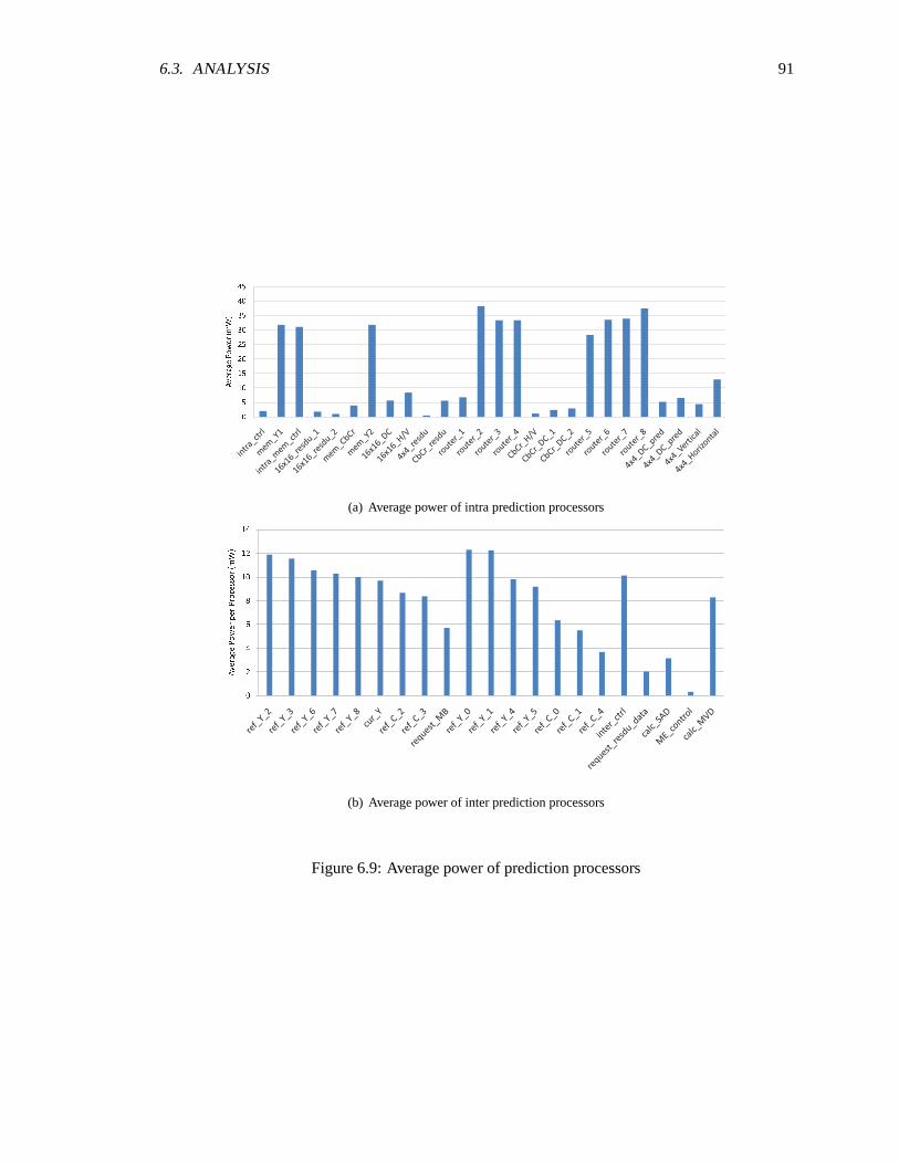
6.3. ANALYSIS 91
0 51 01 52 02 53 03 54 04 5A verageP ower( mW)
(a) Average power of intra prediction processors
024681 01 21 4
A verageP owerperP rocessor( mW)
(b) Average power of inter prediction processors
Figure 6.9: Average power of prediction processors
92 CHAPTER 6. RESULTS AND ANALYSIS
routing processors are used which the primary power consumers in the intra prediction process.
The majority of power used for integer transform is in routing for the intra prediction
mode, inputs are constantly scanned for which type of intra prediction mode isused. The actual
transform processors have been optimized by Zhibin [3] therefore consuming very little power. The
amount of time that these processors are active is also very small when compared to the entire
encoding process hence they are idle most of the time.
The CAVLC used in this work has also been previously optimized by Zhibin [3], some
changes were make to the prediction processes for non zero coefficients resulting in the much larger
power consumption. The power for each processor is data dependenthowever, so for another input
sequence the power difference may also be different. These processors can be optimized by either
code scheduling to reduce the number of no-ops used or DVFS.
Energy Overhead of Switching I/P Frames
The energy overhead associated with switching frame types is negligible since the only
difference would be that the SPS and PPS need to be resent which resultsin a average power of 129
uW for that processor. The only control change would be an additional8 lines of code inside the
main control processor which is negligible. This low switching cost is possible because the header
information is hardcoded and do not need to be recomputed.
6.3.3 Processor Utilization
Processor utilization is presented as the percentage of time the processorsis active, stalling
(when oscillator is on or off combined) on input, stalling on output, and stalling on no-ops. The ac-
tivity tracks closely with those of the power plots. The stall on no-ops can beeliminated through
code scheduling to hide latencies. By analyzing the stall on inputs/outputs, DVFS values can be cal-
culated for maximum utilization. The majority of stalls occur on reads where data from a previous
processor is needed, this arises from the fact that during intra prediction each macroblock must be
predicted, computed, transformed, and reconstructed before the nextmacroblock can begin. These
long periods of stalling generally do not consume too much power because the processor oscilla-
tors are halted after a certain period, the exception again are routing processors which continuously
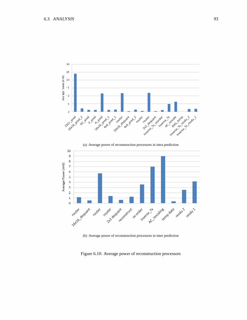
6.3. ANALYSIS 93
051 01 52 02 53 0A verageP ower( mW)
(a) Average power of reconstruction processors in intra prediction
0 1234567891 0
A verageP ower( mW)
(b) Average power of reconstruction processors in inter prediction
Figure 6.10: Average power of reconstruction processors

94 CHAPTER 6. RESULTS AND ANALYSIS
024681 01 21 4
A verageP ower( mW)
(a) Average power of processors for integer transform in intra prediction
00 . 20 . 40 . 60 . 811 . 21 . 41 . 61 . 82A verageP ower( mW)
(b) Average power of processors for integer transform in inter prediction
Figure 6.11: Average power of integer transform processors
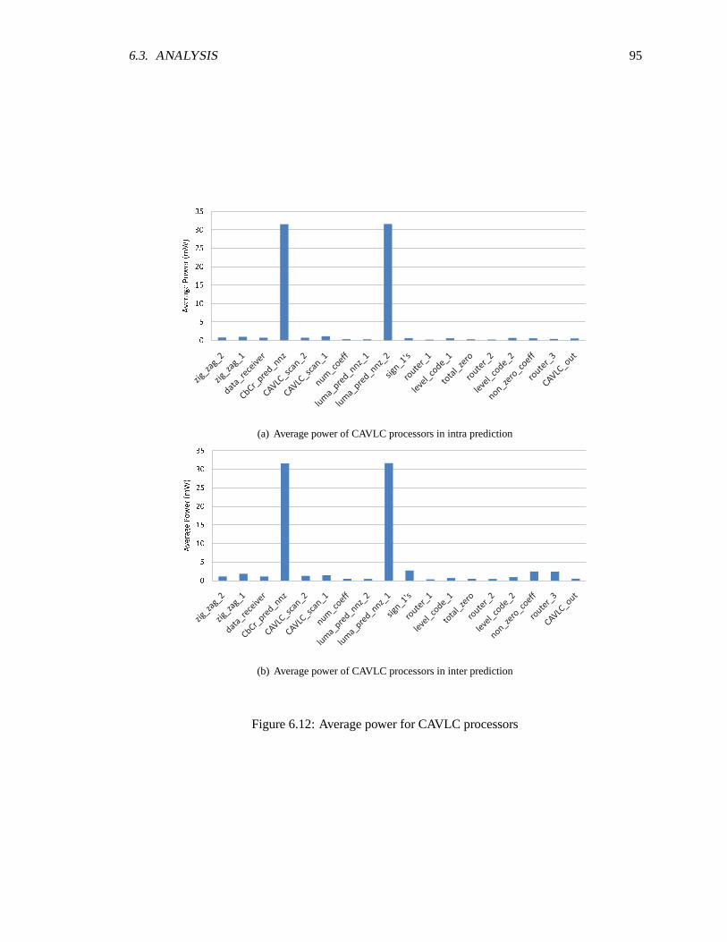
6.3. ANALYSIS 95
051 01 52 02 53 03 5A verageP ower( mW)
(a) Average power of CAVLC processors in intra prediction
051 01 52 02 53 03 5A verageP ower( mW)
(b) Average power of CAVLC processors in inter prediction
Figure 6.12: Average power for CAVLC processors

96 CHAPTER 6. RESULTS AND ANALYSIS
0 10 20 30 40 50 60 70 800
10
20
30
40
50
60
70
80
90
100
Pro
cess
or A
ctiv
ity (
%)
Figure 6.13: Average activity of processors used in intra prediction
0 10 20 30 40 50 60 700
10
20
30
40
50
60
70
80
90
100
Pro
cess
or A
ctiv
ity (
%)
Figure 6.14: Average Activity of processors used in inter prediction
branch between a few no-ops and branch on FIFO instructions. The indexes for the x-axis for these
plots correspond to the same functions as those shown for the power plots.
During the reconstruction phase, although the inverse transform process is also done on
a 4x4 block basis, they must be reordered prior to being transformed. Asshown in Fig. 6.15, the
first few processors hold the DC data and must wait for the forward integer transform process to
complete before starting, showing the stall on input. Once this is complete, the inverse transform
process is fairly simple consisting of mainly adds and shifts resulting in the majorityof time waiting
for more inputs.
Because the integer transform and CAVLC process are quick comparedto the prediction
process, the majority of time is spent idle waiting for more data to encode. For maximum optimiza-
tion these blocks are important, but the focus should be on the prediction blocks first because they
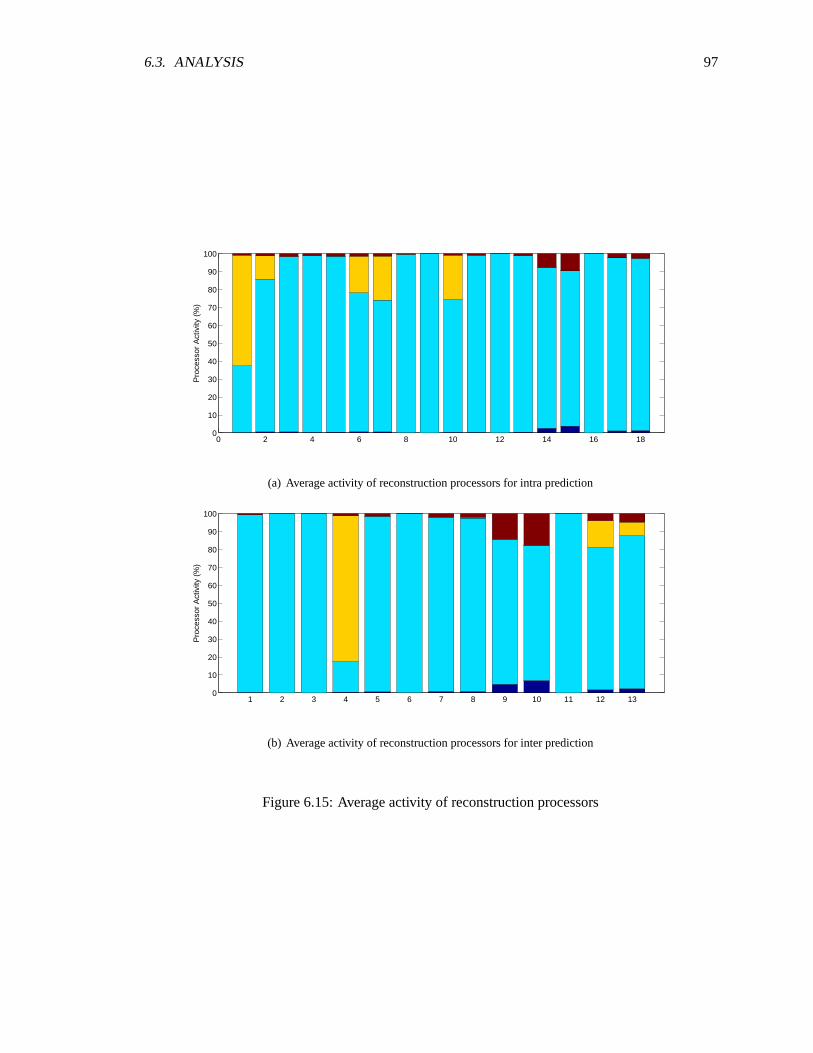
6.3. ANALYSIS 97
0 2 4 6 8 10 12 14 16 180
10
20
30
40
50
60
70
80
90
100
Pro
cess
or A
ctiv
ity (
%)
(a) Average activity of reconstruction processors for intra prediction
1 2 3 4 5 6 7 8 9 10 11 12 130
10
20
30
40
50
60
70
80
90
100
Pro
cess
or A
ctiv
ity (
%)
(b) Average activity of reconstruction processors for inter prediction
Figure 6.15: Average activity of reconstruction processors

98 CHAPTER 6. RESULTS AND ANALYSIS
1 2 3 4 5 6 7 8 9 10 11 12 13 140
10
20
30
40
50
60
70
80
90
100
Pro
cess
or A
ctiv
ity (
%)
(a) Average activity of integer transform processors for intra prediction
1 2 3 4 5 6 7 8 9 10 110
10
20
30
40
50
60
70
80
90
100
Pro
cess
or A
ctiv
ity (
%)
(b) Average activity of integer transform processors for inter prediction
Figure 6.16: Average activity of integer transorm processors
are bottle necks using the majority of encoding time.
Optimization
Because of the low activity of the processors, the majority of power is wasted on cycling
on empty cycles. For the power optimization the voltage and frequency of each processor can be
scaled for efficiency. Original measurements are taken with the chip running at full power at 1.3V
and 1.2 GHz, using this activity number, the frequency is scaled for each processors for greater
utilization. Reducing the frequency by a factor of 2 increases the activity of that processors by a
factor of 2. To achieve maximum efficiency the frequency can be scaled by any multiple, in this
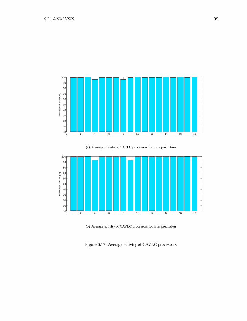
6.3. ANALYSIS 99
0 2 4 6 8 10 12 14 16 180
10
20
30
40
50
60
70
80
90
100
Pro
cess
or A
ctiv
ity (
%)
(a) Average activity of CAVLC processors for intra prediction
0 2 4 6 8 10 12 14 16 180
10
20
30
40
50
60
70
80
90
100
Pro
cess
or A
ctiv
ity (
%)
(b) Average activity of CAVLC processors for inter prediction
Figure 6.17: Average activity of CAVLC processors
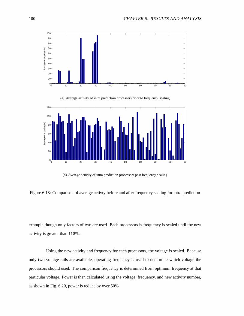
100 CHAPTER 6. RESULTS AND ANALYSIS
0 10 20 30 40 50 60 70 80 900
10
20
30
40
50
60
70
80
90
100
Pro
cess
or A
ctiv
ity (
%)
(a) Average activity of intra prediction processors prior to frequencyscaling
0 10 20 30 40 50 60 70 80 900
20
40
60
80
100
120
Pro
cess
or A
ctiv
ity (
%)
(b) Average activity of intra prediction processors post frequency scaling
Figure 6.18: Comparison of average activty before and after frequency scaling for intra prediction
example though only factors of two are used. Each processors is frequency is scaled until the new
activity is greater than 110%.
Using the new activity and frequency for each processors, the voltageis scaled. Because
only two voltage rails are available, operating frequency is used to determinewhich voltage the
processors should used. The comparison frequency is determined from optimum frequency at that
particular voltage. Power is then calculated using the voltage, frequency,and new activity number,
as shown in Fig. 6.20, power is reduce by over 50%.
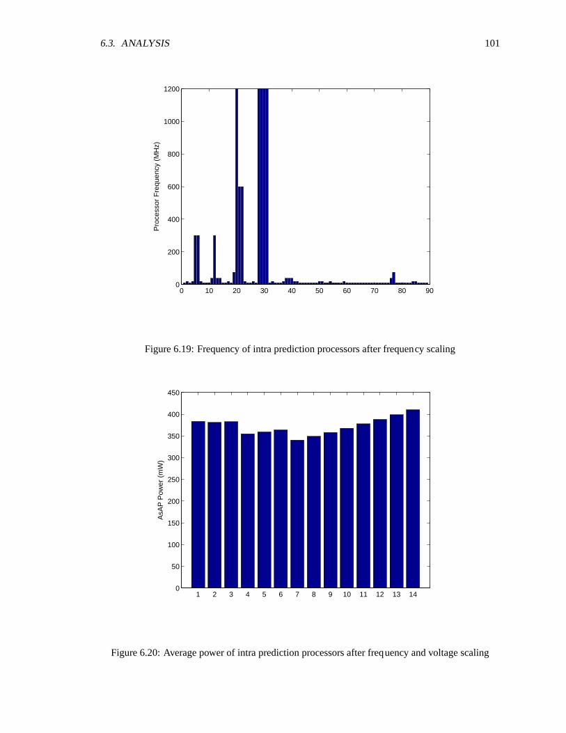
6.3. ANALYSIS 101
0 10 20 30 40 50 60 70 80 900
200
400
600
800
1000
1200
Pro
cess
or F
requ
ency
(M
Hz)
Figure 6.19: Frequency of intra prediction processors after frequency scaling
1 2 3 4 5 6 7 8 9 10 11 12 13 140
50
100
150
200
250
300
350
400
450
AsA
P P
ower
(m
W)
Figure 6.20: Average power of intra prediction processors after frequency and voltage scaling

102 CHAPTER 6. RESULTS AND ANALYSIS
0 10 20 30 40 50 60 70 800
10
20
30
40
50
60
Pro
cess
or A
ctiv
ity (
%)
(a) Average activity of inter prediction processors prior to frequencyscaling
0 10 20 30 40 50 60 70 800
20
40
60
80
100
120
Pro
cess
or A
ctiv
ity (
%)
(b) Average activity of inter prediction processors post frequency scaling
Figure 6.21: Comparison of average activity before and after frequency scaling for inter prediction
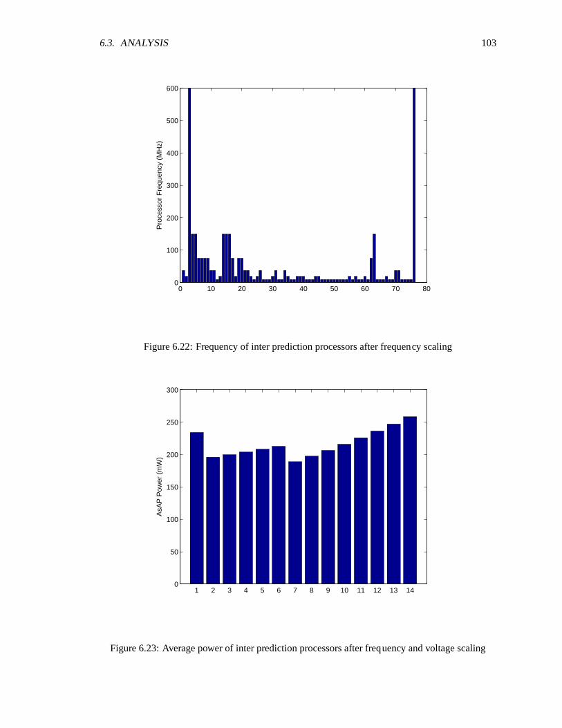
6.3. ANALYSIS 103
0 10 20 30 40 50 60 70 800
100
200
300
400
500
600
Pro
cess
or F
requ
ency
(M
Hz)
Figure 6.22: Frequency of inter prediction processors after frequency scaling
1 2 3 4 5 6 7 8 9 10 11 12 13 140
50
100
150
200
250
300
AsA
P P
ower
(m
W)
Figure 6.23: Average power of inter prediction processors after frequency and voltage scaling

104 CHAPTER 6. RESULTS AND ANALYSIS
6.3.4 Processor Memory Usage
This section presents the instruction data memory usage of the all the processors. The
majority of the processors average around 45 instructions and the main computation processors av-
eraging around 100 instructions. A greater instruction memory block would reduce the number of
processors required and increase the percentage of time that each computation processor is active,
however much of this space might not be used because nearly half the processors are used for routing
and memory purposes. Increasing the amount of code in each processors may also decrease through-
put due to less parallelization, but would also reduce the overhead of code splitting. Many of the
processors in intra prediction if further divided would not provide any additional speed up through
parallelization because of data dependencies. The dynamically configurable memory (DCMem)
count is only given for memory processors where they are used for computation, DCMem registers
that are used for setting output directions and long distance communication are not used.
The instruction count spread for integer transform and CAVLC are fairly constant because
the majority of processors are used for computation and few routing processors are needed. These
processes are also done on a 4x4 block basis only so the amount of control can also be reduced
because data can be stored locally and passed along at every stage. Inthe CAVLC even less variables
are needed for the actual computation but the majority of the instruction memory is used for storing
look-up tables and checking previous encoding levels.
6.3.5 Communication
This section looks at the communication links used the AsAP processors. Each link is
assigned a number for reference only, this does not correlate with any modules or functions. Link
length is measured by the number of processors between the beginning andend minus 1, so a link
between two neighboring processors would have a length of one. The average number of cycles
between writes is taken from beginning of simulation (after configuration) till the end of simulation
and is used to calculate the average throughput. These throughput values are calculated based on a
simulation running at 1.3V and 1.22 GHz. Max throughput is calculated from the average number
of cycles between writes when stalling time is not included. These max values are much greater
than the average throughput giving the approximate throughput when active. Two tables are given,

6.3. ANALYSIS 105
Processor I m e m D m e m D C M e m Processor I m e m D m e m D C M e mdata collector 46 6 - reorder resdu 2 35 128 7
main control 82 9 - QP table 46 118 -
redirect 38 5 - 4x4 transform 117 32 -
MB request 17 0 - 4x4 AC 1 44 75 -
intra control 95 7 - 4x4 AC 2 62 74 -
intra Cb/Cr mem 60 128 7 2x2 DC transform 85 70 -
intra Y mem 1 42 128 5 2x2 quantization 118 58 -
intra Y mem 2 47 128 5 16x16 DC transform 78 40 -
intra mem control 13 1 - 16x16 quantization 31 51 -
16x16 DC 117 78 - zig zag 2 83 40 -
16x16 resdu 70 128 7 temp hold 6 128 3
16x16 resdu 2 97 128 18 CAVLC scan 2 69 50 -
router 14 3 - data receiver 103 10 -
router 37 5 - luma nnz 2 72 24 -
reorder resdu 49 28 - luma nnz 1 127 48 -
intra resdu 31 128 8 Cb/Cr nnz 110 44 -
intra resdu 2 37 128 7 zig zag 1 79 35 -
test generator 113 89 - CAVLC scan 1 98 50 -
transform generator 37 9 - num coeff 75 119 -
16x16 H/V 127 51 - sign trailing 1's 115 89 -
4x4 DC pred 118 47 - router 21 10 -
4x4 DC resdu 102 49 - level code 1 71 50 -
4x4 vertical 116 55 - level code 2 121 44 -
4x4 horizontal 103 55 - total zero 56 124 -
router 15 3 - router 13 3 -
MB reconstruction 14 3 - non zero run 46 62 -
16x16 pred 1 40 128 5 router 25 5 -
16x16 pred 2 22 128 2 CAVLC out 44 14 -
4x4 pred 1 111 128 4 SPS/PPS 50 25 -
4x4 pred 2 92 128 4 SH 126 10 -
pred. collector 34 5 - intra pred mode 63 45 -
DC pred 24 18 - inter mv mode 90 45 -
vertical pred 22 18 - router 11 5 -
horizontal pred 17 18 - output 81 22 -
4x4 resdu 19 6 - inter control 115 25 -
Cb/Cr resdu 27 128 5 ME\_ACC control 106 40 -
router 21 1 - calc SAD 58 15 -
router 26 2 - calc MV 121 24 -
router 14 0 - calc MV mem control 38 20 -
router 17 0 - ref Y 0 45 128 5
router 18 1 - ref Y 1 46 128 5
router 26 1 - ref Y 2 46 128 5
router 18 1 - ref Y 3 46 128 5
router 15 0 - ref Y 4 46 128 5
router 16 3 - ref Y 5 46 128 5
chroma pred 41 128 2 ref Y 6 46 128 5
Cb/Cr H/V 127 59 - ref Y 7 46 128 5
Cb/Cr DC 112 62 - ref Y 8 46 128 5
Cb/Cr DC 2 121 54 - cur Y 46 128 5
16x16 dequant 77 50 - ref C 0 41 128 5
2x2 dequant 58 24 - ref C 1 41 128 5
AC rescale 94 65 - ref C 2 41 128 5
router 23 9 - ref C 3 41 128 5
router 19 2 - ref C 4 35 128 5
inverse transform 79 44 - calc inter MB 72 12 -
reorder 46 28 - inter resdu calc 124 10 -
reorder resdu 1 36 128 8
Figure 6.24: Number of instruction and data memory words used per processors. Dynamic Mem-ory (DC Mem) is only listed for memory processors where they are used fordata storage andcomputation.

106 CHAPTER 6. RESULTS AND ANALYSIS
02 04 06 08 01 0 01 2 01 4 0N umb erof I nst ructi onsper P rocessor
Figure 6.25: Number of instruction memory words used per processor
02 04 06 08 01 0 01 2 01 4 0N umb erofI nst ructi onsperP rocessor
(a) Number of instruction memory words for intra prediction
processors
02 04 06 08 01 0 01 2 01 4 0N umb erofI nst ructi onsperP rocessor
(b) Number of instruction memory words for inter prediction
processors
Figure 6.26: Instruction memory usage for prediction processors
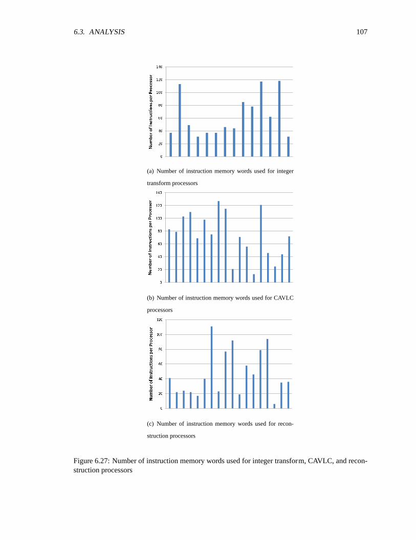
6.3. ANALYSIS 107
02 04 06 08 01 0 01 2 01 4 0N umb erofI nst ructi onsperP rocessor
(a) Number of instruction memory words used for integer
transform processors
02 04 06 08 01 0 01 2 01 4 0N umb erofI nst ructi onsperP rocessor
(b) Number of instruction memory words used for CAVLC
processors
02 04 06 08 01 0 01 2 0N umb erofI nst ructi onsperP rocessor
(c) Number of instruction memory words used for recon-
struction processors
Figure 6.27: Number of instruction memory words used for integer transform, CAVLC, and recon-struction processors
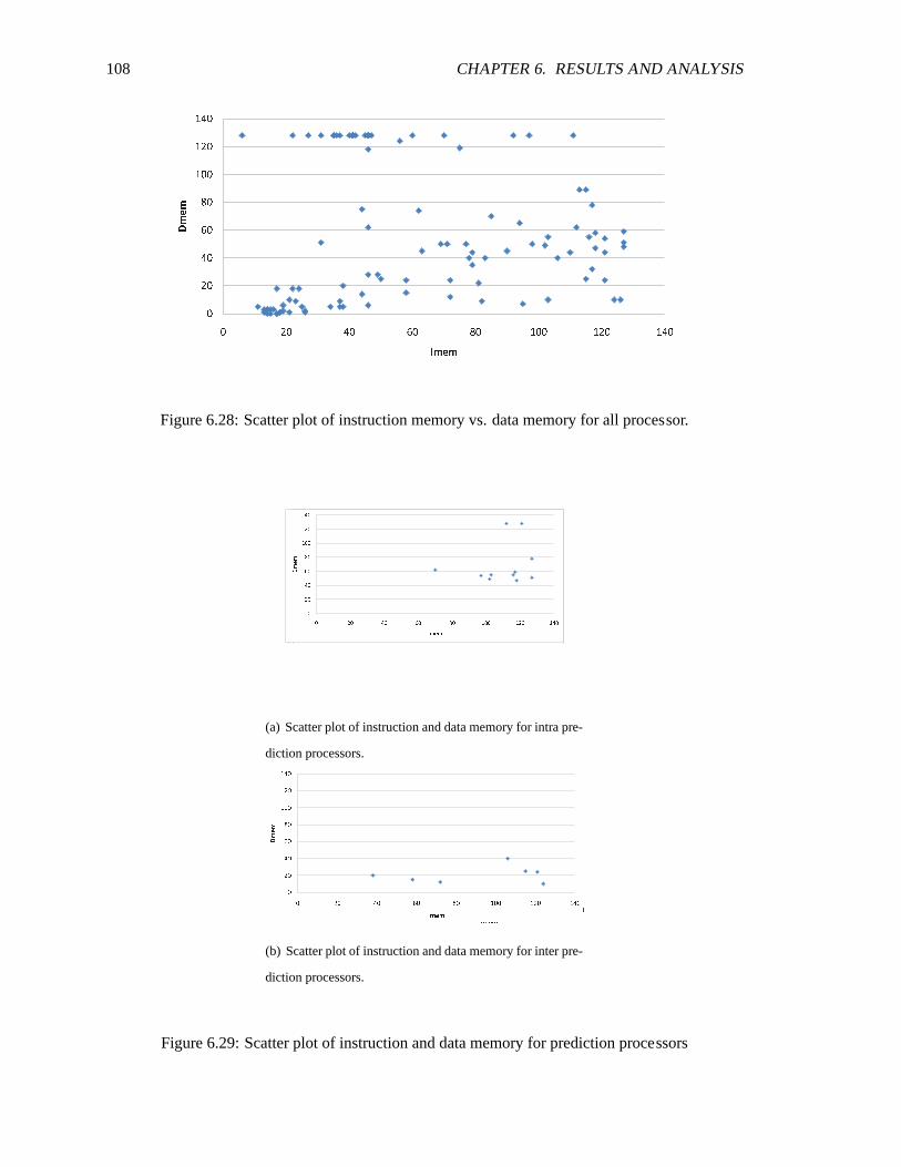
108 CHAPTER 6. RESULTS AND ANALYSIS
02 04 06 08 01 0 01 2 01 4 0
0 2 0 4 0 6 0 8 0 1 0 0 1 2 0 1 4 0D mem
I m e mFigure 6.28: Scatter plot of instruction memory vs. data memory for all processor.
02 04 06 08 01 0 01 2 01 4 00 2 0 4 0 6 0 8 0 1 0 0 1 2 0 1 4 0D mem I m e m02 04 06 08 01 0 01 2 01 4 0
0 2 0 4 0 6 0 8 0 1 0 0 1 2 0 1 4 0D mem I m e mD C T
02 04 06 08 01 0 01 2 01 4 00 2 0 4 0 6 0 8 0 1 0 0 1 2 0 1 4 0D mem I m e m
C A V L C02 04 06 08 01 0 01 2 01 4 0
0 2 0 4 0 6 0 8 0 1 0 0 1 2 0 1 4 0D mem I m e m(a) Scatter plot of instruction and data memory for intra pre-
diction processors.
2 0 4 0 6 0 8 0 1 0 0 1 2 0 1 4 0I m e mI n t r a P r e d
02 04 06 08 01 0 01 2 01 4 00 2 0 4 0 6 0 8 0 1 0 0 1D mem I m e m
C A V L C02 04 06 08 01 0 01 2 01 4 0
0 2 0 4 0 6 0 8 0D mem D C T02 04 06 08 01 0 01 2 01 4 0
0 2 0 4 0 6 0 8 0 1 0 0 1 2 0 1 4 0D mem I m e m(b) Scatter plot of instruction and data memory for inter pre-
diction processors.
Figure 6.29: Scatter plot of instruction and data memory for prediction processors
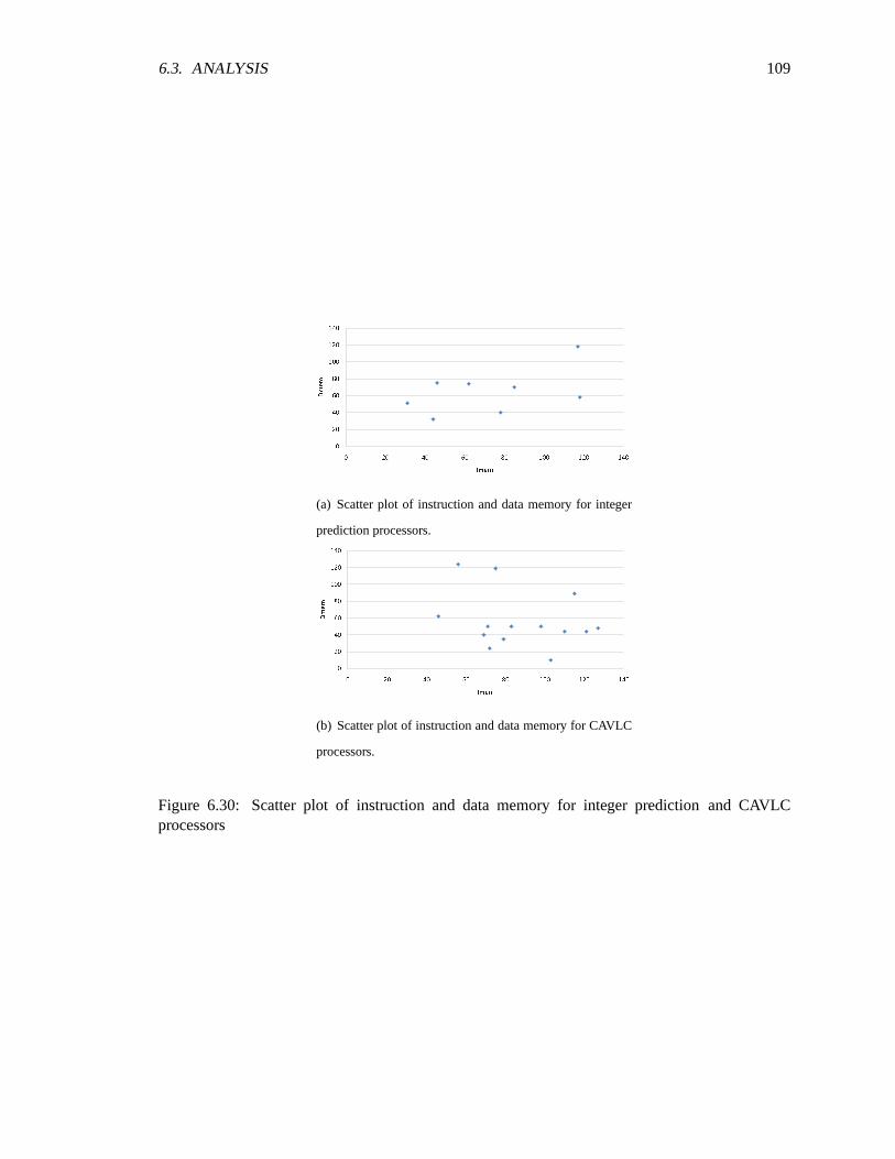
6.3. ANALYSIS 109
02 04 06 08 01 0 01 2 01 4 00 2 0 4 0 6 0 8 0 1 0 0 1 2 0 1 4 0D mem
I m e m02 04 06 08 01 0 01 2 01 4 00 2 0 4 0 6 0 8 0 1 0 0 1 2 0 1 4 0D mem
I m e m(a) Scatter plot of instruction and data memory for integer
prediction processors.
02 04 06 08 01 0 01 2 01 4 00 2 0 4 0 6 0 8 0 1 0 0 1 2 0 1 4 0D mem
I m e m02 04 06 08 01 0 01 2 01 4 00 2 0 4 0 6 0 8 0 1 0 0 1 2 0 1 4 0D mem I m e m
D C T02 04 06 08 01 0 01 2 01 4 0
0 2 0 4 0 6 0 8 0 1 0 0 1 2 0 1 4 0D memI m e m
(b) Scatter plot of instruction and data memory for CAVLC
processors.
Figure 6.30: Scatter plot of instruction and data memory for integer predictionand CAVLCprocessors

110 CHAPTER 6. RESULTS AND ANALYSISP r o c e s s o r L e n g t h A v e r a g e M a x P r o c e s s o r L e n g t h A v e r a g e M a xT h r o u g h p u t T h r o u g h t p u t T h r o u g h p u t T h r o u g h t p u t data collector 1 0.241 7.6 zig zag 2 1 12 505
main control 1 33.2 809.3 zig zag 1 1 12 510
main control 1 0.103 1.9 CAVLC data receiver 1 13.1 1200
MB request 1 0.0685 0.0695 CAVLC data receiver 1 0.37 52.1
redirect 1 64.3 186700 CAVLC data receiver 2 12.8 1200
intra control 1 6.6 105.1 Cb/Cr pred nnz 1 0.705 100
intra control 4 813 813 CAVLC scan 2 1 3.8 180
intra control 9 2.2 37.9 CAVLC scan 2 2 6.5 314
intra control 3 0.103 2.2 CAVLC scan 1 1 7.4 316
intra control 1 2.2 37.9 CAVLC scan 1 3 2.1 88.9
intra mem Y 1 1 813 154900 CAVLC scan 1 1 3.9 165.2
intra mem Y 2 1 98.2 98.6 num coeff 1 4.5 430.6
test generator 9 0.236 47.3 luma pred nnz 2 2 5.1 544
16x16 DC 1 14.8 109.1 luma pred nnz 1 2 0.994 65
16x16 DC 1 0.45 4.7 luma pred nnz 1 1 0.994 65
16x16 H/V 1 2 16.1 SPS/PPS 1 1.2 1200
Tx start 1 24.5 98600 sign 1's 1 9 449
Cb/Cr DC 1 8.3 117.6 sign 1's 2 7.4 368
QP table 1 24.3 1600 sign 1's 1 3.1 151
QP table 1 0.236 24.9 router 1 7.5 7000
4x4 AC 1 6 12.4 472.8 level code 1 1 8.5 393
4x4 AC 1 1 13 510 SH 1 2000 5200
2x2 DC HT 1 12.1 2200 intra mode pred 1 143.7 2300
2x2 DC HT 1 0.236 62.9 Inverse Tx reorder 1 8.2 443
reorder Cb/Cr 9 5.1 1600 AC rescale 3 0.0337 0.207
4x4 DC pred 1 0.74 11.6 total zero 1 7.4 699
4x4 DC pred 1 2.4 37.1 total zero 2 3.1 250
4x4 horizontal 1 4.7 32 router 1 8.1 1200
4x4 horizontal 1 0.461 3.3 level code 2 1 6.7 484
4x4 Tx 1 11.8 274.1 router 1 4.6 1300
4x4 Tx 2 12.3 284 MV pred 1 6200 17100
4x4 AC 2 6 11.6 485 non zero run 2 7.4 420
4x4 AC 2 1 11.5 482 router 1 15.7 3900
2x2 quant 1 23.2 3500 CAVLC out 11 18.3 1700
2x2 quant 5 0.498 67.4 output 1 13.4 1400
Figure 6.31: Average and max throughput of major intra prediction communication links. Linklenght is determined by the number of intersected processros minus 1.
one for intra and one for inter prediction.

6.3. ANALYSIS 111
P r o c e s s o r L e n g t h A v e r a g e M a x P r o c e s s o r L e n g t h A v e r a g e M a xT h r o u g h p u t T h r o u g h t p u t T h r o u g h p u t T h r o u g h t p u tdata collector 1 1.1 6.4 2x2 DC HT 1 0.193 35.8
main control 1 216 8900 4x4 Tx 1 10.7 276.3
main control 1 0.534 23.1 4x4 Tx 2 10.4 272.6
MB request 1 1.4 1.4 4x4 AC 2 1 10.3 465
ref Y 2 1 13.7 62.3 4x4 AC 2 6 10.3 465
ref Y 3 1 13.7 66.2 2x2 quant 1 20.7 2600
ref Y 6 1 13.7 81.7 2x2 quant 6 0.455 63.7
ref Y 7 1 13.7 88.6 zig zag 2 1 10.8 482.3
ref Y 8 1 13.7 96.7 zig zag 1 1 10.7 486.6
cur Y 1 13.7 106.6 data receiver 2 11.4 1000
ref C 2 1 13.7 153.4 data receiver 1 0.386 37.8
ref C 3 1 13.7 179.6 data receiver 1 11.4 1000
request MB 9 1.4 2500 Cb/Cr pred nnz 1 0.649 99.6
redirect 1 215.3 9300 CAVLC scan 2 1 3.3 185.4
ref Y 0 1 13.7 59.1 CAVLC scan 2 2 4.6 257.5
ref Y 0 1 18.5 61.4 CAVLC 1 5.4 261.7
ref Y 1 1 13.7 59.8 CAVLC 3 1.9 93.6
ref Y 4 1 13.7 70.7 CAVLC scan 1 1 3.5 172.3
ref Y 5 1 13.7 75.8 num coeff 1 4.1 415.1
router 1 0.338 15.1 luma pred nnz 2 2 4.3 511.8
ref C 0 1 13.7 118.6 luma pred nnz 1 2 0.853 63.6
ref C 1 1 13.7 133.8 luma pred nnz 1 1 0.853 63.6
ref C 4 1 13.7 211.6 SPS/PPS 1 1.1 719
inter control 2 0.241 4.3 sign 1's 1 6.8 444.3
inter control 1 0.265 4.8 sign 1's 2 5.4 352.1
inter control 1 133 3000 sign 1's 1 2.8 183
router 1 0.289 10.8 router 1 6.8 4100
test generator 8 0.434 54.1 level code 1 1 6.3 369.1
test generator 3 0.048 6 SH 1 2.7 4200
calc. resdu 9 13.7 389.1 resdu reorder 2 8.5 306
calc SAD 1 0.193 2.7 AC rescale 3 0.048 0.207
calc SAD 6 0.241 3.4 total zero 1 5.4 531
ME control 2 3.6 391.7 total zero 2 2.8 275.4
ME control 1 0.526 58 router 1 6.4 987.2
calc MV 17 0.193 1600 level code 2 1 2.1 440.6
Integer Start 1 20.5 8800 router 1 4.5 1100
QP table 1 20.6 1400 inter mv pred 1 0.338 399
QP table 1 0.338 24.9 non zero run 2 4.5 438
4x4 AC 6 11 455.8 router 1 13.1 2700
4x4 AC 1 11.8 488.6 CAVLC out 11 13.5 1300
2x2 DC HT 1 10.7 1800 output 1 15.8 1300
Figure 6.32: Average and max throughput of major inter prediction communication links. Linklength is determined by the number of intersected processors minus 1.

112 CHAPTER 6. RESULTS AND ANALYSIS

113
Chapter 7
Future Work and Conclusion
7.1 Architecture Enhancements for Parallel Programming
This implementation of the H.264 encoder has been highly parallelized for maximum
performance, however many of the techniques used are due to limitation in the processing platform,
some enhancements are suggested for improving the parallel programming process and increasing
performance.
7.1.1 Multiple I/O Chips
The small and simple processor architecture of AsAP allows for the easy replication of
many cores and low power advantages. Larger programs will be bound by memory issues however
and having multiple I/O ports for the chip will give much needed bandwidth and reduce extra control
logic that was added to support dual output functions as well as long distance communication.
Multiple I/O ports would also allow for multiple applications to run simultaneously.
7.1.2 Multiple Input Processors
As shown in the analysis, the majority of power is consumed through routing processors,
this was necessary because only two inputs were available per processor and could not be dynam-
ically configured. Increasing the number of inputs per processor wouldgreatly reduce the number
of processors and power needed.
114 CHAPTER 7. FUTURE WORK AND CONCLUSION
7.1.3 Local Shared Memory
Many of the processors are used as shared memory for other processors, these however
only provide small amounts of extra memory and when many are needed the access time is greatly
increased because the data must trickle through all the routing processors. Having small local shared
memories weather dedicated or processor configured would allow for faster throughput and free up
more processors for other tasks.
7.2 Tool Enhancements for Parallel Programming
The majority of time spent in implementing this encoder was in the debug phase, because
of the number of processors used (131) and the simulation time, this proved tobe the most difficult
task.
7.2.1 Arbitrary Mapping Tool For AsAP2
The mapping for this encoder has been hardcoded, using a tool similar to thearbitrary
mapping tool available for MPI-C and AsAP1 would greatly speed up the process and reduce com-
munication connection problems. This would also allow for greater ease in modifying this applica-
tion at a later point.
7.2.2 Analysis of I/O Traffic
One of the most useful debugging tools was to look at the program counterand stall sig-
nals for the input FIFOs and output in ModelSim. A tool that would allow for quick easy viewing
as well as flagging which processor caused the final stall signal (traceback) to occur would greatly
reduce debugging time. Another feature that would be helpful would be to also have a few instruc-
tions in the processor causing the stall available to quick viewing. Often times theerror would be a
simple typo or branch error but would require a lot debugging time to manually do trace back.

7.3. ADDITIONAL ENCODING FUNCTIONS ON ASAP 115
7.2.3 Enhanced I/O File Operations
The H.264 encoder has a feedback loop for storing the reconstructed data, since this is too
large to fit on AsAP, it must be stored off chip. In simulation however this is not possible because
the input file used for reading cannot also be written to in the same instance. Atool that can provide
this function would improve the accuracy of testing and debugging.
7.3 Additional Encoding Functions on AsAP
The encoder presented has been simplified reducing the capabilities and advantages of the
H.264 standard. Future work in these areas would improve the compressionand quality of encoded
videos.
Intra Prediction
In intra prediction, only 3 modes are currently used, by using all available modes in the
standard the entropy values of the encoded bitstream can be reduced. Each prediction mode has
been implemented on either one or two processors, adding additional modes on separate processors
should be fairly simple, the only problems would be with the shared memory which can be replicated
and mode decision which may need to be done on a separate processor.
Inter Prediction
One the advantages of H.264 over previous standards is the ability to use interpolated
samples. Because of the complexity of the motion estimation process only integer samples were
used in the MEACC. Fully supporting interpolated samples in the future will probably also need to
be done via an accelerator. A possible work around for this would be usea smaller search window
and interpolate the samples outside of the MEACC and send them in as if they were part of the
window used by the accelerator. This process though would like increasethe latency of the encoder
significantly.

116 CHAPTER 7. FUTURE WORK AND CONCLUSION
Encoding With Slices
The H.264 standard also supports encoding using slices. The advantageof this is that
each slice of the picture/frame can be encoded independently (using data for previous matching
slices only). On AsAP these can be done in parallel increasing the throughput, the only limitation
would then be in hardware where each module would need to be replicated.
Support for HD-resolution
The algorithm presented can be optimized to support up to 720p real time or nearly 1080p-
resolution (20fps) when using inter prediction. Initial calculations for this are based off the number
of macroblocks that can be loaded for the MEACC within a second. The current implementation
loads 10 macroblocks every time, this can be reduced to 4 macroblocks by re-using the previously
loaded ones however the control logic becomes more complicated since the reference blocks must
be stored in processors for residue calculation and do not provide foreasy indexing.
7.4 Conclusion
Here an H.264 compliant baseline encoder has been implemented in both MPI and on a
programmable parallel processor. The AsAP implementation is shown to be comparable in perfor-
mance to other DSP while achieving the low power capabilities of ASICs. An analysis of perfor-
mance and chip usage is also given to provide a stepping stone for future programs and architectures
in parallel processing. In applications such as this, the primary source ofpower consumption are
from the ME ACC and the shared memories, optimizing code for the computation processors will
not provide any significant reduction in power will only provide more speed. A more practical ap-
proach towards power might be to not use the MEACC but implement the process using individual
processors, although this is much more complex, there is the possibility of 90% power reduction.
117
Bibliography
[1] Iain E. G. Richardson.H.264 adn MPEG-4 Video Compression Video Coding for Next gener-ation Multimedia. John Wiley Sons Ltd, 2003.
[2] International Standard Organization and Information Technology-Coding of Audio-Visual Ob-jects.Part10-Advanced Video Coding. ISO/IEC 14496-10.
[3] Z. Xiao and B. M. Baas. A high-performance parallel CAVLC encoder on a fine-grainedmany-core system. InIEEE International Conference of Computer Design (ICCD), October2008.
[4] Yen-Kuang Chen, Eric Q. Li, Xiaosong Zhou, and Steven Ge. Implementation of h.264 en-coder and decoder on personal computers.Journal of Visual Communication and Image Rep-resentation, 2006.
[5] Zhenyu Wei, Kai Lam Tang, and King N. Ngan. Implementation of h.264 on mobile devices.In IEEE Transactions on Consumer Electronics, 2007.
[6] Yu-Wen Huang et al. A 1.3 tops h.264/avc single-chip encoder for hdtv applications. InISSCCConference on Multimedia Processing, 2005.
[7] D. Truong, W. Cheng, T. Mohsenin, Z. Yu, T. Jacobson, G. Landge, M. Meeuwsen, C. Watnik,P. Mejia, A. Tran, J. Webb, E. Work, Z. Xiao, and B. Baas. A 167-processor 65 nm com-putational platform with per-processor dynamic supply voltage and dynamicclock frequencyscaling. InSymposium on VLSI Circuits, pages 22–23, June 2008.
[8] R. W. Apperson, Z. Yu, M. J. Meeuwsen, T. Mohsenin, and B. M.Baas. A scalable dual-clockFIFO for data transfers between arbitrary and haltable clock domains.IEEE Transactions onVery Large Scale Integration (VLSI) Systems, 15(10):1125–1134, October 2007.
[9] W. H. Cheng and B. M. Baas. Dynamic voltage and frequency scaling circuits with twosupply voltages. InIEEE International Symposium on Circuits and Systems (ISCAS), pages1236–1239, May 2008.
[10] Michael Meeuwsen, Zhiyi Yu, and Bevan M. Baas. A shared memory module for asyn-chronous arrays of processors. 2007.
[11] Gouri Landge. A configurable motion estimation accelerator for videocompression. Master’sthesis, University of California Davis, 2009.
[12] Eric W. Work. Algorithms and software tools for mapping arbitrarily connected tasks ontoan asynchronous array of simple processors. Master’s thesis, University of California, Davis,CA, USA, September 2007.http://www.ece.ucdavis.edu/vcl/pubs/theses/2007-4.

118 BIBLIOGRAPHY
[13] Kun Ouyang, Qing Ouyang, and Zhengda Zhou. Optimization and implementation of h.264encoder on symmetric multi-processor platform. In2009 WRI World Congress on ComputerScience and Information Engineering, pages 265–269, 2009.
[14] G Nageswara Rao, D Jaya Chandra Prasad RSV, and Srividya Narayanan. Real-time softwareimplementation of h.264 baseline profile video encoder for mobile and handhelddevices. InIEEE International Conference on Acoustics, Speech and Signal Processing, 2006, 2006.
[15] Tung-Chien Chen et al. Analysis and architecture design of an hdtv720p 30 frames/s h.264/avcencoder.IEEE Transactions on Circuits and Systems for Video Technology, 2006.