Loughborough UniversityInstitutional Repository

A fault tree analysis strategyusing binary decision

diagrams

This item was submitted to Loughborough University's Institutional Repositoryby the/an author.

Additional Information:

• This pre-print has been submitted, and accepted, to the journal, Re-liability Engineering and System Safety [ c© Elsevier]. The defini-tive version: REAY, K.A. and ANDREWS, J.D., 2002. A Faulttree analysis strategy using binary decision diagrams. ReliabilityEngineering and System Safety, 78(1), pp.45-56, is available at:http://www.sciencedirect.com/science/journal/09518320.

Metadata Record: https://dspace.lboro.ac.uk/2134/442

Please cite the published version.

1

A Fault Tree Analysis Strategy Using Binary Decision Diagrams.

Karen A. Reay and John D. Andrews

Loughborough University, Loughborough, Leicestershire, LE11 3TU.

Abstract

The use of Binary Decision Diagrams (BDDs) in fault tree analysis provides both an accurate

and efficient means of analysing a system. There is a problem however, with the conversion

process of the fault tree to the BDD. The variable ordering scheme chosen for the

construction of the BDD has a crucial effect on its resulting size and previous research has

failed to identify any scheme that is capable of producing BDDs for all fault trees. This paper

proposes an analysis strategy aimed at increasing the likelihood of obtaining a BDD for any

given fault tree, by ensuring the associated calculations are as efficient as possible. The

method implements simplification techniques, which are applied to the fault tree to obtain a

set of 'minimal' subtrees, equivalent to the original fault tree structure. BDDs are constructed

for each, using ordering schemes most suited to their particular characteristics. Quantitative

analysis is performed simultaneously on the set of BDDs to obtain the top event probability,

the system unconditional failure intensity and the criticality of the basic events.

1. Introduction

The Binary Decision Diagram (BDD) method(1) has emerged as an alternative to conventional

techniques for performing both qualitative and quantitative analysis of fault trees. BDD's are

already proving to be of considerable use in reliability analysis, providing a more efficient

means of analysing a system, without the need for the approximations previously used in the

traditional approach of Kinetic Tree Theory(2).

The BDD method does not analyse the fault tree directly, but converts the tree to a binary

decision diagram, which represents the Boolean equation for the top event. The difficulty,

however, lies with the conversion of the tree to the BDD. An ordering of the fault tree

variables (basic events) must be chosen and this ordering can have a crucial effect on the

size of the resulting BDD; it can mean the difference between a minimal BDD with few nodes,

providing an efficient analysis and being able to produce any BDD at all. There is no universal

ordering scheme that can be successfully used to produce a minimal BDD for all fault trees;

indeed no scheme has been found that will produce a BDD (minimal or otherwise) for some

large fault trees. Emphasis in the research has now turned to applying alternative techniques

that will increase the likelihood of obtaining a BDD for any given fault tree, by ensuring the

associated calculations are as efficient as possible.

2

In this paper, an analysis strategy is proposed which implements these requirements. The

initial stage combines two simplification techniques that have been shown to be

advantageous in the construction of BDDs: Faunet reduction(3), and linear-time

modularisation(4). The reduction technique reduces the fault tree to its minimal logic form,

whilst modularisation identifies independent subtrees (modules) existing within the tree that

can be analysed separately. This results in a set of 'minimal' fault trees, equivalent to the

original fault tree structure.

A neural network is used to select the most appropriate ordering scheme(5,6) for each

independent module of the fault tree, based upon its individual characteristics. BDDs are

obtained for each module in separate computations, culminating in a set of BDDs, which

together represent the original system.

Quantitative analysis is performed simultaneously on the set of BDDs to obtain the top event

probability, the system unconditional failure intensity and the criticality of the basic events.

Each of these stages is described in more detail in the following sections and demonstrated

throughout with the use of an example fault tree.

2. Simplification of the Fault Tree Structure

Two pre-processing techniques are applied to the fault tree in order to obtain the smallest

possible subtrees, so that the process of constructing the BDDs becomes simple and

efficient. The first stage of pre-processing is Faunet reduction, a technique that is used to

restructure the fault tree to its most concise form. Once this has been applied however, it is

possible to simplify the analysis further by identifying independent subtrees (modules) within

the fault tree that can be treated separately. The linear-time algorithm is an extremely efficient

method of modularisation and forms the second stage of the fault tree pre-processing. This

results in a set of independent fault trees each with the simplest possible structure, which

together describe the original system.

2.1 Faunet Reduction

FAUNET reduction is a technique that is used to reduce the fault tree to its minimal form, so

eliminating any ‘noise’ from the system, without altering the underlying logic. Its effectiveness

has been demonstrated with its application to a large set of fault trees, where it decreased the

size of the resulting BDDs by approximately 50%. The method consists of three stages:

• Contraction

Subsequent gates of the same type are contracted to form a single gate. This gives a

fault tree with an alternating sequence of AND gates and OR gates.

3

• Factorisation

Pairs of events that always occur together in the same gate type are identified. They are

combined to form a single complex event, which are given a numerical label from 2000

upwards.

• Extraction

The following two structures are identified and replaced:

Figure 1: The extraction procedure

The above three steps are repeated until no further changes are possible in the fault tree,

resulting in a more compact representation of the system.

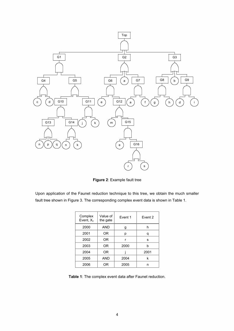
For example, consider the fault tree illustrated in Figure 2.

restructure

restructure

X1 X3X1X2

X1

X3X2

X1

X3X2X1 X3X1X2

4

Figure 2: Example fault tree

Upon application of the Faunet reduction technique to this tree, we obtain the much smaller

fault tree shown in Figure 3. The corresponding complex event data is shown in Table 1.

ComplexEvent, Xc

Value ofthe gate

Event 1 Event 2

2000 AND g h

2001 OR p q

2002 OR r s

2003 OR 2000 b

2004 OR j 2001

2005 AND 2004 k

2006 OR 2005 n

Table 1: The complex event data after Faunet reduction.

Top

G2G1

c

j k

G7

G3

G13

n q

a

p

G5G4

d G11G10

G14

n k

G6

e G12

m G15

e G16

r s

G9bG8

g d ihfa

5

Figure 3: The resulting fault tree after the application of Faunet reduction

Having reduced the fault tree to a more concise form, we now consider the second pre-

processing technique of modularisation.

2.2 Modularisation

The modularisation procedure does not alter the structure of the tree, but detects modules. A

module of a fault tree is a subtree that is completely independent from the rest of the tree.

That is, it contains no basic events that appear elsewhere in the fault tree. The advantage of

identifying these modules is that each one can be analysed separately from the rest of the

tree. The results from subtrees identified as modules are substituted into the higher-level fault

trees where the modules occur.

Using the linear-time algorithm, the modules can be identified after two depth-first traversals

of the fault tree. The first of these performs a step-by-step traversal recording for each gate

and event, the step number at the first, second and final visits to that node. The step number

of the second visit to each event is always equivalent to the step number of the first visit to

that event. To demonstrate this, refer to the fault tree in Figure 3. Starting at the top event and

progressing through the tree in a depth-first manner (and considering the event inputs to a

gate before any gate inputs), the gates and events are visited in the order shown in Table 2.

Each gate is visited at least twice: once on the way down the tree and again on the way back

Top

G2

G7

G32006

aG6

e G12

m G15

2002 e

G92003

d ifa

c

G4

d

6

up the tree. Once a gate has been visited, it can be visited again, but the depth-first traversal

beneath that gate is not repeated. The step numbers of the visits to the gates and events are

shown in Tables 3 and 4.

Step number 1 2 3 4 5 6 7 8 9 10 11

Node Top 2006 G2 a G6 e G12 m G15 2002 e

Step number 12 13 14 15 16 17 18 19 20 21 22

Node G15 G12 G6 G7 a f G7 G2 G3 2003 G9

Step number 23 24 25 26 27 28 29 30 31

Node d i G9 G3 G4 c d G4 Top

Table 2: Order in which the gates and events are visited in the depth-first traversal of the

fault tree in Figure 3.

The second pass through the tree finds the maximum (Max) of the last visits and the minimum

(Min) of the first visits of the descendants (any gates and events appearing below that gate in

the tree) of each gate; these values are shown in Table 3.

Gate Top G2 G3 G4 G6 G7 G9 G12 G15

Visit 1 1 3 20 27 5 15 22 7 9

Visit 2 31 19 26 30 14 18 25 13 12

Last visit 31 19 26 30 14 18 25 13 12

Min 2 4 21 23 6 4 23 6 6

Max 30 18 29 29 13 17 29 12 11

Table 3: Data for the fault tree gates.

Event a c d e f i m 2002 2003 2006

Visit 1 4 28 23 6 17 24 8 10 21 2

Visit 2 4 28 23 6 17 24 8 10 21 2

Last visit 16 28 29 11 17 24 8 10 21 2

Table 4: Data for the fault tree events.

The principle of the algorithm is that if any descendant of a gate has a first visit step number

smaller than the first visit step number of the gate, then it must also occur beneath another

gate. Conversely, if any descendant has a last visit step number greater than the second visit

step number of the gate, then again it must occur elsewhere in the tree. Therefore, a gate can

be identified as heading a module only if:

7

• The first visit to each descendant is after the first visit to the gate

and

• The last visit to each descendant is before the second visit to the gate

Therefore, the following gates can be identified as modules:

Top, G2 and G6

For completeness, the top event (Top) is included in this list, even though it will always be a

module of the fault tree.

The occurrences of these subtrees are replaced by the single modular events, which are

named in the same way as complex events (i.e. they take on the next available value above

2000).

Top - 2007, G2 - 2008, G6 - 2009

Three separate fault trees as shown in Figure 4 now replace the fault tree in Figure 3.

(a) - Module 2007 (b) - Module 2008 (c) - Module 2009

Figure 4: The three modules obtained from the fault tree shown in Figure 3

Having reduced the fault tree to its minimal form and identified all the independent modules,

the pre-processing of the fault tree is complete and the next step is to obtain the associated

BDDs.

3. Obtaining the Associated Binary Decision Diagrams

A BDD must be constructed for each of the modules. As they all have different properties,

using the same variable ordering scheme for each may not be appropriate. Therefore an

ordering scheme is selected for each module based on its unique characteristics through the

Top

c

G3 2006 G4

dG92003

d i

2008

G6

e G12

m G15

e 2002

G2

G7a

fa

2009

8

use of a pre-programmed neural network. The neural network selects the best ordering

scheme from eight possible alternatives, which include both structural and weighted schemes.

The BDD for each module is then obtained using the variable ordering determined by the

appropriate scheme.

Considering the module '2007' in Figure 4(a), the modified priority depth-first scheme (a

depth-first left-right exploration, considering the most repeated events under any gate first and

considering gates with only event inputs before any others) was identified as the most

suitable by the neural network. This gives the following ordering:

2008 < 2006 < d < c < 2003 < i

The BDD obtained using this ordering is shown in Figure 5. It is known as the 'primary' BDD,

as it represents the top event and is used to calculate the system unavailability.

Figure 5: The primary BDD (module '2007') obtained from the ordering

2008<2006<d<c<2003<i

Each module is treated in the same manner, with its BDD nodes labelled consecutively from

the one previously constructed in order to avoid confusion.

The BDDs were constructed for the two remaining modules in the example. The modified

depth-first scheme (a depth-first left-right exploration, considering the most repeated events

under any gate first) was used for module '2008', producing the ordering:

a<2009<f

2003

2006

d

2003

c

0

1

0

0

11

2008

i

0

0

F1

F7F6

F5F4

F3

F2

9

m

e

0

1

1

2002

0

F10

F12

F11

a

1

1

2009

0

F9

F8

The modified top-down scheme (a left-right, top-down exploration of the tree, considering

repeated events first) was used for module '2009' giving:

e<m<2002

The resulting BDDs, which also illustrate the node labelling, are shown in Figure 6.

(a) - BDD for module '2008' (b) BDD for module '2009'

Figure 6: The BDDs for modules '2008' and '2009', demonstrating node labelling

Once the complete set of BDD data has been computed, the quantitative analysis can begin.

4. Quantitative Analysis

Quantitative analysis performed on BDDs is an exact and efficient procedure(7), which allows

us to determine many properties of the system under consideration. To date, the methods

have only been used on BDDs consisting entirely of basic events. As the techniques of

reduction and modularisation produce both complex and modular events, the methods need

to be extended to consider these extra factors.

The following sections describe the extension of the current methods for dealing with BDDs to

those containing complex events and/or modular events. The aim of the analysis is to obtain

not only the top event probability and unconditional failure intensity, but to be able to extract

the criticality function for the basic events that contribute to the complex events and modules.

This is essential, as although we may use reduction and modularisation to help construct the

BDDs, we must be able to analyse the system in terms of its original components.

4.1 System Unavailability

The probability of occurrence of the top event (Qsys) is calculated by summing the probabilities

of the disjoint paths through the primary BDD. A depth-first algorithm can perform this

calculation very efficiently; further discussion of this procedure can be found in reference 7.

10

module_prob(F)

{

F = ite(xi, J, K)

Consider '1' branch:

if (J = 1) then po1[F] = 1

else po1[F] = module_prob(J)

Consider '0' branch:

if (K = 0) then po0[F] = 0

else po0[F] = module_prob(K)

Calculate and return probability value of node:

if (xi is a modular event with unknown probability

and module root node R) then qi = module_prob(R)

probability[F] = qi.po1[F] + (1-qi).po0[F]

return(probability[F])

}

The unavailability of each encoded event is required for this calculation. Therefore, the

probabilities of the complex and modular events must be obtained from the basic event data.

Determining the unavailability of complex events is straightforward, as they are only a

combination of two component events. The calculation depends on whether the events were

combined under an AND gate or an OR gate, but if we call the complex event xc and its

constituent events x1 and x2, then we can say:

The probabilities of the complex events are calculated as they are formed, making the

process as efficient as possible.

The calculation of the modular events' probabilities is effectively that of finding the probability

of occurrence of the 'top event' of each of the modules. Again, a depth-first algorithm is used

(as shown in Figure 7), which can repeatedly call itself should further modular events be

located within the module itself. Thus, the unavailability of modules encoding only basic and

complex events will necessarily be evaluated first.

Figure 7: The algorithm for calculating the probability of a module.

Having obtained the probabilities of all complex and modular events, the system unavailability

can easily be determined.

AND Gate: qc = q1q2 (1a)

OR Gate: qc = q1 + q2 - q1q2 (1b)

11

4.2 System Unconditional Failure Intensity

The system unconditional failure intensity, wsys(t), defined as the probability that the top event

occurs at t per unit time, is given by:

∑=i

iisys (t)(t)).w(G t)(w q (2)

where Gi(q(t)) is the criticality function for each component and

wi(t) is the component unconditional failure intensity

The criticality function is defined as the probability that the system is in a critical state with

respect to component i and that the failure of component i would then cause the system to go

from a working to a failed state. Therefore:

(t)),0(Q(t)),Q(1(t))(G iii qqq −= (3)

where Q(1i,q(t)) is the probability of system failure with qi(t)=1and Q(0i,q(t)) is the probability

of system failure with qi(t)=0.

An efficient method of calculating the criticality function from the BDD(7) considers the

probabilities of the path sections of the BDD up to and after the nodes in question, resulting in

the following expression:

∑=n

0x

1xxi (t))](po - (t))((t))[po(pr (t))(G

iiiqqqq (4)

where: (t))(prix q - the probability of the path section from the root vertex to the node xi (set

to one for the root vertex)

(t))(po1xi

q - the probability of the path section from the '1' branch of node xi to a

terminal 1 node

(t))(po0xi

q - the probability of the path section from the '0' branch of node xi to a

terminal 1 node

n - all nodes for variable xi in the BDD.

For a single BDD encoding only basic events, one pass of the BDD is required to calculate

(q)prix , (q)po1

xiand (q)po0

xi for each node (subsequently referred to as the 'path probabilities'

of a node), from which the criticality function of each basic event can be determined, leading

to the evaluation of the system failure intensity. However, this method does not take account

of complex and modular events. It is possible to calculate wsys by considering only the events

encoded in the primary BDD, but this requires not only the criticality of the modular and

complex events but also their failure intensities. Although these are relatively simple to

calculate, they are values that have no further use in the analysis. Instead, we calculate the

criticality functions of each of the basic events and use these together with their unconditional

12

failure intensities to calculate wsys. This also allows analysis of the contributions to system

failure through component or basic event importance measures. Gi(q) is Birnbaum's measure

of component importance. It is also a major element required to evaluate the criticality

measure of component importance.

The criticality functions of the basic events within the primary BDD are still calculated at the

end of the analysis once the path probabilities have been found for the nodes of the primary

BDD. The calculation of the criticality functions of the basic events incorporated within

complex events and modules are described in the following sections.

4.3 Criticality of Basic Events within Complex Events

Once the path probabilities are known for a complex event node, the complex event must be

further analysed by assigning appropriate values of (q)prix , (q)po1

xi and (q)po0

xi to its

component events. These are required so that the criticality functions of the basic events can

be evaluated. Consider the complex event Xc, shown in Figure 8.

Figure 8: A complex event node within a BDD

The two events that make up this complex event are either joined by an AND gate or an OR

gate, which gives the possible ite (if-then-else(1)) structures and corresponding BDDs as

shown in Figure 9.

AND: Xc = X1.X2 OR: Xc = X1 + X2

Xc = ite(X1, ite(X2, 1, 0), 0) Xc = ite(X1, 1, ite(X2, 1, 0))

Figure 9: The possible BDD structures of a complex event

X1

0

X2

1

1

X1

0

X2

1

0

Xc

prc

0cpo1

cpo

13

The complex event node effectively replaces one of these structures in the original BDD - this

could be either the primary BDD or the BDD of a module. In order to evaluate the path

probabilities of the nodes encoding these component events, we simply replace any terminal

'1' branches with the probability of the paths below the '1' branch of the complex node and the

terminal '0' branches with the probability of the paths below the '0' branch of the complex

node. The probability of the paths before the root vertex does not have the usual value of 1,

but takes on the value of (q)prix of the complex event node. This is shown in Figure 10.

Using Figure 10, we can calculate the values of (q)prix , (q)po1

xi and (q)po0

xi for the

variables X1 and X2:

AND: OR:

X1: c1 pr pr = (5) X1: c1 pr pr = (11)

0c2

1c2

11 po).q-(1 po.q po += (6)

1c

11 po po = (12)

0c

01 po po = (7)

0c2

1c2

01 po).q-(1 po.q po += (13)

X2: 1c2 q.pr pr = (8) X2: )q -(1.pr pr 1c2 = (14)

1c

12 po po = (9)

1c

12 po po = (15)

0c

02 po po = (10)

0c

02 po po = (16)

As the events X1 and X2 may be either basic events or other complex events, this process is

repeated until values have been calculated for all contributing basic events. The criticality

functions of the basic events are calculated as they are encountered, using Equation 4. The

algorithm implementing this method is shown in Figure 11.

Figure 10: The complex event structure

1cpo 0

cpo

1cpo

1cpo 0

cpo

X1

X2

0cpo

prc

X1

X2

prc

(a) Xc = X1 . X2 (b) Xc = X1 + X2

14

Figure 11: The calculation of the criticality functions of basic events within complex events.

Any complex event may appear more than once in the BDD, resulting in new values of

(q)prix , (q)po1

xi and (q)po0

xi being calculated for its component events on each occasion.

The criticality function for each of the contributing basic events must be in stages, using the

newly assigned values each time. Once this additional criticality value has been calculated for

each of the contributing basic events, it is added to the current value so that it is calculated as

the analysis proceeds, rather than as a separate procedure at the end of the analysis as is

the case for the basic events in the primary BDD.

4.4 Criticality of Basic Events within Modules

Modular events are dealt with in a similar way to complex events. Once the path probabilities

of the modular event node are known, the module is further analysed to determine the path

probabilities of its component nodes. These probabilities must be calculated as they would

have been, had the module not been replaced by the single modular event. In order to do this,

the values of (q)po1xi

and (q)po0xi

of the modular event replace the terminal '1' and '0'

branches, and the probability of the paths before the root vertex of the module is assigned the

value of (q)prix of the modular event. This is demonstrated in Figure 12.

complex_calc(xc)

{

xc = x1 <op> x2

Calculate probabilities:

pr[x1] = pr[xc]

po1[x2] = po1[xc]

po0[x2] = po0[xc]

if (<op> = AND)

{

po1[x1] = q2.po1[xc] + (1-q2).po0[xc]

po0[x1] = po0[xc]

pr[x2] = pr[xc].q1

}

if (<op> = OR)

{

po1[x1] = po1[xc]

po0[x1] = q2.po1[xc] + (1-q2).po0[xc]

pr[x2] = pr[xc].(1-q1)

}

If contributing events are basic then calculate criticality,

otherwise call function again:

if (x1 is a basic event) then G1 = G1 + pr[x1].(po1[x1] - po0[x1])

else complex_calc(x1)

if (x2 is a basic event) then G2 = G2 + pr[x2].(po1[x2] - po0[x2])

else complex_calc(x2)

}

15

Figure 12: Replacing a modular event with the entire module structure.

Unlike complex events, the structure of modules is not fixed. They can contain any number of

events (basic, complex, or indeed other modular events), connected by any number of gates.

Therefore, the probabilities are assigned by performing a pass through the whole BDD, a

process that is capable of dealing with any structure. The criticality functions of the basic

events are then calculated according to equation 4.

As with the complex events, the calculations required to obtain the path probabilities for the

nodes within the module must be repeated for each occurrence of the modular event in the

BDD. The values are then used to calculate the additional contributions to the criticality

functions of the basic events that arise due to the further occurrences of the modular event.

This can be seen in the following example.

Having determined the criticality function of each basic event, the system failure intensity can

be evaluated using equation 2 and any further importance measure analysis undertaken.

4.5 Quantitative Analysis Example

This quantitative analysis can be demonstrated using the set of example BDDs obtained in

Section 3. The basic event data is shown in Table 5.

Event a b c d e f g h i

qi 0.003 0.0045 0.008 0.01 0.0035 0.0025 0.015 0.012 0.009

wi 1.94 x10-4 9.90 x10-7 2.15 x10-6 1.37 x10-5 3.92 x10-6 8.50 x10-7 2.44 x10-6 6.40 x10-7 2.27 x10-6

Event j k m n p q r s

qi 0.004 0.007 0.015 0.005 0.008 0.0065 0.012 0.006

wi 3.92 x10-6 6.22 x10-5 8.76 x10-6 4.86 x10-6 1.12 x10-4 9.90 x10-7 3.53 x10-5 7.86 x10-6

Table 5: Basic event data for the example fault tree.

Xm

prm

1mpo

0mpo

X2

X3

X1

0

1

1

0

X2

X3

X1

prm

1mpo

1mpo

0mpo

0mpo

Module Xm:

+

16

System Unavailability

The probabilities of the complex events are calculated according to equations 1a and 1b, as

the complex events are formed. These are shown in Table 6.

Complex Event, Xc 2000 2001 2002 2003 2004 2005 2006

Unavailability of thecomplex event, qc

1.80 x10-4 1.44 x10-2 1.79 x10-2 4.68 x10-3 1.84 x10-2 1.29 x10-4 5.13 x10-3

Table 6: Complex event data.

The probabilities of occurrence of modules '2008' and '2009' are also needed and are

evaluated by calculating the probability of the 'top event' of each module. Considering module

'2009', the disjoint paths through the BDD are:

1. e.m

2. e.m.2002

Therefore the probability of the module is given by:

q2009 = qe.qm + qe.(1 - qm).q2002

= 1.14 x10-4

Similarly for module '2008', the disjoint paths through the BDD are

1. a

2. a.2009

which gives:

q2008 = qa + (1 - qa).q2009

= 3.11 x10-3

Having obtained the probabilities of each of the events within the primary BDD, the top event

probability can be calculated. The disjoint paths through the primary BDD are:

1. 2008.2006.d.2003

2. 2008.2006.d.2003.i

3. 2008.2006.d.c.2003

from which we can calculate the system unavailability as:

Qsys = q2008.q2006.qd.q2003 + q2008.q2006.qd.(1 - q2003).qi + q2008.q2006.(1 - qd).qc.q2003

= 2.77 x10-9

17

System Unconditional Failure Intensity

The calculations for the system failure intensity start by determining the path probabilities

(q)prix , (q)po1

xi and (q)po0

xi for the nodes of the primary BDD. The calculations are shown

in Table 7.

Node VariableOne

branchZero

branch(q)pr

ix (q)po1xi

(q)po0xi

F1 2008 F2 0 1.0q2006.po1[F2] + (1-q2006).

po0[F2] = 8.89 x10-7 0.0

F2 2006 F3 0pr[F1]*q2008 =

3.11 x10-3qd.po1[F3] + (1-qd).po0[F3] = 1.73 x10-4 0.0

F3 d F4 F5pr[F2]*q2006 =

1.60 x10-5q2003.po1[F4] + (1-q2003).

po0[F4] = 1.36 x10-2qc.po1[F5] + (1-qc).po0[F5] = 3.74 x10-5

F4 2003 1 F6pr[F3]*qd =1.60 x10-7 1.0

qi.po1[F6] + (1-qi).po0[F6] = 9.00 x10-3

F5 c F7 0pr[F3].(1-qd) =

1.58 x10-5q2003.po1[F7] + (1-q2003).

po0[F7] = 4.68 x10-3 0.0

F6 i 1 0prF4*(1-q2003)= 1.59 x10-7 1.0 0.0

F7 2003 1 0pr[F5].qc =1.26 x10-7 1.0 0.0

Table 7: Results of the quantitative analysis applied to the primary BDD.

The values of (q)prix , (q)po1

xi and (q)po0

xi for the basic events within the complex events can

be calculated according equations 5 - 16. Dealing with the first occurrence of the complex

event '2003' at node F4, it can be expanded in terms of its basic events to give the values

shown in Table 8. The criticality functions of the basic events 'b', 'g' and 'h' can be evaluated

at this stage and are also shown in Table 8.

(q)prix (q)po1

xi(q)po0

xiCriticalityComplex

event, XC

Gate

type

Component

event of the component event

2003 OR X1 = 2000 pr2003 = 1.60 x10-7 po12003 = 1.0

qb.po12003 + (1-qb).

po02003 = 1.35 x10-2

-

X2 = bpr2002.(1-q2000) =

1.60 x10-7 po12003 = 1.0 po0

2003 = 9.00 x10-3 1.58 x10-7

2000 AND X1 = g pr2000 = 1.60 x10-7 qh.po12000 + (1-qh).

po02000 = 2.53 x10-2 po0

2000 = 1.35 x10-2 1.89 x10-9

X2 = hpr2000.qg =2.40 x10-9 po1

2000 = 1.0 po02000 = 1.35 x10-2 2.36 x10-9

Table 8: Calculating the criticality functions of the basic events within event '2003'.

18

The calculations are repeated for the second occurrence of this complex event at node F7.

This results in additional criticality values for the basic events which are added together to

give the total criticality function:

Gb = 1.58 x10-7 + 1.26 x10-7 = 2.85 x10-7

Gg = 1.89 x10-9 + 1.51 x10-9 = 3.40 x10-9

Gh = 2.36 x10-9 + 1.89 x10-9 = 4.25 x10-9

The complex event 2006 appears only once in the primary BDD, and expanding it out in terms

of its basic events gives the following criticality functions:

Gj = 3.71 x10-9, Gk = 9.88 x10-9, Gn = 5.40 x10-7, Gp = 3.72 x10-9, Gq = 3.72 x10-9

Module 2008, which is encoded in node F1, is analysed to obtain the path probabilities of its

component nodes. The probabilities (q)po1xi

and (q)po0xi

of the modular event (8.89 x10-7

and 0.0 respectively), replace the terminal '1' and '0' branches and the value (q)prix of the

modular event is assigned to the module's root vertex. The resultant calculations are shown in

Table 9.

Node VariableOne

branchZero

branch(q)pr

ix (q)po1xi

(q)po0xi

Criticality

F8 a 1 F9 pr[F1] = 1.0po1[F1] =8.89 x10-7

q2009.po1[F9] +(1-q2009).po0[F9]

= 1.02 x10-108.89 x10-7

F9 2009 1 0pr[F8]*qa =3.00 x10-3

po1[F1] =8.89 x10-7 po0[F1] = 0.0 -

Table 9: Results of the quantitative analysis applied to module '2008'.

Node F9 encodes another module '2009', which must also be analysed in terms of its basic

events. The path probabilities are calculated for each node giving the results shown in Table

10.

Node VariableOne

branchZero

branch(q)pr

ix (q)po1xi

(q)po0xi

Criticality

F10 e F11 0pr[F9] =

3.00 x10-3

qm.po1[F11] +(1-qm).po0[F12]

= 2.90 x10-8po0[F9] = 0.0 8.71 x10-11

F11 m 1 F12pr[F10].qe =1.05 x10-5

po1[F9] = 8.89x10-7

q2002.po1[F12] +(1-q2002).po0[F12]

= 1.59 x10-89.17 x10-12

F12 2002 1 0pr[F11].qm =1.58 x10-7

po1[F9] = 8.89x10-7 po0[F9] = 0.0 -

Table 10: Results of the quantitative analysis applied to module '2009'.

19

The complex event 2002 is expanded out in terms of its basic events to obtain the criticality

functions:

Gr = 1.39 x10-13, Gs = 1.38 x10-13

The only criticality functions that remain to be calculated are those for the basic events within

the primary BDD:

Gc = 7.40 x10-8, Gd = 2.17 x10-7, Gi = 1.59 x10-7

The system failure intensity is calculated according to Equation 2 using the basic events'

failure intensities and criticality functions to give:

Wsys = 1.80 x10-10

5. Conclusions

This paper has introduced an analysis strategy for dealing with the efficient construction of

BDDs from fault trees. The resulting BDDs can encode both complex and modular events, for

which the necessary quantitative analysis has been developed. It has also been shown how

the analysis proceeds to enable the calculation of the top event probability and the system

unconditional failure intensity. In addition, a method to extract the criticality functions for the

basic events, which are constituents of both complex events and modules, has been

developed. This enables the system to be analysed in terms of its original components.

Further quantitative analysis is possible; the methods could be extended to include the

calculation of other importance measures for the basic events.

6. References

1. Rauzy, A. “New Algorithms for Fault Tree Analysis”, Reliab. Engng. Syst. Safety, 40,

pp203-211, 1993

2. Vesely, W. E., "A Time Dependent Methodology for Fault Tree Evaluation", Nuclear Eng

and Des, 13, pp337-360, 1970

3. Platz, O. and Olsen J. V. “FAUNET: A Program Package for Evaluation of Fault Trees

and Networks”, Research Establishment Ris! Report No 348, DK-4000 Roskilde,

Denmark, Sept. 1976

4. Dutuit, Y. and Rauzy, A. “ A Linear-Time Algorithm to find Modules of Fault Trees”, IEEE

Trans. Reliability, 45, No. 3, 1996

5. Bartlett, L. M. “Variable Ordering Heuristics for Binary Decision Diagrams”, Doctoral

Thesis, Loughborough University, 2000

20

6. Bartlett, L. M and Andrews, J. D. "Selecting an Ordering Heuristic for the Fault Tree

Binary Decision Diagram Conversion Process using Neural Networks", accepted for

Publication in IEEE Trans. Reliability.

7. Sinnamon, R. M. and Andrews, J. D. “Quantitative Fault Tree Analysis using Binary

Decision Diagrams”, Jour. Europ en des Systemes Automatis s, 30, 1996