Embed Size (px)
Citation preview

Abstract—Sensor relocation is to repair coverage holes caused by
node failures. One way to repair coverage holes is to find redundant nodes to replace faulty nodes. Most researches took a long time to find redundant nodes since they randomly scattered redundant nodes around the sensing field. To record the precise position of sensor nodes, most researches assumed that GPS was installed in sensor nodes. However, high costs and power-consumptions of GPS are heavy burdens for sensor nodes. Thus, we propose a fast sensor relocation algorithm to arrange redundant nodes to form redundant walls without GPS. Redundant walls are constructed in the position where the average distance to each sensor node is the shortest. Redundant walls can guide sensor nodes to find redundant nodes in the minimum time. Simulation results show that our algorithm can find the proper redundant node in the minimum time and reduce the relocation time with low message complexity.
Keywords—Coverage, distributed algorithm, sensor relocation, wireless sensor networks.
I. INTRODUCTION ecent advances in electronics and wireless communication technologies have accelerated the development and
applications of wireless sensor networks. A wireless sensor network consists of a large number of tiny, low-cost, low-power, and mobile sensor nodes, which are capable of observing the environment, processing data and communicating each other by radio. Such sensor networks have been intensively utilized in a wide range of applications such as medical treatment, unknown environment exploration, battlefield surveillance, and so on [1].
Sink Node
Sensor Node
InternetUser
Sensing Field
ABCD
E
Fig. 1 A wireless sensor network
As shown in Fig. 1, the deployed sensor nodes are randomly
scattered in a sensing filed. Each of the deployed sensor nodes performs tasks assigned previously and communicates each other to route sensing data back to the sink node (such as the communication links between sensor nodes A, B, C, D, and E).
Authors are with the Department of Computer Science and Information Management, Soochow University, Taipei, Taiwan, R.O.C (e-mail: [email protected]).
After receiving the data, the sink node transforms the data into the useful information and then transmits it to users via Internet.
Due to the low-cost and the mobile computational capability of sensor nodes, they are usually deployed in the harsh or the human-unreachable environment to perform the sensing task. However, there is much accidental damage in the harsh environment such as a battlefield explosion or a volcanic eruption. Because of the environmental interference and the low-power essence of sensor nodes, sensor nodes are prone to failure unexpectedly. The faulty node introduces many errors into the network and corrupts the network. For example, the faulty node leaves a coverage hole [2] in the sensing field if it can not perform the sensing task. The sensor network fails to achieve its objectives when it can not provide the desired coverage. Moreover, when there is a coverage hole in the sensor network, the data transmission path through the coverage hole will be broken and needed to rebuild. The rebuilding process consumes much power and it is a heavy burden for sensor nodes due to the low power essence. Seriously, too more coverage holes may cause not only the damage of the node connectivity [3], but also the network partition. Some of the important data may lose and the data integrity may be greatly degraded upon the network partition.
In order to avoid the network partition and the coverage hole, it is necessary to find the redundant node to replace the faulty node as soon as possible. The process is called the sensor relocation. The sensor relocation consists of two stages. The first stage is to find the nearby redundant node in the sensor network. The second stage is to relocate the redundant node to replace the faulty node. For the first stage, early researches [4-6] randomly scattered redundant nodes around the sensing field. It takes a long time for the sensor network to find the redundant node due to the disorder arrangement of redundant nodes. Therefore, we propose a fast sensor relocation algorithm to arrange redundant nodes to form redundant walls. If a sensor node is faulty, the neighbors of the faulty node will find the nearest redundant node via redundant walls. For the second stage, T. Le et al. [6] moved the redundant node to replace the faulty node directly. Though their method was simple and easy to implement, it could not satisfy the timely requirement because of the low speed of the mobile sensor node. Thus, we utilize the concept of the cascaded movement [4] to replace the faulty node quickly.
On the other hand, in order to record the precise position of the faulty node, early researches [4], [5] assumed that the global position system (GPS) [7] was installed in each sensor node.
A Fast Sensor Relocation Algorithm in Wireless Sensor Networks
Yu-Chen Kuo and Shih-Chieh Lin
R

2
However, high costs and high power-consumptions of GPS are heavy burdens for sensor nodes. Furthermore, due to the interference of buildings and terrain obstructions, GPS can not work well in scenes such as the indoor, the seabed, and the battlefield. However, our fast sensor relocation algorithm can work well without GPS.
In summary, main contributions of this paper are as follows. In order to reduce the relocation time, we are the first sensor relocation algorithm to arrange redundant nodes to solve the disorder distribution of redundant nodes. Redundant nodes are arranged to form redundant walls. Redundant walls are constructed in the position where the average distance to each sensor node is the shortest. Thus, redundant walls can guide the sensor node to find the redundant node in the minimum time. In addition, our fast sensor relocation algorithm can work without GPS. As shown in simulation results, our algorithm is superior to T. Le et al.’s algorithm [6] in the time to find the redundant node, the relocation time to replace the faulty node and the message complexity.
The rest of this paper is organized as follows. Section 2 summarizes some related works. Section 3 introduces our system model and assumptions. Then, we propose the fast sensor relocation algorithm. Section 4 gives the simulation results for the proposed algorithm. Finally, Section 5 concludes this paper.
II. RELATED WORK In this section, we briefly review the related works on the
sensor relocation. As we mentioned in Section 1, we still separate the sensor relocation into two parts. The first part is to find the nearby redundant node in the sensor network. The second part is to relocate the redundant node to replace the faulty node.
For the problem of finding the nearby redundant node in the sensor network, G. Wang et al. [4] proposed a grid-quorum based solution. They separated the sensing field into n×n grids and chose a grid head in each grid. The grid head was responsible for monitoring sensor nodes in its grid. If the grid head found that there was a redundant node in its grid, the grid head sent the message about the position of the redundant node to all grid heads in the same column. The grid head, which received the message, stored the position of the redundant node. If the grid head found that there was a faulty node in its grid, the grid head sent the request message to all grid heads in the same row. Since there must be an intersection in the row and the column, there must be at least one grid head which stored the position of the redundant node and received the request message. Thus, the grid head could find the redundant node eventually.
X. Li et al. [5] proposed the information-mesh structure instead of the grid structure. All redundant nodes sent notify messages to the nearest sensor node. The nearest sensor node stored the position of the redundant node and sent the message with the position of the redundant node to neighbor sensor nodes in the east, the west, the south, and the north. Sensor
nodes, which received the position of the redundant node, forwarded the message in the same direction until there was no neighbor sensor node. After all sensor nodes finished forwarding the message, the information-mesh which stored the position of redundant nodes was formed. When there was a faulty node in the network, sensor nodes which found the faulty node sent request messages to search for the redundant node. When request messages intersected the information-mesh, sensor nodes could find the position of the redundant node via the information-mesh.
In order to record the location information of the redundant node, researches discussed above assumed that GPS was installed in each sensor node. However, high costs and high power-consumptions of GPS are heavy burdens for sensor nodes. Furthermore, due to the interference of buildings and terrain obstructions, GPS can not work well in scenes such as the indoor, the seabed, and the battlefield. Therefore, T. Le et al. [6] proposed their algorithm without GPS. They assumed that the low-energy node could broadcast the help message to search for the redundant node before its energy was exhausted. The redundant node, which received the help message, sent the reply message to the low-energy node. The low-energy node chose the nearest redundant node from many reply messages and notified the nearest redundant node to replace it. However, when the sensor node failed accidentally, the faulty node could not broadcast the help message and choose the nearest redundant node to replace it.
Thus, we hope our algorithm can work well without GPS and upon the accidental damage. Besides, researches discussed above randomly scattered redundant nodes around the sensing field. It takes a long time for the sensor network to find the redundant node due to the disorder arrangement of redundant nodes.
For the problem of relocating the redundant node to replace the faulty node, we separate related works into two parts. The first part is the cascaded movement. The second part is the direct movement.
Researches [4], [5] utilized the way of the cascaded movement (the shift movement). The cascaded movement means that the sensor node which found the faulty node builds a path between the redundant node and the faulty node. In order to reduce the relocation time, all sensor nodes along the path shift their position toward the faulty node at the same time. As shown in Fig. 2, A is the redundant node and D is the faulty node. When the sensor node C finds that D failed, C searches for the redundant node. We assume that the sensor node C finds the redundant node A via the sensor node B, then nodes C, B, and A will replace the faulty node by the cascaded movement (When C moves to D, B moves to C, and A moves to B at the same time).
A
B
C
D
Fig. 2 An example of sensor node movement

3
T. Le et al. [6] utilized the way of the direct movement. As shown in Fig. 2, only the redundant node A moves to replace the faulty node D along the path. Sensor nodes B and C do not move. Though the direct movement was simple and easy to implement, the relocation time was much longer when the redundant node was far away from the faulty node.
Although researches [4], [5] can reduce the relocation time by the cascaded movement, they still can not reduce the time to find the redundant node due to the disorder arrangement of redundant nodes. Next, we will introduce how our fast sensor relocation algorithm can reduce the time to find the redundant node by arranging redundant nodes to form redundant walls. Besides, we will introduce how our algorithm replaces the faulty node by the cascaded movement.
III. A FAST SENSOR RELOCATION ALGORITHM
A. System Model and Assumptions First, we assume that sensor nodes are deployed as the grid
structure and the distance between each sensor node is R (R is the transmission range of each sensor node), as black nodes shown in Fig. 3. Redundant nodes are randomly scattered around the sensing field, as white nodes shown in Fig. 3. Second, we assume that each sensor node is equipped with the ultrasonic obstacle-detecting module [8]. Thus, the sensor node can detect the boundary and become the boundary node if the distance between the boundary and the sensor node is smaller than R. Third, we assume that sensor nodes are synchronous [9], [10]. It means that each sensor node has the same clock cycle and performs the sensing task at the same time. Besides, we assume that sensor nodes can detect the direction by the electronic compass and each sensor node knows the length and the width of the sensing field. Moreover, we assume that sensor nodes can detect relative distances and angles to estimate the relative location information to nearby nodes [11-13]. Finally, in order to find the faulty node in time, sensor nodes periodically send hello messages to neighbor sensor nodes to verify whether they are alive. Next, we will introduce our fast sensor relocation algorithm in two parts. The first part is the redundant nodes arrangement algorithm. The second part is the faulty nodes replacement algorithm.
R
R
Fig. 3 The System Model (The black square stands for the boundary)
B. Redundant nodes arrangement algorithm In order to find the redundant node as soon as possible, the
redundant nodes arrangement algorithm arranges the deployed redundant nodes to the specific position to form redundant walls. In general, if the distance between redundant walls and the faulty node is shorter, the time to find the redundant node will be less. In addition, since each sensor node in the sensor network may fail, we desire to arrange redundant nodes to a proper position where the average distance from the redundant node to each sensor node is the shortest.
Fig. 3 is the 2-D scenario. For easy understanding, we consider the 1-D scenario first. As shown in Fig. 4, there are n sensor nodes in a row and the position of each sensor node is from 1 to n. The distance between each sensor node is R, and we deploy the redundant node in the position x.
x2 nn-11������ ������
Deploy the redundant node
R R Fig. 4 Deploy the redundant node in the position x
Let D(x) be the average distance from the redundant node to
each sensor node. Then, we obtain
( ) ( ) ( ) ( )[ ]RxnRxnRxRxn
xD −+−−++++−+−= 1...0...211)(
To minimize D(x), we have
⎥⎥⎤
⎢⎢⎡ +
=2
1nx or ⎥⎦⎥
⎢⎣⎢ +
21n
Since ⎥⎥⎤
⎢⎢⎡ +
=2
1nx or ⎥⎦⎥
⎢⎣⎢ +
21n stands for the center position of
those n sensor nodes, we can conclude that the average distance from the redundant node to each sensor node is the shortest when we arrange the redundant node in the center position.
Therefore, if the redundant nodes arrangement algorithm can arrange redundant nodes to the center of the sensing field, the time to find the redundant node will be the shortest. After discussing the 1-D scenario in Fig. 4, we focus on the 2-D scenario in Fig. 3. We consider the 2-D scenario as two 1-D scenarios (one is row and the other is column). Thus, we hope that the redundant nodes arrangement algorithm can arrange half of redundant nodes to the center of the row and arrange the other half to the center of the column. After that, cross-redundant walls are formed in the center, as shown in Fig. 6. Next, we will introduce the following two steps of the redundant nodes arrangement algorithm. The first step is (1) Asking the boundary distance. The second step is (2) Forming the redundant wall.
1) Asking the boundary distance First, each redundant node sends the askBoundary message
to the nearest sensor node among its neighbor nodes to ask for the boundary distance. The boundary distance stands for the distance from the redundant node to the boundary. The

4
redundant node can use the boundary distance to observe its position without using GPS. The nearest sensor node propagates the askBoundary message to its neighbor sensor node in one of the four directions (the east, the west, the south, or the north) according to ID of the redundant node. If ID of the redundant node is odd, the nearest sensor node will propagate the askBoundary message to the north or the south. Otherwise, the nearest sensor node will propagate the askBoundary message to the east or the west. The sensor node which receives the askBoundary message counts the boundary distance and forwards the askBoundary message to the next node in the same direction. Finally, after the boundary node receives the askBoundary message, the boundary node sends the replyBoundary message with the boundary distance back to the redundant node.
For example, as shown in Fig. 5, we assume that ID of the redundant node A is odd and ID of the redundant node B is even. The redundant node A sends the askBoundary message to the nearest sensor node C. Since ID of A is odd, C propagates the askBoundary message to the north or the south (Fig. 5 assumes that C propagates the askBoundary message to the north). The askBoundary message propagates to the next node in the same direction until the boundary node receives it. After the boundary node D receives the askBoundary message, D sends the replyBoundary message with the boundary distance back to A. After A receives the replyBoundary message, A can use the boundary distance to observe its position. In the same way as A, the redundant node B sends the askBoundary message to the nearest sensor node E. Since ID of B is even, E propagates the askBoundary message to the east or the west (Fig. 5 assumes that E propagates the askBoundary message to the east). After the boundary node F receives the askBoundary message, F sends the replyBoundary message back to B such that B can observe its position.
A
B
C
D
E F
Fig. 5 Asking the boundary distance
2) Forming the redundant wall
After the redundant node receives the boundary distance, the redundant node moves to the center of the sensing field according to its ID. If its ID is odd, the redundant node moves to the center in the north-south direction. If its ID is even, the redundant node moves to the center in the east-west direction. If there are a large number of redundant nodes, the center of the
sensing field will gather a lot of redundant nodes. If there are enough redundant nodes in the sensing field, those redundant nodes will form the redundant wall in the center.
The redundant wall will guide sensor nodes to find the redundant node. Since the redundant wall is formed, the sensor node can find the redundant node easily by sending the message to one of the four directions. When the message intersects the redundant wall, the sensor node can find the redundant node via the redundant wall.
However, in fact, redundant nodes in the center may not be enough to form a seamless redundant wall, which can guide all sensor nodes from anywhere to find the redundant node. Thus, after redundant nodes arrive the center of the sensing field, redundant nodes will send messages to notify neighbor sensor nodes the existence of redundant nodes.
Specifically, redundant nodes which move to the center in the north-south direction will send messages to notify neighbor sensor nodes in the east-west direction. Neighbor sensor nodes will propagate messages in the east-west direction until boundary nodes receive them. On the contrary, redundant nodes which move to the center in the east-west direction send messages to notify neighbor sensor nodes in the north-south direction accordingly. After all redundant nodes send messages to notify neighbor sensor nodes, seamless cross-redundant walls will be formed in the center of the sensing field.
For example, as shown in Fig. 6, the redundant node A moves to the center in the north-south direction since ID of A is odd. After A arrives the center of the sensing field, A sends the message to notify neighbor sensor nodes in the east-west direction to form the redundant wall. In the same way as A, the redundant node B moves to the center in the east-west direction since ID of B is even. After B arrives the center of the sensing field, B sends the message to notify neighbor sensor nodes in the north-south direction to form the redundant wall. After all redundant nodes send messages to notify their neighbor sensor nodes, seamless cross-redundant walls will be formed in the center of the sensing field.
A
B
Fig. 6 Forming cross-redundant walls
In different applications, we may hope to arrange redundant
nodes to form different kinds of redundant walls, such as 3-redundant walls in Fig. 7. As shown in Fig. 7, redundant nodes are arranged in the north-south direction to form the 1st,

5
2nd, and 3rd redundant walls in the one-fourth, the two-fourths, and the three-fourths of the sensing field. In general, if the number of redundant walls increases, sensor nodes can find the redundant node more quickly. Thus, we separate redundant nodes into n groups to form n redundant walls. Each redundant node moves to the [(ID mod n)+1]th redundant wall according to its ID. For example, as shown in Fig. 7, we assume that ID of redundant nodes A, B, and C are 7, 5, and 9, respectively. A moves to the [(7 mod 3) +1]th redundant wall (i.e., the 2nd redundant wall). B moves to the [(5 mod 3) +1]th redundant wall (i.e., the 3rd redundant wall). C moves to the [(9 mod 3) +1]th redundant wall (i.e., the 1st redundant wall). After all redundant nodes move to those redundant walls, 3-redundant walls are formed in the sensing field.
A
B
C
1st redundant wall
2nd redundant wall
3rd redundant wall
Fig. 7 Forming 3-redundant walls
As we mentioned before, the redundant nodes arrangement
algorithm can arrange redundant nodes into different kinds of redundant walls according to the application. Even if the number of sensor nodes increases or the deployment status changes, our algorithm can adjust redundant walls easily to reduce the time to find the redundant node. The redundant nodes arrangement algorithm is described in Fig. 8.
Notations� d: the direction of the packet n: the number of redundant walls td: the distance from the redundant node to the boundary Messages� askBoundary: ask the nearest sensor node to calculate td replyBoundary: reply the redundant node td At redundant node Sr set td = 0 and send askBoundary� Sr, Sn, d, td� to the nearest sensor node Sn if (receive replyBoundary� Sr, Sn, d, td� ) { move to the [(ID mod n)+1]th redundant wall according to its position to the boundary, td send messages to neighbor sensor nodes in the [(ID mod n)+1]th redundant wall
}
At sensor node Si if (receive askBoundary� Sr, Sn, d, td� ) { if (Si is the boundary node)
td = td + the distance from Si to the boundary if (Si == Sn)
send replyBoundary� Sr, Sn, d, td� to Sr else
send replyBoundary� Sr, Sn, d, td� to the next node in the opposite direction
else td = td + R
if (Si == Sn) propagate askBoundary� Sr, Sn, d, td� to the next node
in one of the four directions according to ID of Sr else forward askBoundary� Sr, Sn, d, td� to the next node in
the same direction } if (receive replyBoundary� Sr, Sn, d, td� ) { if (Si == Sn) send replyBoundary� Sr, Sn, d, td� to Sr
else forward replyBoundary� Sr, Sn, d, td� to the next node in the same direction
} Fig. 8 The redundant nodes arrangement algorithm
C. Faulty nodes replacement algorithm The procedure of the faulty nodes replacement algorithm is
described as follows. All sensor nodes periodically send hello messages to neighbor sensor nodes to verify whether they are alive. If one of the neighbor sensor nodes did not reply, other neighbor sensor nodes conceive that the sensor node which did not reply is failed. To replace the faulty node, the sensor node which found the faulty node performs the following two steps. The first step is (1) Finding the redundant node. The second step is (2) Replacing the faulty node.
1) Finding the redundant node For simplicity, we use the found-faulty node to represent the
sensor node which found the faulty node. In our scenario, found-faulty nodes are neighbor sensor nodes which are 1-hop distance to the faulty node, i.e., the north, the south, the east, and the west of the faulty node. Four found-faulty nodes send askRedundant messages to search for the redundant node in the opposite direction of the faulty node. If the node which received the askRedundant message has the information of the redundant node, it will send the replyRedundant message with the information of the redundant node (i.e. hop counts to the redundant node) to the found-faulty node. Otherwise, it will propagate the askRedundant message to the next node in the same direction until the information of the redundant node is found.
2) Replacing the faulty node After the found-faulty node receives the information of the
6
redundant node, it moves to the position of the faulty node to exchange its hop counts to the redundant node with other found-faulty nodes. The found-faulty node with the smallest hop counts replaces the faulty node. Other found-faulty nodes move back to their original position. If hop counts to the redundant node are equal, the found-faulty node with the smallest ID will replace the faulty node. When the found-faulty node moves to replace the faulty node, the position of the found-faulty node becomes a coverage hole. Once the following node detects the coverage hole caused by the found-faulty node, the following node will prepare to move to repair the coverage hole. However, the found-faulty node may move back to the original position if it fails to replace the faulty node. It will cause the oscillation between the found-faulty node and the following node. The oscillation will waste the power of sensor nodes. To avoid the oscillation, the following node will query the found-faulty node after a time period. If the following node does not receive the reply from the found-faulty node, it means that the found-faulty node has successfully replaced the faulty node. After that, following nodes move to repair the coverage hole by the cascaded movement.
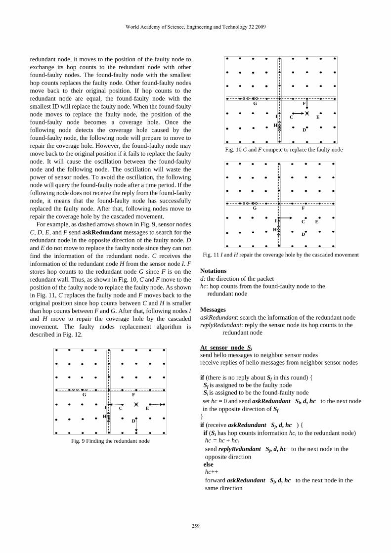
For example, as dashed arrows shown in Fig. 9, sensor nodes C, D, E, and F send askRedundant messages to search for the redundant node in the opposite direction of the faulty node. D and E do not move to replace the faulty node since they can not find the information of the redundant node. C receives the information of the redundant node H from the sensor node I. F stores hop counts to the redundant node G since F is on the redundant wall. Thus, as shown in Fig. 10, C and F move to the position of the faulty node to replace the faulty node. As shown in Fig. 11, C replaces the faulty node and F moves back to the original position since hop counts between C and H is smaller than hop counts between F and G. After that, following nodes I and H move to repair the coverage hole by the cascaded movement. The faulty nodes replacement algorithm is described in Fig. 12.
C
D
E
FG
H
I
Fig. 9 Finding the redundant node
C
D
E
FG
H
I
Fig. 10 C and F compete to replace the faulty node
C
D
E
FG
H
I
Fig. 11 I and H repair the coverage hole by the cascaded movement
Notations� d: the direction of the packet hc: hop counts from the found-faulty node to the
redundant node Messages� askRedundant: search the information of the redundant node replyRedundant: reply the sensor node its hop counts to the
redundant node At sensor node Si send hello messages to neighbor sensor nodes receive replies of hello messages from neighbor sensor nodes if (there is no reply about Sf in this round) { Sf is assigned to be the faulty node Si is assigned to be the found-faulty node set hc = 0 and send askRedundant� Si, d, hc� to the next node in the opposite direction of Sf
} if (receive askRedundant� Sj, d, hc� ) { if (Si has hop counts information hci to the redundant node)
hc = hc + hci send replyRedundant� Sj, d, hc� to the next node in the opposite direction
else hc++ forward askRedundant� Sj, d, hc� to the next node in the same direction

7
} if (receive replyRedundant� Sj, d, hc� ) { forward replyRedundant� Sj, d, hc� to the next node in the same direction
} if (receive replyRedundant� Si, d, hc� ) { if (the position of Sf is not replaced by other nodes) move R to replace the faulty node Sf following nodes move to repair the coverage hole by the
cascaded movement }
Fig. 12 The faulty nodes replacement algorithm
IV. SIMULATION
A. Simulation environment In the simulation, our algorithm is implemented using the
ns-2 simulator (version 2.27). Sensor nodes are deployed as the grid structure in a 200m×200m square region and redundant nodes are randomly scattered around the sensing field. The distance and the communication range of each sensor node are both 20m. The speed of the mobile sensor node is 2.5 m/s.
In order to know the effectiveness in different network sizes, we simulate our algorithm in three scenes. The first scene is that 25 sensor nodes are deployed as 5×5 grid and 5 redundant nodes are randomly scattered around the sensing field. The second scene consists of 49 sensor nodes (7×7 grid) and 7 redundant nodes. The third scene consists of 81 sensor nodes (9×9 grid) and 9 redundant nodes.
Since our algorithm can form different kinds of redundant walls according to the application, we form three kinds of redundant walls, which are cross, 3, and 5-redundant walls to evaluate the effectiveness of different kinds of redundant walls. Besides, we compare our algorithm with T. Le’s algorithm in [5]. We measure the performance of both algorithms by four metrics: (1) the time to find the redundant node, (2) the relocation time, (3) the message complexity, and (4) the moving distance to replace the faulty node.
B. Simulation results
0
0.1
0.2
0.3
0.4
0.5
0.6
(25,5) (49,7) (81,9)( Number of Sensor Nodes , Number of Redundant Nodes )
Tim
e to
find
the
redu
ndan
t nod
e (s
)
T. Le's algorithmcross-redundant walls3-redundant walls5-redundant walls
Fig. 13 Time to find the redundant node (s)
As shown in Fig. 13, no matter what kinds of redundant
walls are, our algorithm spends less time to find the redundant node than T. Le’s algorithm. This is because our algorithm arranges redundant nodes to form redundant walls, whereas T.
Le randomly scatters redundant nodes around the sensing field. Since redundant walls are constructed in the position where the average distance to each sensor node is the shortest, each sensor node can find the redundant node more quickly from nearby redundant walls. Besides, in Fig. 13, we can observe that T. Le’s algorithm spends more time to find the redundant node when the network size increases. The reason is that the distance from the redundant node to each sensor node becomes longer when the network size increases. Thus, their algorithm needs more time to find the redundant node.
5
15
25
35
45
(25,5) (49,7) (81,9)
( Number of Sensor Nodes , Number of Redundant Nodes )Re
loca
tion
Tim
e (s
)
T. Le's algorithmcross-redundant walls3-redundant walls5-redundant walls
Fig. 14 Relocation time (s)
As shown in Fig. 14, no matter what kinds of redundant
walls are, our algorithm outperforms T. Le’s algorithm in the relocation time. Besides, the relocation time of T. Le’s algorithm increases dramatically as the network size increases. The reason is that T. Le’s algorithm replaces the faulty node by the direct movement, whereas our algorithm replaces the faulty node by the cascaded movement. When the network size increases, the distance between the redundant node and the faulty node is longer. As for the direct movement, the redundant node has to move a long distance to replace the faulty node alone. As for the cascaded movement, all nodes along the path move at the same time. That is, the long distance is shared by all nodes along the path. Thus, the relocation time is significantly reduced in our algorithm. As cross, 3, and 5 redundant walls shown in Fig. 14, 5-redundant walls outperform 3-redundant walls and 3-redundant walls outperform cross-redundant walls. This is because the more redundant walls will distribute redundant nodes more and shorten the distance from the faulty node to the redundant node. Thus, 5-redundant walls perform the best in the relocation time.
Mes
sage
Com
plex
ity
0
100
200
300
400
(25,5) (49,7) (81,9)( Number of Sensor Nodes , Number of Redundant Nodes )
T. Le's algorithmcross, 3, 5-redundant walls

8
Fig. 15 Message complexity Since the message complexity of cross, 3, and 5-redundant
walls are almost the same, we use one line to represent them. The message complexity stands for the message to arrange redundant nodes and to replace the faulty node. As shown in Fig. 15, the message complexity of our algorithm is less than that of T. Le’s algorithm. The reason is that T. Le broadcasts messages to search for the redundant node, whereas our algorithm only sends messages to one of the four directions due to the existence of redundant walls.
0
100
200
300
400
500
1 3 5Number of Faulty Nodes
Mov
ing
Dist
ance
s (m
)
T. Le's algorithmcross-redundant walls3-redundant walls5-redundant walls
Fig. 16 Moving distances (m)
As the moving distance shown in Fig. 16, T. Le’s algorithm
is better as the number of faulty nodes increases. This is because their algorithm assumed that the faulty node could broadcast the help message and choose a redundant node to replace it. However, when the sensor node failed accidentally, the accidental faulty node could not broadcast the help message to redundant nodes. Thus, the accidental faulty node would leave a permanent coverage hole. The permanent coverage hole could not be repaired even the sensor network still had redundant nodes. In our algorithm, even if the sensor node fails accidentally, found-faulty nodes can coordinate with each other and find the proper redundant node to replace the faulty node. Thus, our algorithm can work well upon the accidental node failure. Though we take more distances to coordinate between found-faulty nodes, we can solve the accidental node failure problem which they can not.
V. CONCLUSION In this paper, we propose a fast sensor relocation algorithm
to arrange redundant nodes to form redundant walls without GPS. Redundant walls are constructed in the position where the average distance to each sensor node is the shortest. Thus, redundant walls can guide the sensor node to find the redundant node in the minimum time. When the sensor node fails, our algorithm replaces the faulty node by the cascaded movement. Simulation results show that our algorithm can find the proper redundant node in the minimum time and reduce the relocation time with low message complexity.
ACKNOWLEDGMENT This research was supported in part by the National Science
Council of the Republic of China under contract NSC 97-2221-E-031-001.
REFERENCES [1] I. F. Akyildiz, W. Su, Y. Sankarasubramaniam, and E. Cayirci, “A Survey
on Sensor Networks,” IEEE Communication. Magazine, pp. 102-114, August 2002.
[2] N. Ahmed, S. S. Kanhere and S. Jha, “The Holes Problem in Wireless Sensor Networks� A Survey,” ACM SIGMOBILE Mobile Computing and Communications Review, vol. 9, no. 2, pp. 4-18, April 2005.
[3] A. Ghosh and S. K. Das, “Coverage and connectivity issues in wireless sensor networks� A survey,” Pervasive and Mobile Computing, vol. 4, no. 3, pp. 303-304, 2008.
[4] G. Wang, G. Cao, T. Porta, and W. Zhang, “Sensor Relocation in Mobile Sensor Networks,” Proceedings of IEEE INFOCOM, March 2005.
[5] X. Li, N. Santoro, and I. Stojmenovic, “Mesh-Based Sensor Relocation for Coverage Maintenance in Mobile Sensor Networks,” Proceedings of the 4th Int. Conf. on Ubiquitous Intelligence and Computing (UIC) (LNCS 4611), pp. 696-708, 2007.
[6] T. Le, N. Ahmed, S. Jha, “Location-free Fault Repair in Hybrid Sensor Networks,” Proceedings of the first ACM Int. Conf. Integrated Internet Ad Hoc and Sensor Networks, vol. 138, no. 23, May 2006.
[7] B. Hofmann-Wellenhof, H. Lichtenegger, and J. Collins, Global Positioning System: Theory and Practice, Fourth Edition, Springer Verlag, 1997.
[8] J. Borenstein and Y. Koren, “Obstacle Avoidance with Ultrasonic Sensors,” IEEE Journal of Robotics and Automation, vol. 4, no. 2, pp. 213-218, 1988.
[9] Q. Li and D. Rus, “Global Clock Synchronization in Sensor Networks,” IEEE Transactions on Computers, vol. 5, no. 2, February 2006.
[10] B. Sundararaman, U. Buy, and AD. Kshemkalyni, “Clock Synchronization for Wireless Sensor Networks: A Survey,” Ad-Hoc Networks, vol. 3, no. 3, pp. 281-323, May 2005.
[11] D. Niculescu and B. Nath, “Ad Hoc Positioning System (APS) Using AoA,” Proceedings of IEEE INFOCOM, 2003.
[12] J. Ash and L. Potter, “Sensor network localization via received signal strength measurements with directional antennas,” Proceedings of the Forty-Second Annual Allerton Conference on Communication, Control, and Computing, pp. 1861–1870, September 2004.
[13] N. Patwari, A.O. Hero III, J. Ash, R.L. Moses, S. Kyperountas, and N.S. Correal, “Locating the Nodes,’’ IEEE Signal Processing Magazine, vol. 22, no. 4, pp. 54–69, July 2005.