A Fast and Stable Feature-Aware Motion Blur Filter - NVIDIAresearch.nvidia.com/.../Guertin2013MotionBlur-small.pdf · A Fast and Stable Feature-Aware Motion Blur Filter Jean-Philippe

A Fast and Stable Feature-Aware Motion Blur FilterJean-Philippe Guertin, Morgan McGuire, and Derek Nowrouzezahrai

Figure 1: We render temporally coherent motion blur without any motion artifacts, even on animation sequences with complexdepth and motion relationships that are challenging for previous post-process techniques. All results are computed in about 3msat 1280 ⇥ 720 on a GeForce GTX480, and our filter integrates seamlessly with post-process anti-aliasing and depth of field.

AbstractHigh-quality motion blur is an increasingly important and pervasive effect in interactive graphics that, even in thecontext of offline rendering, is often approximated using a post process. Recent motion blur post-process filters(e.g., [MHBO12,Sou13]) efficiently generate plausible results suitable for modern interactive rendering pipelines.However, these approaches may produce distracting artifacts, for instance, when different motions overlap in depthor when both large- and fine-scale features undergo motion. We address these artifacts with a more robust samplingand filtering scheme that incurs only small additional runtime cost. We render plausible, temporally-coherentmotion blur on several complex animation sequences, all in just 3ms at a resolution 1280 ⇥ 720. Moreover, ourfilter is designed to integrate seamlessly with post-process anti-aliasing and depth of field.

Categories and Subject Descriptors (according to ACM CCS): I.3.7 [Computer Graphics]: Three-DimensionalGraphics and Realism—Color, shading, shadowing, and texture

1. Introduction

Motion blur is an essential effect in realistic image synthesis,providing important motion cues and directing viewing at-tention, and is one of the few effects that distinguishes high-quality film production renderings from interactive graphics.We phenomenologically model the perceptual cues of mo-tion blurred image sequences to approximate this effect withhigh quality using a simple, high-performance post-process.

We are motivated by work in offline motion blur post-processing [Coo86, ETH⇤09, LAC⇤11], where many of theinitial experiments applied reconstruction filters to stochas-tic sampling routines. Unfortunately, these approaches aretoo heavyweight for modern game engines, however manyof their ideas remain useful. Conversely, adhoc approaches(e.g., applying a Gaussian blur to moving objects) have ex-isted in various forms for several years, however the ques-tion of how to approach motion blur post-processing usinga well-founded methodology has only recently gained atten-

tion in the interactive rendering community. This methodol-ogy had first found use (and success) in post-process anti-aliasing [Lot09] and depth of field [Eng06] approaches.We target temporally-coherent and plausible high-qualitymotion blur that rivals super-sampled results, but on asmall performance budget and a simple implementation. Assuch, we build upon recent post-process motion blur fil-ters [MHBO12, Sou13] and address several of their limita-tions in order to produce high-performance, stable, feature-preserving and plausible motion blurred image sequences.

Contributions. Previous works rely on conservative as-sumptions about local velocity distributions at each pixel inorder to apply plausible, yet efficient, blurs. Unfortunately,distracting artifacts arise when these assumptions are bro-ken; this occurs when objects nearby in image-space movewith different velocities, which is unavoidable even in sim-ple scenes, or when objects under (relative) motion have ge-ometric features of different scales. We eliminate these ar-

NVIDIA Technical Report NVR-2013-003, November 26, 2013c� 2013 NVIDIA Corporation, Guertin, and Nowrouzezahrai. All rights reserved.

Jean-Philippe Guertin, Morgan McGuire, and Derek Nowrouzezahrai / A Fast and Stable Feature-Aware Motion Blur Filter

tifacts and compute stable motion blur for both simple andcomplex animation configurations. Our contributions are:

• an improved, variance-driven directional samplingscheme that handles anisotropic velocity distributions,

• a sample-weighting scheme that preserves unblurred ob-ject details and captures fine- and large-scale blurring, and

• a more robust treatment of tile boundaries, and interactionwith post-process anti-aliasing and depth of field.

We operate on g-buffers, captured at a single time instance,with standard rasterization. Our results are stable under an-imation, robustly handle complex motion scenarios, and allin about 3ms per frame (Figure 1). Since ours is an imagepost-process filter, it can readily be used in an art-driven con-text to generate non-physical and exaggerated motion blureffects. We provide our full pseudocode in Appendix A.

2. Previous Work and Preliminairies

Given the extensive work on motion blur, we discuss recentwork most related to our approach and refer interested read-ers to a recent survey on the topic [NSG11].

Sampling Analysis and Reconstruction. Cook’s seminalwork on distribution effects [Coo86] was the first to ap-ply different (image) filters to reduce artifacts in the con-text of stochastic ray-tracing and micropolygon rasteriza-tion. More recent approaches filter noise while retaining im-portant visual details, operating in the multi-dimensional pri-mal [HJW⇤08], wavelet [ODR09] or data-driven [SD12] do-mains. Egan et al. [ETH⇤09] specifically analyze the ef-fects of sample placement and filtering, in the frequencydomain of object motion, and propose sheared reconstruc-tion filters that operate on stochastically distributed spatio-temporal samples. Lehtinen et al. [LAC⇤11] use sparse sam-ples in ray-space to reconstruct the anisotropy of the spatio-temporal light-field at a pixel and reconstruct a filtered pixelvalue for distribution effects. These latter two techniquesaim to minimize integration error given fixed sampling bud-gets in stochastic rendering engines. We also reduce visi-ble artifacts due to low-sampling rates, however we limitourselves to interactive graphics pipelines where distributedtemporal sampling is not an option and where compute bud-gets are on the order of milliseconds, not minutes.

Stochastic Rasterization. Recent work on extending tri-angle rasterization to support the temporal- and lens-domains [AMMH07], balances the advantages and dis-advantages of GPU rasterization, stochastic ray-tracing,and modern GPU micropolygon renderers [FLB⇤09]. Here,camera-visibility and shading are evaluated at many sam-ples in space-lens-time. Even with efficient implementationson conventional GPU pipelines [MESL10], these approachesremain too costly for modern interactive graphics applica-tions. Still, Shirley et al. [SAC⇤11] discuss image-space fil-ters for plausible motion blur given spatio-temporal output

from such stochastic multi-sample renderers. We are moti-vated by their phenomenological analysis of motion blur be-haviour and extend their analysis to more robustly handlecomplex motion scenarios (see Section 4).

Interactive Heuristics. Some approaches blur albedo tex-tures prior to texture mapping (static) geometry [Lov05] orextrude object geometry using shaders [TBI03], howeverneither approach properly handles silhouette blurring, result-ing in unrealistic motion blur. Max and Lerner [ML85], andPepper [Pep03], sort objects by depth, blur along their ve-locities, and compose the result in the final image, but thisstrategy fails when a scene invalidates the painter’s visibilityassumption. Per-pixel variants of this approach can reduceartifacts [Ros08,RMM10], especially when image velocitiesare dilated prior to sampling [Sou11, KS11], however thiscan corrupt background details and important motion fea-tures when multiple objects are present.

Motivated by recent tile-based, single blur velocity ap-proaches [Len10, MHBO12, ZG12, Sou13] (see Section 3),we also dilate velocities to reason about large-scale motionbehavior while sampling from the original velocity field toreason about the spatially-varying blur we apply. However,we additionally incorporate higher-order motion informationand feature-aware sample weighting to produce results thatare stable and robust to complex motion, effectively elim-inating the artifacts present in the aforementioned “single-velocity” approaches. Specifically, we robustly handle:

• interactions between many moving and static objects,• complex temporally-varying depth relationships,• correct blurring regardless of object size or tile-alignment,• feature-preservation for static objects/backgrounds.

We build atop existing state-of-the-art tile-based plausiblemotion blur approaches, detailed in Section 3, and presentour more robust multi-velocity extensions in Section 4.

3. Tile-Based Dominant Velocity Filtering Overview

We base our approach on recent single-velocity tech-niques [Len10, MHBO12, ZG12, Sou13] that combine phe-nomenological motion analysis and sampling-aware recon-struction filters. Figure 2 outlines the operation of these ap-proaches: first, the image is split into square r ⇥ r tiles ac-cording to a maximum blur radius r in image-space, ensur-ing that each pixel can at most be influenced by its (1-ring)neighboring tiles; secondly, a single dominant neighborhoodvelocity direction is determined at each tile; finally, the colorat the pixel is combined with weighted color samples alongthe dominant blur direction.

We review some notable details of this approach below:

• a tile’s dominant velocity vmax (Figure 2b; green) is com-puted in two steps: maximum per-pixel velocities are re-tained per-tile (Figure 2a,b; green, blue), and a 1-ringmaximum of the per-tile maxima yields vmax,


Pixel Velocities Max Tile Single VelocityVelocities Sampling

Figure 2: Motion blur with “single-velocity” techniques.

• pixels are sampled exclusively along vmax, yielding highcache coherence but ignoring complex motions, and

• each sample’s weight is computed using a depth-awaremetric that only considers the magnitude of velocities atthe source and sample points.

The "‘TileMax"’ pass can be computed in two passes, oneper image dimension, to greatly improve performance at thecost of a slight increase in memory usage. Samples are jit-tered to reduce (but not eliminate; see Section 4.5) banding,and samples are weighted (Figure 2c) to reproduce the fol-lowing phenomenological motion effects:

1. a distant pixel/object blurring over the shading pixel,2. transparency at the shading pixel from its motion, and3. the proper depth-aware combination of effects 1 and 2.

These techniques generate plausible motion blur with asimple, high-performance post-process and have thus al-ready been adopted in production game engines; however,the single dominant velocity assumption, coupled with thesample weighting scheme, results in noticeable visual arti-facts that limit their ability to properly handle: overlappingobjects that move in different directions, tile boundaries, andthin objects (see Figures 3, 6, 7, 11, 12 and 15).

We identify, explain, and evaluate new solutions for theselimitations. We follow the well-founded phenomenologicalmethodology established by single-velocity approaches andother prior work [Len10,SAC⇤11,MHBO12,ZG12,Sou13],and our technique maintains high cache coherence and paral-lelizable divergence-free computation for an equally simpleand high-performance implementation.

4. Stable and Robust Feature-Aware Motion Blur

We motivate our improvements by presenting artifacts inexisting (single-velocity) approaches. We demonstrate clearimprovements in visual quality with negligible additionalcost. Furthermore, our supplemental video illustrates the sta-bility of our solution under animation and on scenes withcomplex geometry, depth, velocity and texture.

4.1. Several Influential Motion Vectors.

The dominant velocity assumption breaks down when a tilecontains pixels with many different velocities, resulting in

Single Direction Ours

Figure 3: Top: an animation with complex depth and mo-tion relationships. The camera is moving upwards and thecar is doing a sharp turn while moving up. Bottom: single-velocity approaches (left) cannot handle these cases, result-ing in distracting artifacts both inside and between tiles; ourfilter (right) generates the correct plausible blur and is tem-porally stable (see video).

both an incorrect blur inside a tile and blur mismatches be-tween tiles (see Figures 3 and 6). This can occur, for exam-ple, with rotating objects (see Figure 7), objects with fea-tures smaller than a tile (see Figure 11), or when the viewand motion directions are (nearly) parallel (see Figure 6).

Specifically, by exploiting this assumption to reduce thesampling domain to 1D, single-velocity approaches weightsamples along vmax according only to the magnitudes oftheir velocities, and not the directions. This can result inoverblurred shading when samples (that lie along the dom-inant direction) should otherwise not contribute to the pixelbut are still factored into the sum, especially if they are mov-ing quickly (i.e., have large velocity magnitudes).

To reduce these artifacts we sample along a second, care-fully chosen direction. Moreover, we split samples betweenthese two directions according to the variance in the neigh-borhood’s velocities, while also weighting samples using alocally-adaptive metric based on the deviation of sample ve-locities from the blur direction. This scheme better resolvescomplex motion details and still retains cache coherence bysampling along (fixed) 1D domains. Section 5 details our al-gorithm and we provide pseudocode in Appendix A.

Local Velocity Sampling. If a pixel’s velocity differs sig-nificantly from the dominant direction, then it should also beconsidered during sampling. As such, we sample along boththe pixel’s velocity and the dominant velocity directions.This immediately improves the blur for scenes with com-plex pixel- and neighborhood-velocity relationships (e.g.,Figure 3), however at the cost of increased noise since we areeffectively halving the sampling rate in each 1D sub-domain.

If the pixel’s velocity is negligible, this scheme effectively“wastes” all the integration samples placed on the second di-rection. In these cases, we replace the pixel’s velocity with


the velocity perpendicular to the dominant direction, sam-pling along this new vector for half of the total samples andin the dominant direction for the other half. This helps in sce-narios where the dominant velocity entirely masks smallervelocities with different directions, in the neighborhood, andthe perpendicular direction serves as a "best-guess" to maxi-mize the probability of sampling along an otherwise ignoredimportant direction. Of course, if no such important (albeitsecondary) direction exists, then we are left with a similarsituation where samples placed along this perpendicular di-rection are “wasted”.

We ultimately combine the ideas of pixel (v(p)) andperpendicular-dominant (vmax(t)) velocities at the shadingpixel p’s tile t: we place a number (discussed below) of sam-ples along the center direction that interpolates between v(p)and v?max(t) as the pixel’s velocity diminishes past a mini-mum user threshold g (see Figure 4),

vc(p) = lerp⇣

v(p),v?max(t),(kv(p)k�0.5)/g⌘. (1)

Figure 4: Sampling di-rections vmax (green), v?max(yellow) and v(p) (blue).

Sampling along both vmax(t)and vc(p) ensures that eachsample contributes usefully tothe final blur, better capturingcomplex motion effects. Thisapproach remains robust whenthe pixel’s velocity is low (orzero, for static objects; see Fig-ures 3 and 6).

The number of sampleswe place along vc, and theirweights (both along vc andvmax), plays an important role in the behavior and quality ofthe motion blur. We address the problems of assigning sam-ples to each direction, and weighting them, separately. Wefirst discuss the distribution of samples over these two di-rections, and only later discuss a more accurate scheme forweighting their individual contributions. Our final samplingscheme is robust to complex scenes and stable under anima-tion.

Tile Variance for Sample Assignment. We first ad-dress the segmentation and assignment of samples tovc and vmax. In cases where the dominant velocity as-sumption holds, we should sample exclusively from vmax,

Figure 5: Variance(green) for tiles neigh-boring the pixel p (red).

as the standard single-velocityapproaches [Len10, MHBO12,ZG12, Sou13] do; however, it israre that this assumption holdscompletely and we would liketo find the ideal assignment ofsamples to the two directions inorder to simultaneously capturemore complex motions whilereducing noise. This amounts

to minimizing the number of“wasted” samples. To do so, wepropose a simple variance estimation metric.

At each tile, we first compute the angular variation be-tween a tile’s and its neighbor’s maximum velocities as

u(t) = 1� 1|N | Â

t2Nabs [vmax(t)] · abs

⇥vmax(t)

⇤, (2)

where N is the (1-ring) neighborhood tile set around (andincluding) t. The variance 0 u 1 is larger when neigh-boring tile velocities differ from vmax(t), and smaller whenthey do not. As such, we can use u(t) to determine the num-ber of samples assigned to vc and vmax with: u⇥N assignedto vc and (1�u)⇥N assigned to vmax (Figure 5).

This metric works well in practice, significantly reducingdistracting visual artifacts near complex motion while grace-fully reverting to distributing fewer samples along vc whenthe motion is simple; however, we require an extra (reduced-resolution) render pass (and texture) to compute (and store)u, which is less than ideal for pipeline integration (albeitwith negligible performance impact). We observe in prac-tice that, while the variance-based sample assignment doesimprove the quality of the result, conservatively splitting oursamples evenly between vc and vmax (i.e., N/2 samples foreach) generates roughly equal quality results (see Figure 6).

We note, however, that the weighting of each sample playsa sizeable role in both the quality of the final result and theability to properly and consistently reconstruct complex mo-tion blurs. We detail our new weighting scheme and contrastit to the scheme used in prior single-velocity approaches.

Single Direction Variance Velocity Direction

Figure 6: The lion in Sponza moving directly towards theviewer. Bottom: single-velocity results (left), our variance-based sample distribution (middle) conservative sample dis-tribution (right) both with vmax and vc direction sampling.


Single Direction Ours Without/With Blending

Figure 7: Tile edge artifacts. Bottom: single-velocity blur-ring (left) results in disturbing tile-edge artifacts that arereduced, in part, using multi-direction sampling (right; bot-tom) and, in full, with stochastic vmax blending (right; top).

Feature-Aware Sample Weights. Single-velocity ap-proaches compute weights by combining two metrics:

• depth difference between the sampled position and p, and• the magnitude of the velocity at the sample point and at p.

This does not consider that samples can still fall on objectsthat move in directions different than vmax (and even vc). Weinstead additionally consider the velocity direction at sam-ples when computing their weights. This yields a schemethat more appropriately adapts to fine-scale motions, withoutcomplicating the original scheme. Specifically, we will con-sider the dot product between blurring directions and sam-pled velocity directions. Recalling the three phenomenolog-ical motion blur effects in Section 3, we modify the weightscorresponding to each component as follows:

1. the contribution of distant objects blurring onto p, alongthe sampling direction, are (additionally) weighted by thedot product between the sample’s velocity direction andthe sampling direction (either vmax or vc, as discussed ear-lier); here, the total weight models the amount of colorthat blurs from the distant sample onto p and, as such, canbe modulated as the velocity at the sample vs differs fromthe blurring/sampling direction,

2. the transparency caused by p’s blur onto its surrounding is(additionally) weighted by the dot product of its velocity(actually, vc) and the dominant blur direction vmax; here,the total weight models the visibility of the backgroundbehind the pixel/object at p and, as such, if vc differs fromvmax, the contribution should reduce appropriately, and

3. the single-velocity approaches include a correction termto both model the combination of the two blurring effectsabove and also account for discontinuities along object

edges; we (additionally) multiply the weight for this termby the maximum of the two dot products above; here, themaximum is a conservative estimate that errs on the sideof slightly oversmoothing any such edges.

These simple changes (see pseudocode in Appendix A) sig-nificantly improve quality within and between tiles, particu-larly when many motion directions are present (Figure 6).

4.2. Tile Boundary Discontinuities.

Figure 8: Adapting per-sample weights accord-ing to the fine-scale ve-locity information.

The tile-based nature of single-velocity approaches, combinedwith their exclusive dependenceon the dominant velocity, caneasily lead to distracting tile-boundary discontinuities whenblur directions vary significantlybetween tiles (see Figure 7). Thisoccurs when vmax differs sig-nificantly between adjacent tilesand, since the original approachsamples exclusively along vmax,neighboring tiles can end up be-ing blurred in completely different directions. Our samplingand weighting approaches (Section 4.1) already help to re-duce this artifact, but we continue to sample from vmax (albeitnot exclusively, and with a different weighing scheme), andso we remain sensitive (to a lesser extent) to quick changesin vmax (see Figures 9 and 7).

Figure 9: We jitter the vmax(t)sample with higher probabil-ity closer to tile borders.

To further reduce thisartifact, we stochasticallyoffset our lookup into theNeighborMax maximumneighborhood velocitytexture for pixels near atile edge. This effectivelytrades banding for noisein the image, around tileboundaries, along edgesin the vmax buffer. Thus,the probability of samplingalong the vmax of a neigh-boring tile falls off as apixel’s distance to a tile border increases (Figure 9); we usea simple linear fall-off with a controllable (but fixed; seeSection 5) slope t.

It is important to note that, while intuitively logical, lin-early interpolating between neighborhood velocities alongtile edges produces incorrect results. Indeed, not only is theinterpolation itself not well-defined (for instance, interpolat-ing two antiparallel velocities requires special care), but evenmore importantly, two objects blurring on one another withdifferent motion directions is not equivalent to blurring alongthe average of their directions. Doing so causes distracting


artifacts where the blur seems to wave and often highlights,as opposed to mask, tile boundaries.

4.3. Preserving Thin Features.

Single-velocity filtering ignores the (jittered) mid-point sam-ple closest to the pixel and instead explicitly weighs the colorat p by the magnitude of the p’s velocity, without consider-ing relative depth or velocity information (as with the re-maining samples). This was designed to retain some of apixel’s original color regardless of the final blur, but it is notrobust to scenes with thin features or large local depth/veloc-ity variation. Underestimating this center weight causes thinobjects to disappear or “ghost” (see Figure 11). Furthermore,the weight is not normalized and so its effect reduces as Nincreases. These artifacts are distracting and unrealistic, andthe weight’s dependence on N makes it difficult to control.

We instead set this center weight as wp = kvk�1 ⇥ N/k,where k is a user-parameter to bias its importance. We usek = 40 in all of our results (see Section 5 for all param-eter settings). The second term in wp serves as a pseudo-energy conservation normalization, making wp robust tovarying sampling rates N (unlike previous single-velocity ap-proaches). Lastly, we do not omit the mid-point sample clos-est to p, treating it just as any other sample and applying ourmodified feature-aware sampling scheme (Section 4.1). Assuch, we also account for relative velocity variations at themidpoint, resulting in plausible motion blur robust to thinfeatures and to different sampling rates (see Figure 11).

4.4. Neighbor Blurring.

Both our approach and previous single-velocity approachesrely on an efficient approximation of the dominant neigh-borhood velocity vmax. We present a modification toMcGuire et al.’s [MHBO12] scheme that increases ro-bustness by reducing superfluous blur artifacts presentwhen the vmax estimate deviates from its true value.Specifically, the NeighborMax pass in [MHBO12] con-servatively computes the maximum velocity using theeight neighboring tiles (see Section 3 and Figure 2b),which can potentially result in an overestimation ofthe actual maximum velocity affecting the central tile.

Figure 10: Off-axisneighbors are only usedfor vmax computation ifthey will blur over thecentral tile.

We instead only consider a di-agonal tile in the vmax computa-tion if its maximum blur direc-tion would in fact affect the cur-rent tile. For instance, if the tile tothe top-left of the central tile hasa maximum velocity that does notpoint towards the middle, it isnot considered in the vmax com-putation (Figure 10). The reason-ing is that slight velocity devia-tions at on-axis tiles can result in

Single Ours Single Ours Single OursN = 17 N = 25 N = 45

Figure 11: Thin objects like the flagpole in Sponza ghost,to varying degrees depending on the sampling rate, with thesingle-velocity approach. Our approach resolves these de-tails and is robust to changes in the sampling rate.

blurs that overlap the middle tile,however larger deviations are re-quired at the corner (off-axis) tiles.

4.5. Stochastic Noise and Post-Process Anti-Aliasing

We have discussed how to choose the direction along whichto place each sample (either vmax or vc) as well as how toweight them (Section 4.1), however we have not discussedwhere to place samples along the 1D domain. Numericalintegration approaches are sensitive to sample distributionand, in the case of uniform samples distributed over our1D domain, the quality of both ours and the single-velocitytechniques can be significantly influenced by this choice.McGuire et al. [MHBO12] use equally-spaced uniform sam-ples and jitter the pattern at each pixel using a hashed noisetexture. This jittered uniform distribution has been recentlyanalyzed in the context of 1D shadowing problems with lin-ear lights [RAMN12] where it was proven to reduce variancebetter than low-discrepancy and stratified sampling.

We modify this strategy for motion blur integration anduse a deterministic Halton sequence [WLH97] to jitter theper-pixel sample sets with a larger maximum jitter value h(in pixel units), which improves the quality of the results;furthermore, as discussed earlier, we do not ignore the cen-tral sample closest to p and, as such, properly take its relativedepth and local-velocity into account during weighting.

Noise Patterns and Post-Process Anti-Aliasing. The noisepatterns produced by our stochastic integration are well-suited as input to post-processed screen-space anti-aliasingmethods, such as FXAA. Specifically, per-pixel jitter ensuresthat wherever there is residual noise, it appears as a high-frequency pattern that triggers the antialiasing luminanceedge detector (Figure 13, top right). The post-process an-tialiasing then blurs each of these pixels (Figure 13, bottomleft), yielding a result with quality comparable to roughlydouble the sampling rate (without FXAA; Figure 13, topleft). Stochastic vmax blending (Section 4.2) is compatiblewith this effect.

Furthermore, it is possible to maximize the noise smooth-ing properties of post-processed antialiasing by feeding a


Figure 12: Our motion blur results are temporally coherent and stable even in scenes with turbulent geometric deformation.

maximum-intensity, pixel-sized checkerboard to the edgedetector’s luminance input. This causes the antialiasing filterto detect edges on all motion blurred pixels, thus suppress-ing residual motion blur sampling noise (Figure 13, bottomright).

5. Implementation and Results

All our results are captured live at 1280 ⇥ 720 on an In-tel Core i5 at 3.3GHz with 16GB RAM and an NVIDIAGTX480 with 1.5GB vRAM. We recommend that read-ers digitally zoom-in on our (high-resolution) results tonote fine-scale details. Since our filter implementationdoes not have any divergent code paths our perfor-mance, at this resolution, was consistently 3.2ms ± 5%.We use the same parameter settings for all our scenes:{N,r,t,k,h,g} = {25,40,1,40,0.95,1.5}. All intermedi-ate textures, TileMax, NeighborMax [MHBO12] andTileVariance (Section 4.1), are stored in UINT8 formatand sampled using nearest neighbor interpolation, exceptfor TileVariance that required a bilinear interpolant toeliminate residual tile boundary artifacts.

We note the importance of properly quantizing and en-coding the per-pixel velocity when using integer buffers forstorage (as is typically done in e.g. game engines). Specif-ically, a limitation in the encoding used in McGuire et al.’simplementation, V[x,y]= v(px,y)/2r+0.5, is that the x and y

No AA FXAA edges

FXAA FXAA with checkerboard

Figure 13: Our noise is well-suited for standard post-process FXAA edge-detection, and we can further “hint”FXAA using a pixel-frequency luminance checkerboard.

velocity components are clamped separately to ±r, causinglarge velocities to only take on one of four possible values:(±r,±r). Instead, we propose a clamping scheme that makesoptimal use of an integer buffer’s precision, normalizing ac-cording to the range [�r,r] as

V[x,y]=v(px,y)

2r ⇥ max(min(|v(px,y)|⇥E,r),0.5)|v(px,y)|+e +0.5 ,

where e = 10�5 and the exposure time E is in seconds.

We modify the continuous depth comparison function(zCompare) used by McGuire et al. to better support depth-aware fore- and background blurring as follows: instead ofusing a hard-coded, scene-dependent depth-transition inter-val, we use the relative depth interval

zCompare[za,zb]= min⇣

max⇣

0,1� (za�zb)min(za,zb)

⌘,1⌘,

where za and zb are both depth values. This relative testhas important advantages: it works on values in a scene-independent manner, e.g. comparing objects at 10 and 20z-units will give similar results to objects at 1000 and 2000 z-units. This allows smooth blending between distant objects,compensating for their reduced on-screen velocity coverage,all while remaining robust to arbitrary scene scaling.

Motivated by Sousa’s [Sou13] endorsement of McGuireet al.’s single-velocity implementation, which has alreadybeen used in several game engines, all our comparisons wereconducted against an optimized version of the open sourceimplementation provided by McGuire et al., with both ourHalton jittering scheme and our velocity encoding. Whilethe variance-based u metric for distributing samples betweenvmax and vc yields slightly improved results over e.g. a 50/50sample distribution, we observe no perceptual benefit in us-ing u during interactive animation; as such, we disabled thisfeature in all our results (except Figure 6, middle zoom-in).

Post-Process Depth of Field. Earlier, we discussed our ap-proach’s integration with FXAA, a commonly used post-process in modern game engines. Another commonly usedpost-process effect is depth of field (DoF); however, thecombination of DoF and motion blur post-processes is a sub-ject of little investigation. We implemented the post-processDoF approach of Gilham in ShaderX5 [Eng06] and brieflydiscuss its interaction with our motion blur filter. Specifi-cally, the correct order in which to apply the two filters is not


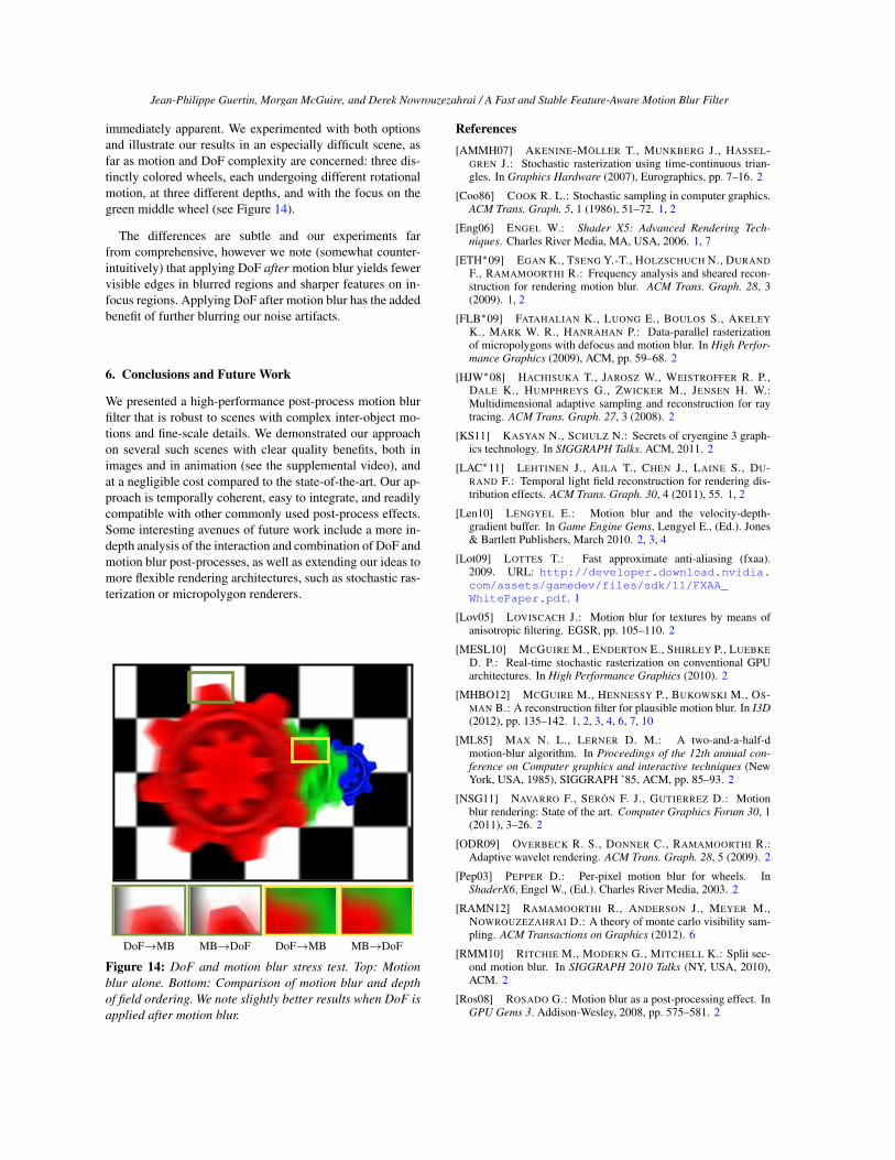
immediately apparent. We experimented with both optionsand illustrate our results in an especially difficult scene, asfar as motion and DoF complexity are concerned: three dis-tinctly colored wheels, each undergoing different rotationalmotion, at three different depths, and with the focus on thegreen middle wheel (see Figure 14).

The differences are subtle and our experiments farfrom comprehensive, however we note (somewhat counter-intuitively) that applying DoF after motion blur yields fewervisible edges in blurred regions and sharper features on in-focus regions. Applying DoF after motion blur has the addedbenefit of further blurring our noise artifacts.

6. Conclusions and Future Work

We presented a high-performance post-process motion blurfilter that is robust to scenes with complex inter-object mo-tions and fine-scale details. We demonstrated our approachon several such scenes with clear quality benefits, both inimages and in animation (see the supplemental video), andat a negligible cost compared to the state-of-the-art. Our ap-proach is temporally coherent, easy to integrate, and readilycompatible with other commonly used post-process effects.Some interesting avenues of future work include a more in-depth analysis of the interaction and combination of DoF andmotion blur post-processes, as well as extending our ideas tomore flexible rendering architectures, such as stochastic ras-terization or micropolygon renderers.

DoF!MB MB!DoF DoF!MB MB!DoF

Figure 14: DoF and motion blur stress test. Top: Motionblur alone. Bottom: Comparison of motion blur and depthof field ordering. We note slightly better results when DoF isapplied after motion blur.

References[AMMH07] AKENINE-MÖLLER T., MUNKBERG J., HASSEL-

GREN J.: Stochastic rasterization using time-continuous trian-gles. In Graphics Hardware (2007), Eurographics, pp. 7–16. 2

[Coo86] COOK R. L.: Stochastic sampling in computer graphics.ACM Trans. Graph. 5, 1 (1986), 51–72. 1, 2

[Eng06] ENGEL W.: Shader X5: Advanced Rendering Tech-niques. Charles River Media, MA, USA, 2006. 1, 7

[ETH⇤09] EGAN K., TSENG Y.-T., HOLZSCHUCH N., DURANDF., RAMAMOORTHI R.: Frequency analysis and sheared recon-struction for rendering motion blur. ACM Trans. Graph. 28, 3(2009). 1, 2

[FLB⇤09] FATAHALIAN K., LUONG E., BOULOS S., AKELEYK., MARK W. R., HANRAHAN P.: Data-parallel rasterizationof micropolygons with defocus and motion blur. In High Perfor-mance Graphics (2009), ACM, pp. 59–68. 2

[HJW⇤08] HACHISUKA T., JAROSZ W., WEISTROFFER R. P.,DALE K., HUMPHREYS G., ZWICKER M., JENSEN H. W.:Multidimensional adaptive sampling and reconstruction for raytracing. ACM Trans. Graph. 27, 3 (2008). 2

[KS11] KASYAN N., SCHULZ N.: Secrets of cryengine 3 graph-ics technology. In SIGGRAPH Talks. ACM, 2011. 2

[LAC⇤11] LEHTINEN J., AILA T., CHEN J., LAINE S., DU-RAND F.: Temporal light field reconstruction for rendering dis-tribution effects. ACM Trans. Graph. 30, 4 (2011), 55. 1, 2

[Len10] LENGYEL E.: Motion blur and the velocity-depth-gradient buffer. In Game Engine Gems, Lengyel E., (Ed.). Jones& Bartlett Publishers, March 2010. 2, 3, 4

[Lot09] LOTTES T.: Fast approximate anti-aliasing (fxaa).2009. URL: http://developer.download.nvidia.com/assets/gamedev/files/sdk/11/FXAA_WhitePaper.pdf. 1

[Lov05] LOVISCACH J.: Motion blur for textures by means ofanisotropic filtering. EGSR, pp. 105–110. 2

[MESL10] MCGUIRE M., ENDERTON E., SHIRLEY P., LUEBKED. P.: Real-time stochastic rasterization on conventional GPUarchitectures. In High Performance Graphics (2010). 2

[MHBO12] MCGUIRE M., HENNESSY P., BUKOWSKI M., OS-MAN B.: A reconstruction filter for plausible motion blur. In I3D(2012), pp. 135–142. 1, 2, 3, 4, 6, 7, 10

[ML85] MAX N. L., LERNER D. M.: A two-and-a-half-dmotion-blur algorithm. In Proceedings of the 12th annual con-ference on Computer graphics and interactive techniques (NewYork, USA, 1985), SIGGRAPH ’85, ACM, pp. 85–93. 2

[NSG11] NAVARRO F., SERÓN F. J., GUTIERREZ D.: Motionblur rendering: State of the art. Computer Graphics Forum 30, 1(2011), 3–26. 2

[ODR09] OVERBECK R. S., DONNER C., RAMAMOORTHI R.:Adaptive wavelet rendering. ACM Trans. Graph. 28, 5 (2009). 2

[Pep03] PEPPER D.: Per-pixel motion blur for wheels. InShaderX6, Engel W., (Ed.). Charles River Media, 2003. 2

[RAMN12] RAMAMOORTHI R., ANDERSON J., MEYER M.,NOWROUZEZAHRAI D.: A theory of monte carlo visibility sam-pling. ACM Transactions on Graphics (2012). 6

[RMM10] RITCHIE M., MODERN G., MITCHELL K.: Split sec-ond motion blur. In SIGGRAPH 2010 Talks (NY, USA, 2010),ACM. 2

[Ros08] ROSADO G.: Motion blur as a post-processing effect. InGPU Gems 3. Addison-Wesley, 2008, pp. 575–581. 2

http://developer.download.nvidia.com/assets/gamedev/files/sdk/11/FXAA_WhitePaper.pdf




Single Direction Ours Single Direction Ours Single Direction Ours

Single Direction Ours Single Direction Ours Single Direction Ours

Figure 15: Our results are temporally stable on complex scenes where previous approaches suffer from distracting artifacts.

[SAC⇤11] SHIRLEY P., AILA T., COHEN J. D., ENDERTON E.,LAINE S., LUEBKE D. P., MCGUIRE M.: A local image re-construction algorithm for stochastic rendering. In I3D (2011),pp. 9–14. 2, 3

[SD12] SEN P., DARABI S.: On filtering the noise from the ran-dom parameters in monte carlo rendering. ACM Trans. Graph.31, 3 (2012), 18. 2

[Sou11] SOUSA T.: Cryengine 3 rendering techniques. In Mi-crosoft Game Technology Conference. August 2011. 2

[Sou13] SOUSA T.: Graphics gems from cryengine 3. In ACMSIGGRAPH Course Notes (2013). 1, 2, 3, 4, 7

[TBI03] TATARCHUK N., BRENNAN C., ISIDORO J. R.: Motionblur using geometry and shading distortion. In ShaderX2: ShaderProgramming Tips and Tricks with DirectX 9.0, Engel W., (Ed.).2003. 2

[WLH97] WONG T.-T., LUK W.-S., HENG P.-A.: Samplingwith hammersley and halton points. J. Graph. Tools 2, 2 (1997),9–24. 6

[ZG12] ZIOMA R., GREEN S.: Mastering DirectX 11with Unity, March 2012. Presentation at GDC 2012https://developer.nvidia.com/sites/default/files/akamai/gamedev/files/gdc12/GDC2012_Mastering_DirectX11_with_Unity.pdf. 2, 3, 4

https://developer.nvidia.com/sites/default/files/akamai/gamedev/files/gdc12/GDC2012_Mastering_DirectX11_with_Unity.pdf




Acknowledgements

The NeighborMax tile culling algorithm was contributed byDan Evangelakos at Williams College. Observations aboutFXAA, the use of the luminance checkerboard, and con-sidering the central velocity in the gather kernel are fromour colleagues at Vicarious Visions: Padraic Hennessy, BrianOsman, Michael Bukowski.

Appendix A: Pseudocode

We include pseudocode that depends on the following helperfunctions and shorthand operators: sOffset jitters a tilelookup (but never into a diagonal tile), rnmix is a vector lin-ear interpolation followed by normalization, norm returns anormalized vector, b·c returns the whole component, and &denotes bitwise and. Unless otherwise specified, we use thenotation/functions of McGuire et al. [MHBO12]. Our func-tion returns four values: the filtered color and luminancevalue to pass to an optional FXAA post-process.

function filter(p):let j = halton(�1,1)let vmax= NeighborMax[p/r+sOffset(p, j)]if (kvmaxk 0.5)return (color[X],luma(color[X]))

let wn = norm(vmax), vc = V[p],,! wp = (�wny,wnx)

if (wp ·vc < 0) wp =�wplet wc = rnmix(wp,norm(vc), (kvck�0.5)/g)

// Begin integration with the current point// (center weight) plet totalWeight= N/(k⇥kvck)let result= color[p]⇥totalWeight

for i 2 [0,N)let t= mix(�1,1,(i+ j⇥h+1)/(N +1)) // jitter

our sample

// Compute the sample point S; split samplesbetween {vmax,vc}

let d= vc if i odd or vmax if i evenlet T= t⇥kvmaxklet S= bt⇥dc+p

// Compute S’s velocity and colorlet vs = V[S], colorSample= color[S]

// Fore- vs. background classification of Y// relative to plet f = zCompare(Z[p],Z[S])let b = zCompare(Z[S],Z[p])

// This sample’s weight and velocity-aware factors// (Section 4.1)let weight= 0, wA= wc ·d, wB= norm(vs) ·d

// The three phenomenological cases// (Sections 3 and 4.1):// Objects moving over p, blur from p’s motion,// and their blendingweight += f ·cone(T,1/kvsk)⇥wBweight += b ·cone(T,1/kvck)⇥wAweight += cylinder(T,min(kvsk,kvck))

,! ⇥max(wA,wB)⇥2

totalWeight += weight // For normalizationresult += colorSample⇥weight

return (result/totalWeight,(px +py)&1)

Documents

A Fast and Stable Feature-Aware Motion Blur Filter - NVIDIAresearch.nvidia.com/.../Guertin2013MotionBlur-small.pdf · A Fast and Stable Feature-Aware Motion Blur Filter Jean-Philippe