A dynamic modeling approach to simulating socioeconomic ...csr.ufmg.br/modelagem_sistemas_dinamicos/wang_urban_dynamics.pdf · Ecological Modelling 140 (2001) 141–162 A dynamic

Ecological Modelling 140 (2001) 141–162

A dynamic modeling approach to simulating socioeconomiceffects on landscape changes

Yeqiao Wang *, Xinsheng ZhangDepartment of Natural Resources Science, Uni�ersity of Rhode Island, Kingston, RI 02881, USA

Abstract

Modeling and simulating the effects of human factors on landscape change remain as challenges for ecologicalstudies. In this paper, we present a dynamic landscape simulation (DLS) approach to elucidate human-inducedlandscape changes for a 5104 km2 study area within the Chicago metropolitan region. The DLS consists of an urbangrowth simulation submodel and a land-cover simulation submodel. This approach simulates urban land-useexpansion by incorporating socioeconomic and demographic data and predicts changes in the landscape as a resultof urban expansion. A utility function of spatial choice and a methodology for the construction of that utilityfunction were developed to execute the process. The approach, with dynamic adjustment of transition structures (i.e.the transition potentials, threshold and rate), overcomes the shortcomings of static and statistical models that use aconstant transition probability in simulation modeling. It also allows selected economic principles to be integratedinto landscape simulation. In this study, historical land-cover and census data were applied to derive transitionthresholds and transition rates of the land cover changes. Comparison of the 1997 land-cover maps derived by a DLSsimulation and by the classification of Landsat Thematic Mapper (TM) remotely sensed data indicated that a 62.3%overall agreement was achieved among the changed areas. Landscape simulations of the study area from 1997 to 2020at 5 year time interval were prepared. The results depicted the trends of landscape change in this large urban settingarea. © 2001 Elsevier Science B.V. All rights reserved.

Keywords: Dynamic model; Utility function; Urban growth; Landscape; Simulation; Chicago region

www.elsevier.com/locate/ecolmodel

1. Introduction

Landscape pattern has four basic elements:number, size, shape, and juxtaposition of patches.These elements are important contributors to theinterpretation of ecological processes (Gardner etal., 1987; O’Neill et al., 1988; Dunn et al., 1990).

Landscapes represent complex ecological systemsthat operate over broad spatio-temporal scales(O’Neill et al., 1989). Considerable interest hasfocused on the simulation of landscape dynamics(e.g. Turner, 1987; Turner, et al., 1989; Mullerand Middleton, 1994; Boerner et al., 1996;Childress, 1997). Since a landscape pattern at anygiven time is a stage on which dynamic processesoccur, quantitative landscape studies require thattime, or temporal change, be considered (Dunn etal., 1990).

* Corresponding author. Tel.: +1-401-8744345; fax: +1-401-8744561.

E-mail address: [email protected] (Y. Wang).

0304-3800/01/$ - see front matter © 2001 Elsevier Science B.V. All rights reserved.

PII: S0304 -3800 (01 )00262 -9

Y. Wang, X. Zhang / Ecological Modelling 140 (2001) 141–162142

Both natural and socioeconomic processes drivelandscape change. Among human factors, urbanland expansion is one of the main driving forcesthat changes landscapes and threatens naturalecosystems. Human demand for land and exten-sive land conversion for economic activities accel-erate losses of biodiversity (Ehrlich, 1988; Liu andAshton, 1998). Socioeconomic and demographicdata have, until recently, rarely been linked withother biophysical data in landscape studies (Loand Faber, 1997). Simulation of human-influ-enced landscape change remains as a researchchallenge (Flamm and Turner, 1994).

Modeling approaches that incorporate humanfactors into landscape simulation have long beenexplored (Turner, 1987; Hall et al., 1988). Flammand Turner (1994) tested stochastic simulationmodels to integrate socioeconomic and ecologicalinformation into a spatially explicit transitionmodel of landscape change. Their simulationswere designed to compare pixel-based (100 m),patch-based, and ownership-based transitionmodels in order to evaluate the effects of incorpo-rating differing amounts of information about thelandscape into the model. Socioeconomic datawere applied to construct transition probabilitiesand introduce human influences into landscapesimulations.

When human activities are considered, Markovmodels which handle stationary processes maynot be appropriate, because transition probabili-ties among landscape states are not constant(Boerner et al., 1996). Traditional cellular au-tomaton (CA) models do not consider variationof transition structures throughout a large studyarea in which unbalanced human influences onlandscapes may occur. A hybrid Markov-cellularautomaton (M-CA) model is a new approach inspatio-temporal dynamic modeling (Silvertown etal., 1992; Li and Reynolds, 1997). In M-CA mod-eling, the Markov process controls temporal dy-namics among the cover types through the use oftransition probabilities (e.g. Turner, 1987; Silver-town et al., 1992). Spatial dynamics are controlledby local rules determined either by the cellularautomaton mechanism (neighborhood configura-tion) or by its association with the transitionprobability (e.g. Silvertown et al., 1992). It has

been recognized that GIS data have great poten-tial for M-CA modeling, both in the model devel-opment and simulation phases (Zhou andLiebhold, 1995). A major advantage of the M-CAapproach is that GIS and remote sensing data canbe efficiently incorporated (Li and Reynolds,1997). In particular, temporal GIS data can beused to define initial conditions, to parameterizeM-CA models, to calculate transition probabili-ties and to determine the neighborhood rules.Although the potential has been discussed by Liand Reynolds (1997), multitemporal remote sens-ing data and the derivatives of sequentially devel-oped GIS data have rarely been directlyincorporated into dynamic simulation modeling.

Since urban land expansion is one of the mainfactors that affects natural ecosystems, a dynamicmechanism in urban growth simulation is a keyfor revealing human impacts on landscapechange. GIS spatial analysis provides support forformulating operational and practical urban andregional models. In general, four categories ofGIS-based models have been applied to predictthe evolution of urban and regional spatial struc-tures. These include statistical models (Jensen etal., 1994); Lowry-type models (Parrot and Stutz,1991); spatial choice behavior models (Zhang andHe, 1997); and CA models (Xie, 1996; Clarke andGaydos, 1998; Wu, 1998). Spatio-temporal inter-actions among the spatial compartments and sub-systems were not considered as an integralcomponent of the models. Most of these modelscannot describe dynamic structures of urban sys-tems when spatial interactions among system ele-ments are required and when the dynamicevolution of urban spatial structure needs to beconsidered.

In order to reveal human-induced landscapechange, we developed a dynamic landscape simu-lation (DLS) approach. The DLS incorporatesand quantifies socioeconomic and demographicfactors using utility functions of spatial choice.This new approach differs from the previous staticand statistical models in that it enables economicprinciples, such as utility and marginal utility, tobe imbedded directly in landscape simulation. Dy-namic adjustments of transition rates andthresholds were implemented in the DLS coupled

Y. Wang, X. Zhang / Ecological Modelling 140 (2001) 141–162 143

by the use of multiscale spatial units. The DLScreates a new mechanism to study the impact ofhuman factors on landscape dynamics. Therefore,the objective of this paper is to illustrate the DLSmodeling approach and the testing results. We firstintroduce the model structure. Then, we discuss themethods for model construction. Finally, as anapplication example, we simulate the landscapechange within the metropolitan Chicago area usingthe DLS approach.

2. Methods

2.1. Study area

The study area is located in a semicircular zonebetween 30 and 65 km from the center of downtownChicago and is about 5104 km2 in area. TheChicago metropolitan area contains some of theworld’s best remaining patches of endangered nat-ural communities. This significant concentration ofrare natural ecosystems includes eastern tallgrassprairie, oak-savanna, open woodland, and woodedand prairie wetland. The existing patches are smalland isolated. Long-term survival of these commu-nities depends on proper management of muchlarger, restorable acreage that surrounds and con-nects the high-quality remnants. Like mostmetropolitan areas, the Chicago region has experi-enced dramatic land-cover change in the past threedecades. Population increase and employment-re-lated decentralization of population are among thedominant driving factors that result in landscapechange. For example, from 1970 to 1990, theregion’s population and employment increased by4 and 21%, respectively, while the urban land areaincreased by 47%. Land-cover changes occurredmostly in the suburban areas where there areconcentrations of natural preserves. As recentlyprojected by the U.S. Bureau of the Census andendorsed by the Northeastern Illinois PlanningCommission (NIPC), the Chicago region’s popula-tion and employment will grow by the year 2020to more than 9 million and to 5.3 million, a 25 and37% increase from 1990, respectively (NIPC, 1998).The impacts of the projected population and em-ployment increases on the region’s landscape are

unknown. Urban land expansion accelerates frag-mentation and degradation of natural communitiesin this large urban setting environment. What theeffects of socioeconomic and demographic changeson the landscape will be remains a question toanswer.

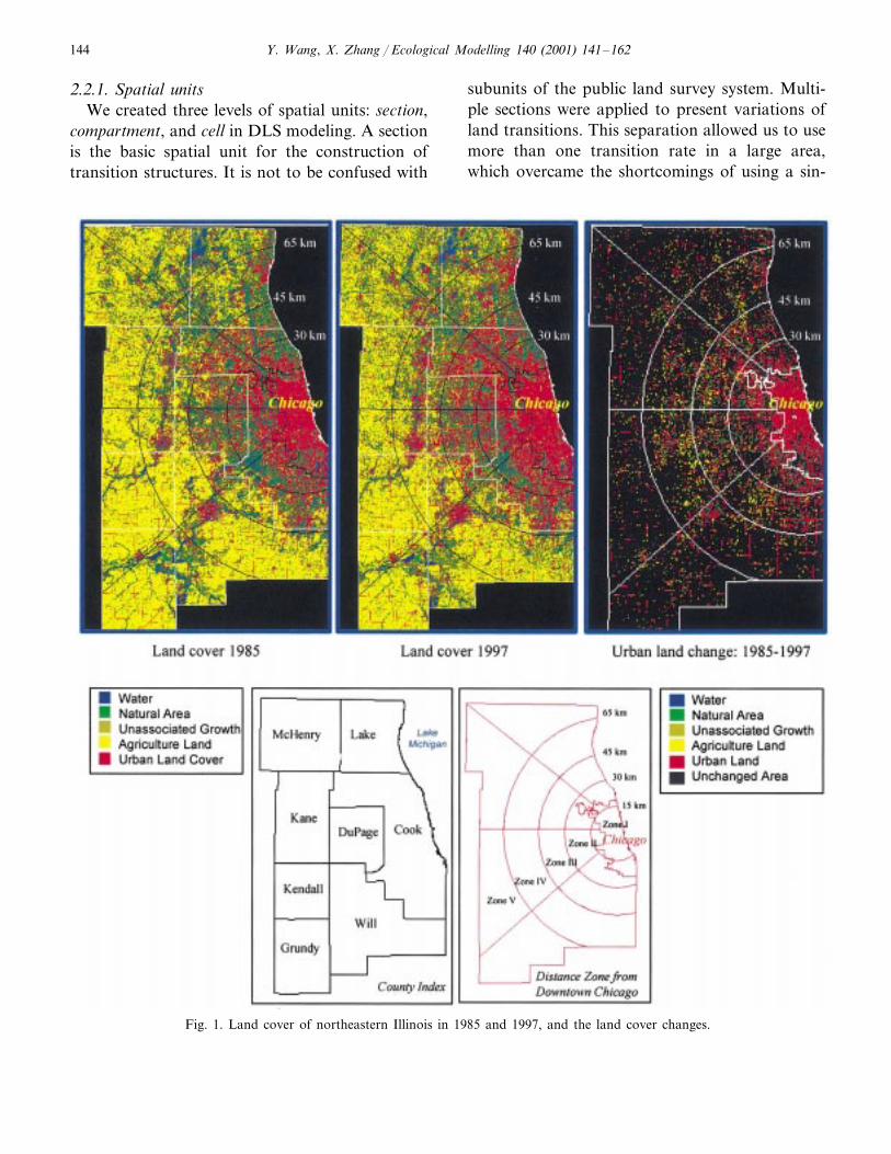
Distance from downtown Chicago is consideredan important character of the regional landscape.A half-ring pattern can be observed from bothLandsat images and the derivatives of land covermaps. We subjectively created five concentric zonesto quantify the half-ring pattern of the landscape(Fig. 1). The zones divided the Chicago metropoli-tan region into 0–15 km (Zone I), 15–30 km (ZoneII), 30–45 km (Zone III), 45–65 km (Zone IV), and�65 km (Zone V) areas. The distance was mea-sured from the center of Chicago. Land-coverinformation derived from 1997 Landsat ThematicMapper (TM) data revealed that Zone III and ZoneIV are among the most fragmented areas in theregion (Table 1). The highest patch densities ofnatural areas were observed in Zone III (4.05patches/km2) and in Zone IV (3.90 patches/km2).These two zones were the most changed areasbetween 1985 and 1997 in urban land expansion(Table 2). Population and employment forecastingdata (NIPC, 1998) indicate that the municipalitieswithin or close to these two zones will be amongthe most changed areas from year 1990–2020.Landscapes within these areas will be affecteddramatically by expanding urbanization. Thereforethese two zones were selected as the study area.

2.2. Model structure

The DLS consists of an urban growth simulationsubmodel and a land-cover simulation submodel(Fig. 2). The urban growth submodel simulates theurban land expansion driven by socioeconomic anddemographic factors. The land-cover simulationsubmodel predicts landscape change as the result ofurban spatial growth. The simulation is controlledby the spatial choice utility function. Socioeco-nomic and demographic data, land-cover data ofmultiple years derived from Landsat remotelysensed images, and multisource GIS data wereemployed to define the simulation conditions andrestrictions.


2.2.1. Spatial unitsWe created three levels of spatial units: section,

compartment, and cell in DLS modeling. A sectionis the basic spatial unit for the construction oftransition structures. It is not to be confused with

subunits of the public land survey system. Multi-ple sections were applied to present variations ofland transitions. This separation allowed us to usemore than one transition rate in a large area,which overcame the shortcomings of using a sin-

Fig. 1. Land cover of northeastern Illinois in 1985 and 1997, and the land cover changes.


Table 1Landscape patch density of the Chicago region in 1997

Distance and area of the Natural area Urban landUnassociated growth Agriculture land(Patches/km2) (Patches/km2) (Patches/km2)zones (Patches/km2)

0.93 1.12 0.33Zone I (0–15 km, 473.92 1.9km2)

2.65 2.94Zone II (15–30 km, 1187.65 0.62 3.38km2)

4.05Zone III (30–45 km, 2.9 1.41 3.361768.19 km2)

3.9 2.5 2.26Zone IV (45–65 km, 2.813335.43 km2)

Zone V (�65 km, 4887.67 3.39 2.32 2.58 2.19km2)

Fig. 2. The DLS model takes multi-year socioeconomic and demographic data, biophysical data, and multi-year land-cover data asinput. Urban growth simulation submodel and land-cover simulation submodel are integrated using utility function of spatial choice.Spatiotemporal interaction between two submodels is achieved by three levels of spatial units, i.e. section, compartment, and cell.The simulation is controlled by dynamic transition thresholds and rates, spatial constraints, and socioeconomic/demographic drivingfactors. The model output represents a dynamic series of landscape simulations.

gle transition rate to simulate the landscape of theentire region. Spatial location and landscape char-

acters of the region were referenced to design theeight sections for the study area (Fig. 3).

Y.

Wang,

X.

Zhang

/E

cologicalM

odelling140

(2001)141

–162

146

Table 2Urban land-cover changes of the study area, between 1985 and 1997, by zones

Unasso. growth to urban Urban land in Urban land change (%) Urban change densityLand cover Nature to urban Agriculture to urban(ha.) (ha./km2)change 1985 (ha.)(ha.) (ha.) 1985–1997

1.6338 059149 2.03295329Zone I48 037 16.92 6.84Zone II 32323559 1335

11.547428 62.01Zone III 32 9175505 747976.115049 7.267663 10 044 29 898Zone IV

23 992 52.81 4.04Zone V 48961739 6035


Compartments, 2.5×2.5 km areas within sec-tions, are the second level spatial unit. They con-trol the spatial step of the simulation for theurban growth submodel. Each compartment pos-sesses a set of state variables. The state variablesare constant at a given model iteration. Urbanizedarea in each compartment is calculated at a giventime interval �t based on the initial state condi-tion at time t. The change of urbanized land, as anew state variable of the compartment, representsa driving factor in landscape change. The size ofthe compartment was determined by referencingthe mean size of the polygons that represent the270 municipalities of the Chicago metropolitanregion.

The cell, sized at 150×150 m (5×5 LandsatTM pixels), is the minimum spatial unit in theDLS model. A cell reflects the land-cover status ata given time in this spatial unit. Under the controlof the expected urbanized area within each com-partment at time t+�t, the states of cells att+�t are simulated. Cells within different com-

partments have different controls for their ex-pected urban land areas. Changes of a cell’sland-cover types alter the state variable of thecompartment.

2.2.2. Urban growth simulation submodelThe urban growth simulation submodel is a key

to bridging the human driving factors and land-scape change. Only when urban growth can beeffectively modeled can the impacts of populationand employment increase on landscapes be accu-rately simulated. Therefore, an urban growth sim-ulation was designed as a submodel in this DLSapproach. The concepts of effective population,utility and marginal utilities, construction of util-ity function, and using these concepts in urbangrowth simulation are discussed as follows.

2.2.2.1. Effecti�e population. In this study, urbanland consumption is considered as residential-,commercial- and industrial-related land uses. Ef-

Fig. 3. Study area and the spatial units. Section is the basic spatial unit that is applied to construct transition structures;Compartment is the basic spatial unit for urban growth submodel. Compartment is 2.5×2.5 km in size. Cell is the minimum spatialunit for land-cover simulation submodel. Cell is 150×150 m in size and contains 5×5 Landsat TM pixels.


fective population (Peff is defined as the sum ofresidential population (Presi) and weighted numberof employment (Pempl) in a given spatial area.Square kilometer is applied as the given spatialarea.

Peff=Presi+R Pempl. (1)

Presi and Pempl are the hosts that consume residen-tial as well as commercial and industrial landuses. Peff reflects human effects on consumptionof land by the above land uses. Presi and Pempl canbe obtained from census and employment data. Inorder to calculate effective population, the R (Eq.(1)) is used to transform the number of employ-ment to the weighted number of employment. R isthe ratio between average urbanized areas occu-pied by residential and by employment in eachsection.

2.2.2.2. Spatial choice and the utility function. The-oretical studies of applying spatial choice utilityfunctions have been documented (Timmermanand Borgers, 1989; Leonardi and Papageorgiou,1992). In this study, spatial choice is a process inwhich effective population compares the at-tributes of the compartments within a feasible setof choices and chooses the most probable com-partment to occupy. Urban growth represents anexpansion of urban land-use that associates withspatial choice of effective population. We defineutility as a measure that the effective populationderives from the attributes within the selectedcompartments. A utility function, therefore, rep-resents a relationship between the quantities ofthe attributes of compartments that the effectivepopulation occupies and the utilities derived fromthe attributes. Each compartment has a utilityvalue. The utility functions are employed to deriveprobabilities of the compartments that are to beoccupied by effective population.

A section of the study area is divided into a setof compartments. Spatial location of a compart-ment is described by its central coordinates ofz={(x1, y1), (x2, y2), … (xz, yz}, where Z is thetotal number of compartments. The attribute vec-tor of z is specified as S(z ; t)={s1(z ; t), s2(z ; t),s3(z ; t) … sn(z ; t)}, where n is the number ofdimensions of attribute vectors that describes the

features of the compartments. The compartmentsdefine a discrete space for the utility function ofspatial choice. Spatial choice of the ith socioeco-nomic element is described by utility function as:

Ui(z ; t)= f [S(z ; t), Hi(t)]+�(t) i=1, 2, 3 … m)

(z ; t)� (Z ; t) z={(x1, y1), (x2, y2), … ,(xz yz)}(2)

where:

is the utility function associatedUi(z ; t):with spatial choices of location z(z=1, 2, 3, … Z) by the ith socioe-conomic element at time t ;

S(z ; t): is the attribute vector of compart-ment z at time t ;is the characteristic of the ith so-Hi(t):cioeconomic element at time t ;is the random disturbance at time�(t)t ;is the set of locations that have(Z; t):the potentials to be selected by theith socioeconomic element at timet ;is a geometric central coordinateZ= (x ; y):of the spatial compartment z ;is the total number of socioeco-m :nomic elements considered.

In the model, spatial choice depends on twofactors: landscape pattern (S(z ; t)) and character-istics of socioeconomic elements (Hi(t)). Humanactivities as one component of spatial choice canbe represented by a utility function.

2.2.2.3. Construction of the utility function. Toconstruct a utility function, we assume that thespatial distribution of effective population obeys autility function of spatial choice. If P(z) is thechange rate of the density of effective population,U is the utility function associated with spatialchoice of location by effective population, then

Pz=C U(k1, k2, … , kn), (3)

where C is a constant and can be defined as theratio of the change rate of effective population


and the utility value. It can be derived during theconstruction of utility functions. The kis representthe ith attributes that impact spatial choices ofeffective population. The attributes considered in-clude: (1) density of effective population; (2) em-ployment in a given compartment; (3) roaddensity; (4) degree of facility accessibility (Flammand Turner, 1994); (5) degree of transportationaccessibility which is the time-distance to majortransportation; and (6) proportion of non-urbanland in each compartment. All six attributes werenormalized to a range of 0–100.

To implement the above discussion, a utilityfunction needs to be constructed for each of theabove attributes kj (1� j�n, n=6) by finding aset of compartments which possess constant at-tributes for all ki (i� j ). Then kj is the onlyattribute that alters the changing rate of the den-sity of effective population.

In order to construct a utility function, a mar-ginal utility needs to be defined. A marginal utilityis the increment of utility caused by the unitincrease of certain attribute (Peterson, 1989). Themarginal utility Mu(kjl) is defined as:

Mu(kjl)=1C

�Pl

�kjl

(l=1, 2, … L), (4)

where L is the number of compartments in theselected set. �kjl is the increment of the influencefactor. �Pl is the increment of changing rate ofthe density of effective population caused by thechanges of the influence factor. A curve-fittingprocess can be applied to explore the relationsbetween influence factor kj and the change rate ofthe density of effective population. Let Mu(kj) bethe fitting curve function, the utility of kj is:

U(kj)=� kj

0

Mu(kj)dkj. (5)

Since the Kj has been normalized to a continu-ous variable between 0 and 100, the influencingimpact of Kj can be quantified. Following thesame process, utility functions for other influencefactors, U(k1), U(k2) … U(kn), can be derived. Bythe additive rule of utility (Mansfield, 1982), thetotal utility function of spatial choice for effectivepopulation is derived as:

U [k1(x, y), k2(x, y), … kn(x, y)]= �n

i=1

U [ki(x, y)].

(6)

The following example explains the methodol-ogy for constructing a utility function for theattribute U(k6) the proportion of non-urban land.The utility function in this example was derivedfor section 6 (Fig. 3). Applied data included:employment and residential data in 1985 and1996, land cover data in 1985 and 1997, and roaddensity. The influence factors of kj ( j=1, 2, …, 6)and the P(z) between 1985 and 1997 for the 255compartments within this section were derivedfrom the above data. Seventy-six compartmentsthat had the same influence factors of k1 throughk5 but different k6 were selected. Therefore L=76. The change rate of �P(z)/�k61 (l=1, 2, … , 76) was calculated. For each k61, acorresponding �P(z)/�k61 was observed. The re-lationship between k61 and �P(z)/�k61, which rep-resented the marginal utility value of k61, wascomputed (Fig. 4a). According to the law ofdiminishing marginal utility (Sher and Pinola,1981; Mansfield, 1982; Peterson, 1989), the addi-tional utility derived from the consumption of anadditional quantity of an attribute in the com-partments should decrease. Therefore, the fittingcurve of this relationship was expressed as anexponential relationship:

Mu(k6)=A exp (B k6), (7)

where A and B are constants which can be deter-mined by the 76 pairs of k61 and �P(z)/�k61. Themarginal utility function was derived (Fig. 4b).From the marginal utility function the con-structed utility function for the influence factor k6

in the selected section was obtained (Fig. 4c).

2.2.2.4. Simulating urban growth. A compartmentand a given iteration of the model are the basicspatio-temporal units for the simulation of urbangrowth. In this study, time interval �t was appliedas the time break in which the state of variableswould be adjusted. Every 5 years starting from1997 was defined as a time interval. An initialstate of the attributes for each of the compart-ments was obtained from multiple GIS data andcensus data. In each iteration, the attributes and


Fig. 4. The process for constructing a utility function. (a).Relationships between proportions of non-urban land at-tribute (k6) and the (�P/�k6); (b) marginal utility function; (c)utility function.

section in a given time interval �t. �P (t+ �t) isthe increment of effective population within theSth section in a given time interval �t. US (i, t) isthe utility of the ith compartment within the Sthsection at time t. Am

S is an average urban area foreach unit of effective population. Aa

s (i, t) is theavailable land within the ith compartment of theSth section at time t for urban expansion. Theavailable land was extracted from land cover databy excluding the areas of restrictions. The areas ofrestrictions include nature preserves, flood zones,buffered areas around urban constructions andmajor road networks, and other areas that arevery unlikely to be consumed by urbanization,such as water surface and wetland sites. Theconstant C in the utility function was obtainedwhen the allocated population (Eq. (8)) best ap-proximated to the distribution of census popula-tion. A search algorithm that applied the rule ofminimum of quadratic sum of residual was devel-oped to obtain the C. If there is no available landin one compartment, the unallocated effectivepopulation will be reallocated to the neighboringcompartments (Eq. (9)). In each model iteration,at first, the increment of effective population�PS (i, t+�t) is allocated (Eq. (8)). If Am

S �PS

(i, t+�t)�AaS (i, t), the allocation process stops.

Otherwise, unallocated effective �Pri in the ith

compartment is calculated and reallocated intoneighboring compartments (Fig. 5). Cross sectionreallocation of effective population is appliedwhen there is no available land within one section.The expected urban land (Ae(i, t+�t)) for eachcompartment is derived by

Ae(i, t+�t)=AS �PS (i, t+�t). (10)

2.2.3. Land co�er simulation submodelTransition potentials and thresholds, and urban

growth simulation are the keys that affect theresults of landscape simulation. The density ofeffective population and the proportion of non-urban land cover are the two attributes thatbridge the urban growth simulation submodel andthe land-cover simulation submodel. These twoattributes dominate the interactions of the twosubmodels. Expected urbanization is obtained byEqs. (8)– (10). The urbanization controls land-

utility values were calculated. Newly added effec-tive population in each section was allocated byEqs. (8) and (9).

�PS(i, t+�t)=�PS(t+�t) eUS(i, t)/ �

n

i=1

eUS(i, t)(8)

AmS �PS(i, t+�t)�Aa

S(i, t), (9)

where �PS (i, t+�t) is the increment of effectivepopulation within the ith compartment of the Sth


cover simulation. The results of land-cover simu-lation alter the influencing factors that contributeto the utility functions (Eq. (6)).

2.2.3.1. Spatial distribution of transition potential.Transition potential represents the possibility ofstate change for a cell from current land-covertype to other categories. Transition potential is afunction of its current land-cover type, the land-cover types of its neighboring cells, and averagetransition rate of the section. In this study, a 3×3moving window was used to the 8 referencedneighboring cells. The transition potential is ex-pressed as:

PCm(ci, cj, S, t+�t)=NCm(cj, t) Tr(ci, cj, S, t)/8,(11)

where PCm (ci, cj, S, t+�t) is the transition po-tential for the mth cell in the Sth section which

changes from type ci to cj from time t to t+�t. jis the number of all possible land-cover types.NCm(cj, t) is the total number of cells among the8 neighboring cells that possess the same land-cover type of cj at time t. Tr(ci, cj, S, t) is thetransition rate from ci to cj at time t within theSth section.

2.2.3.2. Spatial distribution of transition threshold.Transition thresholds (TH) are boundary valuesof transition potentials. The transition of state fora cell will possibly take place when its transitionpotential is greater than the boundary value. Inthis study, a transition threshold was derived foreach transition option. A matrix of transitionthresholds was applied for each section. The ma-trices of transition thresholds were calculatedfrom multi-year land covers derived from re-motely sensed data. The search algorithm for

Fig. 5. The process of allocation of effective population.


Fig. 6. Search algorithm for obtaining transition threshold (TH).

transition thresholds among non-urban land-cover categories was designed (Fig. 6).

The search process for TH(ci, cj) began by set-ting up both an initial threshold TH0(ci, cj) and asearch step �TH. The initial threshold was devel-oped subjectively by referencing the characteris-tics of land-cover changes in the study area.During each model iteration �t, transition poten-tials of all cells PCm (ci, cj, S, t+��t) were calcu-lated. ��t was the accumulation of time stepswithin the time interval of t2− t1 The transitionpotential for each cell was examined. If

max [PC(ci, cj, S, t+� �t), i=1, 2, …, n}

�TH(ci, cj), (12)

a simulated change for the cell from ci to cj wouldtake place. When � �t= t2− t1, the simulatedtransition area (�AS) and observed transition area(�AO) were obtained. The (�AO) was observedfrom land covers derived from historical remotely

sensed data. When (�AS��AO), the TH (ci, cj)was reserved for further use; if (�AS��AO,TH0(ci, cj)=TH(ci, cj)+�TH ; if (�AS��AO,TH0(ci, cj)=TH(ci, cj)−�TH, and the newsearch of TH(ci, cj) began. This process continueduntil the set of thresholds was obtained for allsections.

2.2.3.3. Impact simulation of urban growth on landco�er change. In each time interval �t, the urbangrowth submodel simulated the expected urbanland Ae(i, t+�t) for each of the compartments.The transition threshold from non-urban to urbanland was searched under the control of expectedurban land at time t+�t. The following controlswere applied to simulate land-cover change forcells: (1) the transition threshold from non-urbanto urban land for each of the compartments; (2)the transition threshold among non-urban land-cover types for each of the sections; and (3) theexpected urban area for each of thecompartments.


2.2.3.4. Land co�er simulation. Remote sensingderived land-cover data at a given time (e.g. 1997)were set up as the initial state for the land-coversimulation. We calculated the total number ofcells among 8 neighboring cells which possessedthe land-cover type of cj at timet, PCm(ci, cj, S, t+�t), and the transition poten-tial for the mth cell in the Sth section whichchanged from type ci to cj from time t to t+�t. Ifcj was in the urban land category, the transitionthreshold was calculated by a loop searching eachcompartment. The process was controlled by ex-pected growth of urban land (Eq. (10)). If the cj

was other land-cover type rather than urban, theobtained threshold TH(ci, cj) applied.

Spatial restrictions for urbanization were ap-plied. If a cell fell into a restricted area, thetransition to urban land cover would not takeplace. Transitions among other non-urban land-cover types were possible. However, transitionfrom natural area to agriculture land-use wasprecluded. IfPCm(ci, cj, S, t+�t)

�max {PCm(ci, cl, S, t+�t), i=1, 2, … , n, l

� i, l� j } (13)andPCm(ci, cj, S, t+�t)�TH(ci,cj), (14)then, the transition from ci to cj would take place.The process continued until the simulation for allthe sections was completed for the given timeinterval.

2.3. Landscape simulation and analysis methods

Landscape simulation and characterizationwere organized in GIS environment. Arc/Info8.01 (Environmental Systems Research Institute,Redland, California, USA) and ERDAS Imagine8.4 (ERDAS, Inc., Atlanta, Georgia, USA) soft-ware systems, AML (Arc Micro Language) and Cprogramming were employed to implement themodel.

2.3.1. Data sourcePrimary data sources applied in this study in-

clude: (1) land-cover data of 1972, 1985, and1997, which were derived from classification of

October 1972 Landsat Multispectral Scanner(MSS) data and May 1985 and October 1997Landsat TM data; (2) 1980 and 1990 census datafrom the U.S. Bureau of the Census; (3) estimatedpopulation, household, and employment data for1996 from NIPC (1998); (4) projected population,household, and employment data of northeasternIllinois for the year 2020 from NIPC (1998); and(5) GIS spatial and attribute data of municipali-ties, transportation, flood zones, and nature pre-serves. In the projected demographic andemployment changes, NIPC considered that theactual future levels and distributions of popula-tion and employment would be the result not onlyof countless private sector decisions but also ofimportant government policy and investment ac-tions. The forecast did not suggest a continuationof past development patterns. Instead, the fore-cast was based on the expectation that publicpolicy and investment would give increased em-phasis to the maintenance of existing communi-ties, revitalization of declining areas, andcost-effective and environmentally-sensitive newdevelopment (NIPC, 1998). We assumed that theabove considerations were applied when we usedthe NIPC’s forecast data in urban growth andlandscape simulations.

2.3.2. Extraction of land co�er information andthe transition rate

To extract land-cover information for1972, 1985, and 1997, Landsat images of theseyears were rectified and georeferenced to the Uni-versal Transverse Mercator (UTM) coordinatesystem. Supervised classification using a maxi-mum likelihood classification algorithm of theERDAS Imagine system was employed to classifythe images. Land-cover types included woodland,savanna, prairie, wetland, unassociated growth,agriculture, and urban land. Unassociated growthrepresented the areas created by human distur-bance. Original natural communities had beendestroyed. Secondary trees and shrub growthswere the dominant features of unassociatedwoody growth. Unassociated grassy areas in-cluded prairie restoration sites that had been re-covered from formerly agricultural tracts.


Intensive fieldwork was conducted to assisttraining-signature selection, using GPS to accu-rately position ground truth. The GPS positioningdata were differentially corrected, projected to theUTM coordinate system, and converted into GIScoverage in Arc/Info vector format. Using groundtruth, 132 training signatures of natural and cul-tural land-cover categories were defined to classifythe 1997 TM image. To assist in the classificationof 1972 and 1985 Landsat data, multisource spa-tial data were referenced. These included histori-cal air photos; land-use and land-cover maps ofthe region developed in 1974 and 1990, ecosystemmaps and management records from the forest

preserve and conservation districts in each of thenortheastern Illinois counties; and USGS topo-graphic maps. A total of 145 and 87 trainingsignatures for land-cover categories were definedby their spectral characteristics to classify the1985 and 1972 Landsat data, respectively.

To simplify the DLS modeling conditions, gen-eralization was applied during post-classificationprocess to recode classified land-cover data intofive general land cover types, i.e. water, naturearea unassociated growth, agriculture, and urbanland. Assessment of classification accuracy for thegeneralized land cover shows that about 93%overall accuracy was achieved for the 1985 and

Table 3Confusion matrix of classification of May 1985 Landsat TM data

Classified data

Unassociated AgricultureNatural area Accuracy (%)OmissionRow totalUrban landerror (%)growth land

Reference dataNatural area 1201 208 3.36 96.636

100040Unassociated 40growth

89.6610.3458652Agricultureland

100Urban land 1157 13.04 86.968208 54 52Column total 107 421

Commission Overall 93.35%3.36 25.92 0 6.54error (%)

Table 4Confusion matrix of classification of October 1997 Landsat TM data

Classified data

Accuracy (%)OmissionRow totalUrban landAgricultureUnassociatedNatural areagrowth error (%)land

Reference data96.123.8825813Natural area 248 6

253 92.98Unassociated 7.02572growth

Agriculture 1 60 96.771 3.2362land

87.62Urban land 12.38105928 32482Column total 251 68 68 95

11.76 4.17 Overall 93.98%Commission 1.98 22.06error (%)


Table 5Transition rate in sections among land cover categories be-tween 1972 and 1997

Unasso. G. Agri.Nature Urban

Section 10.105 0.011Nature 0.1380.5700.253 0.0300.239 0.303Unasso. G.0.173Agri. 0.1000.016 0.5230.077 0.0070.097 0.646Urban

Section 20.150 0.0220.417 0.231Nature

Unasso. G. 0.117 0.347 0.036 0.3250.138 0.1420.021 0.513Agri.

0.064Urban 0.075 0.010 0.679

Section 30.166 0.026Nature 0.1620.4670.353 0.0570.125 0.293Unasso. G.

0.015Agri. 0.137 0.311 0.3490.099 0.0200.075 0.630Urban

Section 40.194 0.029Nature 0.1540.4400.379 0.0920.108 0.246Unasso. G.0.160 0.414Agri. 0.2090.0370.101 0.0210.049 0.657Urban

Section 50.207 0.0400.468 0.106Nature

0.155Unasso. G. 0.399 0.077 0.1930.050Agri. 0.240 0.300 0.223

0.135 0.0180.071 0.601Urban

Section 60.225 0.0390.462 0.095Nature

0.132Unasso. G. 0.437 0.074 0.1820.203 0.3710.068 0.175Agri.

0.076Urban 0.152 0.031 0.562

Section 70.270 0.0800.287 0.181Nature

0.069Unasso. G. 0.379 0.149 0.2280.106 0.566Agri. 0.1270.0240.104 0.0240.037 0.658Urban

Section 80.263 0.069Nature 0.1090.3790.405 0.1960.085 0.143Unasso. G.

0.033Agri. 0.148 0.596 0.0520.142 0.039 0.614Urban 0.032

A 88% overall accuracy was achieved for the 1972land-cover data. The classifications of the Landsatdata quantified land-cover types for the aboveyears and revealed change patterns of the region.

Transformation of land use from agriculture tourban was evident for the sections in Zone III.Section 1 and 2 possessed the highest transitionrates of 0.523 and 0.513, respectively (Table 5).Sections 3, 4 and 5 possessed relatively lowertransition rates of 0.349, 0.209, and 0.223. Sec-tions 6, 7, and 8, within the outer ring Zone IV,had no sign of predominant transformation fromagricultural to urban land during the same timeperiod. The transition rate from unassociatedgrowth to urban land presented a relatively bal-anced spatial distribution among the sections inthe zone they located. This revealed that thetransition rates were unbalanced among the sec-tions or throughout the study area. Therefore, theuse of section as one of the spatial units providedmore detailed transition estimations for thesimulation.

2.3.3. Simulation conditionsThe following conditions were applied in DLS

simulation. The time period was from 1997 to2020 with a 5-year interval started at 1997. A3-year interval was applied from 2017 to 2020.Urban growth and the land cover were simulatedfor 2002, 2007, 2012, 2017, and 2020. Compart-ments were used as the spatial unit in urbangrowth simulation submodel. Cells were used asthe spatial unit in land-cover simulation sub-model. The broader scale of compartments (2.5×2.5 km) facilitated the construction of utilityfunction of spatial choice which was based onsocioeconomic data. On the other hand, the finerspatial unit of cells (150×150 m) allowed thedetails of land-cover simulation to be conducted.Eight cells centered by the target cell within a3×3 window were applied for neighborhood-infl-uence analyses. Restricted areas were excludedfrom the available land for urban growth. Theeffective population, which is the combined effectsof projected increases of employment and humanpopulation from 1997 to 2020, was applied as themain driving factor in urban growth and land-cover change.

1997 data (Tables 3 and 4). The 1972 land-coverdata was achieved by classification of MSS data.Although the spatial resolution of MSS (79 m)was different from TM (30 m), the coarser datarepresented the land-cover patterns in 1972 well.


2.3.4. Landscape characterizationLandscape indices of ‘patch number’, ‘patch

density’, ‘average patch size’, ‘maximum patchsize’, and ‘standard deviation of patch sizes’ wereused to characterize the regional landscapes. Arc-Grid GIS was employed to convert raster land-cover data into a vector GIS coverage prior to thecalculation. Arc/Info AML and C programs weredeveloped to calculate the above landscape in-dices. Quantification of the 1997 landscape re-vealed that the study area (Zone III and IV)possessed more patches for both natural and ur-ban lands than other zones. There was no over-whelming dominant land-cover category innumber of patches and in average patch size. Thisindicates that landscapes in Zone III and Zone IVare relatively fragmented. The area represents thetransitions of landscapes from urban to suburbanand to agricultural land. It is expected that trendsof increasing population and employment willgreatly change the landscape of the study area.

3. Results

To evaluate the DLS performance, this ap-proach was tested by simulating 1997 land coverwith 1972 land cover as the initial state. The samesimulation conditions and attribute factors dis-cussed earlier were applied. For each of the sec-tions land-cover changes detected from 1972 to1985, and to 1997 were used as baseline data inthe calculation of initial transition rates amongthe four land-cover types (Table 5). The transi-tions of land-cover categories in a cell depend onurban growth and dynamic transition structure.

During the simulation, transition structures incells were dynamically adjusted by the interac-tions between urban growth and land cover simu-lation submodels. Therefore, transition rates weredynamic for the simulation period. A cell by cellagreement among the changed cells was exam-ined. The comparison was made only for thosecells in which the land-cover types changed duringthe time interval. The changed cells were extractedfrom both DLS simulation and from remote sens-ing derived land cover by GIS analysis. Compari-sons among the changed cells avoid misleading ofthe percentage of agreement caused by large num-bers of unchanged cells for the time period. A62.3% overall agreement was achieved. Better per-centages of agreement were obtained for sections1, 2, 7, and 8. Lower percentages of agreementwere observed for the other sections (Fig. 7).

The results (Fig. 7) indicated that the DLSapproach could be influenced by the degree ofcomplexity of the landscapes. For example, theagricultural landscape was predominant in sec-tions 7 and 8 for the time period between 1972and 1997. The relatively simple landscape con-tributed to the better agreement between the sim-ulated and remote sensing-derived land covers.More irregular shaped patches of natural land-scape and unbalanced socioeconomic and demo-graphic influences contributed to the relativelower simulation agreement for section 5.

The urban land expansion and the consequentland covers of the study area from 1997 to 2020were simulated by the DLS. Utility functions wereconstructed for the six socioeconomic and demo-graphic factors and implemented in the urbangrowth submodel to depict the influence of the

Fig. 7. Agreement between remote sensing-derived and DLS-simulated 1997 land covers among the changed cells.


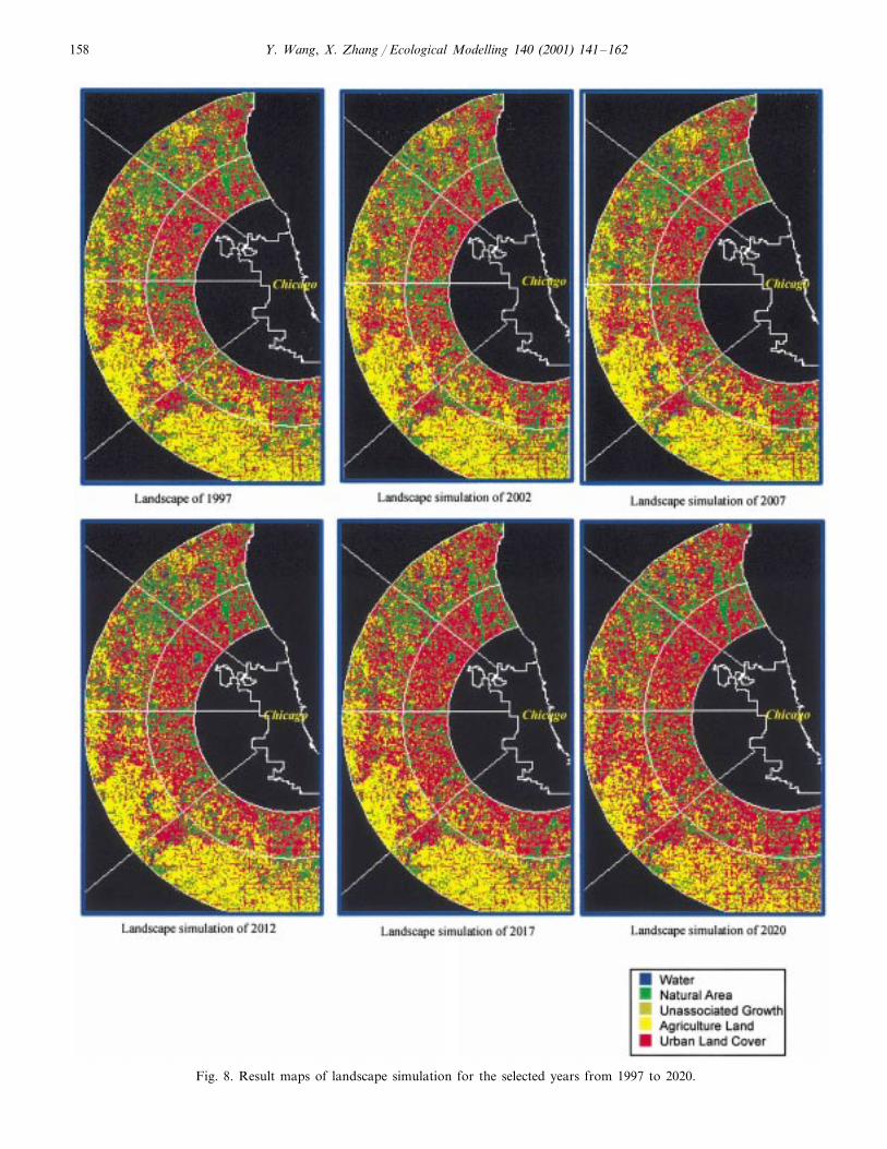
above factors on the landscape change. The land-scape simulations for the years of2002, 2007, 2012, 2017, and 2020 were achieved(Fig. 8). The simulation indicates that urbangrowth is evident in the study area. Most agricul-ture land will be converted into urban land usesby the year 2020. Natural areas tend to be moreisolated and surrounded by urban land. The trendof urbanization is predominant particularly forthe sections 5, 6, 7, 8 (Fig. 9). Increases in meanpatch size, total area, and standard deviation ofurban land are evident for all the sections afteryear 2012.

The comparison of landscape indices amongnatural and urban areas in 1985, 1997, 2012, and2020 shows that the total area, the patch density,and the mean patch size of natural areas are in adecreasing trend for all of the sections. The pat-terns of the patch density and the total areaindicate that a major decline of natural areasoccurred in sections 1, 2, 3, 4, and 5 between 1985and 1997. The same trend is continued but at areduced rate from 1997 to 2020. The lower patchdensity and smaller mean size indicate that thenatural areas in these sections are tending to bemore fragmented.

The urban growth increases the number of in-terfaces between natural and urban landscapes.We used the proportion of interface-edge betweentwo land cover types to characterize the landscapechange. The proportions of interface-edge amongland cover types show that interface edges sharedby natural and urban areas increased from 0.354in 1972, to 0.368 in 1985, to 0.492 in 1997 (Table6). The simulated results indicate that the increas-ing trends of interface-edge between natural andurban areas will continue and reach 0.524 in 2012and 0.576 in 2020, respectively. The increasingtrend of proportion of interface-edge by urbanand unassociated growth areas has been observedas well. However, the values of the proportion ofinterface-edge between natural and unassociatedgrowth areas, and between natural and agricul-tural areas, are in decreasing trends, mainlycaused by consumption of unassociated growthareas and agricultural lands by urban land uses.Although the decrease of patch density and meanpatch size of natural areas is not overwhelming

(Fig. 9), the changing pattern of the proportionsof interface-edge reflects the impacts of humanfactors on natural areas in the region.

Visual comparison between the patterns of theland covers simulated by the DLS and compiledby the Openlands Project (Openlands, 1999)shows a good match between the two. The Open-lands project predicted urban land expansion ofthe region from year 1998 to 2028 by the informa-tion about likely future land patterns obtainedthrough a series of meetings with policy makers,professional planners, open space advocates,builders and developers. Many policy and plan-ning factors, such as sewer-service expansions,highway extensions, and other future infrastruc-ture improvements, were considered. Althoughthe results of the Openlands project were mostlybased on the data from qualitative analysis andextensive interviews, the base map upon which theOpenlands project findings rooted had been cor-rected and updated by the most up-to-date devel-opment information. Various factors causingdevelopment pressures and whether areas wouldlikely develop in the short term (within 10 years)or the long term (from 10 to 30 years) were givenfull consideration (Openlands, 1999). Visual com-parison confirmed that the DLS simulation cap-tured dynamic features of human-inducedlandscape changes. Since the Openlands projectwas not GIS-based, no quantitative comparisonor measurements between the DLS and Open-lands results were attempted.

4. Discussions and conclusions

The DLS approach is designed to integrateurban spatial growth and land-cover change sub-models in simulating human-induced landscapechange. This integration allows a dynamic adjust-ment of transition structures during the simula-tion process. The adjustment overcomes theshortcomings of using a fixed or a constant transi-tion rate. Since human-induced landscape changesare closely related to socioeconomic factors, thisadjustment is critical to reflect the spatio-temporalunevenness of human impacts in dynamic model-ing. In order to represent the impact, socioeco-


Fig. 8. Result maps of landscape simulation for the selected years from 1997 to 2020.


Fig. 9. Comparison of landscape characters by DLS simulated landscape data.

nomic and demographic influences must betreated as internal components of the model. TheDLS approach explores a mechanism that can be

used to quantify and incorporate human impactson landscape dynamics. The utility function ofspatial choice allows economic principles to be


incorporated into landscape simulation. Althoughonly six socioeconomic and demographic at-tributes were discussed in this study, the method-ology enables the effects of other attributes to bedirectly linked with the simulation modeling. Themethodology in the construction of a utility func-tion creates a new paradigm for building a quanti-tative model of spatial choice.

Space available for urban land expansion isimplicit in DLS, when modeling the spatial de-mand of urban land and spatial choice of com-partments. Spatial restrictions enforced by GISdata can be effectively referenced to limit theareas of available land for urban expansion. Landavailability and dynamic change of the attributeswithin compartments for each time interval,reflect the spatial supply for urban land and ad-

just the spatial choice of compartment by theeffective population for the next time interval.

Multiple spatial units facilitate the interactionsamong the submodels. The sections allow multipletransition structures to be implemented so thatthe spatial variance of landscape changesthroughout the study area can be represented.This is important particularly when the simulationcovers a large area that has unbalanced transitionstructures and uneven development patterns.

The compartments control spatial scale of ur-ban growth simulation. Compartments adjusttransition structures of the sections by dynamicallocation of the effective population. This is thekey to incorporate socioeconomic and demo-graphic data into the landscape simulation.Whether the size of the compartment would affect

Table 6Proportion of interface-edge among land-cover types from 1972 to 1997 and for the simulated years

AgricultureUnassociated growthNatureLand cover category Urban

Proportion of interface-edge (1972)0.495Nature 0.3540.150

0.255 0.450 0.295Unassociated growth0.399 0.214 0.387Agriculture0.351 0.476Urban 0.173

Proportion of interface-edge (1985)Nature 0.3680.3090.323

0.290 0.4000.310Unassociated growthAgriculture 0.3060.312 0.382

0.310 0.359Urban 0.325

Proportion of interface-edge (1997)0.1910.316 0.492Nature

0.256Unassociated Growth 0.267 0.476Agriculture 0.189 0.326 0.484

0.314Urban 0.374 0.312

Proportion of interface-edge (2012)0.277 0.199 0.524Nature

0.230Unassociated Growth 0.259 0.510Agriculture 0.189 0.294 0.518

0.312Urban 0.3250.363

Proportion of interface-edge (2020)0.231Nature 0.193 0.576

Unassociated growth 0.5570.2440.1990.2580.177Agriculture 0.565

0.313Urban 0.350 0.337


the simulation result has not been examined yet.It was observed, however, that most of the munic-ipalities in the outer ring areas (�45 km fromdowntown Chicago) are relatively small in sizeand had been expanded dramatically in the past10 years by the annexation of the surroundingavailable lands. These municipalities have greaterpotentials to be further expanded. Therefore, thepolicy of land annexation in northeastern Illinois,as one of the driving factors, can be incorporatedinto the DLS to improve modeling performance.

The cells, with finer spatial scale, control thespatial step of land-cover simulation. The cell sizewas designed to bridge the size of a Landsat TMpixel and the spatial scale of the compartment.The cells will facilitate the integration of remotesensing data and the derivatives of land coverwith data from other sources. Although the cell isthe minimum spatial unit, land-cover type foreach of the TM pixels provides sub-cell informa-tion that can be applied to refine land coversimulation. Finer resolution of spatio-temporaldata in both socioeconomic and biophysical cate-gories should improve and enhance the capacityof the model.

The results of this DLS modeling are particu-larly telling in the case of one of the most severethreats to the region’s environment: urban sprawland its consequences. The simulated landscapesreveal a dramatic trend in urban land increase.Fragmentation and isolation of the natural com-munities are evident in the study area andthroughout the region. Even though most of theregion’s high quality natural areas are in conser-vation management and more open lands will beprotected, the integrity and viability of naturalecosystems will be altered by the accelerated tran-sition of surrounding agricultural land to urbanstructures. The pattern of sprawling growth in theChicago region has been recognized by the con-cerned agencies. Region-wide planning efforts, asaddressed in the latest regional Biodiversity Re-covery Plan (Chicago Wilderness, 1999), are un-derway. The DLS approach provides a newprototype for this type of regional study. Thesimulation results are helpful in understanding thecurrent and future landscape patterns and in man-agement planning.

Acknowledgements

We are very grateful to Dr Jianguo Liu ofMichigan State University for his detailed adviceon improvement of the manuscript. We thank theanonymous reviewers for their insights and criti-cal review of the manuscript. This research wassupported by National Aeronautics and SpaceAdministration grants GP37J and NAG5-8829.The land-cover change detection project (NASAGrant GP37J), upon which the land cover datacame from, was the collaborative effort of anenormous group of ecologists and land managersin the Chicago metropolitan region and ChicagoWilderness. We thank all of them, in particularDebra Moskovits, Stephen Packard, WayneLampa, and Wayne Schennum, for their expertiseand insights. We also thank Professor CliffordTiedemann of the University of Illinois atChicago for his editorial comments on themanuscript.

References

Boerner, R.E.J., DeMers, M.N., Simpson, J.W., Artigas, F.J.,Silva, A., Berns, L.A., 1996. Markov Models of inertia anddynamic on two contiguous Ohio landscapes. Geographi-cal Analysis 28, 56–66.

Chicago Wilderness, 1999. Biodiversity Recovery Plan,Chicago Wilderness, Chicago, pp. 18–26.

Childress, W.M., 1997. Predicting dynamics of spatial au-tomata models using Hamiltonian equations. EcologicalModelling 96, 293–303.

Clarke, K.C., Gaydos, L.J., 1998. Long term urban growthprediction using a cellular automaton model and GIS:Applications in San Franciso and Washington/Baltimore.International Journal of Geographical Information Science12, 699–714.

Dunn, C.P., Sharpe, D.M., Guntenspergen, G.R., Steams, F.,Yang, Z., 1990. Methods for analyzing temporal changesin landscape pattern. In: Turner, M.G., Gardner, R.H.(Eds.), Quantitative Methods in Landscape Ecology.Springer, New York, pp. 173–198.

Ehrlich, P.R., 1988. The loss of diversity: cause and conse-quences. In: Wilson, E.O. (Ed.), Biodiversity. NationalAcademy Press, Washington, DC, pp. 21–27.

Flamm, R.O., Turner, M.G., 1994. Alternative model formu-lations for a stochastic simulation of landscape change.Landscape Ecology 9, 37–46.

Gardner, R.H., Milne, B.T., Turner, M.G., O’Neill, R.V.,1987. Natural models for the analysis of broad-scale land-scape pattern. Landscape Ecology 1, 19–28.


Hall, F.G, Strebel, D.E., Sellers, P.J., 1988. Linking knowl-edge among spatial and temporal scales: vegetation, atmo-sphere, climate and remote sensing. Landscape Ecology 2,3–22.

Jensen, J.R., Cowen, D.J., Halls, J., Narumalani, S., Schmidt,N.J., Davis, B.A., Burgess, B., 1994. Improved urbaninfrastructure mapping and forecasting for Bellsouth usingremote sensing and GIS technology. Photogrammetric En-gineering and Remote Sensing 60, 339–346.

Leonardi, G., Papageorgiou, Y.Y., 1992. Conceptual founda-tion of spatial choice models. Environment and PlanningA24, 1393–1408.

Li, H., Reynolds, J.F., 1997. Modeling effects of spatial pat-tern, drought, and grazing on rates of rangeland degrada-tion: a combined Markov and cellular automatonapproach. In: Quattrochi, D.A., Goodchild, M.F. (Eds.),Scale in Remote Sensing and GIS. Lewis Publishers, BocaRaton, Florida, pp. 211–230.

Liu, J., Ashton, P.S., 1998. FORMOSAIC: an individual-based spatially explicit model for simulating forest dynam-ics in landscape mosaics. Ecological Modelling 106,177–200.

Lo, C.P., Faber, B.J., 1997. Integration of Landsat thematicmapper and census data for quality of life assessment.Remote Sensing of Environment 62, 143–157.

Mansfield, E., 1982. Micro-Economics: Theory & Applica-tions. W.W. Norton and Company, Inc., New York, pp.57–63.

Muller, M.R., Middleton, J., 1994. A Markov model of land-use change dynamics in the Niagara Region, Ontario,Canada. Landscape Ecology 9, 151–157.

NIPC, 1998. Population, household and employment forecastsfor northeastern Illinois 1990 to 2020. Northeastern IllinoisPlanning Commission, Chicago, pp. 1–25.

O’Neill, R.V., Krummel, J.R., Gardner, R.H., Sugihari, G.,Jackson, B., DeAngelis, D.L., Milne, B.T., Turner, M.G.,Zygmunt, G., Christensen, S.W., Dale, V.H., Graham,R.L., 1988. Indices of landscape pattern. Landscape Ecol-ogy 3, 153–162.

O’Neill, R.V., Johnson, A.R., King, A.W., 1989. A hierarchi-

cal framework for the analysis of scale. Landscape Ecology3, 193–205.

Openlands Project, 1999. Under Pressure: Land Consumptionin the Chicago Region 1998–2028. Openlands Project,Chicago, pp. 1–31.

Parrot, R., Stutz, F.P., 1991. Urban GIS application. In:Maguire, D.J., Goodchild, M.F., Rhind, D.W. (Eds.), Ge-ographical Information Systems: Principles And Applica-tion. Longman, London, pp. 247–260.

Peterson, W., 1989. Principles of Economics: Micro. RichardD. Irwin, Inc, Homewood, Illinois, pp. 37–43.

Sher, W., Pinola, R., 1981. Microeconomic Theory: A Synthe-sis of Classical Theory and the Modern Approach. ElsevierNorth Holland, Inc, New York, pp. 185–191.

Silvertown, J., Holtier, S., Johnson, J., Dale, P., 1992. Cellularautomaton models of interspecific competition for space-the effect of pattern on process. Journal of Ecology 80,527–534.

Timmerman, H., Borgers, A., 1989. Dynamic models of choicebehavior: some fundamentals and trends. In: Hauer, J.(Ed.), Urban Dynamics and Spatial Choice Behavior.Kluwer Academic Publishers, pp. 3–26.

Turner, M.G., 1987. Spatial simulation of landscape changesin Georgia: a comparison of three transition models. Land-scape Ecology 1, 29–36.

Turner, M.G., Costanza, R., Sklar, F.H., 1989. Methods toevaluate the performance of spatial simulation models.Ecological Modelling 48, 1–18.

Wu, F., 1998. SimLand: a prototype to simulate land conver-sion through the integrated GIS and CA with AHP-derivedtransition rules. International Journal of Geographical In-formation Sciences 12, 63–82.

Xie, Y., 1996. A generalized model for cellular urban dynam-ics. Geographical Analysis 28, 350–373.

Zhang, X., He, J., 1997. Urban spatial growth and spatio-tem-poral pattern of urban land development. Journal of Re-mote Sensing 1, 145–151 in Chinese with English abstract.

Zhou, G., Liebhold, A.M., 1995. Forecasting the spread ofgypsy moth outbreaks using cellular transition models.Landscape Ecology 10, 177–186.

.

Documents

A dynamic modeling approach to simulating socioeconomic ...csr.ufmg.br/modelagem_sistemas_dinamicos/wang_urban_dynamics.pdf · Ecological Modelling 140 (2001) 141–162 A dynamic