Embed Size (px)
Citation preview

Center for Analytical Finance University of California, Santa Cruz
Working Paper No. 34
A Dynamic Model of Firm Valuation
Natalia Lazzati a, Amilcar A. Menichini b
aDepartment of Economics, University of California, Santa Cruz, [email protected] b Graduate School of Business and Public Policy, Naval Postgraduate School, Monterey, California, [email protected]
September 2016
Abstract
We propose a dynamic version of the dividend discount model, solve it in closed-form, and assess its empirical validity. The valuation method is tractable and can be easily implemented. We find that our model produces equity value forecasts that are, on average, very close to market prices, and explains a large proportion (around 83%) of the observed variation in share prices. Moreover, we find that a simple portfolio strategy based on the difference between market and estimated values earns considerably positive returns, on average. These returns are uncorrelated with the three risk factors in Fama and French (1993). Keywords: Firm Valuation; Dividend Discount Model; Gordon Growth Model; Dynamic Programming. JEL Codes: G31, G32. About CAFIN The Center for Analytical Finance (CAFIN) includes a global network of researchers whose aim is to produce cutting edge research with practical applications in the area of finance and financial markets. CAFIN focuses primarily on three critical areas:
• Market Design • Systemic Risk • Financial Access
Seed funding for CAFIN has been provided by Dean Sheldon Kamieniecki of the Division of Social Sciences at the University of California, Santa Cruz.

A Dynamic Model of Firm Valuation
Natalia Lazzati and Amilcar A. Menichini∗
September, 2016
Abstract
We propose a dynamic version of the dividend discount model, solve it in closed-form, and
assess its empirical validity. The valuation method is tractable and can be easily implemented.
We find that our model produces equity value forecasts that are, on average, very close to
market prices, and explains a large proportion (around 83%) of the observed variation in share
prices. Moreover, we find that a simple portfolio strategy based on the difference between
market and estimated values earns considerably positive returns, on average. These returns
are uncorrelated with the three risk factors in Fama and French (1993).
JEL classification: G31, G32
Keywords: Firm Valuation; Dividend Discount Model; Gordon Growth Model; Dynamic Pro-
gramming
∗Natalia Lazzati is from the Department of Economics, UC Santa Cruz, CA 95064 (e-mail: [email protected]).
Amilcar A. Menichini is from the Graduate School of Business and Public Policy, Naval Postgraduate School,
Monterey, CA 93943 (e-mail: [email protected]). We thank the financial support from the Center for Analytical
Finance (CAFIN) at UC Santa Cruz, as well as the research assistance of Luka Kocic. We also thank the helpful
comments from Chris Lamoureux and Scott Cederburg.
1
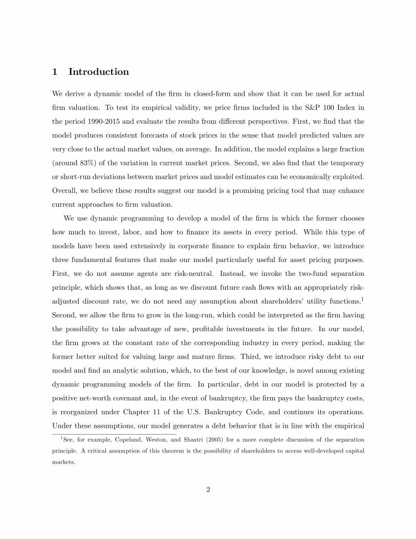
1 Introduction
We derive a dynamic model of the firm in closed-form and show that it can be used for actual
firm valuation. To test its empirical validity, we price firms included in the S&P 100 Index in
the period 1990-2015 and evaluate the results from different perspectives. First, we find that the
model produces consistent forecasts of stock prices in the sense that model predicted values are
very close to the actual market values, on average. In addition, the model explains a large fraction
(around 83%) of the variation in current market prices. Second, we also find that the temporary
or short-run deviations between market prices and model estimates can be economically exploited.
Overall, we believe these results suggest our model is a promising pricing tool that may enhance
current approaches to firm valuation.
We use dynamic programming to develop a model of the firm in which the former chooses
how much to invest, labor, and how to finance its assets in every period. While this type of
models have been used extensively in corporate finance to explain firm behavior, we introduce
three fundamental features that make our model particularly useful for asset pricing purposes.
First, we do not assume agents are risk-neutral. Instead, we invoke the two-fund separation
principle, which shows that, as long as we discount future cash flows with an appropriately risk-
adjusted discount rate, we do not need any assumption about shareholders’utility functions.1
Second, we allow the firm to grow in the long-run, which could be interpreted as the firm having
the possibility to take advantage of new, profitable investments in the future. In our model,
the firm grows at the constant rate of the corresponding industry in every period, making the
former better suited for valuing large and mature firms. Third, we introduce risky debt to our
model and find an analytic solution, which, to the best of our knowledge, is novel among existing
dynamic programming models of the firm. In particular, debt in our model is protected by a
positive net-worth covenant and, in the event of bankruptcy, the firm pays the bankruptcy costs,
is reorganized under Chapter 11 of the U.S. Bankruptcy Code, and continues its operations.
Under these assumptions, our model generates a debt behavior that is in line with the empirical
1See, for example, Copeland, Weston, and Shastri (2005) for a more complete discussion of the separation
principle. A critical assumption of this theorem is the possibility of shareholders to access well-developed capital
markets.
2

evidence. For instance, survey results from Graham and Harvey (2001) suggest that most firms
have a target leverage. Consistently, the firm in our model chooses debt in every period following
a target leverage that depends on its own characteristics.
As mentioned above, an important advantage of our model regarding valuation is that we
solve it analytically. Closed-form equations are strongly preferred to numerical approximations
because the former yield extremely accurate values at very low computing time. Indeed, a usual
problem with the numerical solution of dynamic programming models is the so-called Bellman’s
curse of dimensionality. This problem arises from the discretization of continuous state and
decision variables, since the computer time and space needed increases exponentially with the
number of points in the discretization (Rust, 1997, 2008). Thus, more accurate firm valuations
imply necessarily exponentially longer periods of computing time. In addition, explicit solutions
allow the user to estimate model parameters with ease.
We start analyzing the performance of our model by doing a comparative statics analysis of
the stock price with respect to all model parameters. We find that share price is more sensitive
with respect to the operating aspects of the firm (e.g., the curvature of the production function
and the persistence of profit shocks). This information helps the user to, for instance, ascertain
which parameters require greater attention in the estimation step. We then proceed to study
the actual pricing performance of the model with firms that were included in the S&P 100 Index
in the period 1990-2015. We first compute the ratio of the actual market prices to the values
predicted by our model and its mean value turns out to be around 1. This result suggests that
our model yields equity value estimates that are, on average, very close to market values. We
then regress the market value of equity on the value estimated by our model and find that the
latter can explain a large fraction of the observed variability of the former (around 83%). This
outcome turns out to be better than the results reported by related papers (described below),
and implies a strong linkage between model implied and market values over time.2
While we show that our estimates are, on average, very close to market values, we also
2Complementing the results in this article, Lazzati and Menichini (2015b) show that a simpler version of
this model also explains numerous important regularities documented by the empirical literature in corporate
finance. For instance, it rationalizes the negative association between profitability and leverage, the existence and
characteristics of all-equity firms, and the inverse relation between dividends and investment-cash flow sensitivities.
3

find temporary deviations between stock prices and model estimates. We then implement simple
portfolio strategies to test whether we can take advantage of those deviations. The former consist
in ranking firms based on their ratios of market prices to model estimates, then forming quintile
portfolios based on those ratios, and finally buying the firms in the lowest quintile portfolio and
selling the firms in the highest quintile portfolio. Our results show that those strategies earn,
on average, around 21%, 36%, and 52% returns after one, two, and three years of portfolio
formation, respectively. We also study whether those returns can be explained by the three risk
factors described by Fama and French (1993), but find that they are uncorrelated with the latter.
As benchmark, we calculate the returns of portfolios constructed according to two well-known
ratios: market-to-book and price-earnings. We find that the former yields around 13%, 19%, and
30% returns after one, two, and three years of portfolio formation, while the latter yields 8%, 14%,
and 20% returns in the same periods. That is, our portfolio strategy consistently outperforms
those based on the market-to-book and price-earnings ratios.
To do the previous analyses, we use the simulated method of moments to estimate the struc-
tural parameters for firms included in the S&P 100 Index during the period 1990-2015. This
procedure estimates parameters by minimizing the distance between certain moments computed
from the data and the same moments simulated with the model.3 In all our estimations, we
perform a forward-looking exercise in the sense that we use data available prior to the valuation
period to make out-of-sample predictions. Doing so is important because this procedure replicates
the situation a user would face when performing actual valuation.
Finally, we should also mention that we valuated firms included in the S&P 100 Index in
order to assess the empirical performance of our model. However, our valuation model can be
implemented with firms for which market prices do not exist, as long as financial statements are
available for parameter estimation. These cases include, among others, private companies such
as Koch Industries and Cargill, IPOs such as Facebook in 2012 and Alibaba Group Holding in
2014, and firms’new investment projects.
3The simulated method of moments is analyzed theoretically in Gourieroux, Monfort, and Renault (1993) and
Gourieroux and Monfort (1996). Strebulaev and Whited (2012) contains a detailed description of its implementa-
tion.
4

Literature Review
Our paper contributes to two different strands of literature in finance, namely, dynamic pro-
gramming models of the firm and firm valuation models.
Several papers in corporate finance use different dynamic programming models of the firm
to explain firm choices. For instance, Moyen (2004, 2007), Hennessy and Whited (2005, 2007),
Hennessy, Levy, and Whited (2007), Tserlukevich (2008), Riddick and Whited (2009), and Hen-
nessy, Livdan, and Miranda (2010), among others, use those models to rationalize a large number
of stylized facts about firm behavior.4 We show that – after introducing some new features–
this type of models can also be used successfully for firm valuation. As we mentioned before, we
get rid of any specification of shareholders’utility function by assuming the two-fund separation
principle. In the context of the latter, as long as we discount future cash flows with market
discount rates, we can disregard the risk-neutrality assumption. This possibility was suggested
by Dixit and Pindyck (1994) and we believe our paper is one of the first attempts in this direc-
tion. Another important feature regarding valuation is the possibility of the firm to grow in the
long-run. As documented by Lazzati and Menichini (2015a), secular growth can account for more
than 30% of the value of the firm, and it is of particular importance for certain industries, such as
manufacturers of chemical products and industrial machinery, and providers of communication
services (Jorgenson and Stiroh, 2000). In addition, as we explained before, the fact that we obtain
closed-form solutions is very important for the accuracy of the model predictions.
While we show in this paper that our model produces successful valuation results, we also
find that it performs similarly in some regards and better in some others when compared to
other valuation models. We obtain similar results to those of Kaplan and Ruback (1995) and
Copeland, Weston, and Shastri (2005), who implement the discounted cash flow model (DCFM)
and show that it produces value forecasts that are, as in our case, roughly equal to market
prices. With respect to the explanation of the variation in current market prices, our model
seems to outperform the results in some related studies: Bernard (1995) compares the ability
of the dividend discount model (DDM) and the residual income model (RIM) to explain the
observed variation in stock prices. He finds that the RIM explains 68% of the variability in
4See Strebulaev and Whited (2012) for a comprehensive review of this literature.
5

market values and outperforms the DDM, which can only explain 29% of such variation.5 In a
similar study, Frankel and Lee (1998) test the RIM empirically and find that the model estimates
explain around 67% of the variability in current stock prices. More recently, Spiegel and Tookes
(2013) use a dynamic model of oligopolistic competition to perform cross-sectional valuation and
find that their model explains around 43% of the variation in market values. Compared to these
papers, we find that our model can explain a higher fraction of the variability of the stock prices
(around 83%).6
The paper is organized as follows. In Section 2, we derive a dynamic version of the DDM
in closed-form and explain its main parts. Section 3 contains the sensitivity analysis of the
stock price with respect to the different firm characteristics. The empirical evaluation of the
performance of our model is in Section 4. Section 5 concludes. Appendix 1 contains the proofs.
2 A Dynamic Dividend Discount Model
In this section, we derive a dynamic version of the standard DDM in closed-form. We solve
the problem of the firm (i.e., share price maximization) using discrete-time, infinite-horizon,
stochastic dynamic programming. The solution is obtained within the context of the Adjusted
Present Value (APV) method introduced by Myers (1974), which has been used extensively with
dynamic models of the firm (e.g., Leland, 1994; Goldstein, Ju, and Leland, 2001; and Strebulaev,
2007).7
2.1 The Problem of the Firm
The life horizon of the firm is infinite, which implies that shareholders believe it will run
forever. The CEO makes investment, labor, and financing decisions at the end of every time
5The DDM, the DCFM, and the RIM are theoretically equivalent, but they differ with respect to the information
used in their practical implementation. The DDM uses the future stream of expected dividend payments to
shareholders. The DCFM is based on some measure of future cash flows, such as free cash flows. Finally, the RIM
uses accounting data (e.g., current and future book value of equity and earnings).6 In all those papers, the samples differ in terms of firm composition and time periods.7As it is common with other valuation models (e.g., the Black-Scholes formula), we do not introduce transaction
or adjustment costs to our model.
6

period (e.g., month, quarter, or year) such that the market value of equity is maximized. (In this
paper, we write a tilde on X (i.e., X) to indicate that the variable is growing over time.) Variable
Kt represents the book value of assets while variable Lt indicates the amount of labor used by
the firm in period t. In each period, installed capital depreciates at constant rate δ > 0.
The debt of the firm in period t, Dt, matures in one period and is rolled over at the end of
every period. We assume debt is issued at par by letting the coupon rate cB equal the market
cost of debt rB. In turn, this feature implies that book value of debt Dt equals the market value
of debt Bt. The amount of outstanding debt Bt will increase or decrease over time according
to financing decisions. We let debt be risky, which implies that the firm goes into bankruptcy
when profits are suffi ciently low (e.g., negative). Following Brennan and Schwartz (1984), we
assume the debt contract includes a protective covenant consisting of a weakly positive net-worth
restriction. According to that covenant, in order to avoid bankruptcy, the book value of equity
must be weakly positive. In the event of bankruptcy, the firm has to pay bankruptcy costs ξKt
(with ξ > 0), such as lawyer fees and other costs of the bankruptcy proceedings. Furthermore, we
assume the bankrupt firm is reorganized and continues its operations after filing for protection
under Chapter 11 of the U.S. Bankruptcy Code. This assumption is consistent with the empirical
evidence showing that the majority of firms emerge from Chapter 11 and only few are actually
liquidated under Chapter 7 (see, e.g., Morse and Shaw, 1988; Weiss, 1990; and Gilson, John and
Lang, 1990). Finally, as in Hennessy and Whited (2007), we let those costs be proportional to
the level of assets.
We introduce randomness into the model through the profit shock zt. Following Fama and
French (2000), we let profits be mean-reverting by assuming that random shocks follow an AR(1)
process in logs
ln (zt) = ln (c) + ρ ln (zt−1) + σxt (1)
where ρ ∈ (0, 1) is the autoregressive parameter that defines the persistence of profit shocks. In
other words, a high ρ makes periods of high profit innovations (e.g., economic expansions) and
low profit shocks (e.g., recessions) last more on average, and vice versa. The innovation term
xt is assumed to be an iid standard normal random variable, scaled by constant σ > 0. The
latter defines the volatility of profits over time. Finally, constant c > 0 defines the mean value
7

toward which random shocks revert (i.e., E [ln (zt)] = ln (c) / (1− ρ)). Thus, this parameter has a
direct impact on expected profits and an important influence on the current size of the firm. This
parameter is important because it helps to capture unobserved firm-specific features affecting
firm profitability and are not explained by either ρ or σ. It is common in the corporate finance
literature to normalize c to 1, which allows for the study of representative firms. However, that
assumption undermines the valuation attempt as the estimated prices may result strongly biased.
Given that our objective is to evaluate the pricing performance of our model with actual data,
we do not do such normalization and use our modeling restrictions to recover the value of c for
each firm.
Gross profits in period t are defined by the following function
Qt = (1 + g)t[1−(αK+αL)] ztKαKt LαLt (2)
where zt is the profit shock in period t, αK ∈ (0, 1) represents the elasticity of capital, and
αL ∈ (0, 1) indicates the elasticity of labor (we further assume αK + αL < 1). Constant g
represents the growth rate of the industry to which the firm belongs and, with this factor, profits,
costs and firm size grow proportionately over time.8 Caves (1998) finds that firm growth becomes
less volatile over time as the firm becomes large. Therefore, our restriction makes the model better
suited for pricing lower growth firms, such as the large and mature corporations we value in this
article (i.e., firms in the S&P 100 Index). Equation (2) says that gross profits also depend on a
Cobb-Douglas production function with decreasing returns to scale in capital and labor inputs.9
Every period, the firm pays operating costs fKt (with f > 0) and labor wages ωLt (with
ω > 0), while corporate earnings are taxed at rate τ ∈ (0, 1). Therefore, the firm’s net profits in
period t are
Nt =(Qt − fKt − δKt − ωLt − rBBt
)(1− τ) . (3)
With all the previous information, we can state the cash flow that the firm pays to equity-holders
8Factor (1 + g)t[1−(αK+αL)] allows us to use a standard normalization of growing variables that is required to
solve the problem of the firm (see, e.g., Manzano, Perez, and Ruiz, 2005).9Equation (2) can take on only (weakly) positive values. However, the model can be easily extended to allow for
negative values of gross profits by subtracting a positive constant as a proportion of assets (e.g., aKt) in equation
(2).
8

in period t as
Yt = Nt −[(Kt+1 − Kt
)−(Bt+1 − Bt
)]−ΘξKt. (4)
According to equation (4), the dividend paid to shareholders in period t equals net profits minus
the change in equity and, in the event of bankruptcy (i.e., Θ = 1), minus the bankruptcy costs.
We let rate rS represent the market cost of equity and rate rA denote the market cost of capital.
We also assume the secular growth rate is lower than the market cost of capital (i.e., g < rA).
Finally, given the current state at t = 0, (K0, L0, B0, z0), the problem of the firm is to make the
optimal capital, labor, and debt decisions, such that the market value of equity is maximized.10
Before we solve the firm problem, we need to convert it into stationary, for which we normalize
the growing variables by the gross growth rate: Xt = Xt/(1+g)t, withXt = {Kt, Lt, Bt, Qt, Nt, Yt}.
We let E0 indicate the expectation operator given information at t = 0. Using the normalized
variables and modifying the payoff function accordingly, the market value of equity can be ex-
pressed as
S (K0, L0, B0, z0) = max{Kt+1,Lt+1,Bt+1}∞t=0
E0
∞∑t=0
(1 + g)t∏tj=0
(1 + rSj
)Yt. (5)
We solve that problem by separating investment (and labor) from financing decisions, as shown
by Modigliani and Miller (1958). This separation is possible in our dynamic model because debt
is a static decision (i.e., it can be fully adjusted in each period of time).
2.2 Model Solution
To help streamline the exposition, we solve the problem of the firm – equation (5)– in
Appendix 1. We find the following closed-forms for the stock price when the firm does not go
into bankruptcy. As a by-product, we also characterize the probability of bankruptcy and the
optimal leverage ratio analytically.
Proposition 1 The market value of equity is
S (Kt, Lt, Bt, zt) = [ztKαKt LαLt − fKt − δKt − ωLt − rBBt] (1− τ) +
Kt −Bt +G (zt)(6)
10The restriction(f + δ + ω
Φ∗2
Φ∗1
)(1− τ) + ξ ≤ 1 guarantees that both debt and firm value are weakly positive.
9

where the going concern value is Gt (zt) = M (zt)P∗. Variable M (zt) is given by
M (zt) = e− 1
2σ2 (αK+αL)
[1−(αK+αL)]2{(
1+g1+rA
)E[z
1/[1−(αK+αL)]t+1 |zt
]+(
1+g1+rA
)2E[z
1/[1−(αK+αL)]t+2 |zt
]+ ...
} (7)
with the general term
E[z
1/[1−(αK+αL)]t+n |zt
]=
c 1−ρn1−ρ zρ
n
t e12σ2 (1−ρ2n)
(1−ρ2)1
[1−(αK+αL)]
11−(αK+αL)
, n = 1, 2, ... (8)
and variable P ∗ takes the form
P ∗ =(Φ∗
αK
1 Φ∗αL
2 − fΦ∗1 − δΦ∗1 − ωΦ∗2)
(1− τ)− rAΦ∗1 +
(1 + rA1 + rB
)(rBτ`
∗ − λ∗ξ) Φ∗1 (9)
with
Φ∗1 =
( αKrA
1−τ + f + δ
)1−αL (αLω
)αL 11−(αK+αL)
(10)
and
Φ∗2 =
[(αK
rA1−τ + f + δ
)αK (αLω
)1−αK] 1
1−(αK+αL)
. (11)
The probability of bankruptcy is
λ∗ =
∫ x∗c
−∞
1√2πe−
z2
2 dz (12)
where
x∗c = −σ −
√√√√√2
σ2 + ln
[1 + 1
rB(1−τ)
]ξ
√2πτσΦ∗αK−1
1 Φ∗αL2
. (13)
The optimal book leverage ratio is given by
`∗ =1 +
[eσ(x
∗c− 1
2σ)Φ∗αK−1
1 Φ∗αL2 − f − δ − ωΦ∗2Φ∗1
](1− τ)− ξ
1 + rB (1− τ)(14)
The market value of equity is shown in equation (6) and represents an analytic solution of
the Gordon Growth Model (Gordon, 1962) in the dynamic and stochastic setting. The first three
terms in equation (6) represent the after-shock book value of equity, while the last term, G (zt), is
the going-concern value. The latter depends on variable M (zt), which captures the effect of the
10

infinite sequence of expected profit shocks, and on variable P ∗, which denotes the dollar return
on capital minus the dollar cost of capital at the optimum (including the interest tax shields
and bankruptcy costs as financing side effects).11 The going-concern value shows that, using
only information about the current state (i.e., assets, labor, debt, and gross profits), our model
solves systematically for the full sequence of expected future dividends. Our model also projects
automatically the value of the real options (such as the option to expand the business, extend
the life of current projects, shrink the firm, or even postpone investments) by allowing the firm
to optimize decisions over time.12
Optimal capital turns out to be K∗ (zt) = (1 + g)E [zt+1|zt]1
1−(αK+αL) Φ∗1, which shows how
the former depends on the primitive firm characteristics. As expected, it decreases with the
market cost of capital rA, operating costs f , depreciation δ, and labor costs ω. On the contrary,
optimal assets increase with the growth rate g, constant c, and the volatility of innovations σ
because they increment the expected profitability of capital via equation (3). The effects of
αK , αL, and ρ depend on current profit shock zt, but they are generally positive for standard
values of the parameters. Optimal labor has the form L∗ (zt) = (1 + g)E [zt+1|zt]1
1−(αK+αL) Φ∗2,
and its sensitivity with respect to the fundamental characteristics of the firm is analogous too that
of optimal assets. Optimal debt is B∗ (zt) = `∗K∗ (zt) and all the previous characteristics have
the same directional effects on this decision. Finally, the income tax rate τ has a negative effect
on optimal assets and labor because the latter become less profitable as the former is higher. It
also has a negative effect on optimal debt for the great majority of parameter values, including
those used in this paper.
In a survey, Graham and Harvey (2001) provide empirical evidence suggesting that most firms
actually follow some form of target leverage. Consistently, our model produces an optimal debt
that is a constant proportion of optimal assets, with the factor of proportionality given by `∗
in equation (14). This optimal ratio can be interpreted as the target leverage of the firm. It is
11Function M (zt) suggests that our model can become an n-stage dynamic DDM if we substitute the growth
rate g on the numerator of the discount factor appropriately.12 In a simpler version of this model, Lazzati and Menichini (2015a) show that the value of the real options can
easily represent more than 8% of the stock price and is particularly important for certain industries, such as in Oil
and Gas Extraction. This is a further advantage of our model over static ones.
11
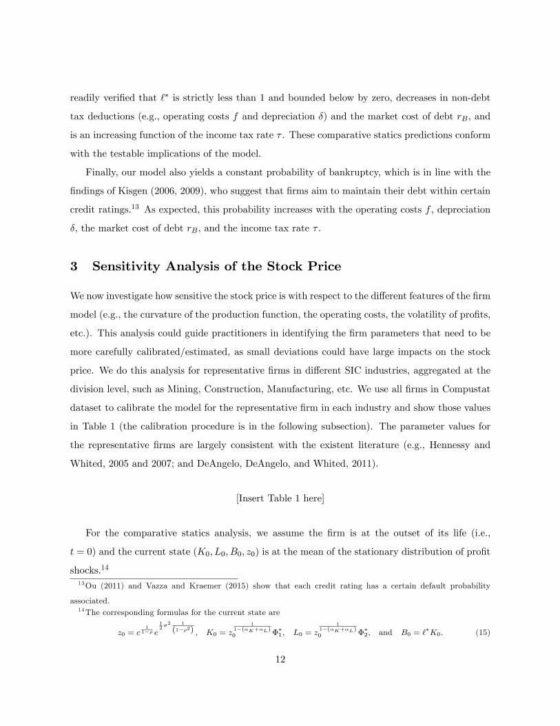
readily verified that `∗ is strictly less than 1 and bounded below by zero, decreases in non-debt
tax deductions (e.g., operating costs f and depreciation δ) and the market cost of debt rB, and
is an increasing function of the income tax rate τ . These comparative statics predictions conform
with the testable implications of the model.
Finally, our model also yields a constant probability of bankruptcy, which is in line with the
findings of Kisgen (2006, 2009), who suggest that firms aim to maintain their debt within certain
credit ratings.13 As expected, this probability increases with the operating costs f , depreciation
δ, the market cost of debt rB, and the income tax rate τ .
3 Sensitivity Analysis of the Stock Price
We now investigate how sensitive the stock price is with respect to the different features of the firm
model (e.g., the curvature of the production function, the operating costs, the volatility of profits,
etc.). This analysis could guide practitioners in identifying the firm parameters that need to be
more carefully calibrated/estimated, as small deviations could have large impacts on the stock
price. We do this analysis for representative firms in different SIC industries, aggregated at the
division level, such as Mining, Construction, Manufacturing, etc. We use all firms in Compustat
dataset to calibrate the model for the representative firm in each industry and show those values
in Table 1 (the calibration procedure is in the following subsection). The parameter values for
the representative firms are largely consistent with the existent literature (e.g., Hennessy and
Whited, 2005 and 2007; and DeAngelo, DeAngelo, and Whited, 2011).
[Insert Table 1 here]
For the comparative statics analysis, we assume the firm is at the outset of its life (i.e.,
t = 0) and the current state (K0, L0, B0, z0) is at the mean of the stationary distribution of profit
shocks.14
13Ou (2011) and Vazza and Kraemer (2015) show that each credit rating has a certain default probability
associated.14The corresponding formulas for the current state are
z0 = c1
1−ρ e
12σ2 1
(1−ρ2) , K0 = z1
1−(αK+αL)0 Φ∗1, L0 = z
11−(αK+αL)0 Φ∗2, and B0 = `∗K0. (15)
12

The sensitivity analysis of the stock price with respect to model parameter values is in Table 2.
Specifically, we show in the table the percentage change in share price when the parameter values
increase by 1%. In our model, the parameters with the highest marginal effects are the elasticity
of capital (αK) and the persistence of profit shocks (ρ). A 1% increase in these parameter values
augments the stock price between 7% and 12% across the different industries. As equation (8)
suggests, both of these parameters directly increase the expected profits of the firm and, thus,
have a substantial influence on firm size (i.e., and share price).15
Second in importance are constant c, the elasticity of labor (αL), and the market cost of
capital (rA). The impact of these parameters on the stock price is between 1% and 4% (in
absolute values) across the different industries. Equation (8) also shows that both c and αL
directly affect expected firm profitability, which explains their considerable impact on the stock
price. The (negative) impact of rA on share price is due to the strong effect of this parameter on
the discounting of future cash flows, as shown in equation (7). The remaining parameters have a
relatively small marginal effect of less than 1% (in absolute values).16
[Insert Table 2 here]
Overall, the results above suggest that the operating aspects of the firm play the most im-
portant role in the comparative statics analysis. Thus, firm primitives such as constant c, the
persistence of profit shocks (ρ), the curvature of the production function with respect to capital
(αK) and labor (αL), and the market cost of capital (rA) should be the ones that receive the
greatest attention in the calibration/estimation procedure previous to firm valuation. In addition,
richer datasets than Compustat containing more accurate information about, for instance, gross
profits and assets, could also improve the precision of the parameter estimates.
where Φ∗1, Φ∗2, and `∗ are as described in Proposition 1.
15Parameter αK has received great attention in the literature of Industrial Organization; see, e.g., Ackerberg,
Benkard, Berry, and Pakes, 2007, and the references therein.16This analysis extends Lazzati and Menichini (2015a), who perform a sensitivity analysis of the stock price for
a simpler model of the firm.
13

3.1 Calibration of Model Parameters
In this subsection, we describe how we calibrate the model parameters for the representative
firm in each SIC industry. The parameters of interest are c, ρ, σ, αK , αL, f, δ, ω, τ , rB, rA, g, and
ξ. The sample includes all firms in Compustat database and covers the period 1950-2015.
Following Moyen (2004), we obtain parameters c, ρ, σ, αK and αL using the firm’s autore-
gressive profit shock process of equation (1) and the gross profits function in equation (2). The
data we use with these equations are Gross Profit (GP), Assets - Total (AT), and Number of
Employees (EMP). We first log-linearize the gross profits function and obtain parameters αK and
αL by doing an OLS regression.17 We then use the residual term from that regression with the
firm’s autoregressive profit shock process to obtain parameters c, ρ, and σ.
We calibrate parameter f by averaging the ratio Selling, General, and Administrative Expense
(XSGA)/Assets - Total (AT) for all firm-years in each industry. We follow the same procedure
to get δ from the ratio of Depreciation and Amortization (DP) over Assets - Total (AT), ω
from the fraction Staff Expense - Total (XLR)/Number of Employees (EMP), τ from the ratio
Income Taxes - Total (TXT) over Pretax Income (PI), and rB as the proportion Interest and
Related Expense - Total (XINT)/Liabilities - Total (LT). We follow the procedure described by
Kaplan and Ruback (1995) to derive rA using CAPM after unlevering the equity beta.18 We use
the industry long-run growth rates in Jorgenson and Stiroh (2000) as parameter g for each SIC
industry. Finally, we calibrate ξ using the fraction Liabilities - Total (LT)/Assets - Total (AT) in
equation (14). We exclude firms with SIC 6000-6700 (i.e., Finance, Insurance, and Real Estate)
as well as firms with SIC 9100-9900 (i.e., Public Administration). We also eliminate observations
with missing data and trim those ratios at the lower and upper one-percentiles to reduce the
effect of outliers and errors in the data. The final sample includes 62,036 firm-year observations.
17This is a standard procedure in the empirical economics literature (see, e.g., Balistreri, McDaniel, and Wong
2003; Fox and Smeets 2011; Young 2013).18We use the market risk premiums published on Damodaran’s website, and the 10-year T-Bond yields as the
risk-free interest rate.
14

4 Testing the Performance of the Valuation Model
We finally study two fundamental aspects of our dynamic model. First, we analyze the consistency
between the model estimates and market prices. That is, we address how close the predicted values
by our model are to the actual market prices, on average. Complementing this analysis, we then
examine how much of the observed variation in contemporaneous share prices is explained by the
model estimates. Second, we investigate the possibility to use our model to predict future stock
returns and, thus, exploit short-term differences between those two values.
To generate the following results, we value firms included in the S&P 100 Index in the period
1990-2015. We start describing the sample as well as the estimation procedure.
4.1 Estimation Procedure and Identification
Our sample contains the firms included in the S&P 100 Index in the period 1990-2015. Con-
stituents of this index are large and mature U.S. companies and typically represent more than
40% of the market capitalization of the U.S. stock markets. We construct this sample using two
data sources. Historical accounting data are obtained from the Compustat annual files, while the
corresponding stock price data are obtained from the CRSP monthly files. We use the historical
data for each firm during the period 1950-2015 to estimate its own parameters. In all our empir-
ical analyses, we ensure that accounting data are known at the time the stock price is set in the
exchange. Thus, we use the share price observed five months later than the fiscal-year-end of the
firm. For instance, we match the accounting data of a December year-end firm with its closing
stock price at the end of May of the following year. Because our objective is to do out-of-sample
predictions, we estimate parameter values using the existing historical information up to the year
prior to the valuation period.
The parameters we estimate for each firm are c, ρ, σ, αK , αL, f, δ, ω,τ , rB and ξ. The estima-
tion technique we employ is the simulated method of moments (SMM). Succinctly, SMM attempts
to find the model parameters that generate simulated moments as close as possible to the same
moments computed with the data. We use the moments described in subsection (3.1) to do the
estimation of model parameters. For each firm, identification in the empirical estimation comes
from changes over time in the observed values of the data. The market cost of capital rA for
15

each firm is obtained following the procedure of Kaplan and Ruback (1995), as mentioned before.
Finally, for each firm we use the corresponding industry long-run growth rate (g) reported by
Jorgenson and Stiroh (2000).
To improve the accuracy of the estimation, we require firms to have at least 20 observations
before the valuation period. We also eliminate observations with missing data and trim the ratios
at the lower and upper one-percentiles to diminish the impact of outliers and errors in the data.
The sample includes 2,548 firm-year observations.
4.2 Explanation of Contemporaneous Stock Prices
We start studying the consistency between our model estimates and market prices. To this end,
for each firm-year observation in the sample, we construct the market-to-value ratio (P/V), which
is the market value of equity (P) divided by the equity value estimated by our dynamic model
(V). Panel A in Table 3 reports the summary statistics for this ratio, which we summarize next.
Result 1: The mean of P/V is around 1.02, which implies that the mean observation of the
market value of equity is almost equal to the mean dynamic DDM estimate.
The previous result is important because it suggests that, in the long-run, our model produces
estimates that are roughly equal to market prices. The median of P/V has a value of 0.95. We
believe the difference between the mean and the median is reasonable because the market-to-value
ratio is bounded below at zero but unbounded above, which creates a distribution of P/V that
is skewed to the right. Panel B in Table 3 presents different measures of central tendency that
further corroborate our first result.
[Insert Table 3 here]
Figure 1 shows the evolution of the mean value of the market-to-value ratio (line with crosses)
over the period 1990-2013. It shows that the ratio is close to the value of 1 during each sub-period
along the whole observation window. The figure also shows that the ratio moves away from 1
16

during periods of strong market movements, such as around the culmination of the stock market
surge at the end of the 1990s, returning toward 1 in the subsequent periods.
[Insert Figure 1 here]
The previous analyses showed that the unconditional means of market values and model
estimates are very close to each other. We now study the level of linear association between those
two variables as well as the proportion of the variation in current prices that is explained by the
predictions of our model. This analysis highlights the goodness of fit of our valuation model.
Accordingly, we estimate the following basic regression
Pi,t = α+ βVi,t + εi,t (16)
where P denotes the market value of equity and V represents the value estimated by the model.
In this specification, i indexes firms, t indexes time periods, and εi,t is an iid random term. In
theory, an intercept of zero and a slope of one would suggest that our model produces unbiased
estimates of market values in each period. The results in the first column in Table 4 confirm this
possibility. We summarize next the main findings.19
Result 2: We cannot reject the null hypothesis that α = 0 even at the 10% level. In addition,
as expected, the estimated slope is very close to one(β = 1.03
). With an adjusted r-squared of
83.1%, the dynamic DDM explains a large proportion of the variation in current stock prices.
The r-squared generated by our model is larger than the ones found by related valuation
studies, such as Bernard (1995), Frankel and Lee (1998), and Spiegel and Tookes (2013) – their
r-squared coeffi cients are 68%, 67%, and 43%, respectively.
19As benchmark, the second column in Table 5 displays the results from regressing the market value of equity
on the book value of equity. As usual, the intercept is significantly different from zero. In addition, the slope(β = 2.16
)is statistically significantly different from one. Consistently with previous studies, the adjusted r-
squared is 56.4%. Finally, the third column shows the results from regressing the market value of equity on net
earnings. The intercept turns out to be significantly different from zero and the slope(β = 4.60
)is statistically
significantly different from one. The adjusted r-squared is only 22.1%
17

[Insert Table 4 here]
Overall, the results in this subsection suggest that our dynamic DDM produces equity value
estimates that are consistent with market prices and explain a large part of the variation in
current stock prices. We next explore the possibility to use the model to economically exploit
short-run differences between market values and model estimates.
4.3 Forecast of Future Stock Returns
In the previous subsection, we showed that our dynamic DDM produces value estimates that are,
on average, very close to contemporaneous share prices. Nevertheless, the linear association is
not perfect, which also means that there are temporary or short-run deviations between market
prices (P) and estimated values (V) for individual stocks. We next show that these temporary
differences can be economically exploited.
To achieve our goal, we first construct portfolios based on the ranking of (demeaned) P/V of
the firms in the sample.20 We then form quintile portfolios where lower quintiles include firms
with low P/V and higher quintiles include firms with high P/V. Thus, firms in the lower quintile
portfolios have market prices that are low relative to our model predictions and might experience
higher stock returns in the near future than firms in the higher quintile portfolios. The opposite
reasoning holds for firms in the higher quintile portfolios. The last step consists in implementing
a simple portfolio strategy by taking a long position in the bottom quintile portfolio and a short
position in the top quintile portfolio.
To evaluate this strategy, we form quintile portfolios from 1990 through 2009 (i.e., 20 periods)
and track the cumulative returns of the strategy over the following 36 months. Panel A in Table
5 displays the outcomes of this strategy and we highlight them in the following result.
Result 3: The column labeled Q1-Q5 in Table 5 shows that the strategy earns 20.57%, 36.31%,
and 51.69% on average over the 12, 24, and 36 months following portfolio formation, respectively.
These returns are statistically significant.
20We demean P/V of each firm to eliminate the effect of systematic differences between the market and the
estimated value of equity.
18

In the eighth column of Table 6 we exhibit the same returns, but adjusted by the risk implied
by the strategy (i.e., the ratio return/standard deviation of returns). The last column reports the
percentage of periods in which the strategy earned positive returns. Specifically, it shows that,
after 12 and 24 months of portfolio formation, the strategy obtained positive results in 95% of the
periods (i.e., 19 out of the 20 years), and that after 36 months of portfolio formation the strategy
produced positive returns in 100% of the periods (i.e., 20 out of the 20 years). Overall, these
results provide evidence that differences between market prices (P) and our estimated values (V)
can indeed be profitably exploited.
To appreciate the magnitude of our previous results, we compare them with portfolio strate-
gies based on the market-to-book ratio (P/B) and the price-earnings ratio (P/E ). These two
are among the most well-known accounting-based ratios that exhibit predictive power for stock
returns (Fama and French, 1992) and have been used before to assess valuation outcomes (e.g.,
Frankel and Lee, 1998). The following result summarizes our findings.
Result 4: Panels B and C of Table 5 show that the portfolio strategy using P/V considerably
outperforms the P/B and P/E strategies in each of the three investment horizons. For example,
over the period of 36 months, the P/V portfolios yield roughly 21% more than the P/B portfolios
(51.69% versus 30.00%) and approximately 31% more than the P/E portfolios (51.69% versus
19.98%), on average.
Column 8 shows that this result still holds if we adjust the corresponding returns in terms of
risk.21 Finally, the percentage of winner periods with the strategy based on our model estimates
is larger than those with the P/B and P/E portfolios.
[Insert Table 5 here]
To highlight our previous results, Figure 2 graphically displays the evolution of the average
returns of the P/V, P/B, and P/E portfolios over the 36 months after portfolio formation.
21To evaluate the robustness of this outcome, we also computed two other common measures of return-to-
variability – the Sharpe and Treynor ratios. We obtained analogue results.
19

Overlaying the three lines are fitted curves that display the general trends, and corroborate our
previous observations. The concavity or flattening of the general trends reflect the fact that the
benefits from the information available at the moment of portfolio formation naturally diminish
as time passes.
[Insert Figure 2 here]
We finally relate our results to the Fama/French 3-factor model of stock returns (Fama and
French, 1993). Our objective is to analyze whether the positive returns of the P/V portfolios
shown in Table 5 can be explained by the exposure to the risk factors proposed by that model.
The Fama/French 3-factor model suggests that the expected return on a stock in excess of the
risk-free rate, E (R)−Rf , can be explained by the next three factors.
1. The expected return on the market portfolio in excess of the risk-free rate, E (RM ) − Rf .
This factor proxies for systematic risk.
2. The expected return on a portfolio of small stocks minus the expected return on a portfolio
of big stocks (SMB, Small Minus Big). As Fama and French (1993) suggests, this variable
might be associated with a common risk factor that explains the observed negative relation
between firm size and average return.
3. The expected return on a portfolio of value stocks (high book-to-market ratio stocks) minus
the expected return on a portfolio of growth stocks (low book-to-market ratio stocks) (HML,
High Minus Low.) The same authors suggest that this variable might be associated with a
common risk factor that explains the observed positive relation between the book-to-market
ratio and average return.
Following the specification proposed by Fama and French (1993), we perform the next regres-
sion
Ri,t −Rf = α+ β1 (RM −Rf ) + β2SMB + β3HML+ εi,t (17)
20

where we regress the excess (monthly) returns of the P/V portfolios on the three factors.22 In
this equation, i indexes portfolios, t indexes time periods, and εi,t is an iid random term. We
next summarize the results displayed in Table 6.
Result 5: We cannot reject the null hypothesis that the three factor loadings are zero even at
the 10% level. On the contrary, the intercept, α, has a positive and significant value of 0.009
(i.e., 0.9% per month). These results suggest that the P/V portfolios generate returns that
are significantly positive and uncorrelated with those risk factors. The low r-squared of 0.0004
confirms this finding.
In other words, the positive returns obtained by the P/V portfolios do not seem to be ex-
plained by exposure to the risk factors in the Fama/French 3-factor model.
[Insert Table 6 here]
5 Conclusion
We derive a dynamic version of the dividend discount model (DDM) in closed-form and evaluate
its empirical performance. The implementation of our method relies on widely available financial
data and implies a new valuation approach that involves two simple steps. First, model parameters
(i.e., the proxies for the economic fundamentals of the firm) must be calibrated or estimated.
Second, the model uses current data on book value of equity and gross profits to determine
the stock price. It does so by systematically projecting the infinite sequence of future expected
dividends. Thus, our model does not require to actually forecast any future value (including a
terminal value), helping to reduce the degree of discretion on the user side.
The empirical evaluation of the dynamic DDM yields promising results. First, we find that
our model forecasts stock prices consistently, that is, model estimates are very close to market
prices on average. Second, the model explains a large proportion (around 83%) of the observed
variability in current stock prices. Finally, we find that the model can be used to predict future
22We use the data on the three factors published on French’s website.
21

stock returns in the cross-section of firms by exploiting temporary differences between market
prices and model estimates. For instance, constructing portfolios based on the ratio of the market
value of equity to the equity value estimated by the model, we find that simple portfolio strategies
earn considerably positive returns over the three following years (e.g., an average of around 21%,
36%, and 52% returns after 1, 2, and 3 years, respectively, of portfolio formation).
22

References
[1] Ackerberg, Daniel A., C. Lanier Benkard, Steven Berry, and Ariel Pakes, 2007, Econometric
tools for analyzing market outcomes, Handbook of Econometrics 6A, 4171—4276.
[2] Andrade, Gregor, and Steven N. Kaplan, 1998, How costly is financial (not economic) dis-
tress? Evidence from highly leveraged transactions that became distressed, Journal of Fi-
nance 53, 1443—1493.
[3] Balistreri Eduard J., Christine A. McDaniel, and Eina V. Wong, 2003, An estimation of
US industry-level capital-labor substitution elasticities: support for Cobb—Douglas, North
American Journal of Economics and Finance 14, 343—356.
[4] Bernard, Victor L., 1995, The Feltham—Ohlson framework: implications for empiricists,
Contemporary Accounting Research 11, 733—747.
[5] Brennan, Michael J., and Eduardo S. Schwartz, 1984, Optimal financial policy and firm
valuation, Journal of Finance 39, 593—607.
[6] Caves, Richard E., 1998, Industrial organization and new findings on the turnover and
mobility of firms, Journal of Economic Literature 36, 1947—1982.
[7] Cooper, Russell, and Joao Ejarque, 2003, Financial frictions and investment: Requiem in q,
Review of Economic Dynamics 6, 710—728.
[8] Copeland, Thomas E., John F. Weston, and Kuldeep Shastri, 2005, Financial theory and
corporate policy, Pearson Addison Wesley.
[9] DeAngelo, Harry, Linda DeAngelo, and Toni M. Whited, 2011, Capital structure dynamics
and transitory debt, Journal of Financial Economics 99, 235—261.
[10] Dixit, Avinash K., and Robert S. Pindyck, 1994, Investment under uncertainty, Princeton
University Press.
[11] Edwards, Edgar O., and Philip W. Bell, 1961, The theory and measurement of business
income, University of California Press, Berkeley, CA.
23

[12] Fama, Eugene F., and Kenneth R. French, 1992, The cross-section of expected stock returns,
Journal of Finance 47, 427—465.
[13] Fama, Eugene F., and Kenneth R. French, 1993, Common risk factors in the returns on
stocks and bonds, Journal of Financial Economics 33, 3—56.
[14] Fama, Eugene F., and Kenneth R. French, 2000, Forecasting profitability and earnings,
Journal of Business 73, 161—175.
[15] Fox Jeremy T., and Valerie Smeets, 2011, Does input quality drive measured differences in
firm productivity?, International Economic Review 52, 961—989.
[16] Frankel, Richard, and Charles M. C. Lee, 1998, Accounting valuation, market expectation,
and cross-sectional stock returns, Journal of Accounting and Economics 25, 283—319.
[17] Gamba, Andrea, and Alexander Triantis, 2008, The value of financial flexibility, Journal of
Finance 63, 2263—2296.
[18] Gilson, Stuart C., Kose John, and Larry H. P. Lang, 1990, Troubled debt restructurings,
Journal of Financial Economics 27, 315—353.
[19] Goldstein, Robert, Nengjiu Ju, and Hayne Leland, 2001, An EBIT-based model of dynamic
capital structure, Journal of Business 74, 483—512.
[20] Gomes, Joao, and Lukas Schmid, 2010, Levered returns, Journal of Finance 65, 467—494.
[21] Gordon, Myron J., 1962, The savings investment and valuation of a corporation, The Review
of Economics and Statistics 44, 37—51.
[22] Gourieroux, Christian, and Alain Monfort, 1996, Simulation based econometric methods,
Oxford University Press, Oxford, U.K.
[23] Gourieroux, Christian, Alain Monfort, and E. Renault, 1993, Indirect inference, Journal of
Applied Econometrics 8, S85—S118.
[24] Graham, John R., 2000, How big are the tax benefits of debt?, Journal of Finance 55,
1901—1941.
24

[25] Graham, John R., and Campbell R. Harvey, 2001, The theory and practice of corporate
finance: evidence from the field, Journal of Financial Economics 60, 187—243.
[26] Hennessy, Christopher A., and Toni M. Whited, 2005, Debt dynamics, Journal of Finance
60, 1129—1165.
[27] Hennessy, Christopher A., Amnon Levy, and Toni M. Whited, 2007, Testing Q theory with
financing frictions, Journal of Financial Economics 83, 691—717.
[28] Hennessy, Christopher A., and Toni M. Whited, 2007, How costly is external financing?
evidence from a structural estimation, Journal of Finance 62, 1705—1745.
[29] Hennessy, Christopher A., Dmitry Livdan, and Bruno Miranda, 2010, Repeated signaling
and firm dynamics, Review of Financial Studies 23, 1981—2023.
[30] Jorgenson, Dale W. and Kevin J. Stiroh, 2000, U.S. economic growth at the industry level,
American Economic Review 90, 161—167.
[31] Kaplan, Steven N., and Richard S. Ruback, 1995, The valuation of cash flow forecasts: an
empirical analysis, Journal of Finance 50, 1059—1093.
[32] Kisgen, Darren J., 2006, Credit Ratings and Capital Structure, Journal of Finance 61, 1035—
1072.
[33] Kisgen, Darren J., 2009, Do Firms Target Credit Ratings or Leverage Levels?, Journal of
Financial and Quantitative Analysis 44, 1323—1344.
[34] Koller, Tim, Marc Goedhart, and David Wessels, 2010, Valuation. Measuring and managing
the value of companies, John Wiley & Sons.
[35] Lazzati, Natalia, and Amilcar A. Menichini, 2015a, A dynamic approach to the dividend
discount model, Review of Pacific Basin Financial Markets and Policies 18, 1—36.
[36] Lazzati, Natalia, and Amilcar A. Menichini, 2015b, A dynamic model of the firm: structural
explanations of key empirical findings, The Financial Review 50, 341—361.
25

[37] Leland, Hayne E., 1994, Corporate debt value, bond covenants, and optimal capital structure,
Journal of Finance 49, 1213—1252.
[38] Manzano, Baltasar, Rafaela Perez, and Jesus Ruiz, 2005, Identifying optimal contingent
fiscal policies in a business cycle model, Spanish Economic Review 7, 245—266.
[39] Menichini, Amilcar A., 2016, On the value and determinants of the interest tax shields,
Review of Quantitative Finance and Accounting, Forthcoming.
[40] Modigliani, Franco, and Merton H. Miller, 1958, The cost of capital, corporation finance,
and the theory of investment, American Economic Review 48,261—297.
[41] Morse, Dale, and Wayne Shaw, 1988, Investing in bankrupt firms, Journal of Finance 43,
1193—1206.
[42] Moyen, Nathalie, 2004, Investment-cash flow sensitivities: Constrained versus unconstrained
firms, Journal of Finance 59, 2061—2092.
[43] Moyen, Nathalie, 2007, How big is the debt overhang problem? Journal of Economic Dy-
namics and Control 31, 433—472.
[44] Myers, Stewart C., 1974, Interactions of corporate financing and investment decisions-
implications for capital budgeting, Journal of Finance 29, 1—25.
[45] Ohlson, James A., 1991, The theory of value and earnings, and an introduction to the Ball-
Brown analysis, Contemporary Accounting Research 7, 1—19.
[46] Ohlson, James A., 1995, Earnings, book values, and dividends in security valuation, Con-
temporary Accounting Research 11, 661—687.
[47] Ou, Sharon, 2011, Corporate Default and Recovery Rates, 1920-2010, Moody’s Investors
Service, 1—66.
[48] Preinreich, Gabriel A. D., 1938, Annual survey of economic theory: the theory of deprecia-
tion, Econometrica 6, 219—241.
26

[49] Riddick, Leigh A., and Toni M. Whited, 2009, The corporate propensity to save, Journal of
Finance 64, 1729—1766.
[50] Rust, John, 1997, Using randomization to break the curse of dimensionality, Econometrica
65, 487—516.
[51] Rust, John, 2008, Dynamic programming, The New Palgrave Dictionary of Economics,
Edited by Steven N. Durlauf and Lawrence E. Blume, Second Edition.
[52] Spiegel, Matthew, and Heather Tookes, 2013, Dynamic competition, valuation, and merger
activity, Journal of Finance 68, 125—172.
[53] Strebulaev, Ilya A., 2007, Do tests of capital structure theory mean what they say?, Journal
of Finance 62, 1747—1787.
[54] Strebulaev, Ilya A., and Toni M. Whited, 2012, Dynamic models and structural estimation
in corporate finance, Foundations and Trends in Finance 6, 1—163.
[55] Tserlukevich, Yuri, 2008, Can real options explain financing behavior? Journal of Financial
Economics 89, 232—252.
[56] Vazza, Diane, and Nick W. Kraemer, 2015, 2014 Annual global corporate default study and
rating transitions, Standard & Poor’s RatingsDirect, 1—126.
[57] Weiss, Lawrence A., 1990, Bankruptcy resolution, Journal of Financial Economics 27, 285—
314.
[58] Williams, John B., 1938, The theory of investment value, Harvard University Press.
[59] Young, Andrew T., 2013, U.S. elasticities of substitution and factor augmentation at the
industry level, Macroeconomic Dynamics 17, 861—897.
27

6 Appendix 1: Proofs
The proof of Proposition 1 requires an intermediate result that we present next.
Lemma 2 The maximum level of book leverage in each period is given by
`∗ =1 +
[eσ(x
′c− 1
2σ)Φ∗αK−1
1 Φ∗αL2 − f − δ − ωΦ∗2Φ∗1
](1− τ)− ξ
1 + rB (1− τ). (18)
Proof Given the value of x′c (i.e., for an arbitrary probability of bankruptcy λ (x′c)), the firm
goes into bankruptcy when
(z′cK
′αKL′αL − fK ′ − δK ′ − ωL′ − rB`K ′
)(1− τ) +K ′ − `K ′ − ξK ′ < 0 (19)
where z′c = czρeσx′c is the cutoff value of z such that the probability of z′ < z′c is λ (x′c). The
maximum book leverage ratio consistent with probability of bankruptcy λ (x′c) then satisfies
(z′cK
′αKL′αL − fK ′ − δK ′ − ωL′ − rB`∗K ′
)(1− τ) +K ′ − `∗K ′ − ξK ′ = 0. (20)
Working on the previous expression (and using the optimal policies derived in equation (32)),
we can obtain the maximum level of book leverage as
`∗ =1 +
[eσ(x
′c− 1
2σ)Φ∗αK−1
1 Φ∗αL2 − f − δ − ωΦ∗2Φ∗1
](1− τ)− ξ
1 + rB (1− τ)(21)
which completes the proof.23 �
Proof of Proposition 1
The market value of equity can be expressed as
S0 (K0, L0, B0, z0) = max{Kt+1,Lt+1,Bt+1}∞t=0
E0
∞∑t=0
(1 + g)t∏tj=0
(1 + rSj
)Yt. (22)
Because we use the Adjusted Present Value method of firm valuation, we solve the problem
of the firm in equation (22) in three steps. First, we determine the value of the unlevered firm,
Su0 (K0, L0, z0). Second, we solve for optimal debt and compute the present value of the financing
side effects. Finally, we obtain the value of the levered firm in equation (22).
23The restriction(f + δ + ω
Φ∗2
Φ∗1
)(1− τ) + ξ ≤ 1 described in Section 2 also guarantees that `∗ ≥ 0.
28
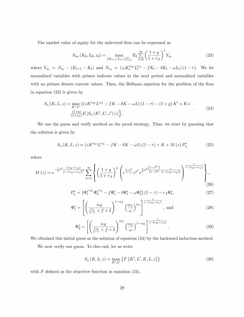
The market value of equity for the unlevered firm can be expressed as
Su0 (K0, L0, z0) = max{Kt+1,Lt+1}∞t=0
E0
∞∑t=0
(1 + g
1 + rA
)tYut (23)
where Yut = Nut − (Kt+1 −Kt) and Nut = (ztKαKt LαLt − fKt − δKt − ωLt) (1− τ). We let
normalized variables with primes indicate values in the next period and normalized variables
with no primes denote current values. Then, the Bellman equation for the problem of the firm
in equation (23) is given by
Su (K,L, z) = maxK′,L′
{(zKαKLαL − fK − δK − ωL) (1− τ)− (1 + g)K ′ +K+
(1+g)(1+rA)E [Su (K ′, L′, z′) |z]
}.
. (24)
We use the guess and verify method as the proof strategy. Thus, we start by guessing that
the solution is given by
Su (K,L, z) = (zKαKLαL − fK − δK − ωL) (1− τ) +K +M (z)P ∗u (25)
where
M (z) = e− 1
2σ2 (αK+αL)
[1−(αK+αL)]2∞∑n=1
(
1 + g
1 + rA
)nc 1−ρn1−ρ zρ
ne
12σ2 (1−ρ2n)
(1−ρ2)1
[1−(αK+αL)]
11−(αK+αL)
,
(26)
P ∗u =(Φ∗
αK
1 Φ∗αL
2 − fΦ∗1 − δΦ∗1 − ωΦ∗2)
(1− τ)− rAΦ∗1, (27)
Φ∗1 =
( αKrA
1−τ + f + δ
)1−αL (αLω
)αL 11−(αK+αL)
, and (28)
Φ∗2 =
[(αK
rA1−τ + f + δ
)αK (αLω
)1−αK] 1
1−(αK+αL)
. (29)
We obtained this initial guess as the solution of equation (24) by the backward induction method.
We now verify our guess. To this end, let us write
Su (K,L, z) = maxK′,L′
{F(K ′, L′,K, L, z
)}(30)
with F defined as the objective function in equation (24).
29

The FOC for this problem is
∂F (K ′, L′,K, L, z) /∂K ′ = − (1 + g) + (1+g)(1+rA)
[(E [z′|z]αKK∗αK−1L∗αL − f − δ
)(1− τ) + 1
]= 0
∂F (K ′, L′,K, L, z) /∂L′ = (1+g)(1+rA)
(E [z′|z]K∗αKαLL∗αL−1 − ω
)(1− τ) = 0
(31)
and optimal capital and labor turn out to be
K∗ = E[z′|z] 1
1−(αK+αL) Φ∗1 and L∗ = E[z′|z] 1
1−(αK+αL) Φ∗2 (32)
where Φ∗1 and Φ∗2 are as in equations (28) and (29), respectively.
Finally, the market value of equity for the unlevered firm becomes
Su (K,L, z) = (zKαKLαL − fK − δK − ωL) (1− τ)− (1 + g)K∗ +K+
(1+g)(1+rA) [(E [z′|z]K∗αKL∗αL − fK∗ − δK∗ − ωL∗) (1− τ) +K∗+
E [M (z′) |z]P ∗u ]
= (zKαKLαL − fK − δK − ωL) (1− τ) +K − (1 + g)E [z′|z]1
1−(αK+αL) Φ∗1+
(1+g)(1+rA)
{E [z′|z]
11−(αK+αL)
[(Φ∗
αK
1 Φ∗αL
2 − fΦ∗1 − δΦ∗1 − ωΦ∗2)
(1− τ) + Φ∗1]
+
E [M (z′) |z]P ∗u}
= (zKαKLαL − fK − δK − ωL) (1− τ) +K+
(1+g)(1+rA)
(e− 1
2σ2 (αK+αL)
[1−(αK+αL)]2E
[z′ 11−(αK+αL)K |z
]+ E [M (z′) |z]
)P ∗u
= (zKαKLαL − fK − δK − ωL) (1− τ) +K +M (z)P ∗u
(33)
which is equivalent to our initial guess in equation (25).
Next, we obtain optimal risky debt. In each period, the firm solves the following problem
maxB′,x′c
{B′ − 1
(1 + rB)
{B′ [1 + rB (1− τ)]− λ
(x′c)ξK
′}}
. (34)
where x′c is the cutoff value of the standard normal random variable x such that the probability
of x′ < x′c is λ (x′c).
The above problem can be solved in 2 steps. In the first step, given the value of x′c (i.e., for an
arbitrary probability of bankruptcy λ (x′c)), the firm chooses optimal debt B∗. Defining F as the
objective function in equation (34), the FOC turns out to be ∂F (K ′, B′, x′c) /∂B′ = 1
(1+rB)rBτ >
30
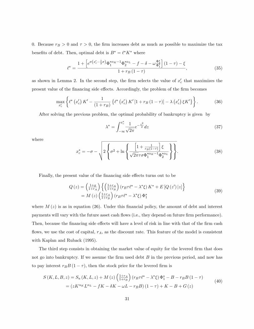
0. Because rB > 0 and τ > 0, the firm increases debt as much as possible to maximize the tax
benefits of debt. Then, optimal debt is B∗ = `∗K∗ where
`∗ =1 +
[eσ(x
′c− 1
2σ)Φ∗αK−1
1 Φ∗αL2 − f − δ − ωΦ∗2Φ∗1
](1− τ)− ξ
1 + rB (1− τ), (35)
as shown in Lemma 2. In the second step, the firm selects the value of x′c that maximizes the
present value of the financing side effects. Accordingly, the problem of the firm becomes
maxx′c
{`∗(x′c)K ′ − 1
(1 + rB)
{`∗(x′c)K ′ [1 + rB (1− τ)]− λ
(x′c)ξK ′
}}. (36)
After solving the previous problem, the optimal probability of bankruptcy is given by
λ∗ =
∫ x∗c
−∞
1√2πe−
z2
2 dz (37)
where
x∗c = −σ −
√√√√√2
σ2 + ln
[1 + 1
rB(1−τ)
]ξ
√2πτσΦ∗αK−1
1 Φ∗αL2
. (38)
Finally, the present value of the financing side effects turns out to be
Q (z) =(
1+g1+rA
){(1+rA1+rB
)(rBτ`
∗ − λ∗ξ)K∗ + E [Q (z′) |z]}
= M (z)(
1+rA1+rB
)(rBτ`
∗ − λ∗ξ) Φ∗1
(39)
where M (z) is as in equation (26). Under this financial policy, the amount of debt and interest
payments will vary with the future asset cash flows (i.e., they depend on future firm performance).
Then, because the financing side effects will have a level of risk in line with that of the firm cash
flows, we use the cost of capital, rA, as the discount rate. This feature of the model is consistent
with Kaplan and Ruback (1995).
The third step consists in obtaining the market value of equity for the levered firm that does
not go into bankruptcy. If we assume the firm used debt B in the previous period, and now has
to pay interest rBB (1− τ), then the stock price for the levered firm is
S (K,L,B, z) = Su (K,L, z) +M (z)(
1+rA1+rB
)(rBτ`
∗ − λ∗ξ) Φ∗1 −B − rBB (1− τ)
= (zKαKLαL − fK − δK − ωL− rBB) (1− τ) +K −B +G (z)(40)
31

where G (z) = M (z)P ∗ and variable P ∗ takes the form
P ∗ =(Φ∗
αK
1 Φ∗αL
2 − fΦ∗1 − δΦ∗1 − ωΦ∗2)
(1− τ)− rAΦ∗1 +
(1 + rA1 + rB
)(rBτ`
∗ − λ∗ξ) Φ∗1. (41)
Finally, the optimal decisions of the firm are given by
K∗ (zt) = (1 + g)E [zt+1|zt]1
1−(αK+αL) Φ∗1,
L∗ (zt) = (1 + g)E [zt+1|zt]1
1−(αK+αL) Φ∗2, and
B∗ (zt) = `∗K∗ (zt)
(42)
and the market value of equity is
S (Kt, Lt, Bt, zt) =[(1 + g)t[1−(αK+αL)] ztK
αKt LαLt − fKt − δKt − ωLt − rBBt
](1− τ) +
Kt −Bt +G (zt)
(43)
as shown in Proposition 1. �
32

Figure 1. Evolution of the market-to-value ratio. The figure displays the evolution over time
of the mean market-to-value ratio for a sample of firms included in the S&P 100 Index in the period
1990-2015. The market-to-value ratio is the market value of equity divided by the value estimated by the
model.
33

Figure 2. Cumulative strategy returns. The figure displays the cumulative returns of the port-
folio strategies for the P/V, P/B, and P/E portfolios during the 36 months following portfolio formation.
These portfolios are constructed with a sample of firms included in the S&P 100 Index in the period
1990-2015. P/V is the market-to-value ratio (i.e., the market value of equity divided by the equity value
estimated by the model). P/B is the market-to-book ratio (i.e., the market value of equity divided by
the book value of equity). P/E is the price-earnings ratio (i.e., the market value of equity divided by the
firm’s net income). Portfolios are formed by sorting firms into quintiles according to their P/V, P/B, and
P/E ratios at the end of May of each year. The portfolio strategy consists in buying firms in the bottom
quintile and selling firms in the top quintile.
34

Table 1
Cross-Sectional Parameter Values
The table presents the values used to parameterize the dynamic model of the firm for the different SIC
industries. The parameters are constant c, the persistence of profit shocks (ρ), the standard deviation of
the innovation term (σ), the concavity of the production function with respect to capital (αK) and labor
(αL), the operating costs (f), the capital depreciation rate (δ), labor wages (ω), the corporate income
tax rate (τ), the market cost of debt (rB), the market cost of capital (rA), the growth rate (g), and the
bankruptcy costs (ξ).
35

Table 2
Comparative Statics Analysis of Market Equity Value
The table exhibits the results of the sensitivity analysis of the stock price for different SIC industries.
The columns show the percentage variation in share price when the corresponding parameter changes by
1%. The parameters are constant c, the persistence of profit shocks (ρ), the standard deviation of the
innovation term (σ), the concavity of the production function with respect to capital (αK) and labor
(αL), the operating costs (f), the capital depreciation rate (δ), labor wages (ω), the corporate income
tax rate (τ), the market cost of debt (rB), the market cost of capital (rA), the growth rate (g), and the
bankruptcy costs (ξ).
36

Table 3
Valuation Results
The table shows the valuation results of the dynamic DDM for a sample of firms included in the S&P 100
Index in the period 1990-2015. P/V is the market-to-value ratio (i.e., the market value of equity divided
by the equity value estimated by the model). The log(P/V ) results derive from computing the log of the
market-to-value ratio. The first line in Panel B shows the percentage of times that the value estimated by
the model is within 15% of the market value of equity. The second line in Panel B shows the median value
of the absolute difference between the equity value estimated by the model and the market value of equity
(in percent). The third line in Panel B shows the median value of the squared difference between the value
estimated by the model and the market value of equity (in percent). Standard errors are in parentheses.
37

Table 4
Regression of the Market Value of Equity
The table shows the results from different cross-sectional regressions of the market value of equity. In
column (1), the regressor is the equity value estimated by the model; in column (2), the regressor is the
book value of equity; and in column (3), the regressor is net income. The sample is composed of firms
included in the S&P 100 Index in the period 1990-2015. Standard errors are in parentheses.
38

Table 5
Cumulative Portfolio Returns
The table presents the cumulative portfolio returns of three different strategies. P/V Portfolios is the
strategy that constructs portfolios based on the ranking of the market-to-value ratio (P/V ); P/B Portfolios
is the strategy that builds portfolios based on the ranking of the market-to-book ratio (P/B); and P/E
Portfolios is the strategy that constructs portfolios based on the ranking of the price-earnings ratio (P/E ).
Ret12, Ret24, and Ret36 are the average 12-month, 24-month, and 36-month portfolio returns of each
strategy, respectively. Q1-Q5 is the average spread of returns between the lowest (Q1 ) and highest (Q5 )
quintile portfolios. Ret/Risk is the ratio of the portfolio return to its standard deviation of returns. %
Winners is the percentage of periods (out of 20 years) in which the strategy yielded positive returns.
39

Table 6
Risk Exposure of the Portfolios
The table shows the results from regressions of the quintile portfolios’excess returns on the 3 Fama/French
risk factors. The regressor is the excess return of the P/V Portfolios, which is the strategy that constructs
portfolios based on the ranking of the market-to-value ratio (P/V ). Rm-Rf is the excess return on the
market, SMB (Small Minus Big) is the return on a portfolio of small stocks minus the return on a portfolio
of big stocks, and HML (High Minus Low) is the return on a portfolio of value stocks minus the return on
a portfolio of growth stocks. The sample is composed of the portfolio returns during the period 1990-2015.
Standard errors are in parentheses.
40