A Dynamic Model of Aggregate Demand and Aggregate Supply Chapter 15 of Macroeconomics, 8 th edition, by N. Gregory MankiwMacroeconomics ECO62ECO62 Udayan

A Dynamic Model of Aggregate Demand and Aggregate Supply

Chapter 15 of Macroeconomics, 8th edition, by N. Gregory Mankiw

ECO62 Udayan Roy

PART V Topics in Macroeconomic Theory

http://bcs.worthpublishers.com/mankiw7/

http://myweb.liu.edu/~uroy/eco62/index.html

http://myweb.liu.edu/~uroy/index.html



Inflation and dynamics in the short run

• So far, to analyze the short run we have used– the Keynesian Cross theory, and– the IS-LM theory

• Both theories are silent about – Inflation, and – Dynamics

• This chapter presents a dynamic short-run theory of output, inflation, and interest rates.

• This is the model of dynamic aggregate demand and dynamic aggregate supply (DAD-DAS)

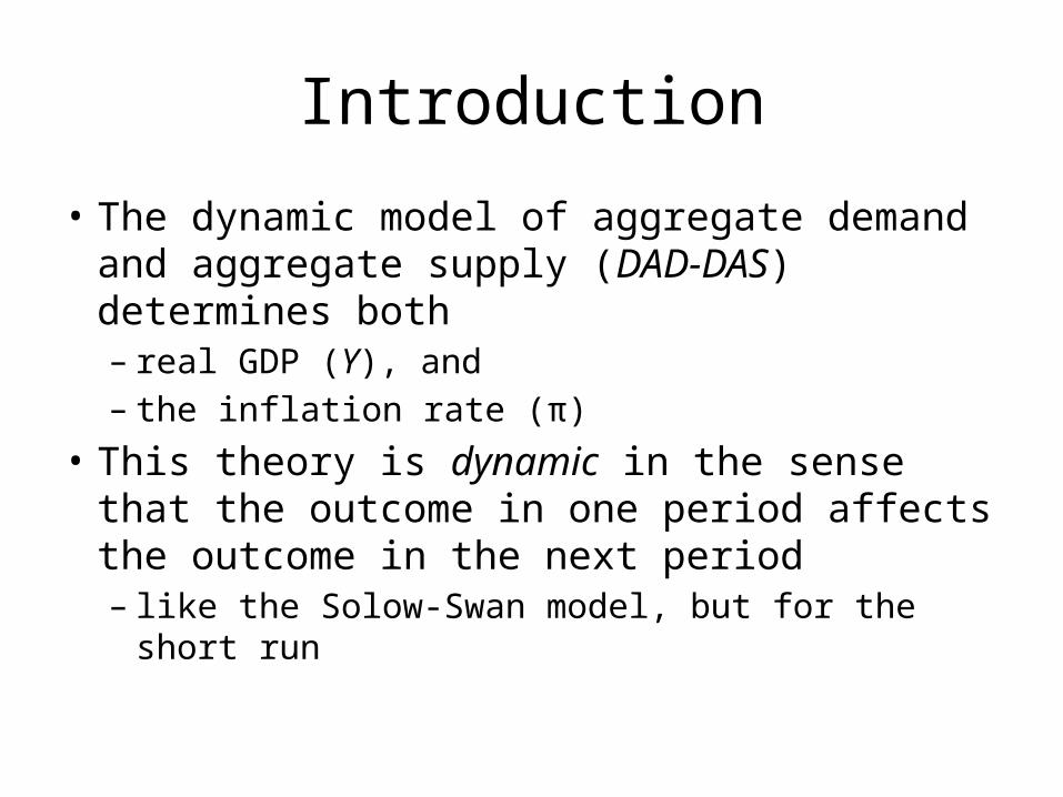
Introduction

• The dynamic model of aggregate demand and aggregate supply (DAD-DAS) determines both – real GDP (Y), and – the inflation rate (π)

• This theory is dynamic in the sense that the outcome in one period affects the outcome in the next period– like the Solow-Swan model, but for the short run

• Instead of representing monetary policy by an exogenous money supply, the central bank will now be seen as following a monetary policy rule – The central bank’s monetary policy rule adjusts

interest rates automatically when output or inflation are not where they should be.

Introduction

Introduction

• The DAD-DAS model is built on the following concepts:– the IS curve, which negatively relates the real interest

rate (r) and demand for goods and services (Y),– the Phillips curve, which relates inflation (π) to the gap

between output and its natural level (), expected inflation (Eπ), and supply shocks (ν),

– adaptive expectations, which is a simple model of expected inflation,

– the Fisher effect, and– the monetary policy rule of the central bank.

Keeping track of time

• The subscript “t ” denotes a time period, e.g.– Yt = real GDP in period t

– Yt − 1 = real GDP in period t – 1

– Yt + 1 = real GDP in period t + 1

• We can think of time periods as years. E.g., if t = 2008, then – Yt = Y2008 = real GDP in 2008

– Yt − 1 = Y2007 = real GDP in 2007

– Yt + 1 = Y2009 = real GDP in 2009

The model’s elements

• The model has five equations and five endogenous variables: – output, inflation, the real interest rate, the

nominal interest rate, and expected inflation. • The first equation is for output…

DAD-DAS: 5 Equations

• Demand Equation• Fisher Equation• Phillips Curve• Adaptive Expectations• Monetary Policy Rule

The Demand Equation

tttt rYY )(

Real GDP

Natural (or long-run or potential) Real GDP

Parameter representing the

response of demand to the real

interest rates

Real interest

rate

Natural (or long-run)

Real interest rate

Demand shock, represents

changes in G, T, C0, and I0

The Demand Equation

tttt rYY )(

α > 0

Assumption: ρ > 0; although the real interest rate can be negative, in the long run people will not lend their

resources to others without a positive return. This is the long-run real interest rate we had calculated in Ch. 3

Positive when C0, I0, or G is higher than usual or T is lower than usual.

Assumption: There is a negative relation between output (Yt) and interest rate (rt). The justification is the same as for the IS curve of Ch. 11

IS Curve = Demand Equation

• This graph is from Ch. 11

• Assume the IS curve is a straight line

• Then, for any pair of points—A and B, or C and B—the slope must be the same

𝒀Yt

r

Y

rt

𝒓IS

𝒀Yt

r

Y

rt

𝒓IS

A

B

BC


• Then, for any point (rt, Yt) on the line, we get , a constant.

𝒀Yt

r

Y

rt

𝒓IS

𝒀Yt

r

Y

rt

𝒓IS The long-run real equilibrium interest rate of

Figure 3-8 in Ch. 3 is now denoted by the lower-case Greek letter ρ.


• Now, we also saw in Ch. 12 that the IS curve can shift when there are changes in C0, I0, G, and T

• To represent all these shift factors, we add the random demand shock, εt.

• Therefore, the IS curve of Ch. 12 gives us this chapter’s demand equation


• The IS curve can simply be renamed the Demand Equation curve

𝒀

rt

Yt

ρDemand

𝒀 𝐭

rt

Yt

ρIS

tttt rYY )(

Demand Equation Curve

𝒀 +𝜺𝒕

rt

Yt

ρDemand

tttt rYY )(

Note that if increases (decreases) by some amount, the Demand equation curve shifts right (left) by the same amount.

Note also that if ρ increases (decreases) by some amount, the Demand equation curve shifts up (down) by the same amount.



The Real Interest Rate: The Fisher Equation

1t t t tr i E

nominal interest

rate

expected inflation rate

ex ante (i.e. expected)

real interest rate

Assumption: The real interest rate is the inflation-adjusted interest rate. To adjust the nominal interest rate for inflation, one must simply subtract the expected inflation rate during the duration of the loan.

The Real Interest Rate: The Fisher Equation

1t t t tr i E

nominal interest

rate

expected inflation rate

ex ante (i.e. expected)

real interest rate

increase in price level from period t to t +1, not known in period t

expectation, formed in period t, of inflation from t to t +1

1t

1t tE

We saw this before in Ch. 5



Inflation: The Phillips Curve

1 ( )t t t t t tE Y Y

previously expected inflation

current inflation

supply shock,

random and zero on average indicates how much

inflation responds when output fluctuates around

its natural level

0

Phillips Curve

• Assumption: At any particular time, inflation would be high if– people in the past were expecting it to be high– current demand is high (relative to natural GDP)– there is a high inflation shock. That is, if prices are

rising rapidly for some exogenous reason such as scarcity of imported oil or drought-caused scarcity of food

tttttt YYE 1

Phillips Curve

tttttt YYE 1

• This Phillips Curve can be seen as summarizing three reasons for inflation

Momentum inflation

Demand-pull

inflation

Cost-push inflation



Expected Inflation: Adaptive Expectations

1t t tE

Assumption: people expect prices to continue rising at the current inflation rate.

Examples: E2000π2001 = π2000; E2013π2014 = π2013; etc.



Monetary Policy Rule

• The fifth and final main assumption of the DAD-DAS theory is that– The central bank sets the nominal interest rate – and, in setting the nominal interest rate, the

central bank is guided by a very specific formula called the monetary policy rule


ttYtttt YYi *

Nominal interest rate, set each period by the central bank

Current inflation rate

Natural real interest rate

Parameter that measures how strongly the central bank responds to the inflation gap

Parameter that measures how strongly the central bank responds to the GDP gap

Inflation Gap: The excess of current inflation over the central bank’s inflation target

GDP Gap: The excess of current GDP over natural GDP

Example: The Taylor Rule• Economist John Taylor proposed a monetary policy rule

very similar to ours:

iff = + 2 + 0.5 ( – 2) – 0.5 (GDP gap)

where

– iff = nominal federal funds rate target

– GDP gap = 100 x

= percent by which real GDP is below its natural rate

• The Taylor Rule matches Fed policy fairly well.…

Y Y

Y

CASE STUDYThe Taylor Rule

1987 1989 1991 1993 1995 1997 1999 2001 2003 2005 2007 20090

1

2

3

4

5

6

7

8

9

10

Percent

Taylor’s rule

actual Federal

Funds rate

SUMMARY OF THE DAD-DAS MODEL

The model’s variables and parameters

• Endogenous variables:

tY

tr

t

1t tE ti

Output

Inflation

Real interest rate

Nominal interest rate

Expected inflation


• Exogenous variables:

• Predetermined variable:

tY *t

t

t

1t

Natural level of output

Central bank’s target inflation rate

Demand shock

Supply shock

Previous period’s inflation


• Parameters:

Y

Responsiveness of demand to the real interest rate

Natural rate of interest

Responsiveness of inflation to output in the Phillips Curve

Responsiveness of i to inflation in the monetary-policy rule

Responsiveness of i to output in the monetary-policy rule

The DAD-DAS Equations

ttYtttt

ttt

tttttt

tttt

tttt

YYi

E

YYE

Eir

rYY

*

1

1

1

)( Demand Equation

Fisher Equation

Phillips Curve

Adaptive Expectations


DYNAMIC AGGREGATE SUPPLY

Recap: Dynamic Aggregate Supply

ttt

tttttt

E

YYE

1

1Phillips Curve

Adaptive Expectations

ttttt YY 1 DAS Curve

11 tttE

The Dynamic Aggregate Supply Curve

DAS slopes upward: high levels of output are associated with high inflation. This is because of demand-pull inflation

Yt

πt

DASt

tY

tt 1

ttttt YY 1


Y

π

DAS2011

1 ( ) t t t t tY Y

2011Y

20112010

If you know (a) the natural GDP at

a particular date, (b) the inflation shock

at that date, and (c) the previous

period’s inflation,you can figure out the location of the DAS curve at that date.


Y

π

DAS2015

1 ( ) t t t t tY Y

2015Y

20152014

If you know (a) the natural GDP at

a particular date, (b) the inflation shock

at that date, and (c) the previous

period’s inflation,you can figure out the location of the DAS curve at that date.

Shifts of the DAS Curve

Y

π

DASt

1 ( ) t t t t tY Y

tY

tt 1

Any increase (decrease) in the previous period’s inflation or in the current period’s inflation shock shifts the DAS curve up (down) by the same amount

Shifts of the DAS Curve

Y

π

DASt

1 ( ) t t t t tY Y

tY

tt 1

Any increase (decrease) in the previous period’s inflation or in the current period’s inflation shock shifts the DAS curve up (down) by the same amount

Any increase (decrease) in natural GDP shifts the DAS curve right (left) by the exact amount of the change.

DYNAMIC AGGREGATE DEMANDBuckle up for some tedious algebra!

The Dynamic Aggregate Demand Curve

( )t t t tY Y r

1( ) t t t t t tY Y i E

Fisher equation1 tttt Eir

( ) t t t t tY Y i adaptive

expectations

tttE 1

The Demand Equation


( ) t t t t tY Y i

*[ ( ) ( ) ] t t t t t Y t t t tY Y Y Y

monetary policy rule

*[ ( ) ( )] t t t t Y t t tY Y Y Y

ttYtttt YYi *

We’re almost there!

Dynamic Aggregate Demand*[ ( ) ( )] t t t t Y t t tY Y Y Y

ttttt

tY

ttY

tt

ttttYtY

ttYttttYt

ttYtYtttt

BAYY

YY

YY

YYYY

YYYY

)(

1

1)(

1

)()1()1(

)(

)(

*

*

*

*

*

This is the equation of the DAD curve!


DAD slopes downward:When inflation rises, the central bank raises the real interest rate, reducing the demand for goods and services.

Y

π

DADt

Note that the DAD equation has no dynamics in it: it only shows how simultaneously measured variables are related to each other

𝑌 𝑡=𝑌 𝑡−𝐴 ∙ (𝜋𝑡− 𝜋∗𝑡 )+𝐵 ∙𝜀𝑡


Y

π

DADtB

*t

tt BY



Y

π

DADt1

*t

tt BY

When the central bank’s target inflation rate increases (decreases) the DAD curve moves up (down) by the exact same amount.

DADt2


Note how monetary policy is described in terms of the target inflation rate in the DAD-DAS model

Monetary Policy

• In the IS-LM model, monetary policy was described by the money supply or the interest rate– Expansionary monetary policy meant M↑ or i↓– Contractionary monetary policy meant M↓ or i↑

• In the DAD-DAS model, – Expansionary monetary policy is π*↑– Contractionary monetary policy is π*↓


Y

π

DADt1

*t

tt BY

When the natural rate of output increases (decreases) the DAD curve moves right (left) by the exact same amount.

When there is a positive (negative) demand shock the DAD curve moves right (left) .

A positive demand shock could be an increase in C0, I0, or G, or a decrease in T.

DADt2



Y

π

The DAD curve shifts right or up if:1. the central bank’s target

inflation rate goes up, 2. there is a positive demand

shock, or 3. the natural rate of output

increases.DADt1

DADt2


SUMMARY: DAS AND DAD EQUATIONS

Summary: DAS and DAD Equations

• Note that there are two endogenous variables—Yt and πt

—in these two equations• Therefore, we can solve for the equilibrium values of Yt

and πt

tY

ttY

tt YY

1

1)(

1*

ttttt YY 1DAS

DAD

The Solution!

Using the equations in the previous slide—and a lot of very tedious algebra—one can express output and inflation entirely in terms of exogenous variables, parameters, shocks and pre-determined inflation. This is the algebraic solution of the DAD-DAS model.

The Solution!

• And once we solve for the equilibrium values of Yt and πt,

• we can use adaptive expectations to solve for expected inflation: .

• We can use the monetary policy rule to determine the nominal interest rate

• and the Fisher Effect to solve for the real interest rate

The Solution!

By substituting the previous slide’s solutions for output and inflation into the monetary policy rule, we can then get the above solution for the nominal interest rate. The Fisher equation can be used to solve for the real interest rate.

Please do not worry about the solution and its derivation. However, if you are interested, please see http://myweb.liu.edu/~uroy/eco62/ppt/zlb-educ130328.pdf.pdf, especially sections 4.1 , 8.1 (appendix) and 8.2 (appendix).

http://myweb.liu.edu/~uroy/eco62/ppt/zlb-educ130328.pdf.pdf

Summary: DAD-DAS Slopes and Shifts

DAS• Upward sloping• If natural output increases,

shifts right by same amount• If previous-period inflation

increases, shifts up by same amount

• If there is a positive inflation shock (νt > 0), shifts up by same amount

DAD• Downward sloping• If natural output increases,

shifts right by same amount• If target inflation increases,

shifts up by same amount• If there is a positive demand

shock (εt > 0), shifts right

DAD-DAS LONG-RUN EQUILIBRIUM

The DAD-DAS model’s long-run equilibrium

• This is the normal state around which the economy fluctuates.

• Definition: The economy is in long-run equilibrium when:– There are no shocks:

– Inflation is stable:

Long-Run Equilibrium

• DAS: • In long-run equilibrium all shocks are zero.• Therefore, • In long-run equilibrium inflation is stable (). • Therefore, in long-run equilibrium, GDP is .


• We just saw that, in long-run equilibrium, GDP is .• Therefore, in long-run equilibrium, inflation is .• Moreover, by the Fisher effect, expected inflation is:

.

)(1

1

1)(

1

*

*

ttY

tt

tY

ttY

tt

YY

YY

In long-run equilibrium all shocks are zero

DAD


• The monetary policy rule is: • As and , we see that

– the long-run nominal interest rate is , – and the long-run real interest rate is

• Solved!

The DAD-DAS model’s long-run equilibrium

• To summarize, the long-run equilibrium values in the DAD-DAS theory are essentially the same as the long run theory we saw earlier in this course:

t tY Y

tr *

t t *

1t t tE *

t ti

In the short-run, the values of the various variables fluctuate around the long-run equilibrium values.

DAD-DAS SHORT-RUN EQUILIBRIUM

Yt

The short-run equilibrium

In each period, the intersection of DAD and DAS determines the short-run equilibrium values of inflation and output.

πt

Yt

Y

π

DADt

DASt

AIn the equilibrium shown here at A, output is below its natural level. In other words, the DAD-DAS theory is fully capable of explaining recessions and booms.

DAD-DAS PREDICTIONS

How does the economy respond—in the short run and in the long run—to (i) an increase in potential output, (ii) a temporary inflation shock, (iii) a temporary demand shock, and (iv) stricter monetary policy?

Long-Run Growth

• Suppose an economy is in long-run equilibrium

• We saw in Chapters 8 and 9 that an economy’s natural GDP can increase over time

• If , what will be the short-run effect on our five endogenous variables?

• In what way will the economy adjust from the old long-run equilibrium to the new long-run equilibrium?

Recap: DAD-DAS Slopes and Shifts


shifts right by same amount

• If previous-period inflation increases, shifts up by same amount



shifts right by same amount

• If target inflation increases, shifts up by same amount

• If there is a positive demand shock (εt > 0), shifts right

Long-run growthPeriod t: initial equilibrium at A

Y

π

DASt

Yt

DADt

A

Yt

Period t + 1: Long-run growth increases the natural rate of output.

Yt +1

DASt +1

DADt +1

Bπt + 1

πt

=

DAS shift right by the exact amount of the increase in natural GDP.

DAD shifts right too by the exact amount of the increase in natural GDP.New equilibrium at B. Income grows but inflation remains stable.

Yt +1

Long-Run Growth

• Therefore, starting from long-run equilibrium, if there is an increase in the natural GDP,– actual GDP will immediately increase to the new

natural GDP, and– none of the other endogenous variables will be

affected

Inflation Shock

• Suppose the economy is in long-run equilibrium

• Then the inflation shock hits for one period (νt > 0) and then goes away (νt+1 = 0)

• How will the economy be affected, both in the short run and in the long run?










A shock to aggregate supply

Period t – 1: initial equilibrium at A

πt – 1

Yt –1

Period t: Supply shock (νt > 0) shifts DAS upward; inflation rises, central bank responds by raising real interest rate, output falls.

Period t + 1: Supply shock is over (νt+1 = 0) but DAS does not return to its initial position due to higher inflation expectations.

Period t + 2: As inflation falls, inflation expectations fall, DAS moves downward, output rises.

Y

π

DASt -1

Y

DAD

A

DASt

Yt

Bπt

DASt +1

C

DASt +2

D

Yt + 2

πt + 2

This process continues until output returns to its natural rate. The long run equilibrium is at A.

A shock to aggregate supply: one more time

π2000 = π2001

Y01

Y

π

DAS2001

Y

DAD

A

DAS2002

Y02

Bπ2002

DAS2003

CD

DAS2004

Y03

π2003

π2001 + ν2002

π2004

Y04

ν2002

Inflation Shock

• So, we see that if a one-period inflation shock hits the economy,– inflation rises at the date the shock hits, but

eventually returns to the unchanged long-run level, and

– GDP falls at the date the shock hits, but eventually returns to the unchanged long-run level

• What happens to the interest rates i and r?

Inflation Shock

• According to the monetary policy rule, the temporary spike in inflation dictates an increase in the real interest rate, whereas the temporary fall in GDP indicates a decrease in the real interest rate

• The overall effect is ambiguous, for both interest rates• We can do simulations for specific values of the parameters

and exogenous variables

ttYttt

ttYtttt

ttYtttt

YYr

YYi

YYi

*

*

*

Recall: The Solution!

As we saw before, it is possible to express output and inflation entirely in terms of exogenous variables, parameters, shocks and pre-determined inflation. The monetary policy rule can then be used to solve for the nominal interest rate. The Fisher equation can be used to solve for the real interest rate. These solutions can be used to simulate the future outcomes for given values of the exogenous terms in the equations.

Thus, we can interpret as the percentage deviation of output from its natural level.

Parameter values for simulations100tY

* 2.0t1.0

2.00.25

0.50.5Y

The central bank’s inflation target is 2 percent.

A 1-percentage-point increase in the real interest rate reduces output demand by 1 percent of its natural level.

The natural rate of interest is 2 percent.

When output is 1 percent above its natural level, inflation rises by 0.25 percentage point.

These values are from the Taylor Rule, which approximates the actual behavior of the Federal Reserve.

Impulse Response Functions

• The following graphs are called impulse response functions.

• They show the “response” of the endogenous variables to the “impulse,” i.e. the shock.

• The graphs are calculated using our assumed values for the exogenous variables and parameters

The dynamic response to a supply shock

tY

t

A one-period supply shock affects output for many periods.


t

t Because inflation expectations adjust slowly, actual inflation remains high for many periods.


tr

t

The real interest rate takes many periods to return to its natural rate.


ti

tThe behavior of the nominal interest rate depends on that of inflation and real interest rates.

A Series of Aggregate Demand Shocks

• Suppose the economy is at the long-run equilibrium

• Then a positive aggregated demand shock hits the economy for five successive periods (εt, εt+1, εt+2, εt+3, εt+4 > 0), and then goes away (εt+5 = 0)

• How will the economy be affected in the short run?

• That is, how will the economy adjust over time?








shifts up by same amount• If there is a positive

demand shock (εt > 0), shifts right

A shock to aggregate demandPeriod t – 1: initial equilibrium at A

πt – 1

Y

π

DASt -1,t

Y

DADt ,t+1,…,t+4

DADt -1, t+5

DASt +5

Yt –1

A

DASt + 1

C

DASt +2

D

DASt +3

E

DASt +4

F

Yt

Bπt

Yt + 5

Gπt + 5

Period t: Positive demand shock (ε > 0) shifts AD to the right; output and inflation rise.

Period t + 1: Higher inflation in t raised inflation expectations for t + 1, shifting DAS up. Inflation rises more, output falls.

Periods t + 2 to t + 4:Higher inflation in previous period raises inflation expectations, shifts DAS up. Inflation rises, output falls.Period t + 5: DAS is higher due to higher inflation in preceding period, but demand shock ends and DAD returns to its initial position. Equilibrium at G.

Periods t + 6 and higher:DAS gradually shifts down as inflation and inflation expectations fall. The economy gradually recovers and reaches the long run equilibrium at A.

A 3-period shock to aggregate demand

π1999 = π00

Y

π

DAS00,01

Y

DAD01,02,03

DAD00,04

Y00

A

DAS02

C

Y01

Bπ01

DAS03

Dπ02

π03

Y02Y03

DAS04

When the demand shock first hits, output and inflation both increase. In the two following periods, despite the continuing presence of the demand shock, output starts to fall. Inflation continues to rise.

A shock to aggregate demand

π1999 = π00

Y

π

DAS00,01

Y

DAD00,04,05,06

Y00

A

π03

Y05Y04

DAS04

π04

DAS05DAS06

π05

On the date the demand shock ends, output falls below the long-run level and inflation finally begins to fall. After that, output rises and inflation falls towards the initial long-run equilibrium.

EF

A 3-period shock to aggregate demand

π1999 = π00

Y

π Y

Y00

A

C

Y01

Bπ01

Dπ02

π03

Y02Y03

In short, after a positive demand shock we get a counter-clockwise cycle in the output-inflation graph. But this is also a clockwise cycle in the unemployment-inflation graph.

Y05Y04

π04π05

FE

π

unemployment

Clockwise cycle

Counter-clockwise cycle

Inflation-Unemployment Cycles

• Please see:– http://krugman.blogs.nytimes.com/2010/07/31/cl

ockwise-spirals/– http://krugman.blogs.nytimes.com/2011/11/17/s

ubsiding-inflation/– http://

krugman.blogs.nytimes.com/2012/04/08/unemployment-and-inflation/

http://krugman.blogs.nytimes.com/2012/04/08/unemployment-and-inflation/








A Series of Aggregate Demand Shocks: 4 Phases

1. On the date the multi-period demand shock first hits, both output and inflation rise above their long-run values

2. After that, while the demand shock is still present, output falls and inflation continues to rise

3. On the date the demand shock ends, output falls below its long-run value and inflation falls

4. After that, output recovers and inflation falls, gradually returning to their original long-run values

• What happens to the interest rates i and r?

A Series of Aggregate Demand Shocks: 4 Phases, interest rates

1. On the date the multi-period demand shock first hits, both output and inflation rise above their long-run values. So, interest rate rises

2. After that, while the demand shock is still present, output falls and inflation continues to rise. Now, the effect on the interest rate is ambiguous

3. On the date the demand shock ends, output falls below its long-run value and inflation falls. So, the interest rate falls

4. After that, output recovers and inflation falls, gradually returning to their original long-run values. Again, the effect on the interest rate is ambiguous, but it does return to its original long run value (ρ)

The dynamic response to a demand shock

tY

t

The demand shock raises output for five periods. When the shock ends, output falls below its natural level, and recovers gradually.


t

tThe demand shock causes inflation to rise. When the shock ends, inflation gradually falls toward its initial level.


tr

t

The demand shock raises the real interest rate. After the shock ends, the real interest rate falls and approaches its initial level.


ti

tThe behavior of the nominal interest rate depends on that of the inflation and real interest rates.

Stricter Monetary Policy

• Suppose an economy is initially at its long-run equilibrium

• Then its central bank becomes less tolerant of inflation and reduces its target inflation rate (π*) from 2% to 1%

• What will be the short-run effect?• How will the economy adjust to its new long-

run equilibrium?










A shift in monetary policyPeriod t – 1: target inflation rate π* = 2%, initial equilibrium at A

πt – 1 = 2%

Yt –1

Period t: Central bank lowers target to π* = 1%, raises real interest rate, shifts DAD leftward. Output and inflation fall.Period t + 1: The fall in πt reduced inflation expectations for t + 1, shifting DAS downward. Output rises, inflation falls.

Y

πDASt -1, t

Y

DADt – 1

A

DADt, t + 1,…

DASfina

l

Yt

πtB

DASt +1

C

Subsequent periods:This process continues until output returns to its natural rate and inflation reaches its new target.

Zπfinal = 1%

,

Yfinal

Stricter Monetary Policy

• At the date the target inflation is reduced, output falls below its natural level, and inflation falls too towards its new target level– The real interest rate rises above its natural level (ρ)– The effect on the nominal interest rate (i = r + π) is ambiguous

• On the following dates, output recovers and gradually returns to its natural level. Inflation continues to fall and gradually approaches the new target level.– The real interest rate falls, gradually returning to its natural level

(ρ)– The nominal interest rate falls to its new and lower long-run

level (i = ρ + π*)

The dynamic response to a reduction in target inflation

tY

*t

Reducing the target inflation rate causes output to fall below its natural level for a while. Output recovers gradually.


t

*t

Because expectations adjust slowly, it takes many periods for inflation to reach the new target.


tr

*t

To reduce inflation, the central bank raises the real interest rate to reduce aggregate demand.The real interest rate gradually returns to its natural rate.


ti

*t

The initial increase in the real interest rate raises the nominal interest rate. As the inflation and real interest rates fall, the nominal rate falls.

APPLICATION:Output variability vs. inflation variability

• A supply shock reduces output (bad) and raises inflation (also bad).

• The central bank faces a tradeoff between these “bads” – it can reduce the effect on output, but only by tolerating an increase in the effect on inflation….


CASE 1: θπ is large, θY is small

Y

π

DADt – 1, t

DASt

DASt – 1

Yt –1

πt –1

Yt

πt

A supply shock shifts DAS up. In this case, a small

change in inflation has a large effect on output, so DAD is relatively flat.

The shock has a large effect on output, but a small effect on inflation.


CASE 2: θπ is small, θY is large

Y

π

DADt – 1, t

DASt

DASt – 1

Yt –1

πt –1

Yt

πt

In this case, a large change in inflation has only a small effect on output, so DAD is relatively steep.

Now, the shock has only a small effect on output, but a big effect on inflation.

APPLICATION:The Taylor Principle

• The Taylor Principle (named after economist John Taylor): The proposition that a central bank should respond to an increase in inflation with an even greater increase in the nominal interest rate (so that the real interest rate rises). I.e., central bank should set θπ > 0.

• Otherwise, DAD will slope upward, economy may be unstable, and inflation may spiral out of control.


If θπ > 0:

• When inflation rises, the central bank increases the nominal interest rate even more, which increases the real interest rate and reduces the demand for goods and services.

• DAD has a negative slope.

* 1( )

1 1

t t t t tY Y

Y Y

(DAD)

*( ) ( ) t t t t Y t ti Y Y (MP rule)


If θπ < 0:

• When inflation rises, the central bank increases the nominal interest rate by a smaller amount. The real interest rate falls, which increases the demand for goods and services.

• DAD has a positive slope.

* 1( )

1 1

t t t t tY Y

Y Y

(DAD)

*( ) ( ) t t t t Y t ti Y Y (MP rule)


• If DAD is upward-sloping and steeper than DAS, then the economy is unstable: output will not return to its natural level, and inflation will spiral upward (for positive demand shocks) or downward (for negative ones).

• Estimates of θπ from published research:

– θπ = – 0.14 from 1960-78, before Paul Volcker became Fed chairman. Inflation was high during this time, especially during the 1970s.

– θπ = 0.72 during the Volcker and Greenspan years. Inflation was much lower during these years.

Documents

A Dynamic Model of Aggregate Demand and Aggregate Supply Chapter 15 of Macroeconomics, 8 th edition, by N. Gregory MankiwMacroeconomics ECO62ECO62 Udayan