Embed Size (px)
Citation preview
A Dynamic Analysis of Nash Equilibria in Search
Models with Fiat Money�
Federico Bonetto, School of Mathematics, Georgia Tech
Maurizio Iacopetta, OFCE (Sciences-Po) and Skema Business School
Abstract
We study the rise in the acceptability �at money in a Kiyotaki-Wright economy by
developing a method that can determine dynamic Nash equilibria for a class of search
models with genuine heterogenous agents. We also address open issues regarding the
stability properties of pure strategies equilibria and the presence of multiple equilibria.
Experiments illustrate the liquidity conditions that favor the transition from partial
to full acceptance of �at money, and the e¤ects of in�ationary shocks on production,
liquidity, and trade.
Keywords: Acceptability of Money, Perron, Search.JEL codes: C61, C62, D83, E41.
1 Introduction
One central question of monetary economics is how an object that does not bring utility per
se is accepted as a mean of payment. It is well understood that the emergence of money
depends on trust and coordination of believes. While some recognize this observation and
simply assume that money is part of the economic system, others have tried to explain the
acceptance of money as the result of individuals�interactions in trade and production activi-
ties.1 Among the best-known attempts to formalize the emergence of money in decentralized
�Correspondence to: [email protected]. We are grateful to conference and seminar partici-
pants at the 2017 Summer Workshop on Money, Banking, Payments, and Finance at the Bank of Canada, the
IV AMMCS International Conference, Waterloo, Canada, Luiss University (Rome), University of Göttingen,
and the School of Mathematics, Georgia Tech, for useful comments.1Economic textbooks sometimes alert readers that the acceptance of �at money cannot be taken for
granted. For instance, Mankiw (2006, p. 644-45) observes that in the late 1980s, when the Soviet Union was
breaking up, in Moscow some preferred cigarettes to rubles as means of payment.
1
exchanges is Kiyotaki and Wright (1989) (henceforth, KW). The static analysis in KW pro-
vides important insights on how specialization in production, the technology of matching,
and the cost of holding commodities, condition the emergence of monetary equilibria. Never-
theless, it leaves important issues open. First, one would like to know if and how convergence
to a particular long run equilibrium occurs from an arbitrary initial state of the economy.
Historical accounts describe di¤erent patterns that societies followed in adopting objects as
means of payment.2 What are the dynamic conditions that lead individuals in a KW econ-
omy to accept commodity or �at money? Second, static analysis gives little guidance about
the short run consequences of a shock that causes, for instance, a sudden rise of in�ation.
How does the degree of acceptability of commodity and �at money change with in�ation?
The determination of dynamic equilibria in a KW environment is challenging. In an e¤ort
to improve its tractability, new classes of monetary search models have been proposed. These
have incorporated some features of centralized exchanges but have also eliminated others,
most notably the genuine heterogeneity across individuals and goods, and the storability of
goods (see Lagos et al. (2017), for a recent review). Restoring these features turns out to
be a useful exercise for characterizing the rise of money as a dynamic phenomenon.
The study of money acceptance in a KW environment requires a departure from the con-
ventional set of tools employed to characterize the dynamics of an economy with centralized
markets. Our method combines Nash�s (1950) de�nition of equilibrium with Perron�s iter-
ative approach to prove the stable manifold theorem (see, among others, Robinson, 1995).
This is the �rst work, to our knowledge, that shows how to determine pure strategies dy-
namic Nash equilibria in a KW search environment with �at money. Previous works on the
subject considered economies without �at money, and often assumed bounded rationality.3
Steady state results echo those of inventory-theoretic models of money (e.g., Baumol
1952, Tobin 1956, and Jovanovic 1982): for instance, higher levels of seignorage may induce
some to keep commodities in the inventory instead of accepting money, as a way to minimize
the odds of being hit by a seignorage tax. The dynamic analysis, however, generates novel
results: it shows how changes in the liquidity of assets other than money can alter the
2For a classic review of the rise of early means of payments see Quiggin (1949). For the institutional and
historical conditions that favored the dissemination of �at money see Goetzmann (2016).3See, for instance, the works of Marimon et al. (1990) and Basç¬ (1999) with intelligent agents, and
of Brown (1996) and Du¤y and Ochs (1999, 2002) with controlled laboratory experiments. Matsuyama et
al. (1993), Wright (1995), Luo (1999) and Sethi (1999) use evolutionary dynamics. Kehoe, Kiyotaki, and
Wright (1993) show that under mixed strategies equilibria could generate cycles, sunspots, and other non-
Markovian equilibria. Renero (1998), however, proves that it is impossible to �nd an initial condition from
which an equilibrium pattern converges to a mixed strategy steady state equilibrium. Ober�eld and Trachter
(2012) �nd that, in a symmetric environment, as the frequency of search increases, cycles and multiplicity
in mixed strategy tend to disappear. More recently, Iacopetta (2018) studies dynamic Nash equilibria in a
KW environment with no �at money.
2
proportion of individuals who accept �at money in transactions. For instance, it reveals that
an economy that converges to a long run equilibrium in which all prefer �at money to all
types of commodities (full acceptance), may go through a phase in which only a fraction of
individuals do so (partial acceptance).4
The remainder of the paper is organized as follows. Section 2 describes the economic
environment, characterizes the evolution of the distribution of inventories and money, and
de�nes a Nash equilibrium. Section 3 overviews steady state Nash equilibria for some spec-
i�cations of the model. Section 4 presents a methodology to determine Nash equilibria.
Section 5 illustrates the acceptability of money and discusses multiple steady states through
numerical experiments. Section 6 contains welfare considerations. Section 7 has few remarks
about future research. Appendix A contains proofs and mathematical details omitted in the
main text. Appendix B explains how the stable manifold theorem is related to our solution
algorithm.
2 The Model
This section describes the economic environment, characterizes the evolution of the distrib-
ution of inventories and money, and de�nes a Nash equilibrium.
2.1 The Environment
The model economy is a generalization of that described in KW. There are four main dif-
ferences. First, to facilitate the analysis of the dynamics, time is continuous. Second, the
model is extended to deal with seignorage, following the approach devised by Li (1994,
1995): government agents randomly con�scate money holders of their balances and use the
proceedings to purchase commodities. Third, as in Wright (1995) agents are not necessarily
equally divided among the three types. Fourth, as in Lagos et al. (2017), we obtain the type
of equilibria that emerge in the Model B of KW by reshu ing the ordering of the storage
costs across the three types of goods rather than altering the patterns of specialization in
production.
The economy is populated by three types of in�nitely lived agents; there areNi individuals
of type i, with i = 1; 2; 3, where Ni is a very large number. The total size of the population
is N = N1 + N2 + N3 and the fraction of each type is denoted with �i = NiN. A type i
agent consumes only good i and can produce only good i+1 (modulo 3). Production occurs
immediately after consumption. Agent i�s instantaneous utility from consuming a unit of
4Shevchenko and Wright (2004) also study partial acceptability in pure strategies. They focus, however,
on steady state analysis.
3

good i and the disutility of producing good i + 1 are denoted by Ui and Di, respectively,
with Ui > Di > 0, and their di¤erence with ui = Ui �Di. The storage cost of good i is ci,
measured in units of utility.5 In addition to the three types of commodity there is a fourth
object, called money and denoted by m, that does not bring utility per se: it only serves
as a means of transaction. Fiat money is indivisible. Denoting with M the fraction of the
population holding �at money, the total quantity of �at money is Q = NM . There is no
cost for storing money. At each instant in time, an individual can hold one and only one
unit of any type i good or one unit of money.6
The discount rate is denoted by � > 0. A pair of agents is randomly and uniformly
chosen from the population to meet for a possible trade. The matching process is governed
by a Poisson process with exogenous arrival rate �N2, where � > 0 �i.e. there is a constant
returns to scale matching technology. Hence, after a pair is formed, the expected waiting
time for the next pair to be formed is 2�N. A bilateral trade occurs if, and only if, it is
mutually agreeable. Agent i always accepts good i but never holds it because, provided
that ui is su¢ ciently large, there is immediate consumption (see KW, Lemma 1, p. 933).
Therefore, agent i enters the market with either one unit of good i+1, or i+2, or with one
unit of m.
We introduce seignorage as Li (1994, 1995): The government extracts seignorage revenue
from money holders in the form of a money tax �this device has been used by many others,
including in the recent work of Deviatov and Wallace (2014). In particular, government
agents meet and con�scate money from money holders. The arrival rate of a government
agent for a money holder is �m. A money holder of type i, whose unit of money is con�scated,
returns to the state of production without consumption, produces a new commodity i + 1,
and incurs a disutilityDi. With the proceedings of the tax revenue the government purchases
goods from commodity holders. These encounters are governed by a Poisson process with
arrival rate �g. The government runs, on average, a balanced budget. This requires that
�mM = �g(1 �M); implying that �g = �mM1�M . We allow the government to alter the rate
of seignorage �m, but, in order to simplify the dynamic analysis, the government does not
change the real balances in circulation �i.e. the initial level of �at money is given and does
not change over time. We will compare, however, steady state equilibria of economies with
di¤erent levels of M .5There is no restriction on the sign of ci. A negative storage cost is equivalent to a positive return.6The assumption that an individual can have either 0 or 1 unit of an asset greatly simpli�es the analysis
and makes more transparent the decision about the acceptance of money. There is a signi�cant amount of
work with asset-holding restrictions. See, among others, Diamond (1982), Rubinstein and Wolinsky (1987),
Cavalcanti and Wallace (1999), and Du¢ e et al. (2005).
4
2.2 Distribution of Commodities and Fiat Money
Let pi;j(t) denote the proportion of type i agents that hold good j at time t. A type i with
good j has to decide during a meeting whether to trade j for k, where j; k = i + 1, i + 2,
or m (henceforth we no longer mention the ranges of the indices i; j and k, unless needed
to prevent confusion). Agent i�s decision in favor of trading j for k is denoted by sij;k = 1,
and that against it by sij;k = 0. The evolution of pi;j, for a given set of strategies, sij;k(t), is
governed by a system of di¤erential equations7 (the time index is dropped):
_pi;i+1 =�
(Xi0
Xk
pi;kpi0;i+1sik;i+1s
i0
i+1;k +Xi0
pi;kpi0;isi0
i;k �Xi0
Xk
pi;i+1pi0;ksii+1;ks
i0
k;i+1
)+�mpi;m � �gpi;i+1 (1)
_pi;i+2 =�
(Xi0
Xk
pi;kpi0;i+2sik;i+2s
i0
i+2;k �Xi0
Xk
pi;i+2pi0;ksii+2;ks
i0
k;i+2
)� �gpi;i+2 (2)
_pi;m =�
(Xi0
Xk
pi;kpi0;msik;ms
i0
m;k �Xi0
Xk
pi;mpi0;ksim;ks
i0
k;m
)��mpi;m + �g(pi;i+1 + pi;i+2): (3)
Focusing on the top equation ( _pi;i+1), the �rst two sums inside the brackets, starting from
the left, account for events that lead to an increase in the share of individuals i with i + 1.
Speci�cally, the term pi;kpi0;i+1 is the probability that a type i with good k meets a type
i0 with good i + 1, and sik;i+1si0i+1;k calculates their willingness to swap goods: if they both
agree to trade, sik;i+1si0i+1;k = 1; if one of the two does not, s
ik;i+1s
i0i+1;k = 0. The term pi;kpi0;i
considers the residual case in which type i with good k meets a type i0 with good i. Because
type i always accepts good i, trade take places as long as si0i;k = 1. The third sum accounts for
events that cause a decline in pi;i+1. Finally, the last two terms, �mpi;m and �gpi;i+1, measure
the overall amount of �at money the government con�scates from money holders (pi;m) and
the amount of goods i + 1 it buys from type i agents � �m and �g are the government�s
Poisson rates of intervention, respectively.
The extended form of eqs. (1)-(3) consists of nine non-autonomous non-linear di¤erential
equations in the nine unknowns pi;j(t), for i = 1; 2; 3; and j = i + 1, i + 2, m (they are
non-autonomous equations because sij;k(t) depends on t). Nevertheless, because pi;i(t) = 0,
pi;i+1(t) + pi;i+2(t) + pi;m(t) = �i: (4)
7We assume that the in�uence of any particular individual on the system is negligible. Eqs. (1)-(3) should
be interpreted as the limit of the stochastic evolution of the inventories of an economy with a �nite number
of agents. See Araujo (2004) and Araujo et al. (2012) for a discussion of the system�s properties of similar
economies with a �nite number of agents.
5
Another restriction comes from the following accounting relationship:
p1;m(t) + p2;m(t) + p3;m(t) =M: (5)
Therefore, in (1)-(3) there are only �ve independent equations, and the state of the economy
can be represented by the �ve-dimensional vector p(t) = (p1;2(t); p2;3(t); p3;1(t); p1;m(t); p2;m(t)).
Let be the set of pij;k(t) that satis�es (4) and (5). For any sets of strategies sij;k(t),
the solution of (1)�(3) maps into itself. Because is compact and convex, the system
(1)�(3) admits at least one �xed point for any constant sets of strategies sij;k. Proposition 3
shows that in the simple scenario with no �at money (M = 0), the �xed point is unique and
globally attractive. Section 5 studies the uniqueness and global attractiveness of the �xed
point numerically for an economy with �at money.
2.3 Value Functions
The system of equations (1)-(3) speci�es the evolution of the economy for a given set of
strategies sij;k(t). We turn now to the individuals�decisions about trading strategies. Denote
with �ij;k(t) the strategies of a particular agent of type i, ai, who takes for given the strategies
of the rest of the population, sij;k(t), including agents of her own type, and who knows the
initial state p(0). Let Vi;j(t) be the integrated expected discounted �ow of utility from time
t onward of this particular agent ai with good j at time t. Then,
Vi;j(t) =
Z 1
t
e��(��t)Xl
�il;j(�; t)vi;l(p(�))d� , (6)
where �il;j(�; t) is the probability that ai, who carries good j at time t and plays strategy
�ij;k(t), holds good l at time � � t, and vi;l(p) is ai�s �ow of utility, net of storage costs,
associated to the distribution of holdings p. Observe that �il;j(�; t) and vi;l(p) both depend
on what other individuals do, that is they are a¤ected by si0j0;k0(�), �
ij0;k0(�) �where i
0 = 1; 2; 3,
and j0; k0 = i + 1; i + 2;m. Because � > 0 and vi;l(p) is bounded, the integral in (6) is well
de�ned, for any sij;k(t) and any p(t). Appendix A contains the expression of vi;l(p) and the
evolution of �il;j(�; t). It also shows the following result about the evolution of Vi;j(t).
Proposition 1 The evolution of Vi;j in (6) satis�es (time index is dropped):
(�+ �k + �)Vi;j = _Vi;j + �i;j, (7)
where �k = �g and
�i;j =�
(Xi0
Xk 6=i
pi0;k�ij;ks
i0
k;jVi;k +Xi0
pi0;isi0
i;j(Vi;i+1 + ui) +Xi0;k
pi0;k(1� �ij;ksi0
k;j)Vi;j
)+
+�gVi;m � cj, (8)
6

when j = i+ 1 or i+ 2, and �k = �m and
�i;m =�
(Xi0
Xk 6=i
pi0;k�im;ks
i0
k;mVi;k +Xi0
pi0;isi0
i;m(Vi;i+1 + ui) +Xi0;k
pi0;k(1� �im;ksi0
k;m)Vi;m
)+
+�m(Vi;i+1 �Di); (9)
when j = m.
Proof. See Appendix A.
The �rst sum in (8), counting from the left, is the expected �ow of utility of agent aiwith good j conditional on meeting an agent i0 who carries a good k 6= i. Such a meetingoccurs with probability pi0;k, and trade follows if �ik;js
i0j;k = 1. In such a case, ai leaves the
meeting with good k (i.e. with continuation value Vi;k). Similarly, the second sum accounts
for ai�s expected �ow of utility, conditional on meeting an agent i0 who carries good i. The
last sum refers to meetings in which no trade occurs, in which case ai is left with good j.
The term �gVi;m is the expected continuation value for meeting government agents who buy
ai�s good j using �at money, and cj is the cost of storage. Because the term �gVi;m appears
in (8) for both j = i + 1 and j = i + 2, the level of the seignorage does not directly a¤ect
the optimal response �ik;j(t) �it may do so only indirectly through p(t).
2.4 Best Response and Nash Equilibrium
Agent ai�s best response to the set of strategies of the other agents, sij;k(t), is a set of strategy
�ij;k(t) that maximizes her expected �ow of utility in (6):
Vi;j
�t;��ik;l(�)
k;l=i+1;i+2;m
�>t
�= sup
~�ik;j
Vi;j
�t;�~�ik;l(�)
k;l=i+1;i+2;m
�>t
�, for 8t and 8j: (10)
A useful characterization of the best response function is the following:
Proposition 2 Let �ij;k(t) � Vi;j(t)� Vi;k(t). The strategy �ij;k(t) is a best response of ai to
sij;k(t), for a given p(0) = p0, if and only if
�ij;k(t) =
8>>><>>>:1 if �i
j;k(t) < 0
0 if �ij;k(t) > 0
0:5 if �ij;k(t) = 0
: (11)
7
Proof. See Appendix A.When ai is indi¤erent between trading j for k with j 6= k, the tie-breaking rule is that
�ij;k(t) = 0:5.8 Clearly, (11) implies that �ij;k = 1 � �ik;j. We also set �ij;j = 0, that is,
ai never trades j for j. Therefore, the set of strategy of agent ai can be represented by
�i(t) = (�ii+1;m(t); �ii+2;m(t); �
ii+1;i+2(t)), a piecewise continuous function from R+ into � =
f(1; 1; 1); (1; 0; 1); (1; 1; 0); (0; 1; 0); (0; 0; 1); (0; 0; 0)g. Although agent ai has eight possibletrading choices at each point in time, a simple transitivity trading rule (for instance, if
�12;3 = 0 and �12;m = 1, then it must also be that �13;m = 1) reduces her choices to the six
contained in � �this applies to any type i = 1; 2; 3. We call �(t) = (�1(t);�2(t);�3(t)) 2 �3
the best responses of the three particular agents ai. Similarly, s(t) = (s1(t); s2(t); s3(t)) 2 �3
denotes agents�symmetric strategies, with si(t) = (sii+1;m(t); sii+2;m(t); s
ii+1;i+2(t)) 2 �. Next,
following Nash (1950), we de�ne an equilibrium by means of a function � = B(s) thatassociates the best response �(t) to a set of strategies s(t). The function B transforms
a piecewise continuous function s : R+ ! �3 into another piecewise continuous function
� = B(s) : R+ ! �3.
De�nition 1 (Nash Equilibrium) Given an initial distribution p0, a set of strategies s�
is a Nash equilibrium if it is a �xed point of the map B:
s� = B(s�): (12)
This de�nition equilibrium requires, therefore, that �, the best response to the set of
strategies s, be equal to s.
A general proof of the existence of such an equilibrium, for any given p0, cannot be
obtained with the standard �xed-point argument based on Kakutani or Brouwer theorems
applied to �nite games. These theorems would require the best response function to be a
continuous map on a convex and compact set. Compactness, however, cannot be veri�ed
in our in�nite time horizon set up. Nevertheless, Proposition 4 in Section (4) states that
sometimes the existence of Nash equilibria can be established analytically near Nash steady
states. Section 4 constructs Nash equilibria numerically, even when their existence cannot
be established analytically.
3 Overview of Steady States
We begin by considering an economy with no �at money (M = 0) and �i = 13. Since the �rst
two rows of s refer to the acceptance of �at money �recall that the rows of s are associated8There is only in a �nite set of isolated times tl, l = 1; : : : ; L when �ij;k can change sign. Therefore s
ij;k
is discontinuous at tl. The value of sij;k(tl) at such points of discontinuity is not relevant. Shevchenko and
Wright (2004) make a similar observation.
8
to objects and the columns to types �we focus in what follows on the entries of its third row,
s3, shows how agents i order good i + 1 and good i + 2. For instance, when s3 = (0; 1; 0),
type 2 trade i+1 for i+2 (i.e. 3 for 1), whereas types 1 and 3 do not. In addition, because
p1;m = p2;m = 0, it is convenient to shorten p into p = (p1;2, p2;3, p3;1).
Assume c1 < c2 < c3 (model A of KW). There are eight possible combinations of (pure)
strategies. Two of them are Nash equilibria:
s3=(0; 1; 0) with p =1
3
�1;1
2; 1
�; (13)
ifc3 � c2u1�
> p3;1 � p2;1 =1
6, (14)
and
s3=(1; 1; 0) with p =1
3
�1
2
p2;p2� 1; 1
�; (15)
ifc3 � c2u1�
< p3;1 � p2;1 =p2
3(p2� 1); (16)
where the pi;j in (14) and (16) are evaluated in the respective steady states. These are
usually referred as the fundamental and speculative steady states, respectively.
Rearranging the ranking of the storage cost as c3 < c2 < c1 one obtains steady states
similar to those in Model B of KW. The equilibrium
s3=(1; 0; 1) with p =1
3
p2� 1; 1;
p2
2
!,
always exists. The equilibrium
s3=(0; 1; 1) with p =1
3
1;
p2
2;p2� 1
!,
exists ifc3 � c1u2�
> p3;2 � p1;2 =p2
3(1�
p2) , (17)
andc2 � c3u1�
< p2;1 =
p2
6(18)
are satis�ed, where p1;2, p3;2, and p1;2 are evaluated on the s3=(0; 1; 1) steady state. Other
equilibria emerge under other rearrangements of the storage costs. Next proposition states
which steady state equilibria are globally stable.
Proposition 3 With the possible exception of s3 = (1; 1; 1), under any other constant set ofstrategies s3 = (s12;3; s
23;1; s
31;2), p(t) converges to a stationary distribution, p
�, from any p(0).
9
Proof. See Appendix A.Consider now the full-�edged model with M > 0. Adding �at money into the model
greatly increases the number of steady states that could qualify to be Nash equilibria. Con-
sidering that each type has six possible choices, there are 63 steady states to be veri�ed. Fig.
1 illustrates how variations of M and �m a¤ect the emergence of a particular equilibrium for
a Model A economy (c1 < c2 < c3). It considers equilibria with s3 = (0; 1; 0) or s3 = (1; 1; 0)
�the same two type of equilibria reviewed above for the economy without �at money. In
reviewing the monetary equilibria, it is useful to keep in mind that money is accepted for
liquidity reasons and to save on storage costs. Money holders, however, incur a seignorage
tax. When this becomes su¢ ciently large, some may prefer to face longer waiting times in
getting the preferred consumption good (lower liquidity), and to pay a higher storage cost,
rather than holding �at money. Since liquidity depends both on the distribution of com-
modities and on the magnitude of storage costs, it is conceivable that some do not accept
money even when others do so.
Fig. 1 shows that an s3 = (1; 1; 0) full monetary equilibrium �i.e. with s1 = s2 = (1; 1; 1)
� emerges for a relatively low stock of �at money and for low rates of seignorage. As
seignorage gains in importance, however, �at money becomes less desirable, to the point
that a type 2 is no longer willing to sell good 1 against �at money �that is, s21;m switches
from 1 to 0, so that the set of strategies becomes s =
0B@1 1 1
1 0 1
1 1 0
1CA.At higher levels of �at money, good 3 loses its role of commodity money, even at low
seignorage rates, because a type 1�s odds of meeting type 3 holding good 1 shrink. Therefore,
a type 1 no longer �nds it convenient to pay the high storage cost of good 3. Hence, the
Nash equilibrium is characterized by s =
0B@1 1 1
1 1 1
0 1 0
1CA. At intermediate ranges of the rate ofseignorage, s21;m can be either 1 or 0 or both, that is, s3 = (1; 1; 0) and s3 = (0; 1; 1) �a case
of multiple equilibria due to in�ation.
4 Finding Nash Equilibria
This section studies the conditions for obtaining a Nash equilibrium (p(t); s(t)) that con-
verges to a steady state one, starting from an arbitrary initial distribution p(0). It begins
with a proposition that deals with convergence in a neighborhood of a Nash steady state
equilibrium.
10
Proposition 4 Let (p�; s�) be a Nash steady state equilibrium, with p� being asymptoticallystable for (1)-(3). There exists an � > 0 such that, if kp0 � p�k � �, the pattern (p(t); s�),with p(0) = p0, is a Nash Equilibrium.9
Proof. See Appendix AClearly, when the initial condition p(0) is outside of a small neighborhood of the Nash
steady state, (p�; s�), the Nash set of strategies s(t) may be di¤erent than s�. In such a
case, to evaluate whether an s(t) is a Nash solution, one needs to verify whether any agent
has an incentive to deviate from such an s(t). In terms of (10), one needs to check if there
is any gap between si(t) and �i(t). The best response �i(t) can be computed on the basis
of the value value functions Vi;j(t) de�ned in (10). Eq. (7) speci�es the time variation of
Vi;j(t). Unfortunately the initial value Vi;j(0) is unknown. What is known, however, is the
value of Vi;j on the Nash steady state (p�; s�). This information can be used to integrate (7)
backward in time, starting from a neighborhood of the Nash steady state. We then proceed
as follows.
First, we integrate the system (1)-(3) starting from the initial condition p(0); under
the set of strategies s(t), an operation that yields p(t), for 0 � t � T , where T must be
su¢ ciently large so that kp(T )� p�k � �. Let T� be a T that satis�es this constraint.Second, we set Vi(T�) = V
�i , where Vi(t) = fVi;j(t)gj=i+1;i+2;m, and use (7) to compute
Vi(t) for t < T�. Said it di¤erently, we use V�i as �nal condition and integrate (7) backward
in time. The resulting Vi(t), however, is not yet necessarily the true value function because
T� is �nite.
Additional details must still be veri�ed to arrive to the true value function. LetVi(t; T;W)
be the unique solution of (7), for a given (s(t);p(t)), with t � T under the condition thatfor t = T , Vi(T ) = W, i.e. Vi(T; T;W) = W. The below proposition states that it is
reasonable to pick a W = V�i as initial condition to integrate the system (7) backward in
time.
Proposition 5 Consider a pattern (s(t);p(t)) that converges to a steady state Nash equilib-rium (s�;p�). Let V�
i be the value function evaluated at the Nash steady state (s�;p�), and
let Vi(t; T;W) be the unique solution of (7) with Vi(T; T;W) =W. For every t � T
kVi(t)�Vi(t; T;V�i )k �
p3e��(T�t)kVi(T )�V�
i k :
Proof. See Appendix A.The fact that kp(T�)� p�k � � implies that kVi(T�)�V�
i k = O(�). Proposition 5 statesthat choosing V�
i as a boundary value, (7) yields a good approximation Vi(t; T�;V�i ) for
9We de�ne kpk =qP
i;j p2i;j .
11
Vi(t). The response �i;�(t) derived from Vi(t; T�; V�i ) is then an approximation of the best
response �i. In particular, �i;� is a piecewise constant function with a �nite number of
switching times t�h, h = 1; : : : ; H, where one of the �i;�j;k changes from 0 to 1 or from 1 to
0. As � approaches zero, �i;� converges to �i in the sense that lim�!0 t�h = th, where th, for
h = 1; : : : ; H, is the �nite set of witching times of �i. In short, we have
�i = B(s) = lim�!0
�i;�. (19)
We deal with the problem of �nding a �xed point for the map B (see (12)) by designinga simple iterative scheme. It is convenient to de�ne V(t) = (V1(t),V2(t),V3(t)). The
iteration starts with a guess s0(t) and then determines the best response �0(t) to s0(t),
where �0 = B(s0) and the associated pattern p0(t). If �0(t) = s0(t), the iteration stops and(s0(t);p0(t)) is the Nash equilibrium. Otherwise, the iteration continues: It sets a new guess
s1(t) = �0(t) and calculates a new path (s1(t);p1(t)). In general, the iteration generates a
sequence �n = B(sn). If the sequence sn(t) converges to a s(t) then the couple (s(t);p(t)) isa Nash equilibrium.
More speci�cally, to �nd a Nash equilibrium that starts from p(0) and converges to a
Nash steady state (s�;p�) we:
1. Determine the Nash steady state (s�;p�);
2. Chose an initial guess s0(t) for s(t) (for instance, s0(t) = s�);
3. Integrate (1)-(3) forward in time, with s(t) = s0(t), until the solution p0(t) is su¢ ciently
close to the steady state p�;
4. Compute V(t), by integrating (7) backward in time (with V� as �nal condition) and
contemporaneously determining �0(t) through (11), assuming p(t) = p0(t) and s(t) =
s0(t);
5. Set s1(t) = �0(t) as the new guess for s(t) and compute a new pattern (s1(t);p1(t))
and a new best response �1(t);
6. Repeat steps 3 through 5 to generate a sequence (�n(t), sn(t);pn(t));
7. Stop the procedure when the di¤erence between �n(t) and sn(t) is smaller than a
predetermined error �.10
10We de�ne the distance between �n and sn as the maxi=1;:::;K jti � �ij, where ti is the switching time in�n and �i that in sn. The (s(t);p(t)) obtained by taking �! 0 is a Nash equilibrium.
12
Two observations are in order. First, there are no issues of instability when computing
p(t) and V(t): The system (1)-(3) is stable when integrated forward in time and so is (7)
if integrated backward in time. The iteration does not need to converge but if it does, it
necessarily converges to a �xed point of B. In case of non-convergence, more re�ned iterativeschemes or a Newton-Raphson method could be employed. Nevertheless, in all our numerical
experiments (Section 5) this simple iterative algorithm delivered a �xed point.
Second, the design of the algorithm presents similarities with the stable manifold theo-
rem for ordinary di¤erential equations (see Appendix B for a formal discussion). It di¤ers,
however, from the standard approaches employed to study transitional dynamics of macro-
economic and growth models. Indeed, it is common to compute an equilibrium pattern by
integrating a system of di¤erential equations that describe the equilibrium conditions of the
economy backward in time, starting from a neighborhood of the steady state (see Brunner
and Strulik, 2002). This approach usually works well when the dimension of the system is
small. At high dimensions it is sometimes possible to approximate the manifold in a neigh-
borhood of the steady state by means of projection methods (see McGrattan, 1999, and
Mulligan and Sala-i-Martin, 1993). Nevertheless, when the dimension of the system is large,
constructing the manifold in regions away from the steady state is generally very problematic
�a serious limitation when the choice of an initial condition away from the steady state is
an important aspect of the exercise.
5 Numerical Experiments
This section proposes a few applications of the dynamic analysis. First, it illustrates the
transition from partial to full acceptance of �at money. Second, it studies the e¤ects of
changes in the rate of seignorage. It then discusses issues of multiple equilibria related to
seignorage and to the distribution of the population across the three types. Finally, it brie�y
reviews equilibria in Model B.
5.1 Partial and Full Acceptance of Fiat Money
Because the conditions for the full acceptance of money in a steady state are di¤erent than
those in other regions of the inventory space, an economy may go, while converging to a
full monetary equilibrium, through a phase in which some do not accept �at money. For
one, along the transition the degree of acceptability of a low-storage commodity may simply
decline, and thus favors the acceptability of �at money. In addition, the cost of seignorage,
given by Vi;m � Vi;i+1 �Di, may also decline along the transition �the production cost, Di,
is constant over time but the di¤erence Vi;m � Vi;i+1 is not. It could be, for instance, that
13
along the transition the liquidity of commodity i+1 drops, implying a reduction of the cost
of seignorage. Panel A of �g. 2 illustrates such a scenario in the phase diagram. Initially,
s =
0B@0 1 1
1 0 1
0 1 0
1CA, that is, type 1 prefers good 2 to �at money, and type 2 prefers good 1 to �atmoney. The economy eventually converges to a full monetary equilibrium s =
0B@1 1 1
1 1 1
1 1 0
1CA.Observe that along the transition also good 3 acquires the role of commodity money, as type
1 agents switch from fundamental to speculative strategies. Higher rates of seignorage delay
the emergence of money (see Panels B and C of �g. 2).
5.2 A Monetary Reform
It is a long-standing tenet of economics that in�ation may create ine¢ ciencies because it
distorts the choices of individuals. To understand how people�s behavior is a¤ected by
seignorage, consider an economy currently on full monetary steady state equilibrium with
s3 = (0; 1; 0). Through a reduction of the seignorage rate, the government may pull the
economy out this equilibrium and send it to an s3 = (1; 1; 0) full monetary equilibrium.
In the latter equilibrium agents on average trade more frequently and produce at a faster
rate than in the former one. A 2 percentage points reduction of �m, from the initial state
M = 0:3 and �m = 0:1, would be su¢ cient to accomplish the task (see �g. 1). The
dynamic consequences of the shock are depicted in the phase diagram of �g. 3. Because
the drop in the seignorage rate increases the value of �at money relative to that of all other
commodities, type 2 agents are induced sell good 1 against �at money. In addition, because
the gap p2;1 � p3;1 declines along the adjustment to the new equilibrium, type 1 agents, inanticipation of such liquidity change, immediately switch from fundamental to speculative
strategies (s3 turns from (0; 1; 0) to (1; 1; 0)). As a result, production booms right after the
shock and then stabilizes at a higher level relative to that of the initial equilibrium (see
�g. 3b).
5.3 In�ation and Beliefs
It is often argued that the e¤ects of in�ation on production depends on the coordination
of beliefs. This conjecture, in our framework, emerges in �g. 1 that reviews the type of
equilibria associated with di¤erent combinations of M and �m. The �gure shows that in
some regions of the (M; �m) space, two steady state equilibria exist. For instance, when
14
M = 0:3, and �m is between 5 and 9 percent, the full monetary equilibrium s =
0B@1 1 1
1 1 1
1 1 0
1CAcoexists with the equilibrium s =
0B@1 1 1
1 0 1
0 1 0
1CA.This means that if initially the economy is at a (unique) steady state equilibrium s =0B@1 1 1
1 0 1
0 1 0
1CA, with M = 0:3 and �m = 0:1, a reduction of the seignorage rate, from 10 to,
for example, 6 percent, may or may not induce type 1 agents to switch from fundamental
to speculative strategies (s3 may or may not change from (0; 1; 0) to (1; 1; 0)). Agents may
keep their actions coordinated on the current s3 = (0; 1; 0) equilibrium, in which case the
policy intervention generates only marginal changes in the economy. Conversely, they may
coordinate their actions on the s3 = (1; 1; 0) equilibrium � in which case the adjustment
process would be very similar to that depicted in �g. 3.
In brief, a modest reduction of the seignorage rate associated with a dose of optimism can
be e¤ective in stirring up production. But if agents are unresponsive to relatively modest
changes into the seignorage rate, the government would need to implement a more radical
monetary reform, and be prepared to give up a larger share of its current seignorage revenue
�in our example, below �m = 0:05 there is a unique equilibrium with s3 = (1; 1; 0).
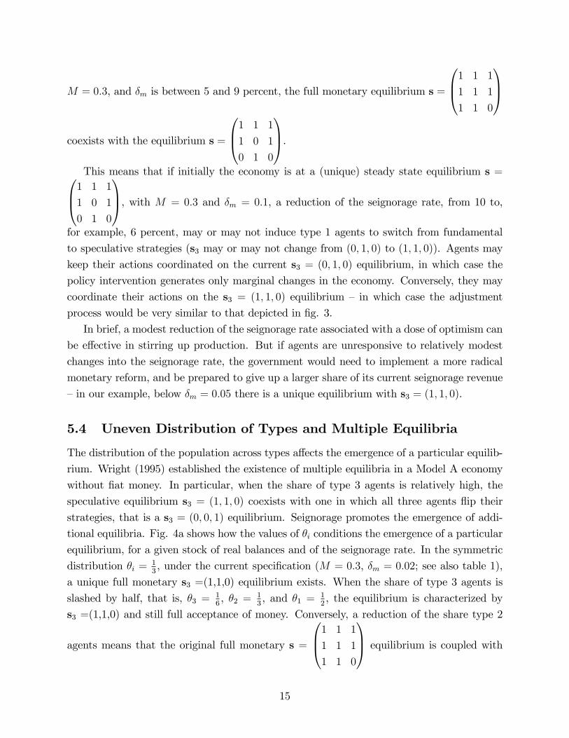
5.4 Uneven Distribution of Types and Multiple Equilibria
The distribution of the population across types a¤ects the emergence of a particular equilib-
rium. Wright (1995) established the existence of multiple equilibria in a Model A economy
without �at money. In particular, when the share of type 3 agents is relatively high, the
speculative equilibrium s3 = (1; 1; 0) coexists with one in which all three agents �ip their
strategies, that is a s3 = (0; 0; 1) equilibrium. Seignorage promotes the emergence of addi-
tional equilibria. Fig. 4a shows how the values of �i conditions the emergence of a particular
equilibrium, for a given stock of real balances and of the seignorage rate. In the symmetric
distribution �i = 13, under the current speci�cation (M = 0:3, �m = 0:02; see also table 1),
a unique full monetary s3 =(1,1,0) equilibrium exists. When the share of type 3 agents is
slashed by half, that is, �3 = 16, �2 = 1
3, and �1 = 1
2, the equilibrium is characterized by
s3 =(1,1,0) and still full acceptance of money. Conversely, a reduction of the share type 2
agents means that the original full monetary s =
0B@1 1 1
1 1 1
1 1 0
1CA equilibrium is coupled with
15
s =
0B@1 1 1
1 0 1
1 1 0
1CA. A unique equilibrium with partial acceptability of �at money is observed
when �1 is high and �3 is low �a situation in which type 2 easily trades 1 for 2.
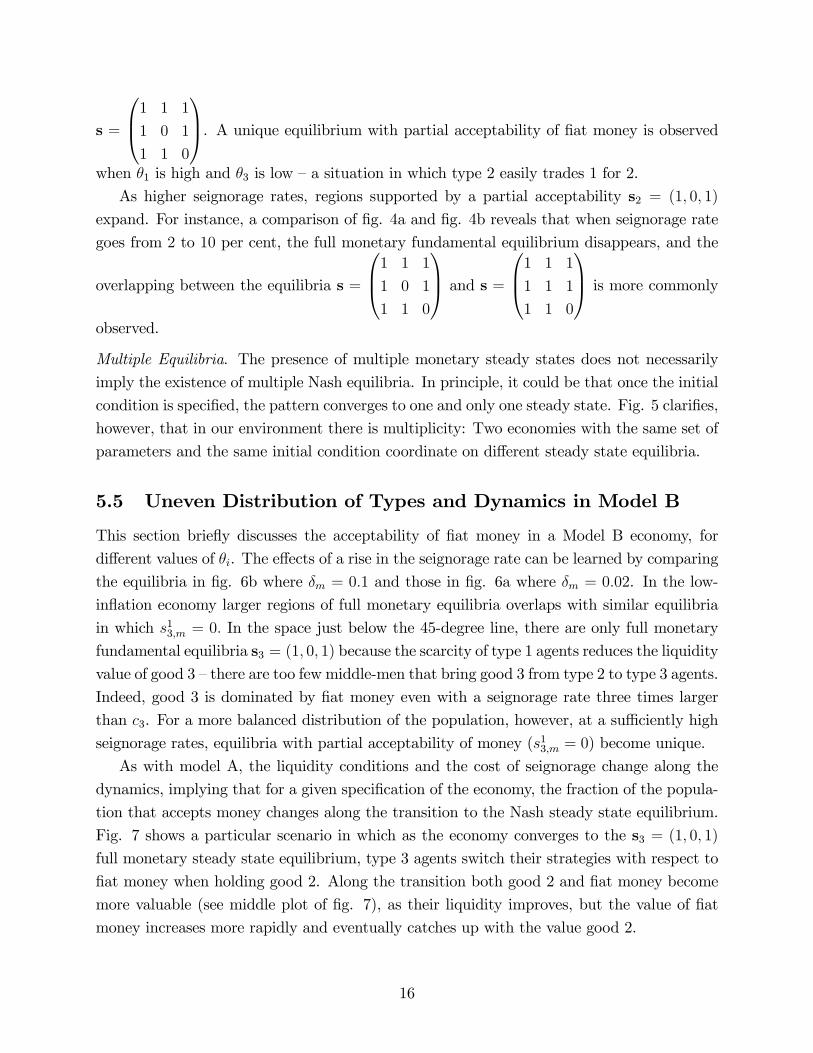
As higher seignorage rates, regions supported by a partial acceptability s2 = (1; 0; 1)
expand. For instance, a comparison of �g. 4a and �g. 4b reveals that when seignorage rate
goes from 2 to 10 per cent, the full monetary fundamental equilibrium disappears, and the
overlapping between the equilibria s =
0B@1 1 1
1 0 1
1 1 0
1CA and s =
0B@1 1 1
1 1 1
1 1 0
1CA is more commonly
observed.
Multiple Equilibria. The presence of multiple monetary steady states does not necessarily
imply the existence of multiple Nash equilibria. In principle, it could be that once the initial
condition is speci�ed, the pattern converges to one and only one steady state. Fig. 5 clari�es,
however, that in our environment there is multiplicity: Two economies with the same set of
parameters and the same initial condition coordinate on di¤erent steady state equilibria.
5.5 Uneven Distribution of Types and Dynamics in Model B
This section brie�y discusses the acceptability of �at money in a Model B economy, for
di¤erent values of �i. The e¤ects of a rise in the seignorage rate can be learned by comparing
the equilibria in �g. 6b where �m = 0:1 and those in �g. 6a where �m = 0:02. In the low-
in�ation economy larger regions of full monetary equilibria overlaps with similar equilibria
in which s13;m = 0: In the space just below the 45-degree line, there are only full monetary
fundamental equilibria s3 = (1; 0; 1) because the scarcity of type 1 agents reduces the liquidity
value of good 3 �there are too few middle-men that bring good 3 from type 2 to type 3 agents.
Indeed, good 3 is dominated by �at money even with a seignorage rate three times larger
than c3. For a more balanced distribution of the population, however, at a su¢ ciently high
seignorage rates, equilibria with partial acceptability of money (s13;m = 0) become unique.
As with model A, the liquidity conditions and the cost of seignorage change along the
dynamics, implying that for a given speci�cation of the economy, the fraction of the popula-
tion that accepts money changes along the transition to the Nash steady state equilibrium.
Fig. 7 shows a particular scenario in which as the economy converges to the s3 = (1; 0; 1)
full monetary steady state equilibrium, type 3 agents switch their strategies with respect to
�at money when holding good 2. Along the transition both good 2 and �at money become
more valuable (see middle plot of �g. 7), as their liquidity improves, but the value of �at
money increases more rapidly and eventually catches up with the value good 2.
16
6 Welfare
One standard question of monetary economics is whether the acceptance of �at money
improves the allocation of resources and stimulates production. The presence of matching
frictions and the assumption that agents incur a cost in holding commodities gives �at money
a potential positive role. Nevertheless, it also comes with costs at the individual�s and
society�s level. At the individual level, it looms the risk of con�scation. At the society level,
�at money reduces the availability of commodities �money chases away consumption goods.
To explores the welfare implications of introducing �at money and of altering seignorage
rates, we use, as KW, a utilitarian welfare criterion �given the highly symmetric type of
environment it is unlikely to observe a Pareto improvement from any given state. The payo¤
of a type i agent is calculated as a weighted average of Vi;j:
Wi(t) =1
�i(pi;i+1Vi;i+1 + pi;i+2Vi;i+2 + pi;mVi;m):
Therefore, the welfare of the whole society is simply the average of the three groups�payo¤s:
W (t) =Xi
�iWi(t).
As mentioned in the introduction the government derives utility from consuming goods.
These are purchased through the seignorage tax �mM . One may argue that the government
cares also about the welfare of the population. This could re�ect a genuine interest in
the society�s well-being, or more simply the desire of maintaining the population�s electoral
support. The government welfare function is then
WG(t) = (1� �)Q(t) + �W (t);
where
Q(t) =M
Z +1
t
e��G(��t)�m(�)d�;
and where � weighs the society�s welfare in the government�s objective function. For the
sake of the illustration, we consider an altruistic government (� = 1) that wants to know
how the level of M or the rate of seignorage a¤ects the population.
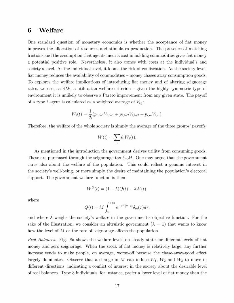
Real Balances. Fig. 8a shows the welfare levels on steady state for di¤erent levels of �at
money and zero seignorage. When the stock of �at money is relatively large, any further
increase tends to make people, on average, worse-o¤ because the chase-away-good e¤ect
largely dominates. Observe that a change in M can induce W1; W2 and W3 to move in
di¤erent directions, indicating a con�ict of interest in the society about the desirable level
of real balances. Type 3 individuals, for instance, prefer a lower level of �at money than the
17
other two groups. As they carry the low storage cost good, relative to the other two groups,
they are more preoccupied by the displacement of commodities caused by a further increase
in �at money than pleased by the savings in storage costs.
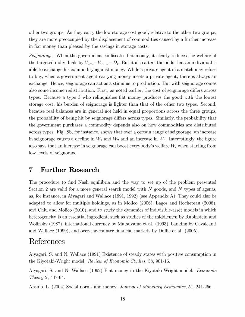
Seigniorage. When the government con�scates �at money, it clearly reduces the welfare of
the targeted individuals by Vi;m�Vi;i+1�Di. But it also alters the odds that an individual is
able to exchange his commodity against money. While a private agent in a match may refuse
to buy, when a government agent carrying money meets a private agent, there is always an
exchange. Hence, seignorage can act as a stimulus to production. But with seignorage comes
also some income redistribution. First, as noted earlier, the cost of seignorage di¤ers across
types: Because a type 3 who relinquishes �at money produces the good with the lowest
storage cost, his burden of seignorage is lighter than that of the other two types. Second,
because real balances are in general not held in equal proportions across the three groups,
the probability of being hit by seignorage di¤ers across types. Similarly, the probability that
the government purchases a commodity depends also on how commodities are distributed
across types. Fig. 8b, for instance, shows that over a certain range of seignorage, an increase
in seignorage causes a decline in W1 and W2 and an increase in W3. Interestingly, the �gure
also says that an increase in seignorage can boost everybody�s welfareWi when starting from
low levels of seignorage.
7 Further Research
The procedure to �nd Nash equilibria and the way to set up of the problem presented
Section 2 are valid for a more general search model with N goods, and N types of agents,
as, for instance, in Aiyagari and Wallace (1991, 1992) (see Appendix A). They could also be
adapted to allow for multiple holdings, as in Molico (2006), Lagos and Rocheteau (2008),
and Chiu and Molico (2010), and to study the dynamics of indivisible-asset models in which
heterogeneity is an essential ingredient, such as studies of the middlemen by Rubinstein and
Wolinsky (1987), international currency by Matsuyama et al. (1993), banking by Cavalcanti
and Wallace (1999), and over-the-counter �nancial markets by Du¢ e et al. (2005).
ReferencesAiyagari, S. and N. Wallace (1991) Existence of steady states with positive consumption in
the Kiyotaki-Wright model. Review of Economic Studies, 58, 901-16.
Aiyagari, S. and N. Wallace (1992) Fiat money in the Kiyotaki-Wright model. Economic
Theory 2, 447-64.
Araujo, L. (2004) Social norms and money. Journal of Monetary Economics, 51, 241-256.
18
Araujo, L., Camargo B., Minetti R, and Puzzello D. (2012) The essentiality of money in
environment with centralized trade. Journal of Monetary Economics, 59, 612-621.
Basçi, E. (1999) Learning by imitation. Journal of Economic Dynamics and Control, 23(9-
10), 1569-1585.
Baumol, W. (1952) The transactions demand for cash: An inventory theoretic approach.
The Quarterly Journal of Economics, 66(4), 545-556.
Brown, P. M. (1996) Experimental evidence on money as a medium of exchange. Journal of
Economic Dynamics and Control, 20(4), 583-600.
Brunner, M. and H. Strulik (2002) Solution of perfect foresight saddlepoint problems: A
simple method and applications. Journal of Economic Dynamics and Control, 26(5), 737-
53.
Cavalcanti, R. O. and N. Wallace (1999) Inside and outside money as alternative media of
exchange. Journal of Money, Credit and Banking, 31 (3), 443-457.
Chiu, J. and M. Molico (2010) Liquidity, redistribution, and the welfare cost of in�ation.
Journal of Monetary Economics, 57(4), 428-38.
Deviatov, A. and Wallace, N. (2014) Optimal in�ation in a model of inside money. Review
of Economic Dynamics, 17, 287�293.
Diamond, P. (1982) Aggregate demand management in search equilibrium. Journal of Po-
litical Economy, 90, 881-94.
Du¢ e, D., N. Gârleanu and L. Pederson (2005) Over-the-counter markets. Econometrica 73,
1815-1847.
Du¤y, J., and Jack Ochs (1999) Emergence of money as a medium of exchange: An experi-
mental study. American Economic Review, 89 (4), 847-877.
Du¤y, J., and Jack Ochs (2002) Intrinsically worthless objects as media of exchange: Exper-
imental evidence. International Economic Review, 43 (3), 637-674.
Goetzmann, W. N. (2016)Money changes everything: How �nance made civilization possible.
Princeton University Press.
Kehoe, M. J., N. Kiyotaki, and R. Wright (1993) More on money as a medium of exchange.
Economic Theory 3, 297-314.
Kiyotaki, N., and R. Wright (1989) On money as a medium of exchange. Journal of Political
Economy 97, 927�954.
Iacopetta, M. (2018) The emergence of money: A dynamic analysis. Macroeconomic Dy-
namics, forthcoming.
19
Jovanovic, B. (1982). In�ation and welfare in the steady state. Journal of Political Economy,
90, 561-77.
Lagos, R. and G. Rocheteau, (2009), Liquidity in markets with search frictions. Economet-
rica, 77(2), 403-26.
Lagos, R., G. Rocheteau, and R. Wright (2017) Liquidity: A new monetarist perspective.
Journal of Economic Literature 55, 371-440.
Li, V., (1994) Inventory accumulation in a search-based monetary economy. Journal of
Monetary Economics, 34, 511-36.
Li, V., (1995) The optimal taxation of �at money in search equilibrium. International
Economic Review, 36(4), 927-942.
Luo, G. (1999) The evolution of money as a medium of exchange. Journal of Economic
Dynamics and Control, 23, 415-58.
Mankiw, N. G., (2006) Principles of Economics, 4th ed., Cengage Learning.
Marimon, R., E. McGrattan, and T. Sargent (1990) Money as a medium of exchange in an
economy with arti�cially intelligent agents. Journal of Economic Dynamics and Control, 14,
329-73.
Matsuyama, K., N., Kiyotaki, and A. Matsui (1993) Toward a theory of international cur-
rency. Review of Economic Studies, 60(2), 283-307.
McGrattan, E.R., (1999) Application of weighted residual methods to dynamic economic
models. In: Marimon, R., Scott, A. (Eds.), Computational Methods For The Study Of
Dynamic Economies. Oxford University Press, Oxford, 114-142.
Molico, M. (2006) The distribution of money and prices in search equilibrium. International
Economic Review, 47(3), 701-22.
Mulligan, C. B. and X. Sala-i-Martin (1993) Transitional dynamics in two-sector models of
endogenous growth, The Quarterly Journal of Economics, 108(3), 739�773.
Nash, J. (1950) Equilibrium points in n-person games. Proceedings of the National Academy
of Sciences 36(1): 48-49.
Ober�eld, E. and T. Trachter (2012) Commodity money with frequent search. Journal of
Economic Theory, 147, 2332-56.
Quiggin, A. H. (1949) A survey of primitive money: the beginning of currency. Barnes and
Noble, New York.
Renero, J.M. (1998) Unstable and stable steady-states in the Kiyotaki-Wright model. Eco-
nomic Theory 11, 275-294.
20
Robinson, C., R., (1995) Dynamical systems, stability, symbolic dynamics, and chaos. Studies
in Advanced Mathematics, CRC Press, Boca Raton.
Rubinstein, A. and A. Wolinsky (1987) Middlemen. Quarterly Journal of Economics, 102,
581-94.
Shevchenko, A. and R. Wright (2004) A simple search model of money with heterogeneous
agents and partial acceptability. Economic Theory, 24(4), 877-885.
Sethi, R. (1999) Evolutionary stability and media of exchange. Journal of Economic Behavior
and Organization, 40, 233-54.
Tobin, J (1956) The interest elasticity of transactions demand for cash. The Review of
Economics and Statistics, 38(3), 241�47.
Wright, R. (1995) Search, evolution, and money. Journal of Economic Dynamics and Con-
trol, 19, 181-206.
21
A Proofs and derivations
This Appendix contains the proofs of Propositions 1 to 5. From the proofs of Propositions
1, 2, 4, and 5 it will emerge that their statements apply to a more general setting with N
objects and N types of agents. Speci�cally, the size of the matrix Ai, de�ned in (25) inthis Appendix, can be augmented to consider more objects, and the index i, associated with
types of individuals, can run up to an N > 3.
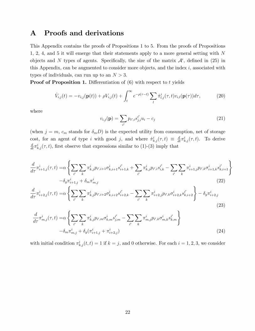
Proof of Proposition 1. Di¤erentiation of (6) with respect to t yields
_Vi;j(t) = �vi;j(p(t)) + �Vi;j(t) +Z 1
t
e��(��t)Xl
_�il;j(�; t)vi;l(p(�))d� , (20)
where
vi;j(p) =Xi0
pi0;isi0
j;iui � cj (21)
(when j = m, cm stands for �mD) is the expected utility from consumption, net of storage
cost, for an agent of type i with good j, and where _�ik;j(�; t) � ddt�ik;j(�; t). To derive
ddt�ik;j(�; t), �rst observe that expressions similar to (1)-(3) imply that
d
d��ii+1;j(�; t) =�
(Xi0
Xk
�ik;jpi0;i+1�ik;i+1s
i0
i+1;k +Xi0
�ik;jpi0;isi0
i;k �Xi0
Xk
�ii+1;jpi0;k�ii+1;ks
i0
k;i+1
)��g�ii+1;j + �m�im;j (22)
d
d��ii+2;j(�; t) =�
(Xi0
Xk
�ik;jpi0;i+2�ik;i+2s
i0
i+2;k �Xi0
Xk
�ii+2;jpi0;k�ii+2;ks
i0
k;i+2
)� �g�ii+2;j
(23)
d
d��im;j(�; t) =�
(Xi0
Xk
�ik;jpi0;m�ik;ms
i0
j;m �Xi0
Xk
�im;jpi0;k�im;ks
i0
k;m
)��m�im;j + �g(�ii+1;j + �ii+2;j) (24)
with initial condition �ik;j(t; t) = 1 if k = j, and 0 otherwise. For each i = 1; 2; 3, we consider
22
the 3� 3 matrix Ai =�Aij;k
j;k=i+1;i+2;m
de�ned as:
Aii+1;i+1 =� �Xi0
Xk 6=i+1
pi0;k�ii+1;ks
i0
k;i+1 � �g
Aii+1;i+2 =�Xi0
pi0;i+2�ii+1;i+2s
i0
i+2;i+1
Aii+1;m =�Xi0
pi0;m�ii+1;ms
i0
m;i+1 + �g
Aii+2;i+1 =�Xi0
pi0;i+1�ii+2;i+1s
i0
i+1;i+2 + �Xi0
pi0;isi0
i;i+2
Aii+2;i+2 =� �Xi0
Xk 6=i+2
pi0;k�ii+2;ks
i0
k;i+2 � �Xi0
pi0;isi0
i;i+2 � �g (25)
Aii+2;m =�Xi0
pi0;m�ii+2;ms
i0
m;i+2 + �g
Aim;i+1 =�Xi0
pi0;i+1�im;i+1s
i0
i+1;m + �Xi0
pi0;isi0
i;m + �m
Aim;i+2 =�Xi0
pi0;i+2�im;i+2s
i0
i+2;m
Aim;m =� �Xi0
Xk 6=m
pi0;k�im;ks
i0
k;m � �Xi0
pi0;isi0
i;m � �m :
The expressions in (22)-(24) then simplify to
d
d��ik;j(�; t) =
Xl
Ail;k(�)�il;j(�; t):
Observe that the matrix Ai satis�es Aij;k � 0 for j 6= k andXl
Aij;l = 0 ; (26)
for every j. These properties are used in proving Proposition 2 and Lemma 2 (see below).
Calling �i(�; t) the 3� 3 matrix with entries (�i)k;j(�; t) = �ik;j(�; t), the above equationcan be written as
d
d��i(�; t) = Ai(�)T�i(�; t) (27)
where Ai(t)T is the transpose of Ai(t). What is needed to compute the evolution of Vi;j(t),however, is the derivative of �i(�; t) with respect to t rather than with respect to � . Note,
however, that from (27) it follows that
�i(�; t� dt) = �i(�; t)�i(t; t� dt) = �i(�; t)�1 + dtAi(t)T
�:
23
Consequently,d
dt�i(�; t) = ��i(�; t)Ai(t)T ;
that in extended form becomes
d
dt�ik;j(�; t) = �
Xl
Aij;l(t)�ik;l(�; t). (28)
By inserting (28) in 20 we obtain
_Vi = �Vi �Ai(t)Vi � vi(t) (29)
where vi(t) = (vi;i+1(p(t)); vi;i+2(p(t)); vi;m(p(t))). Using the de�nition of the matrix Ai in(25) and of vi;j in (21) we get, for j = i+ 1 or i+ 2,
_Vi;j =�Vi;j � �(X
i0
Xk 6=i
pi0;k�ij;ks
i0
k;jVi;k +Xi0
pi0;isi0
i;jVi;i+1 �Xi0;k
pi0;k�ij;ks
i0
k;jVi;j
)��g(Vi;m � Vi;j)�
Xi0
pi0;isi0
j;iui + cj.
Rearranging terms we get:
_Vi;j =(�+ �g + �)Vi;j � �(X
i0
Xk 6=i
pi0;k�ij;ks
i0
k;jVi;k +Xi0
pi0;isi0
i;j(Vi;i+1 + ui)+
+Xi0;k
pi0;k(1� �ij;ksi0
k;j)Vi;j
)� �gVi;m + cj.
This is the expression in (7) when j = i+ 1 or j + 2. Similarly, when j = m
_Vi;m =�Vi;j � �(X
i0
Xk 6=i
pi0;k�im;ks
i0
k;mVi;k +Xi0
pi0;isi0
i;mVi;i+1 +Xi0;k
�im;ksi0
k;mVi;j
)��m(Vi;i+1 � Vi;m)�
Xi0
pi0;isi0
i;mui � �mDi =
=(�+ �g + �)Vi;m � �(X
i0
Xk 6=i
pi0;k�im;ks
i0
k;mVi;k +Xi0
pi0;isi0
i;m(Vi;i+1 + ui)+
+Xi0;k
(1� �im;ksi0
k;m)Vi;j
)+ �m(Vi;i+1 �Di).
This is expression in (7) for j = m.
Proof of Proposition 2. LetZ(t) = �(t; T )Z0 (30)
24
be the solution of the initial value problem8<: _Z = �Ai(t)ZZ(T ) = Z0 :
where Ai(t) is the matrix de�ned in (25). Consider now a variation of �ii+1;i+2(t) of the form
~�ii+1;i+2(t) = �ii+1;i+2(t) + ��(t):
where �(t) = 0 for t > T and � is a parameter. Di¤erentiating (29) with respect to � delivers
@� _Vi(t) = �@�Vi �Ai(t)@�Vi � @�Ai(t)Vi:
Using the property that @�Vi(t) = 0 if t > T , the Duhamel principle gives
@�Vi(t) =
Z T
t
e��(��t)�(t; �)@�Ai(�)Vi(�)d�:
From (25) it follows that
@�Ai(�)Vi(�)���=0= ���(�)�i
i+1;i+2(�)
0B@P
i0 pi0;i+2(�)si0i+2;i+1(�)
0
0
1CA :Therefore,
@�Vi(t)���=0=
Z 1
t
�(�)�ii+1;i+2(�)U(t; �)d� ,
where
U(t; �) = e��(��t)�(t; �)
0B@P
i0 pi0;i+2(�)si0i+2;i+1(�)
0
0
1CA .Equations (25) and (26) imply that �(t; �)i;j � 0 and �(t; �)i;i > 0. Moreover, because
pi+1;i+2(�) > 0 and si+1i+2;i+1(�) = 1, it follows that U(t; �)i+1 > 0 and that U(t; �)j � 0 forj = i+ 2;m.
Clearly, if�ii+1;i+2(�) 6= 0, the contribution of �(�) to the variation @�Vi(t) > 0 is di¤erent
than zero and there is no critical value for �1i+1:i+2(�) 2 (0; 1). We can then conclude Vi(t)
reaches a maximum at a boundary, i.e. �1i+1:i+2(�) 2 f0; 1g, and that
�ii+1;i+2(�) =
8<:1 �ii+1;i+2(�) < 0
0 �ii+1;i+2(�) > 0 :
(31)
Finally, as already observed in footnote 8 after Proposition 2, since�ii+1;i+2(t) = 0 for a �nite
set of switching times, the value of �ii+1;i+2(t) on such a set does not a¤ect Vi(t). Similar
observations hold for �ij;k with (j; k) 6= (i+ 1; i+ 2). This concludes the proof of (11).
25
Proof of Proposition 3. When M = �m = 0 the system (1)-(3) reduces to
_p1;2 = �fp1;3[p2;1(1� s23;1) + p3;1 + p3;2(1� s12;3)]� p1;2p2;3s12;3g; (32)
_p2;3 = �fp2;1[p3;2(1� s31;2) + p1;2 + p1;3(1� s23;1)]� p2;3p3;1s23;1g; (33)
_p3;1 = �fp3;2[p1;3(1� s12;3) + p2;3 + p2;1(1� s31;2)]� p3;1p1;2s31;2g: (34)
For a given pro�le of strategies, we need to check that the system (32)-(34) has a unique
globally attractive steady state.
Case (0,1,0). Eq. (34) reduces to _p3;1 = �(�3 � p3;1)(p1;3 + �2), implying that the planep3;1 = �3 is globally attractive. On this plane (32) reduces to _p1;2 = �(�1 � p1;2)�3, implyingthat the line p1;2 = �1, p3;1 = �3 is globally attractive. On this lines (33) becomes
_p2;3 = (�2 � p2;3)�1 � p2;3�3;
which clearly admits a unique globally attractive �xed point for p2;3 = �2�1�3+�1
. In brief,
under the pro�le of strategies (0,1,0), the distribution of inventories converges globally to
the stationary distribution (�1; �2�1�3+�1
; �3). For �i = 13this reduces to 1
3(1; 1
2; 1):
Case (1,1,0). Eq. 34 becomes _p3;1 = �(�3 � p3;1)�2. Consequently, the plane �3 = p3;1 isglobally attractive. The Jacobian, J , of the system of the two remaining eqs. 32 and 33 on
the plane �3 = p3;1 is
J = �
"�(�3 + p2;3) �p1;2(�2 � p2;3) �(�3 + p1;2)
#:
The determinant of J is always strictly positive, and its trace is always strictly negative;
therefore, both eigenvalues are negative for every relevant value of p1;2 and p2;3. Moreover
the set [0; �1]� [0; �2] is clearly positively invariant and compact. It thus follows easily fromthe Poincaré-Bendixon theorem that the system as a unique globally attractive �xed point.
To �nd the stationary distribution, set 32 and 33 to zero. They yield p1;2 = �1�3=(�3+p2;3)
and p1;2 = �3�2=p2;3�1 , respectively. The two lines necessarily cross once and only once for
p2;3 in the interval [0,�3]. The �xed point is (p�1;2; p�2;3; �3),where p
�2;3 =
12[�(�1 + �3) +p
(�1 + �3)2 + 4�1�2] and p�2;1 =�1�3
�3+p�2;3. When �i = 1
3the �xed point then is 1
3(p22;p2�1; 1).
Cases (1,0,1) and (0,1,1). A Jacobian with similar properties can be obtained when the
pro�les of strategies are (1,0,1) or (0,1,1). The �xed point with (1,0,1) is (p#1;2; �2; p#3;1), where
p#1;2 =12[�(�3 + �2) +
p(�3 + �2)2 + 4�3�1] and p
#3;1 =
�1�3p#1;2+�2
. Similarly, under (0,1,1), the
�xed point is (�1; �p2;3; �p3;2) where �p3;1 = 12[�(�2+�1)+
p(�2 + �1)2 + 4�2�3] and �p2;3 = �1�2
�p3;1+�1.
Using a similar argument on can verify that the �xed points supported by the strategies
(0,0,0), (0,0,1), and (1,0,0) are also stable.
26
Proof of Proposition 4. For � su¢ ciently small,
kp(0)� p�k � � implies kp(t)� p�k � C� 8t > 0 :
Since p� is a steady state, V�i must be a �xed point of (29), that is
�V�i �A�V�
i � v� = 0 (35)
where A� and v� are de�ned in (25) and (21) with p = p�. Calling �Vi(t) = Vi(t)�V�, by
subtracting (35) form (29) we get
_�Vi = ��Vi �A(t)�Vi �w(t)
where
w(t) = (A(t)�A�)V�i + (v(t)� v�):
From Lemma 2 below, it follows that
�Vi(t) = Vi(t)�V� =
Z t
1e�(t�s)�(t; s)w(s)ds:
Using that kw(t)k � C� we get that kVi(t)�V�i k = C� uniformly in t. Since (p�; s�) form a
Nash steady state, s� and V� must satisfy (11). It follows that Vi(t) and s� still satisfy (11)
if � is small enough. Thus, if kp(0)�p�k is small enough,s� is the best response to itself forall t > 0. It follows that (p(t); s�) is a Nash equilibrium.
Proof of Proposition 5. To prove the proposition, it is useful to state the stability
properties of (7). Let Vi(t; T;W) be the solution of (7) obtained by setting Vi(T; T;W) =
W.
Lemma 2 Given a set of strategies s(t) and �(t), and a pattern p(t), for anyW1 andW2:
kVi(t; T;W1)�Vi(t; T;W2)k1 � e��(T�t)kW1 �W2k1 (36)
where kUik1 = supj Ui;j, and t � T . Thus the value function at time t of agent ai can becomputed as
Vi(t) = limT!1
Vi(t; T;W) (37)
where the limit does not depend onW and it is reached exponentially fast.
Proof of Lemma 2. To obtain an explicit representation of Vi(t; T;W), we apply the
Duhamel principle to (29) and use the solution �(t; T ) of (30). So doing, we obtain
Vi(t; T;W) = e�(t�T )�(t; T )W +
Z t
T
e�(t��)�(t; �)v(�)d�; (38)
27

so that
Vi(t; T;W1)�Vi(t; T;W2) = e�(t�T )�(t; T )(W1 �W2) :
This implies
kVi(t; T;W1)�Vi(t; T;W2)k1 = e�(t�T )k�(t; T )k1kW1 �W2k1
The claim in Lemma 2 would hold if
k�(t; T )k1 � 1 8t � T : (39)
To prove (39) observe that
�(t; T ) = limN!1
1Yk=N
(1 + �tA(tk))
where
�t =T � tN
tk = t+ k�t:
Let C(tK) = 1 + �tA(tk). For �t small enough, Cl;j(tk) > 0 for every l; j andXj
Cl;j(tk) = 1 8l.
Therefore,
kC(tk)Wk1 = supl
�����Xj
Cl;jWj
����� � supl supj jWjjXj
jCl;jj = kWk1 :
Thus 39 is veri�ed because
k�(t; T )k1 � limN!1
1Yk=N
kC(tk)k1 � 1.
This completes the proof of Lemma 2.
Returning to Proposition 5, observe that Vi(t) = Vi(t; T;Vi(T )). From Lemma 2 we get
kVi(t)�Vi(t; T;V�i )k1 � e��(T�t)kVi(T )�V�
i k1:
Finally, to go from the in�nity distance kVi(t)�Vi(t; T;V�i )k1 to euclidean distance kVi(t)�
Vi(t; T;V�i )k we observe that for every W we have kWk1 � kWk �
p3kWk1. The
expression in Proposition 5 can thus be obtained as
kVi(t)�Vi(t; T;V�i )k �
p3kVi(t)�Vi(t; T;V
�i )k1 �
�p3e��(T�t)kVi(T )�V�
i k1 �p3e��(T�t)kVi(T )�V�
i k :
28
B Nash Equilibria and the Stable Manifold Theorem
The iteration procedure to �nd Nash equilibria is similar to that used by Perron to prove
the stable manifold theorem (for an illustration see, among others, Robinson, 1995). Here,
we discuss similarities and di¤erences. Consider the system of di¤erential equations8<: _x = ��x+ f�(x; y)_y = �y + f+(x; y)(40)
where x 2 Rn, y 2 Rm, �; � > 0 and
limjxj+jyj!0
jf�(x; y)j+ jf+(x; y)jjxj+ jyj = 0:
The system (40) is the sum of linear (��x and �y) and non-linear terms (f+ and f�); its�xed point is (x; y) = (0; 0).
The stable manifold theorem states that for every x0 2 Rn, with jx0j su¢ ciently small,there is unique y0 such that the solution (x(t); y(t)) of (40) starting at (x0; y0) satis�es
limt!1
(x(t); y(t)) = (0; 0): (41)
Moreover, it says that the point y0 is given by a smooth function of x0, that is y0 = W�(x0).
The graph of W�, that is the set (x0;W�(x0)), is called the local stable manifold of (0; 0).
Perron�s proof is based on the following representation of the solution of (40):
x(t) = e��tx0 +
Z t
0
e��(t��)f�(x(�); y(�))d� (42)
y(t) =
Z t
1e�(t��)f+(x(�); y(�))d�: (43)
The proof starts from a guess x0(t) = x0e��t and y0(t) = 0 for all t > 0. It then computes a
new approximation for the evolution of the stable variable x(t), x1(t), through (42). Inserting
x1 and y0 into (43) yields an approximation for the unstable variable y1(t). Note that while
in (42) time runs forward (� goes from 0 to t), in (43) it runs backward (in � goes from 1to t). Therefore both integrations are stable. Iterating the two steps just described yields
a sequence (xn(t); yn(t)) that approximates the solution (42)-(43). Because the exponential
factors in the integrals of (42) and (43) have negative exponents, if x0 is su¢ ciently small, the
map from (xn; yn) to (xn+1; yn+1) is a contraction. Finally, the Banach �xed-point theorem
guarantees that the sequence (xn(t); yn(t)) converges uniformly to a solution (x(t); y(t)) of
(40) with x(0) = x0 and satisfying (41).
There are similarities between Perron�s approach in proving the manifold theorem and the
construction of Nash equilibria discussed in Section 4. First, the Nash steady state (p�; s�)
29

corresponds to the �xed point (0; 0) of (40). Second, the p in (1)-(3) is comparable to the
x in (40). Third, in (38) the discount rate � plays the same role of the unstable exponent
� in (43). But there are also important di¤erences because. Fourth the value function Vi
in (7) is somewhat comparable to y in (40). But there is also an important di¤erence: The
value function Vi a¤ects the evolution of p through the intermediation of the strategies s.
In addition, di¤erently from (40), the procedure we presented in Section 4 does not split the
evolution of (p(t); s(t)) near (p�; s�) between a linear and a nonlinear part. Therefore, it is
better suited to follow the dynamics away form the steady state.
Finally, as noted in Section 4, it is important to recognize that the evolution of the
distribution of inventories, p(t), and that of the value functions V(t), can be studied jointly.
Starting from a p(T ) close to the steady state p�, with a Vi(T ) = V�i and �i(T ) = �
�i , one
may integrate (7) and (1)-(3) backward in time �t goes from T to 0. To �nd the approximate
solution of the Nash equilibrium it would su¢ ce to alter �i(t) along the integration process
so as to be consistent with the value functions Vi(t) � i.e. to satisfy (11). While this
procedure usually works well for low-dimensional systems (see, for instance, Brunner and
Strulik, 2002), it presents limitations for the type of research question we are after. Our
objective is to obtain a pattern (s(t);p(t)) that goes through any initial conditions, that
is, through any arbitrary points in the space of the distribution of inventories, p(0). As
the dimension of the manifold expands, guiding the system toward a particular point on
the state space by integrating (7) and (1)-(3) backward in time is challenging because some
regions of the manifold may be hard to reach. Conversely, the method proposed here o¤ers
total control over the initial condition, an indispensable feature for running macroeconomic
experiments.
30
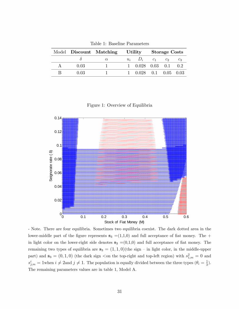
Table 1: Baseline Parameters
Model Discount Matching Utility Storage Costs� � ui Di c1 c2 c3
A 0.03 1 1 0.028 0.03 0.1 0.2
B 0.03 1 1 0.028 0.1 0.05 0.03
Figure 1: Overview of Equilibria
0 0.1 0.2 0.3 0.4 0.5 0.60
0.02
0.04
0.06
0.08
0.1
0.12
0.14
Stock of Fiat Money (M)
Seig
nora
te ra
te (
δ)
- Note. There are four equilibria. Sometimes two equilibria coexist. The dark dotted area in the
lower-middle part of the �gure represents s3 =(1,1,0) and full acceptance of �at money. The +
in light color on the lower-right side denotes s3 =(0,1,0) and full acceptance of �at money. The
remaining two types of equilibria are s3 = (1; 1; 0)(the sign �in light color, in the middle-upper
part) and s3 = (0; 1; 0) (the dark sign <on the top-right and top-left region) with s21;m = 0 and
sij;m = 1when i 6= 2and j 6= 1. The population is equally divided between the three types (�i = 13).
The remaining parameters values are in table 1, Model A.
31
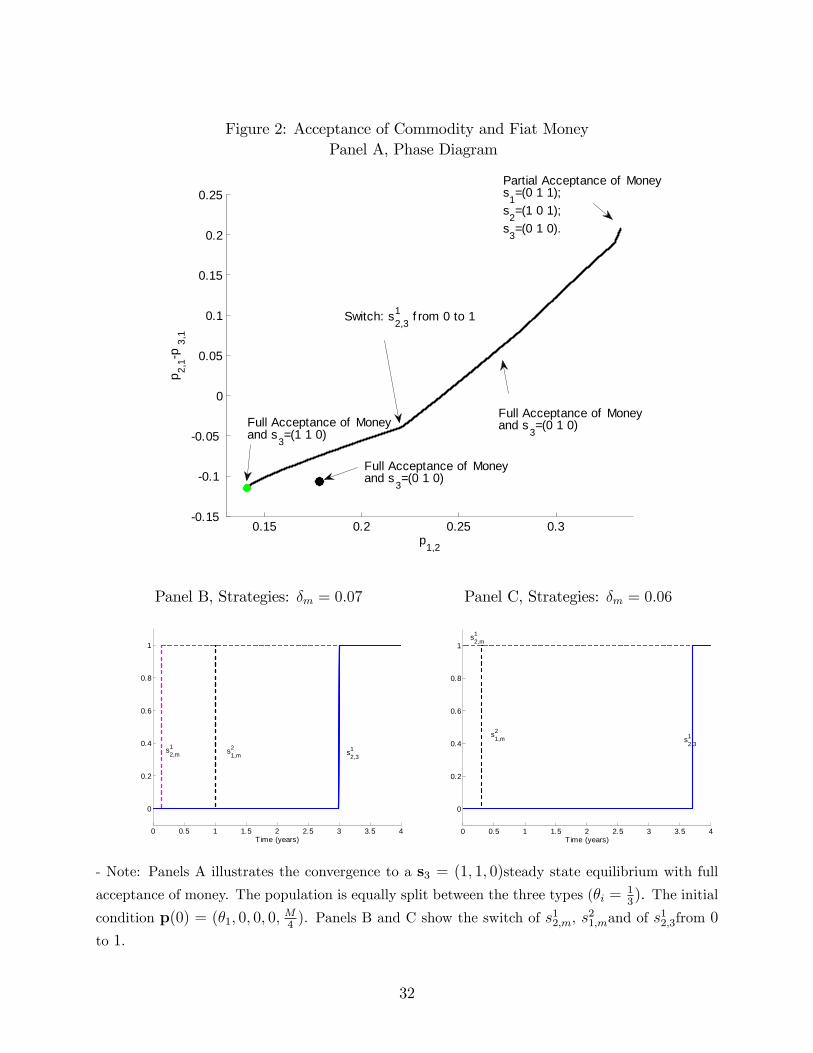
Figure 2: Acceptance of Commodity and Fiat MoneyPanel A, Phase Diagram
0.15 0.2 0.25 0.30.15
0.1
0.05
0
0.05
0.1
0.15
0.2
0.25
p 2,1p
3,1
p1,2
Switch: s12,3 f rom 0 to 1
Full Acceptance of Moneyand s3=(0 1 0)
Full Acceptance of Moneyand s3=(0 1 0)
Full Acceptance of Moneyand s3=(1 1 0)
Partial Acceptance of Moneys1=(0 1 1);s2=(1 0 1);s3=(0 1 0).
Panel B, Strategies: �m = 0:07 Panel C, Strategies: �m = 0:06
0 0.5 1 1.5 2 2.5 3 3.5 4
0
0.2
0.4
0.6
0.8
1
Time (years)
s12,m s2
1,m s12,3
0 0.5 1 1.5 2 2.5 3 3.5 4
0
0.2
0.4
0.6
0.8
1
Time (years)
s12,m
s21,m s1
2,3
- Note: Panels A illustrates the convergence to a s3 = (1; 1; 0)steady state equilibrium with full
acceptance of money. The population is equally split between the three types (�i =13). The initial
condition p(0) = (�1; 0; 0; 0;M4). Panels B and C show the switch of s12;m, s
21;mand of s
12;3from 0
to 1.
32
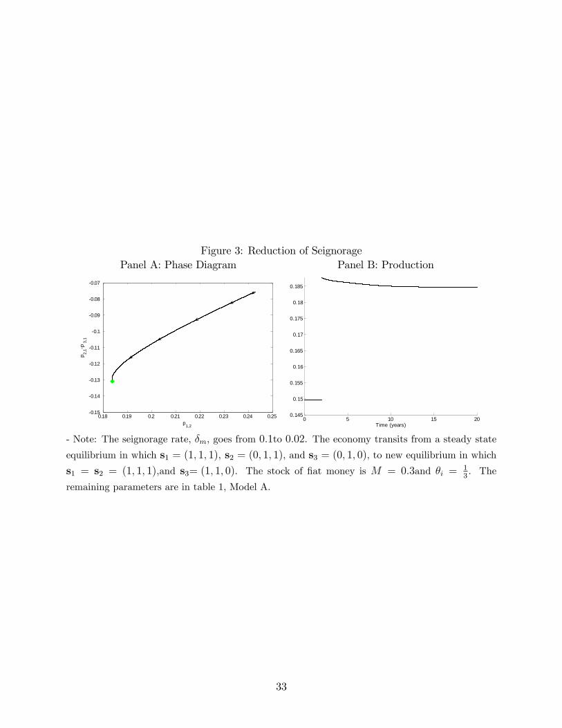
Figure 3: Reduction of SeignoragePanel A: Phase Diagram Panel B: Production
0.18 0.19 0.2 0.21 0.22 0.23 0.24 0.250.15
0.14
0.13
0.12
0.11
0.1
0.09
0.08
0.07
p 2,1p
3,1
p1,20 5 10 15 20
0.145
0.15
0.155
0.16
0.165
0.17
0.175
0.18
0.185
Time (years)
- Note: The seignorage rate, �m, goes from 0:1to 0:02. The economy transits from a steady state
equilibrium in which s1 = (1; 1; 1); s2 = (0; 1; 1), and s3 = (0; 1; 0), to new equilibrium in which
s1 = s2 = (1; 1; 1);and s3= (1; 1; 0). The stock of �at money is M = 0:3and �i =13. The
remaining parameters are in table 1, Model A.
33
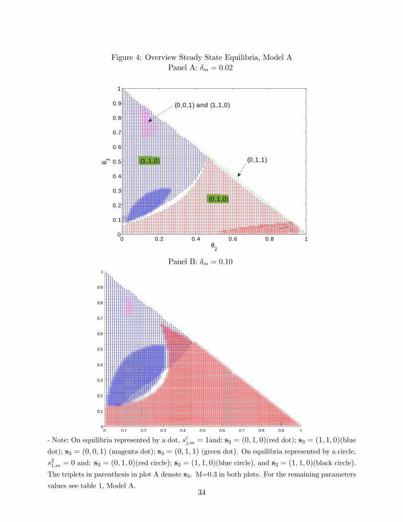
Figure 4: Overview Steady State Equilibria, Model APanel A: �m = 0:02
0 0.2 0.4 0.6 0.8 10
0.1
0.2
0.3
0.4
0.5
0.6
0.7
0.8
0.9
1
θ2
θ 3(0,0,1) and (1,1,0)
(1,1,0)
(0,1,0)
(0,1,1)
Panel B: �m = 0:10
0 0.1 0.2 0.3 0.4 0.5 0.6 0.7 0.8 0.9 10
0.1
0.2
0.3
0.4
0.5
0.6
0.7
0.8
0.9
1
- Note: On equilibria represented by a dot, sij;m = 1and: s3 = (0; 1; 0)(red dot); s3 = (1; 1; 0)(blue
dot); s3 = (0; 0; 1) (magenta dot); s3 = (0; 1; 1) (green dot). On equilibria represented by a circle,
s21;m = 0 and: s3 = (0; 1; 0)(red circle); s3 = (1; 1; 0)(blue circle), and s3 = (1; 1; 0)(black circle).
The triplets in parenthesis in plot A denote s3. M=0.3 in both plots. For the remaining parameters
values see table 1, Model A.34
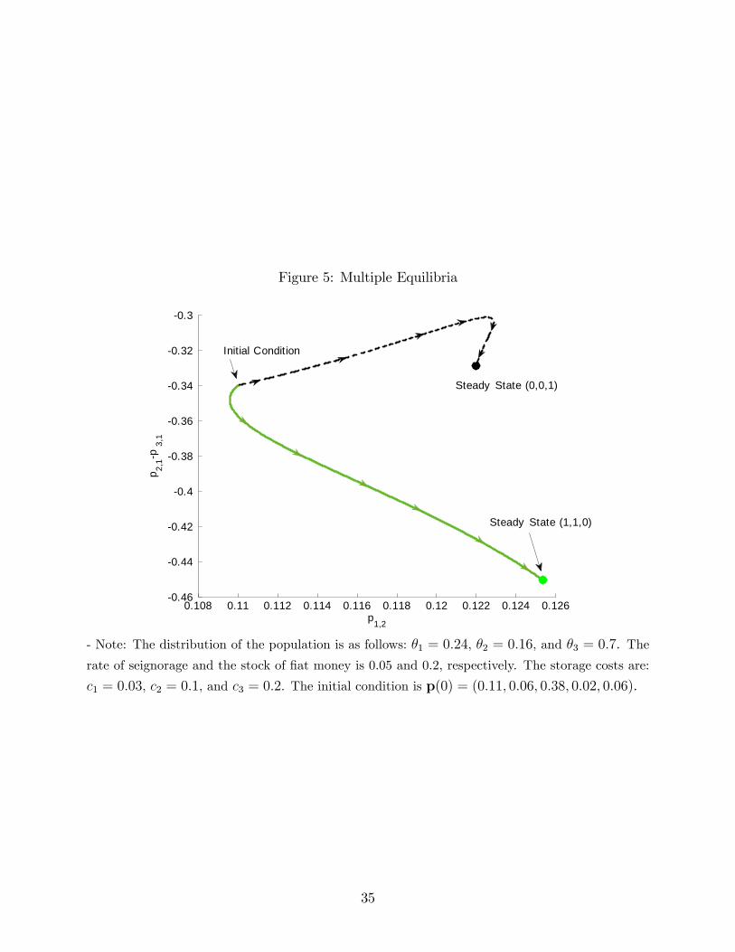
Figure 5: Multiple Equilibria
0.108 0.11 0.112 0.114 0.116 0.118 0.12 0.122 0.124 0.1260.46
0.44
0.42
0.4
0.38
0.36
0.34
0.32
0.3
p 2,1p
3,1
p1,2
Steady State (1,1,0)
Steady State (0,0,1)
Initial Condition
- Note: The distribution of the population is as follows: �1 = 0:24, �2 = 0:16, and �3 = 0:7. The
rate of seignorage and the stock of �at money is 0.05 and 0.2, respectively. The storage costs are:
c1 = 0:03, c2 = 0:1, and c3 = 0:2. The initial condition is p(0) = (0:11; 0:06; 0:38; 0:02; 0:06).
35
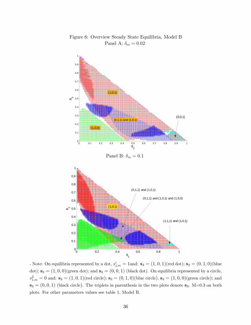
Figure 6: Overview Steady State Equilibria, Model BPanel A: �m = 0:02
0 0.1 0.2 0.3 0.4 0.5 0.6 0.7 0.8 0.9 10
0.1
0.2
0.3
0.4
0.5
0.6
0.7
0.8
0.9
1
θ2
θ 3
(1,0,1)
(1,0,0)
(0,0,1)(0,1,1) and (1,0,1)
Panel B: �m = 0:1
0 0.2 0.4 0.6 0.8 10
0.1
0.2
0.3
0.4
0.5
0.6
0.7
0.8
0.9
1
θ2
θ 3 (1,0,1)
(1,1,1) and (1,0,1)
(0,1,1) and (1,0,1)
(0,1,1) and (1,0,1) and (1,0,0)
- Note: On equilibria represented by a dot, sij;m = 1and: s3 = (1; 0; 1)(red dot); s3 = (0; 1; 0)(blue
dot); s3 = (1; 0; 0)(green dot); and s3 = (0; 0; 1) (black dot). On equilibria represented by a circle,
s21;m = 0 and: s3 = (1; 0; 1)(red circle); s3 = (0; 1; 0)(blue circle), s3 = (1; 0; 0)(green circle); and
s3 = (0; 0; 1) (black circle). The triplets in parenthesis in the two plots denote s3. M=0.3 on both
plots. For other parameters values see table 1, Model B.
36
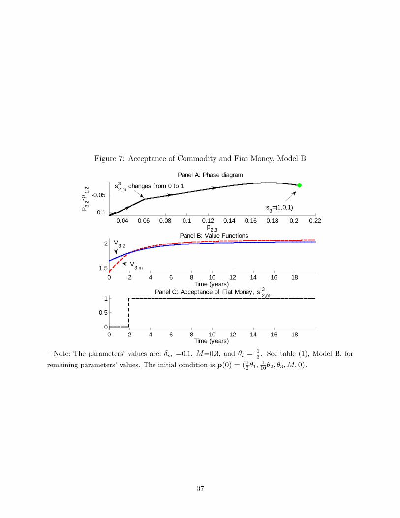
Figure 7: Acceptance of Commodity and Fiat Money, Model B
0.04 0.06 0.08 0.1 0.12 0.14 0.16 0.18 0.2 0.220.1
0.05
p 3,2p
1,2
p2,3
Panel A: Phase diagram
0 2 4 6 8 10 12 14 16 181.5
2
Time (years)
Panel B: Value Functions
0 2 4 6 8 10 12 14 16 180
0.5
1
Time (years)
Panel C: Acceptance of Fiat Money , s 32,m
V3,2
V3,m
s3=(1,0,1)
s32,m changes f rom 0 to 1
�Note: The parameters�values are: �m =0.1, M=0.3, and �i =13. See table (1), Model B, for
remaining parameters�values. The initial condition is p(0) = (12�1;
110�2; �3;M; 0).
37
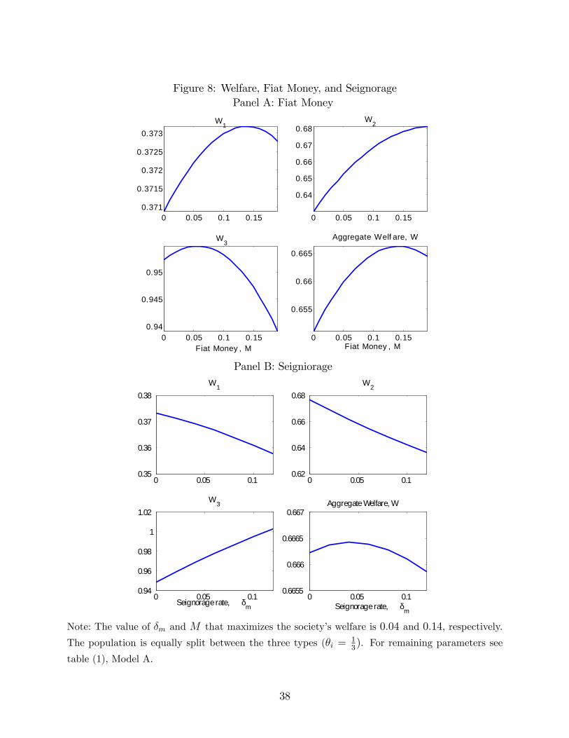
Figure 8: Welfare, Fiat Money, and SeignoragePanel A: Fiat Money
0 0.05 0.1 0.150.371
0.3715
0.372
0.3725
0.373W1
0 0.05 0.1 0.15
0.64
0.65
0.66
0.67
0.68W2
0 0.05 0.1 0.150.94
0.945
0.95
W3
Fiat Money , M0 0.05 0.1 0.15
0.655
0.66
0.665
Aggregate Welf are, W
Fiat Money , M
Panel B: Seigniorage
0 0.05 0.10.35
0.36
0.37
0.38W1
0 0.05 0.10.62
0.64
0.66
0.68W2
0 0.05 0.10.94
0.96
0.98
1
1.02
Seignorage rate, δm
W3
0 0.05 0.10.6655
0.666
0.6665
0.667Aggregate Welfare, W
Seignorage rate, δm
Note: The value of �m and M that maximizes the society�s welfare is 0:04 and 0:14, respectively.
The population is equally split between the three types (�i =13). For remaining parameters see
table (1), Model A.
38