ORIGINAL RESEARCH

A discrete particle swarm optimization algorithm with localsearch for a production-based two-echelon single-vendormultiple-buyer supply chain

Mehdi Seifbarghy1 • Masoud Mirzaei Kalani2 • Mojtaba Hemmati2

Received: 3 August 2014 /Accepted: 3 October 2015 / Published online: 4 November 2015

� The Author(s) 2015. This article is published with open access at Springerlink.com

Abstract This paper formulates a two-echelon single-

producer multi-buyer supply chain model, while a single

product is produced and transported to the buyers by the

producer. The producer and the buyers apply vendor-

managed inventory mode of operation. It is assumed that

the producer applies economic production quantity policy,

which implies a constant production rate at the producer.

The operational parameters of each buyer are sales quan-

tity, sales price and production rate. Channel profit of the

supply chain and contract price between the producer and

each buyer is determined based on the values of the

operational parameters. Since the model belongs to non-

linear integer programs, we use a discrete particle swarm

optimization algorithm (DPSO) to solve the addressed

problem; however, the performance of the DPSO is com-

pared utilizing two well-known heuristics, namely genetic

algorithm and simulated annealing. A number of examples

are provided to verify the model and assess the perfor-

mance of the proposed heuristics. Experimental results

indicate that DPSO outperforms the rival heuristics, with

respect to some comparison metrics.

Keywords Vendor-managed inventory � Economic

production quantity � Supply chain � Particle swarm

optimization

Introduction

A supply chain consists of a number of organizations with

materials, information and cash flows among them. Con-

sidering the first and last organizations as supplier and

customer, respectively, the chain’s objective is satisfying

customer requirements with optimal operational cost.

Vendor-managed inventory (VMI) as a modern IT-based

partnership technique has been of great attention in recent

years. In a VMI partnership, the supplier, usually the

manufacturer but sometimes a reseller or distributor, makes

the main inventory replenishment decisions for the con-

suming organization in such a way that the vendor moni-

tors the buyer’s inventory levels (physically or via

electronic messaging) and makes periodic replenishment

decisions.

This paper is an extension to Nachiappan and Jawahar

(2007) in which a two-echelon single-producer multi-buyer

supply chain (TSPMBSC) model while the vendor applies

economic production quantity (EPQ) instead of economic

order quantity (EOQ) is formulated. The producer and

buyers apply VMI mode of operation. The production rate

of the producer is assumed to be restricted. As an EOQ

inventory control system, the production is done during a

specific part of the replenishment cycle time. The buyers

are assumed to employ the well-known EOQ inventory

control system. The operational parameters are sales

quantity, sales price and the production rate for each buyer

which should be determined at the producer’s location.

Channel profit of the supply chain and contract price

& Mehdi Seifbarghy

seifbar@yahoo.com; m.seifbarghy@alzahra.ac.ir

Masoud Mirzaei Kalani

masood.mirzaie@gmail.com

Mojtaba Hemmati

mojtaba_h86@yahoo.com

1 Department of Industrial Engineering, Alzahra University,

Tehran, Iran

2 Faculty of Industrial and Mechanical Engineering, Qazvin

Branch, Islamic Azad University, Qazvin, Iran

123

J Ind Eng Int (2016) 12:29–43

DOI 10.1007/s40092-015-0126-6

between the producer and buyers is determined based on

the optimal values of the addressed operational parameters.

A mathematical programming model is developed to find

out the optimal values of the operational parameters. The

model has a nonlinear objective function involving several

integer variables and three different sets of linear con-

straints; it belongs to nonlinear integer programs (NIP).

Considering Govindan (2013) which researches on VMI

are classified into three categories of modeling, simulation,

and case studies, we can conclude that this paper falls into

the modeling category.

Costa and Oliveira (2001) addressed that the evolu-

tionary strategies such as genetic algorithm (GA) and

simulated annealing algorithm (SA) are emerging as the

best algorithms for solving NIP problems. GA and SA

could be useful for this NIP problem to provide near to

optimal solutions.

The revenue sharing and the partnership among mem-

bers of the supply chain are the major issues for the success

of a supply chain. The net revenue is addressed as channel

profit ‘Pc’ which depends on sales quantity. Sales quantity

is influenced by sales price (Waller et al. 2001). However,

the formulations would show that it depends on both sales

quantity and production rate while the vendor is also the

producer. The relationship between sales quantity and sales

price could be assumed to behave linearly (Lau and Lau

2003). It is generally believed that the pricing accept-

able (fair) to the partners involved is an important factor to

make constant relations in VMI, and that it requires

acceptable revenue sharing that would satisfy both the

vendor and the buyer (Grieger 2003). This reveals that the

revenue sharing between the vendor and the buyer plays a

vital role in determining the contract price.

The organization of the rest of the paper is as follows:

Sect. 2 is on the literature review, problem description and

modeling is given in Sect. 3. Section 4 gives the proposed

heuristics to solve the problem. In Sect. 5, a number of

numerical examples of different sizes are presented and

solved to measure the accuracy of the proposed heuristics.

Section 6 gives the research conclusions and ideas for

further research.

Literature review

The literature on two-echelon supply chains is rich enough.

Bhattacharjee and Ramesh (2000) developed two efficient

heuristics to derive the optimal price and ordering policies

to maximize the net profit of the retailer for a multi-period

inventory and pricing model. Lu (1995) pointed out that

future researches should consider the buyer’s point of view

and there should be a minimal acceptable profit level to

both the vendor and buyers; this made a suitable base for

the well-known concept which is revenue sharing. Maloni

and Benton (1997) stated that the major focus of revenue

sharing is to share the revenues/profits generated based on

the assignments and responsibilities to avoid the conflict

between supply chain partners. Yao and Chiou (2004)

considered the single-vendor and multi-buyer model pro-

posed by Lu (1995) and identified that the vendor’s optimal

annual cost function was a piecewise convex curve with

respect to the vendors’ production setup interval; they

suggested that a search algorithm can be developed to

obtain an optimal solution for a sub-problem. They also

proposed a search algorithm and demonstrated that their

algorithm reached a better result than Lu’s search

procedure.

Nachiappan and Jawahar (2007) formulated an inte-

grated inventory model of a two-echelon single-vendor

multiple buyers (TSVMBSC) under the VMI mode of

operation to maximize the channel profit and to share the

profit among the members involved assuming that both

vendors and buyers follow EOQ conditions. The given

model in this paper is an extension to the model given by

Nachiappan and Jawahar (2007) assuming that the entrance

rate of products to the vendor’s location is bounded (i.e.,

EPQ conditions); in the new formulation, the optimal

production rate for each buyer in the vendor’s (i.e., pro-

ducer’s) location is determined as well as the optimal sales

quantities and sales prices.

Zhang et al. (2007) presented an integrated VMI model

for a single vendor and multiple buyers, where the vendor

purchases and processes raw materials and then delivers

finished items to the buyers. A joint relevant cost model is

developed with constant production and demand rates

under the assumption that buyers’ ordering cycles may be

different and that each buyer can replenish more than once

in one production cycle. The main point of this research is

that demand rate at all buyers is constant while it is

determined as a function of the sales price in the current

research. Yao et al. (2007) developed an analytical model

that explores how important supply chain parameters affect

the cost savings to be realized from collaborative initiatives

as VMI. Van der Vlist et al. (2007) argue on the conclu-

sions drawn from Yao et al. (2007). They express that the

model ignores the costs of shipments from the supplier to

the buyer and plans the incoming and outgoing flows at the

supplier in a manner that overstates the inventory needed.

Toptal and Cetinkaya (2008) aimed to develop analyti-

cal and numerical results representing the system-wide cost

improvement rates which are due to coordination. Revis-

iting a few basic researches, they consider generalized

replenishment costs under centralized decision making.

This research analyzes (1) how the counterpart centralized

and decentralized solutions differ from each other, (2)

under what circumstances their implications are similar,

30 J Ind Eng Int (2016) 12:29–43

123

and (3) the effect of generalized replenishment costs of the

system-wide cost improvement rates which are subject to

coordination. Wang (2009) studied a decentralized supply

chain consisting of a single manufacturer and a single

distributor for a short lifecycle product with random yield

and uncertain demand as in the semiconductor industry.

Two scenarios for handling the business are considered.

One scenario is the traditional supply chain arrangement,

where the distributor is fully responsible for the inventory

decision, whereas the manufacturer is fully responsible for

the production decision. The other scenario is the VMI

arrangement, where the manufacturer is fully responsible

for the entire production and inventory decisions in the

supply chain. The optimal production and inventory deci-

sions under both scenarios are compared.

Yu et al. (2009a) discussed how the manufacturer

(vendor) can take advantage of the information received

from retailers for increasing his own profit using a Stack-

elberg game in a VMI system. The manufacturer produces

a finished product and supplies it at the same wholesale

price to multiple retailers. The retailers sell the product in

independent markets at retail prices. Solution procedures

are developed to find the Stackelberg game equilibrium

which each enterprise is not interested in deviating from

Yu et al. (2009b) investigated how a manufacturer and its

retailers cooperate each other to find their individual

optimal net profits considering product marketing (adver-

tising and pricing) and inventory policies in an informa-

tion-asymmetric VMI supply chain. The manufacturer

produces and gives a single product at the same wholesale

price to multiple retailers who sell the product in their

independent markets at retail prices. The manufacturer

determines its wholesale price, advertising investment,

replenishment cycles for the raw materials and finished

product, and backorder quantity to maximize the profit.

Retailers in turn consider the replenishment policies and

the manufacturer’s promotion policies and determine the

optimal retail prices and advertisement investments to

maximize their profits.

Zavanella and Zanoni (2009) investigated the way how a

particular VMI policy, known as Consignment Stock (CS),

may represent a successful strategy for both the buyer and

the supplier. The most radical application of CS may lead

to the suppression of the vendor inventory, as this actor

uses the buyer’s store to stock its finished products. As a

counterpart, the vendor will guarantee that the quantity

stored in the buyer’s store will be kept between a maximum

and a minimum level, also supporting the additional costs

eventually induced by stock-out conditions. The buyer will

pick up from its store the quantity of material needed to

meet its production plans and the material itself will be

paid to the buyer according to the agreement signed. Wong

et al. (2009) studied on how a sales rebate contract helped

to achieve supply chain coordination. For this purpose, a

model in the context of a two-echelon supply chain with a

single supplier serving multiple retailers in VMI partner-

ship is proposed. VMI facilitates the application of the

sales rebate contract since information sharing in VMI

partnership lets the supplier to obtain actual sales data in a

timely manner and determine the rebate for retailers. The

proposed model indicates that the supplier gains more

profit with competing retailers than without as competition

among the retailers lowers the prices and correspondingly

increases demand. Bichescu and Fry (2009) analyzed

decentralized supply chains, which followed continuous

review (Q, R) inventory policies considering VMI agree-

ments where the supplier chooses the order quantity Q, and

the retailer chooses the reorder point R. The effect of

divisions of channel power on supply chain and individual

agent performance is investigated by examining different

game theoretic models. The results showed that VMI can

result in considerable supply chain savings rather than

traditional relationships; furthermore, the greatest system

benefits from VMI arise in asymmetric channel power

relationships.

Almehdawe and Mantin (2010) consider a supply chain

consisting of a single capacitated manufacturer and mul-

tiple retailers. A Stackelberg game VMI framework under

two scenarios is utilized. Initially, the traditional approach

wherein the manufacturer is the leader is considered; in the

second, one of the retailers acts as the dominant player of

the supply chain. Darwish and Odah (2010) developed a

model for a supply chain with a single vendor and multiple

retailers under the VMI mode of operation. The developed

model can easily describe supply chains with capacity

constraints by selecting high penalty cost. Theorems are

given to tackle the complexity of the model. Furthermore,

an efficient algorithm is devised to find the global optimal

solution. Wang et al. (2010) investigate a recent paper by

Yao et al. (2007) and a critique by Van der Vlist et al.

(2007). Both researches presented interesting arguments to

show their valuable findings. However, their finding on the

buyer’s order sizes seems to conflict with each other.

Revisiting both papers, they come to the conclusion that

both papers are valid within the scopes and assumptions of

their own studies. Guan and Zhao (2010) considered a

single-vendor and a single-buyer supply chain and study

contracts for a VMI program. They design a revenue

sharing contract for vendor with ownership scenario, and a

franchising contract for retailer with ownership scenario.

Based on continuous review (R, Q) policy, without con-

sideration of order policy and related costs at the vendor

site, it is indicated that one contract can perform satisfac-

torily while the other one is a perfect contract. Considering

order policy and related costs at the vendor site, it is

indicated that one contract can perform satisfactorily while

J Ind Eng Int (2016) 12:29–43 31

123

the performance of the other one depends on the system

parameters. Bookbinder et al. (2010) consider a vendor,

which manufactures a single product sold to a retailer.

Three scenarios are studied: independent decision making

in which there is no agreement between the parties; VMI,

whereby the vendor initiates orders on behalf of the retai-

ler; and central decision making in which both vendor and

retailer are controlled by the same corporate entity. Opti-

mal solutions are obtained analytically for the retailer’s

order quantity, the vendor’s production quantity, the par-

ties’ individual and total costs in the three scenarios. Those

situations in which VMI is beneficial are recognized.

Razmi et al. (2010) considered a buyer–supplier supply

chain and compared the performance of the traditional and

VMI system using the total inventory cost of the supply

chain as the performance measure. The concept of extent

point is introduced in which the difference between the

total cost of both traditional and VMI systems is minimal.

It is applied to investigate how increasing or reducing the

key parameters changes the total cost of the two systems

with respect to each other. Goh and Ponnambalam (2010)

proposed a mathematical model to determine the optimal

sales quantity, optima sales price, optimal channel profit

and contract price between the vendor and buyer in

TSVMBSC under the VMI mode of operation. All the

parameters depend on the understanding of the revenue

sharing between the vendor and buyers. A particle swarm

optimization (PSO) was proposed to solve the problem.

The solutions obtained from PSO were compared with the

previous results reported in the literature. Pasandideh et al.

(2010) developed a model for a two-level supply chain

consisting of a single supplier and a single retailer studying

the inventory management practices before and after

implementation of VMI. This research explores the effect

of important supply chain parameters on the cost savings

realized from collaborative initiatives. The results indicate

that the VMI implementation of EOQ model when unsat-

isfied demand is backlogged sometimes has the ability to

reduce total costs of supply chains.

Pasandideh et al. (2011) developed an EOQ model for a

two-level supply chain consisting of one supplier and one

retailer in which unsatisfied demands are backordered, the

supplier’s storage is constrained and there is an upper

bound on the number of orders. They assume that the

supplier utilizes the retailer’s information in decision

making on the replenishments and supplies orders to the

retailer according to (R, Q) policy. A GA is proposed to

find the order quantities and the maximum backorder

levels, so that the total inventory cost of the supply chain is

minimized. Shao et al. (2011) studied inventory and pricing

policies in a non-cooperative supply chain with one sup-

plier and several retailers under an information-asymmetric

VMI environment. The supplier produces a product at the

wholesale price and gives to the retailers. The retailers

distribute the product in markets at retail selling prices. The

demand rate for each independent market is a non-de-

creasing concave function of the marketing expenditures of

both local retailers and the manufacturer, but a non-in-

creasing and convex function of the retail selling prices.

Wholesale price, marketing expenditure for supplier and

retailers, replenishment cycles for the product and backo-

rder quantity are determined in such a way as to maximize

the total profit. Sana et al. (2011) present an integrated

production-inventory model that is presented for supplier,

manufacturer and retailer supply chain, considering perfect

and imperfect quality items. This model considers the

impact of business strategies such as the optimal order size

of raw materials, production rate and unit production cost,

and idle times in different sectors on the collaborating

marketing system. An analytical method is employed to

optimize the production rate and raw material order size for

maximum expected average profit. An example is illus-

trated to study the behavior and application of the model.

Pal et al. (2012a, b) present a production inventory model

for various types of items where multiple suppliers, a

manufacturer and the multiple non-competing retailers are

the members of the supply chain. And each supplier sup-

plies only one type of raw material to the manufacturer.

The manufacturer produces a finished item by the combi-

nation of a certain percentage of the various types of raw

materials. The manufacturer produces also multi-items and

delivers them according to the demand of the different

retailers. Finally, an integrated profit of the supply chain is

optimized by optimal ordering lot sizes of the raw mate-

rials. A numerical example is provided to justify the pro-

posed model.

Pal et al. (2012a, b) develop a multi-echelon supply

chain model for multiple markets with different selling

seasons. Here, two suppliers are involved to supply the raw

materials to the manufacturer where the main supplier may

face supply disruption after a random time and the sec-

ondary supplier is perfectly reliable but more expensive

than the main supplier. In their article, the manufacturer

produces a random proportion of defective items which are

reworked after regular production and are sold in a lot to

another market just after completion of rework. The retailer

sells the finished products in different markets according to

seasons. Finally, an integrated expected cost per unit pro-

duct of the chain is minimized analytically by considering

the lot-size ordered as a decision variable. An appropriate

numerical example is also provided to justify the proposed

model. Goh et al. (2012) solved TSVMBSC model pro-

posed by Nachiappan and Jawahar (2007) utilizing PSO and

a hybrid of GA and artificial immune system (GA–AIS).

These two algorithms are evaluated for their solution quality

in the addressed research. Cardenas-Barron et al. (2012)

32 J Ind Eng Int (2016) 12:29–43

123

presented an alternative heuristic algorithm to solve the

vendor management inventory system with multi-product

and multi-constraint based on an EOQ model with autho-

rized stock out. Stock-out cost is considered linear and

fixed. Since the problem is a nonlinear integer program-

ming, a heuristic algorithm is proposed to solve the

problem.

Sadeghi et al. (2013) studied a multi-vendor multi-re-

tailer single-warehouse supply chain under the VMI mode

of operation with constrained space and annual number of

orders for the warehouse. The objective was to find the

order quantities along with the number of shipments

received by retailers and vendors in such a way as to

minimize the total inventory cost. Nia et al. (2013)

developed a multi-product EOQ model under a VMI policy

in a single-vendor single-buyer supply chain. Unsatisfied

demands are backordered. A few constraints such as stor-

age capacity, number of deliveries and order quantity are

considered in the given model. Demand, available storage

and total order quantity are considered as fuzzy numbers.

An ant colony optimization algorithm along with GA is

utilized to find a near-optimum solution. AriaNezhad et al.

(2013) attempts to develop the retailer’s inventory model

with the effect of order cancellations during the advance

sales period. The retailer announces a price discount pro-

gram during advance sales period to promote his sales and

also offers trade credit financing during the sales periods.

The retailer availing trade credit period from his supplier

offers a permissible delay period to his customers. The

customer who gets an item is allowed to pay on or before

the permissible delay period which is accounted from the

buying time rather than from the start period of inventory

sales. This accounts for significant changes in the calcu-

lations of interest payable and interest earned by the

retailer. The retailer’s total cost is minimized so as to find

out the optimal replenishment cycle time and price dis-

count policies through a solution procedure. The results

derived in mathematical theorems are implemented in

numerical examples, and sensitivity analyses on several

inventory parameters are obtained.

Diabat (2014) considered a two-echelon single-vendor

multi-buyer supply chain network operated under VMI

policy and found the optimal sales. Hybrid genetic/simu-

lated annealing algorithm is developed to deal with the

problem. Rad et al. (2014) considered a two-echelon sup-

ply chain consisting of a single vendor and two buyers. The

vendor gives a single product to both buyers at a finite

production rate. A mathematical model for the integrated

VMI policy is developed. Furthermore, solution algorithms

are proposed to determine the optimal lot size and total

inventory cost of the supply chain. The effect of key

parameters such as buyer’s demand and vendor’s holding

cost on lot size variation is also studied. Results show that

greater reduction in the total cost of the supply chain can be

obtained using VMI. Verma et al. (2014) proposed an

alternative replenishment scheme allowing for different

replenishment cycles for each retailer in the single-vendor

multi-retailer supply chain under VMI partnership. Talei-

zadeh and Noori-daryan (2014) considered a decentralized

three-layer supply chain including a supplier, a producer

and arbitrary number of retailers. Retailers order from the

producer who is replenished by the supplier. Demand is

assumed to be price sensitive. The paper optimizes the total

cost of the supply chain network integrating decision-

making policy using Stackelberg–Nash equilibrium. The

decision variables of the model are the supplier’s price, the

producer’s price and the number of shipments received by

the supplier and the producer. Pasandideh et al. (2014a)

studied single-vendor single-buyer supply chain system

under VMI working condition. The multiproduct EPQ

model considering backordering subject to the constraints

of storage capacity, number of orders, and available budget

was considered. The near optimal order quantities along

with the maximum backorder levels of the products in a

cycle are determined so that the total VMI inventory cost is

minimized. A GA-based heuristic is proposed to solve the

problem. Pasandideh et al. (2014b) present an integrated

vendor-managed inventory model for a two-echelon supply

chain organized as a single capacitated manufacturer at the

first echelon and multiple retailers at the second echelon.

Manufacturer produces different products whose demands

are assumed decreasing functions of retail prices. A fair

profit contract is designed for the manufacturer and the

retailers and the problem is formulated into a bi-objective

non-linear mathematical model. The lexicographic max–

min approach is utilized to obtain a fair non-dominated

solution.

Sana (2014) develops a production-inventory model of a

two-stage supply chain consisting of one manufacturer and

one retailer to study production lot size/order quantity,

reorder point sales teams’ initiatives where the demand of

the end customers is dependent on random variable and

sales teams’ initiatives simultaneously. The manufacturer

produces the order quantity of the retailer at one lot in

which the procurement cost per unit quantity follows a

realistic convex function of production lot size. In the

chain, the cost of sales team’s initiatives/promotion efforts

and wholesale price of the manufacturer are negotiated at

the points such that their optimum profits reached nearer to

their target profits. This study suggests to the management

of firms to determine the optimal order quantity/production

quantity, reorder point and sales teams’ initiatives/promo-

tional effort to achieve their maximum profits. An analyt-

ical method is applied to determine the optimal values of

the decision variables. Finally, numerical examples with its

graphical presentation and sensitivity analysis of the key

J Ind Eng Int (2016) 12:29–43 33

123

parameters are presented to illustrate more insights of the

model. In Sana et al. (2014), the replenishment size/pro-

duction lot size problem both for perfect and imperfect

quality products studied in their paper is motivated by the

optimal strategy in a three-layer supply chain consisting of

multiple suppliers, manufacturers and retailers. And each

manufacturer produces each product with a combination of

several raw materials which are supplied by each supplier.

The defective products at suppliers and manufacturers are

sent back to the respective upstream members at lower

price than the respective purchasing price. Finally, the

expected average profits of suppliers, manufacturers and

retailers are formulated by trading off setup costs, pur-

chasing costs, screening costs, production costs, inventory

costs and selling prices. The objective of this chain is to

compare between the collaborating system and Stakelberg

game structure so that the expected average profit of the

chain is maximized. In a numerical illustration, the optimal

solution of the collaborating system shows a better optimal

solution than the approach by Stakelberg. Thangam (2014)

in their paper attempts to develop the retailer’s inventory

model with the effect of order cancellations during the

advance sales period. The retailer announces a price dis-

count program during advance sales period to promote his

sales and also offers trade credit financing during the sales

periods. The retailer availing trade credit period from his

supplier offers a permissible delay period to his customers.

The customer who gets an item is allowed to pay on or

before the permissible delay period which is accounted

from the buying time rather than from the start period of

inventory sales. This accounts for significant changes in the

calculations of interest payable and interest earned by the

retailer. The retailer’s total cost is minimized so as to find

out the optimal replenishment cycle time and price dis-

count policies through a solution procedure. The results

derived in mathematical theorems are implemented in

numerical examples, and sensitivity analyses on several

inventory parameters are obtained.

Notation and modeling

The major notations used in this paper are as follows:

n Number of buyers

aj Intercept of the demand curve of buyer j

bj Slope of the demand curve of buyer j

Hbj Inventory holding cost of buyer j at the independent

mode (without VMI implementation)

Hs Inventory holding cost of the vendor (producer) at

the independent mode

HjVMIResultant inventory holding cost of the integrated

system of vendor and buyer j

Sbj Ordering (setup) cost of buyer j at the independent

mode

Ss Setup cost of the vendor per order at the

independent mode

SjVMIContinuously monitoring the stock status of buyer

j in VMI mode

P Total production rate of the vendor (producer)

hj Flow cost per unit from producer to buyer j

tj Transportation cost per unit delivered from vendor

to buyer j

d Production cost per unit made by the vendor

(producer)

PDj Production and distribution cost of products to

buyer j

PRj Revenue share ratio between vendor and buyer j

Qj Replenishment quantity for each buyer j

W Contract price between a vendor and a buyer

Wj Contract price between vendor and buyer j

Pj Production rate for buyer j at the vendor’s location

yj Sales quantity of buyer j

P(yj) Sales price of the product by buyer j corresponding

to sales quantity ‘yj’

P(y) Sales price of the product

yjminMinimum expected sales quantity of buyer j

yjmaxMaximum expected sales quantity of buyer j

This paper investigates a TSPMBSC model operating

under VMI mode.

Description of the demand curve and contract price

There are a lot of examples in practice in which each

producer (vendor) has its own set of direct outlets (distri-

bution centers/retailers addressed here as buyers). The

major parameters of the corresponding models are: sales

quantity ‘y’, the sales price at buyer’s market ‘P(y)’, the

contract price between the vendor and the buyer ‘W’ and

the production rate for each buyer at vendor location. The

sales quantity of the product at each location is highly

influenced by its sales price and it depends on the factors

such as the necessity of the commodity, the purchasing

power of the customers, and the nature of the product

(being perishable or storable). The general observation is

that the higher the sales price, the lower is the sales

quantity and vice versa. The relation between ‘P(y)’ and ‘y’

may be assumed to behave linearly and is given as

(Nachiappan and Jawahar 2007):

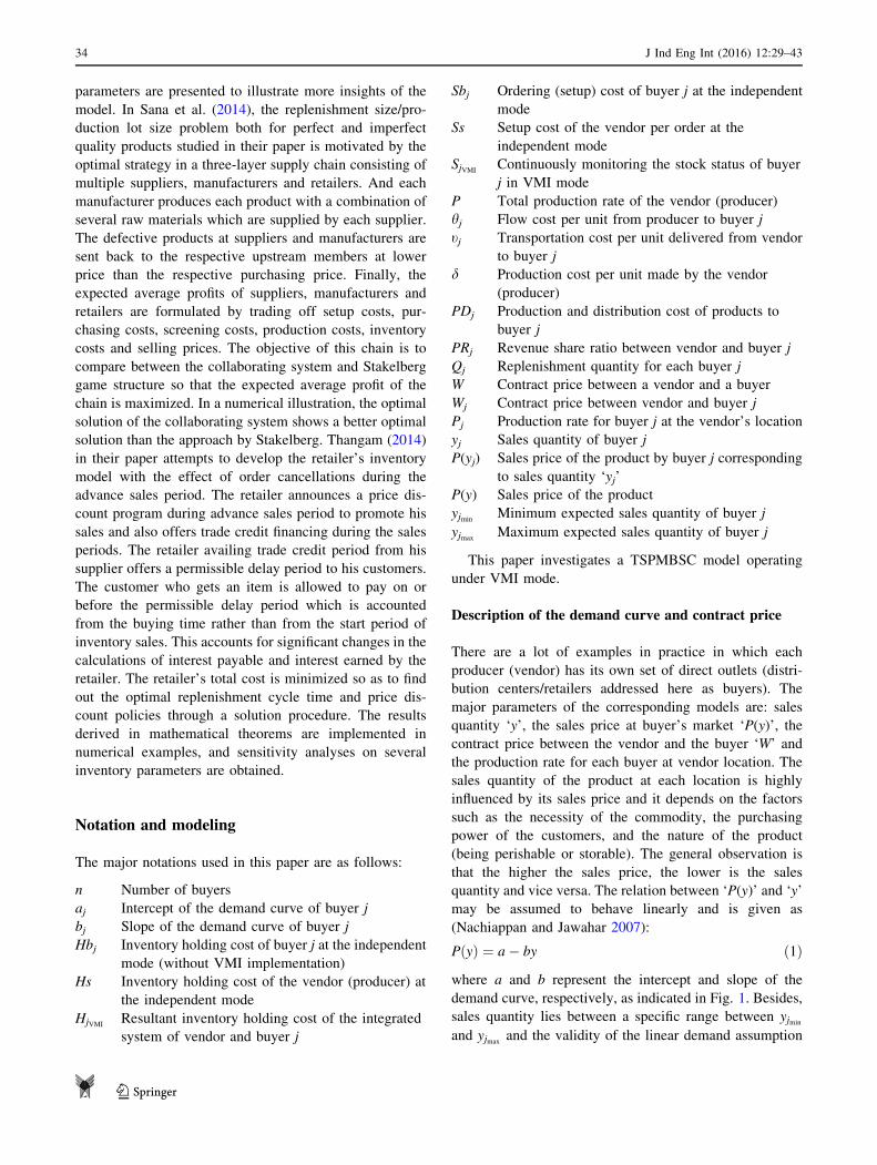
PðyÞ ¼ a� by ð1Þ

where a and b represent the intercept and slope of the

demand curve, respectively, as indicated in Fig. 1. Besides,

sales quantity lies between a specific range between yjmin

and yjmaxand the validity of the linear demand assumption

34 J Ind Eng Int (2016) 12:29–43

123

function holds very well within this range. Since the buyers

are not necessarily identical, the demand function of buyer

j may be stated as in (2)–(3)

PðyjÞ ¼ aj � bjyj ð2Þ

s:t: yjmin� yj � yjmax

ð3Þ

A parameter which plays an important role on the profits

of the both vendor and buyer(s) is the contract price. It is a

price which is mutually agreed between the vendor and the

buyer(s). Usually, it is assumed a value between the cost of

manufacturing and the sales price. The nature of the pro-

duct, the demand and the logistic cost play a critical role on

determination of the contract price value. The commodities

which have a good reputation and higher demand are

usually fast moving and are involved with lower risk; in

these circumstances, the buyer accepts the contract price

closer to sales price. However, in other cases where the

product is new and the demand is not yet stabilized, the

contract price is expected being settled at a lower level,

closer to the cost of manufacturing. In Nachiappan and

Jawahar (2007), the contract price is a variable which is

dependent on location, the competitiveness of the products,

the production and the operational costs between vendor

and buyer(s). The contract price between vendor and buyer

j is addressed by Wj.

Vendor operations and costs

Disney and Towill (2002) state that in VMI mode of

cooperation among the members of a vendor–buyers chain,

the vendor has more responsibility than the buyers and acts

as a leader. The vendor monitors, manages and replenishes

the inventory of all members (Achabal et al. 2000). The

associated costs include production cost, distribution cost,

order cost and stock holding cost. Production cost is

derived from the expenses spent for producing a single unit

‘d’ and the aggregate demand ‘y’ (i.e., y ¼Pn

j¼1 yj).

Therefore, the total production cost can be stated as dy. Thedistribution cost is the multiplication of flow and trans-

portation resource cost. The flow cost is the direct mileage

and the carrier contract cost per unit of buyer j ‘hj’ and the

transportation resource cost is the indirect cost such as

mode of transport, human router cost and administrative

costs and termed as ‘tj’ per unit demand for the buyer j

(Dong and Xu 2002). Therefore, the distribution cost can

be stated as ‘hjyjtjyj’. In this paper, it is assumed that the

products to all locations are delivered by road and the value

of ‘tj’ is taken as 0.5 per unit as Dong and Xu (2002)

consider. Therefore, the production and distribution costs

‘PDj’ to the vendor for meeting sales ‘yj’ of buyer j can be

given by (4)

PDj ¼ dyj þ 0:5hjy2j ð4Þ

The vendor monitors the stock status and replenishes the

stock. The buyer does not initiate orders. Therefore, the

order cost per replenishment ‘SjVMI’ associated with con-

tinuously monitoring the stock status is assumed as sum of

the order cost of vendor ‘Ss’ and order cost of buyer j ‘Sbj’

(Nachiappan and Jawahar 2007) and is given as in (5)

SjVMI¼ Ssþ Sbj ð5Þ

So, the cost involved with replenishing the batches ‘Qj’ of

demand of the buyer j ‘yj’ can be stated as ‘yj(Ss ? Sbj)/

Qj’. Nachiappan and Jawahar (2007) give this result in case

where the vendor’s production rate is infinite. However,

this is also valid while the production rate is finite.

The inventory is held at both the vendor and the buyer(s)

locations; the cost of holding one unit per unit time at

vendor and buyer j locations can be represented by ‘Hs’

and ‘Hbj’, respectively. The vendor accumulates inventory

before delivery to buyer ‘j’. As EPQ model, the vendor

holds an average inventory of ‘Qjð1� yjPjÞ=2’ to replenish

buyer j. The inventory held at the vendor to replenish buyer

j is given to the buyer. The average inventory at the buyer

location turns out to be ‘Qjð1� yjPjÞ=2’; this is why the

members use the VMI mode of cooperation. Therefore, in

VMI mode, the cost of holding inventory ‘HjVMI’ becomes

the sum of the inventory holding cost at vendor and buyer

(Nachiappan and Jawahar 2007); it can be given as in (6).

HjVMI¼ Hsþ Hbj ð6Þ

The sum of the order cost and average inventory holding

cost of the vendor for buyer ‘j’ namely ‘OSMj’, thus can be

stated as in (7):

OSMj ¼ ðSsþ SbjÞyj=QjþQjðHsþHb

jÞð1� yj=PjÞ=2 ð7Þ

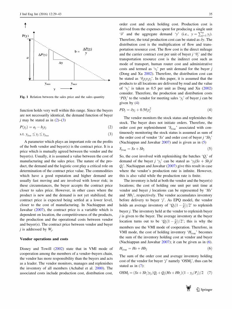
Fig. 1 Relation between the sales price and the sales quantity

J Ind Eng Int (2016) 12:29–43 35

123

Since the vendor produces for each buyer, assuming a

common cycle time ‘T’ for different buyers, the common

cycle time can be indicated as T ¼ Qj

yj; 8j ¼ 1; . . .; n (Silver

et al. 1998). The sum of order and average inventory

holding costs of the vendor for all buyers ‘OSM’ can be

stated as in (8)

OSM¼Xn

j¼1

½ðSsþSbjÞ=TþðHsþHbjÞ �T �yjð1� yj=PjÞ=2�;

ð8Þ

where ‘T’ is computed as:

T ¼

ffiffiffiffiffiffiffiffiffiffiffiffiffiffiffiffiffiffiffiffiffiffiffiffiffiffiffiffiffiffiffiffiffiffiffiffiffiffiffiffiffiffiffiffiffiffiffiffiffiffiffiffiffiffiffiffiffiffiffi2Pn

j¼1 ðSsþ SbjÞPn

j¼1 yjðHsþ HbjÞð1� yj=PjÞ

s

ð9Þ

The profit of the vendor when supplying the product to

buyer j ‘PVj’ can be obtained from the difference between

revenue to the vendor (Wjyj) and the total cost involved

‘PDj ? OSMj’. Therefore, the total profit to the vendor

‘PV’ by supplying its products to all the buyers can be

obtained from (10)

PV ¼Xn

j¼1

fWjyj � ðdyj þ 0:5hjy2j Þ � ½ðSsþ SbjÞ=T

þðHsþ HbjÞ � T � yjð1� yj=PjÞ=2�gð10Þ

Buyer operations and costs

As Nachiappan and Jawahar (2007) declare, the costs

associated with the buyers in VMI mode are the sales price

and the contract price. The sales price for each buyer is

determined using Eq. (2). The acceptable contract prices

that would satisfy both the vendor and the buyer are derived

from the revenue share ratio ‘PRj’. Thus, the profit of buyer j

‘Pbj’ in VMI mode is equal to the difference between the

sales revenue and the cost of purchase as in (11).

Pbj ¼ PðyjÞyj �Wjyj ¼ ðaj � bjyjÞyj �Wjyj ð11Þ

For a pre-specified value of revenue share ratio ‘PRj =

PVj/Pbj’ between the vendor and buyer j, the contract price

can be stated as in (12).

where ‘T’ is computed as in (9).

Objective function

The objective function is considered as the maximization

of channel profit of the supply chain. The mathematical

expression of channel profit ‘PC’ can be stated as in

(13).

PC ¼ PV þXn

j¼1

Pbj

¼Xn

j¼1

fajyj � bjy2j � ðdyj þ 0:5hjy

2j Þ � ½ðSsþ SbjÞ=T

þðHsþ HbjÞ � T � yjð1� yj=PjÞ=2�g ð13Þ

Mathematical programming model

The optimal or near optimal sales quantity and production

rate for buyer j namely ‘yjopt ’ and ‘Pjopt ’ are obtainable from

the following mathematical model which maximizes the

channel profit namely ‘PC’.

MaxPC ¼Xn

j¼1

fajyj � bjy2j � ðdyj þ 0:5hjy

2j Þ

�½ðSsþ SbjÞ=T þ ðHsþ HbjÞ � T � yjð1� yj=PjÞ=2�gð14Þ

s:t : yjmin� yj � yjmax

; 8j ¼ 1; . . .; n ð15ÞXn

j¼1

Pj ¼ P ð16Þ

yj �Pj; 8j ¼ 1; . . .; n ð17Þ

yj � 0; Pj � 0; 8j ¼ 1; . . .; n ð18Þ

Constraint (15) gives the valid upper and lower bounds of

the sales quantity for the buyers. Constraint (16) guarantees

that the sum of the buyer’s production rates should be equal

to the total production rate. Constraint (17) guarantees that

the demand rate be less than the production rate for all the

buyers as in EPQ model. Constraint (18) represents that the

decision variables of the models should be non-nega-

tive.The optimal sales price ‘PðyjoptÞ’ can be obtained from

(19).

PðyjoptÞ ¼ aj � bjyjopt ð19Þ

Wj ¼ajyjPRj � bjy

2j PRj þ dyj þ 0:5hjy2j þ ½ðSsþ SbjÞ=T þ ðHsþ HbjÞ � T � yjð1� yj=PjÞ=2�

ð1þ PRjÞyj; ð12Þ

36 J Ind Eng Int (2016) 12:29–43

123

The acceptable contract price ‘Wjopt ’ is yielded by substi-

tuting the optimal sales quantity ‘yjopt ’ in Eq. (12); the

result is given as in (20).

where

Topt ¼

ffiffiffiffiffiffiffiffiffiffiffiffiffiffiffiffiffiffiffiffiffiffiffiffiffiffiffiffiffiffiffiffiffiffiffiffiffiffiffiffiffiffiffiffiffiffiffiffiffiffiffiffiffiffiffiffiffiffiffiffiffiffiffiffiffiffiffiffiffi2Pn

j¼1 ðSsþ SbjÞPn

j¼1 yjoptðHsþ HbjÞð1� yjopt=PjoptÞ

s

ð21Þ

Proposed heuristics

Particle swarm optimization

Particle swarm optimization (PSO) was introduced by Ken-

nedy and Eberhart (1995) as a population-based search algo-

rithm. PSO is motivated from the simulation of social

behavior of bird flocking. PSO uses a population of particles

that fly through the search space to reach an optimum. Opti-

mization with particle swarms has two major ingredients, the

particle dynamics and the particle information exchange. The

particle dynamics are derived from swarm simulations in

computer graphics, and the information exchange component

is inspired by social networks. These ingredients combine to

make PSO a robust and efficient optimizer of real-valued

objective functions (although PSO has also been successfully

applied to combinatorial and discrete problems). PSO is

accepted as a computational intelligent technique; the major

difference betweenPSOand otherwell-knownheuristics such

as GA and SA is that the society members are aware of the

other members’ situation or at least of the best member and

consider the obtained information in their decision making.

Since the members can remember their best situation during

the algorithm operations and always try to include this in their

decisionmaking, they can compensate immediately in case of

a bad decision making. Each member can search the corre-

sponding neighboring boundary without being worried about

worsening the situation. The degree of being influenced by

othermembers of thepopulation is determinedbya coefficient

called learning coefficient.

PSO is similar to GA in that the system is initialized

with a population of random solutions (called particle

position); however, unlike GA, each potential solution is

also assigned a randomized velocity and does not neces-

sarily need to be encoded. Each individual or potential

solution (i.e., particle) flies in the problem dimensional

space with a velocity which is dynamically adjusted

according to the flying experiences of its own and its

colleagues. Each particle is affected by three factors: its

own velocity, the best position it has achieved so far

called ‘pbest’ and the overall best position achieved by all

particles called ‘gbest’. A particle changes its velocity

based on the three addressed factors. Denoted by np the

number of particles in the population (here, we assume

p = 2n), Let Xti ¼ ½xti;1; xti;2; . . .; xti;2n� representing the

position value of particle i with respect to dimension j

(j = 1, 2, …, 2n) at iteration t. We define the velocity of

each particle as Vti ¼ ½vti;1; vti;2; . . .; vti;2n� while each mem-

ber of vti corresponds to each member of Xti . Let Pb

ti ¼

½pbti;1; pbti;2; . . .; pbti;2n� be the best solution which particle i

has obtained by iteration t, and let Ptg ¼

½ptg;1; ptg;2; . . .; ptg;2n� be the best solution obtained by iter-

ation t.

Solution representation is one of the important steps

while designing a PSO-based heuristic. The decision vari-

ables can be very good guidelines in this regard. In this

paper, the solutions are represented as a string of 2n

characters in which the first n characters represent the

buyers’ sales values and the second n characters represent

the production rates of the vendor as {(y1, …, yn,

p1, …, pn)|ymin B yi B ymax, yi B pi,P

pi B P}. Imagine

that there are three buyers whose sales values are uniformly

distributed as y1 * U[1600, 4800], y2 * U[700, 1400],

y3 * U[1200, 3600] and the production capacity of the

vendor is as P = 18,000. As the constraints of the model

we should have yi B pi,P3

i¼1 pi � 18; 000; the particle

length should be 2n = 6. Three random numbers should be

generated corresponding to y1, y2, y3 noting that ymin

B yi B ymax. As the solutions are continuous, they will

convert to the discrete solutions by random number gen-

eration in order to be usable in the problem. Table 1

illustrates a sample vector of particles Xti used by PSO

algorithm.

Wjopt ¼ajyjoptPRj � bjy

2joptPRj þ dyjopt þ 0:5hjy2jopt þ ½ðSsþ SbjÞ=Topt þ ðHsþ HbjÞ � Topt � yjoptð1� yjopt=PjoptÞ=2�

ð1þ PRjÞyjopt; ð20Þ

J Ind Eng Int (2016) 12:29–43 37

123

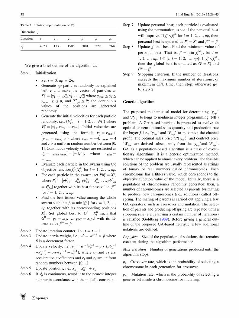
We give a brief outline of the algorithm as:

Step 1 Initialization

• Set t = 0, np = 2n.

• Generate np particles randomly as explained

before and make the vector of particles as

X0i ¼ ½y01; . . .; y0n; p01; . . .; p0n� where ymin B yi B

ymax, yi B pi andP

pi B P; the continuous

values of the positions are generated

randomly.

• Generate the initial velocities for each particle

randomly, i.e., fV0i ; i ¼ 1; 2; . . .;NPg where

V0i ¼ ½v0i;1; v0i;2; . . .; v0i;2n�. Initial velocities are

generated using the formula v0ij ¼ vmin þðvmax � vminÞ � r where vmin = -4, vmax = 4

and r is a uniform random number between [0,

1]. Continuous velocity values are restricted as

vtij ¼ ½vmin; vmax� ¼ ½�4; 4�, where vmin =

-vmax.

• Evaluate each particle in the swarm using the

objective function f 0i ðX0i Þ for i = 1, 2, …, np.

• For each particle in the swarm, set Pb0i ¼ X0i ,

where P0i ¼ ½pb0i;1 ¼ x0i;1; pb

0i;2 ¼ x0i;2; . . .; pb

0i;2n

¼ x0i;2n� together with its best fitness value, fpbi

for i = 1, 2, …, np.

• Find the best fitness value among the whole

swarm such that fl ¼ minff 0i g for i = 1, 2, …,

np together with its corresponding positions

X0l . Set global best to G0 ¼ X0

l such that

G0 = [g1 = xl,1, …, gDT = xl,2n] with its fit-

ness value fgb = fl.

Step 2 Update iteration counter, i.e., t = t ? 1

Step 3 Update inertia weight, i.e., wt = wt-1 9 b where

b is a decrement factor

Step 4 Update velocity, i.e., vtij ¼ wt�1vt�1ij þ c1r1ðpbt�1

ij

�xt�1ij Þ þ c2r2ðgt�1

j � xt�1ij Þ, where c1 and c2 are

acceleration coefficients and r1 and r2 are uniform

random numbers between [0, 1]

Step 5 Update positions, i.e., xtij ¼ xt�1ij þ vtij

Step 6 If xtij is continuous, round it to the nearest integer

number in accordance with the model’s constraints

Step 7 Update personal best; each particle is evaluated

using the permutation to see if the personal best

will improve. If f ti\fpbi for i = 1, 2, …, np, then

personal best is updated as Pti ¼ Xt

i and fpbi ¼ f ti

Step 8 Update global best. Find the minimum value of

personal best. That is, f tl ¼ minff pbi g, for i =

1, 2, …, np; l 2 {i; i = 1, 2, …, np}. If f ti \fgbi ,

then the global best is updated as Gt ¼ Xtl and

f gb ¼ f tlStep 9 Stopping criterion. If the number of iterations

exceeds the maximum number of iterations, or

maximum CPU time, then stop; otherwise go

to step 2.

Genetic algorithm

The proposed mathematical model for determining ‘yjopt ’

and ‘Pjopt ’ belongs to nonlinear integer programming (NIP)

problem. A GA-based heuristic is proposed to evolve an

optimal or near optimal sales quantity and production rate

for buyer j, i.e., ‘yjopt ’ and ‘Pjopt ’ to maximize the channel

profit. The optimal sales price ‘PðyjoptÞ’ and contract price

‘Wjopt ’ are derived subsequently from the ‘yjopt ’and ‘Pjopt ’.

GA as a population-based algorithm is a class of evolu-

tionary algorithms. It is a generic optimization method,

which can be applied to almost every problem. The feasible

solutions of the problem are usually represented as strings

of binary or real numbers called chromosomes. Each

chromosome has a fitness value, which corresponds to the

objective function value of the model. Initially, there is a

population of chromosomes randomly generated; then, a

number of chromosomes are selected as parents for mating

to produce new chromosomes (i.e., solutions) called off-

spring. The mating of parents is carried out applying a few

GA operators, such as crossover and mutation. The selec-

tion of parents and producing offspring are repeated until a

stopping rule (e.g., elapsing a certain number of iterations)

is satisfied (Goldberg 1989). Before giving a general out-

line of the proposed GA-based heuristic, a few additional

notations are defined:

Pop_size Size of the population of solutions that remains

constant during the algorithm performance.

Max_iteration Number of generations produced until the

algorithm stops.

pc Crossover rate, which is the probability of selecting a

chromosome in each generation for crossover.

pm Mutation rate, which is the probability of selecting a

gene or bit inside a chromosome for mutating.

Table 1 Solution representation of Xti

Dimension, j

Location y1 y2 y3 p1 p2 p3

xtij 4620 1333 1505 5801 2296 2640

38 J Ind Eng Int (2016) 12:29–43

123

Fitness_function Fitness function value, which exactly

corresponds to the objective function value in this paper.

We give a brief outline of the algorithm as:

Step 1 Initialization

• Set Pop_size, Max_iteration, pc and pm.

Step 2 Randomly generate the initial population

Step 3 Repeat until Max_iteration:

Step 3.1 Perform the reproductionoperator accord-

ing to the roulette wheel rule tomake a

new population

Step 3.2 Select the parent chromosomes from

the obtained population, each with

probability pcStep 3.3 Crossover:

(a) Determine the pairs of parents

among the parent chromosomes.

(b) Apply the crossover operator to

produce two offspring corre-

sponding to each pair.

(c) Replace each offspring in the

population instead of the

parents.

Step 3.4 Apply the mutation operator on the

population with probability pmStep 3.5 Calculate Fitness_function for each

chromosome and save the best value in

bv (best value)

Step 4 Print bv

Each chromosome consists of 2n genes. The first n genes

represent the sales quantities of the buyers and the second n

genes represent the production rates of them. As an

example, the chromosome [1 1 3 4 5 7 9 10] indicates that

there are four buyers whose sales quantities are 1, 1, 3 and

4, respectively, and production rates are 5, 7, 9 and 10,

respectively.

The Pop_size, pc and pm are determined through the try

and error method while Max_iteration is assumed equal to

2000.

Simulated annealing

SA proposed by Kirkpatrick et al. (1983) is a stochastic and

neighborhood-based search algorithm motivated from an

analogy between the simulation of the annealing of solids

and the strategy of solving combinatorial optimization

problems. SA has been widely applied to solve combina-

torial optimization problems as Yao (1995) declares. It is

inspired by the physical process of heating a substance and

then slowly cooling it, until a strong crystalline structure to

be formed. This process is simulated through gradually

lowering an initial temperature until the system reaches an

equilibrium point so that no more changes occur. Gener-

ally, details of SA proposed are as follows:

Algorithm: simulated annealing

1: Initialize parameters T0, N, K, a, Tf2: Initialized counter n = 0, k = 0

3: Do (outside loop)

4: Set n = 0

5: Generate initial solution X0 : Set XBest ¼ X0

6: Do (inside loop)

7: Generate neighboring solution Xn-1 by operation (Xn ? Xn-1)

8: If f(Xn?1) � f(Xn) then

9: Xn = Xn?1: Set n = n ? 1

10: Else

11: Generate random Rand ? u(0, 1)

12: If Rand\e�DF=Tk then Xn = Xn?1: set n = n ? 1

13: End if

14: Update XBest

15: Loop until (n B N)

16: Tr?1 = aTr17: Loop until frozen

Computational experiments

Nachiappan and Jawahar (2007) analyzed their proposed

model and methodology by a case study carried out at the

SNP dairy company located in Madurai, India. The dairy

manufacturer (vendor) supplies its product (milk packets)

to the customers at different locations (buyers). Since the

structure of our proposed model is near to that of Nachi-

appan and Jawahar (2007), we have provided a few

numerical problems inspiring from those of Nachiappan

and Jawahar (2007). The numerical problems are given in

three categories while considering three, five, and eight

buyers in the model. Since the number of parameters is too

much, the buyer-related parameters are considered fixed,

while the vendor-related parameters are changed in order to

do the sensitivity analysis. The values of the buyer-related

parameters are given in Table 2. Five problems are selec-

ted from each category as small, medium and large size

J Ind Eng Int (2016) 12:29–43 39

123

problems. The values of the vendor-related parameters are

given in Table 3.

In the rest of this section, we are going to compare the

proposed GA, discrete particle swarm optimization algo-

rithm (DPSO), and SA for TSVMBSC problem. We have

also used LINGO solver to assess the performance of the

proposed heuristics. All the heuristics are coded in Mat-

lab7.0 software and run on a PC with 1.67 GHz processor

(Intel Pentium 4), 256 MG memory and windows XP

Professional Operating System.

We have used relative percentage index (RPI) to assess

the performance of the proposed heuristics. This index is

one of the well-known indexes in this regard for single

objective problems. We have solved a number of instances

for each numerical problem. RPI can be computed by

Eq. (22) in which Maxsol and Worstsol represent the best

and worst objective function values obtained from solving

the instances of each numerical problem while solving it by

different heuristics; A lgsol represents the objective function

value for each instance of a numerical problem.

RPI ¼ Maxsol � A lgsolMaxsol �Worstsol

ð22Þ

RPI can take values between 0 and 1. Clearly, lower values

of RPI are preferred. Table 4 gives the RPI values for each

numerical problem while solving it by each heuristic as

well as using LINGO solver. We have considered the

number of instances for each numerical problem equal to

five times; the average of the obtained objective function

values from solving the five instances is considered as RPI

for each numerical problem with respect to each heuristic.

The CPU times are considered the same for the heuristics;

however, we have reported the CPU times when each

algorithm reached the best corresponding solution.

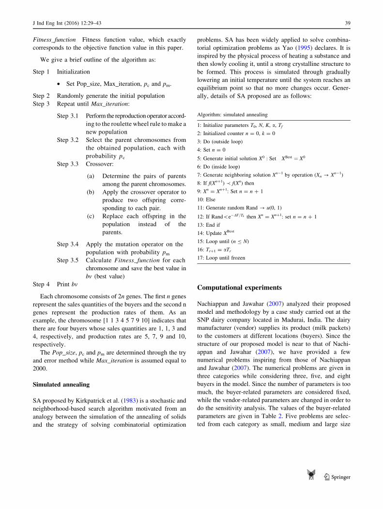
As it is clear from Table 4, the RPI for DPSO is less

than that of other heuristics; however, the average CPU

time of LINGO solver is less than that of other heuristics.

We have also used statistical t test at significance level

a = 0.05 to compare each heuristic with the other con-

sidering H0: D = 0 against H1: D[ 0 in which D repre-

sents the difference between the average of RPI of the first

heuristic and that of the second. Therefore, hypothesis H0

can be rejected if and only if t ¼ DSD=

ffiffin

p [ ta;n�1. Table 5

illustrates the results.

Figure 2 indicates the average value of LSD with con-

fidence interval 95 % for various heuristics. It is clear from

Fig. 2 that DPSO is superior compared with other heuris-

tics and LINGO solver.

Conclusions and suggestion

This paper presents a TSPMBSCmodel under theVMImode

of operation. It is the extension of Nachiappan and Jawahar

(2007) for the case where the vendor (producer) replenishes

orders as EPQ, i.e., the product gradually enters into the

vendor’s location. The final model can be stated as a math-

ematical programming model with the objective function of

channel profit and the two decision variables of sales quan-

tity and production rate. Thereafter, the optimal values of the

decision variables are determined. The aforementioned

problem is NP-hard which means too difficult to be solved

during a logical amount of time. We presented a DPSO-

based heuristic to solve the problem. To prove the efficiency

of the proposed heuristic, two distinct kinds of heuristics

were used, including innovative searching method of the

GA, and SA; however, LINGO solver was also used. The

heuristics applied to solve a set of small, medium and large

Table 2 Values of the buyer-related parameters

Buyer-related data for n = 3 Buyer-related data for n = 5 Buyer-related data for n = 8

j 1 2 3 1 2 3 4 5 1 2 3 4 5 6 7 8

Hbj 8 10 10 8 10 10 6 7 8 10 10 6 7 12 13 14

Sbj 24 11 29 24 11 29 14 25 24 11 29 14 25 12 30 22

aj 31 35 37 31 35 37 32 39 31 35 37 32 39 33 36 38

bj 0.008 0.004 0.006 0.008 0.004 0.006 0.003 0.004 0.008 0.004 0.006 0.003 0.004 0.005 0.007 0.006

yjmin1600 700 1200 1600 700 1200 1500 900 1600 700 1200 1500 900 700 800 1200

yjmax4800 1400 3600 4800 1400 3600 3000 2700 4800 1400 3600 3000 2700 3500 4900 3000

hj 0.004 0.008 0.005 0.004 0.008 0.005 0.005 0.007 0.004 0.008 0.005 0.005 0.007 0.005 0.007 0.006

Table 3 Values of the vendor-related parameters

Level Hs Ss d P

Low (-1) 3 5 5 18,000

Up (?1) 15 40 10 27,000

40 J Ind Eng Int (2016) 12:29–43

123

size problems. The results indicated that the DPSO excels

compared to the other rival heuristics.

Though the model considered in this paper is restricted

to two-echelons, further analysis is required to study the

performance under multi-echelon supply chains. Besides,

demand can be lost or backordered while it is stochastic.

Open Access This article is distributed under the terms of the

Creative Commons Attribution 4.0 International License (http://crea

tivecommons.org/licenses/by/4.0/), which permits unrestricted use,

distribution, and reproduction in any medium, provided you give

appropriate credit to the original author(s) and the source, provide a

link to the Creative Commons license, and indicate if changes were

made.

References

Achabal DD, Mcintyre SH, Smith SA, Kalyanam K (2000) A decision

support system for VMI. J Retail 76(4):430–454

Almehdawe E, Mantin B (2010) Vendor managed inventory with a

capacitated manufacturer and multiple retailers: retailer versus

manufacturer leadership. Int J Prod Econ 128(1):292–302

AriaNezhad MG, Makuieand A, Khayatmoghadam S (2013) Devel-

oping and solving two-echelon inventory system for perishable

items in a supply chain: case study (Mashhad Behrouz

Company). J Ind Eng Int. doi:10.1186/2251-712X-9-39

Bhattacharjee S, Ramesh R (2000) A multi-period profit maximizing

model for retail supply chain management: an integration of

demand and supply side mechanism. Eur J Oper Res

122:584–601

Bichescu BC, Fry MJ (2009) Vendor-managed inventory and the

effect of channel power. OR Spectr 31(1):195–228

Bookbinder JH, Gumus M, Jewkes EM (2010) Calculating the

benefits of vendor managed inventory in a manufacturer-retailer

system. Int J Prod Res 48(19):5549–5571

Table 4 Average relative

percentage deviation (RPI) and

average CPU time for

algorithms

Problem size Comparative algorithms

GA SA DPSO LINGO

RPI CPU time RPI CPU time RPI CPU time RPI CPU time

Small problem

PS1 0.0000 0.30 0.0000 0.27 0.0000 0.26 0.0000 0.27

PS2 0.2000 2.08 0.2000 1.87 0.1000 1.59 0.0000 1.62

PS3 0.2000 1.87 0.2000 1.69 0.2000 1.39 0.0000 1.41

PS4 0.4000 5.74 0.2000 4.74 0.2000 4.37 0.0000 4.33

PS5 0.2000 6.23 0.1333 6.16 0.0667 5.20 0.0000 5.15

Medium problems

PM1 0.8667 16.33 0.7000 14.26 0.6000 15.52 0.5000 15.91

PM2 0.3030 37.21 0.2017 32.02 0.1517 34.65 0.1617 33.12

PM3 0.7750 37.18 0.5002 32.24 0.4379 31.87 0.5128 30.91

PM4 0.3715 32.67 0.3004 29.65 0.2307 24.42 0.5081 24.42

PM5 0.4806 35.55 0.4444 26.80 0.5833 27.82 0.8056 28.43

Large problems

PL1 0.1044 478.28 0.3116 478.28 0.2889 404.75 0.3864 389.78

PL2 0.3667 448.07 0.3833 448.07 0.3750 437.87 0.6333 433.87

PL3 0.5331 352.03 0.6662 352.03 0.5996 309.00 0.9975 293.93

PL4 0.0333 539.38 0.1833 539.38 0.1778 513.78 0.2833 513.78

PL5 0.7273 935.95 0.8473 935.95 0.6909 832.05 0.9818 832.05

Average 0.371 195.26 0.351 193.56 0.313 186.30 0.385 173.93

Table 5 Results from t test for the RPI

Algorithms t P value

DPSO: LINGO -0.93 0.717

DPSO: GA -1.89 0.853

DPSO: SA -1.48 0.802

GA: SA 1.40 0.173*

SA: LINGO -0.67 0.476

GA: LINGO 1.90 0.113*

* Means that the difference is significant, i.e., P value\a

0.000

0.100

0.200

0.300

0.400

RPI

GA SA DPSO LINGO

Fig. 2 Plot of RPI for the type of algorithm factor

J Ind Eng Int (2016) 12:29–43 41

123

Cardenas-Barron LE, Trevino-Garza G, Wee HM (2012) A simple

and better algorithm to solve the vendor managed inventory

control system of multi-product multi-constraint economic order

quantity model. Expert Syst Appl 39(3):3888–3895

Costa L, Oliveira P (2001) Evolutionary algorithms approach to the

solution of mixed integer nonlinear programming problems.

Comput Chem Eng 25:257–266

Darwish MA, Odah OM (2010) Vendor managed inventory model for

single-vendor multi-retailer supply chains. Eur J Oper Res

204(3):473–484

Diabat A (2014) Hybrid algorithm for a vendor managed inventory

system in a two-echelon supply chain. Eur J Oper Res

238(1):114–121

Disney SM, Towill DR (2002) A procedure for optimization of the

dynamic response of a vendor managed inventory systems.

Comput Ind Eng 43:27–58

Dong Y, Xu K (2002) A supply chain model of vendor managed

inventory. Transp Res Part E Logist Transp Rev 38(2):75–95

Goh S-A, Ponnambalam SG (2010) A particle swarm optimization

algorithm for optimal operating parameters of VMI systems in a

two-echelon supply chain. Swarm Evolut Memet Comput

6466:440–447

Goh S-A, Ponnambalam SG, Jawahar N (2012) Evolutionary

algorithms for optimal operating parameters of vendor managed

inventory systems in a two-echelon supply chain. Adv Eng

Softw 52:47–54

Goldberg DE (1989) Genetic algorithms in search, optimisation and

machine learning. Addision Wesley, Reading

Govindan K (2013) Vendor-managed inventory: a review based on

dimensions. Int J Prod Res 51(13):3808–3835

Grieger M (2003) Electronic marketplaces: a literature review and a

call for supply chain management research. Eur J Oper Res

144:280–294

Guan R, Zhao X (2010) On contracts for VMI program with

continuous review (r, Q) policy. Eur J Oper Res 207(2):656–667

Kennedy J, Eberhart RC (1995) Particle swarm optimization. In:

Proceedings of IEEE international conference on neural net-

works, IV, pp 1942–1948

Kirkpatrick S, Gelatt CD, Vecchi MP (1983) Optimization by

simulated annealing. Science New Ser 220:671–680

Lau AHL, Lau HS (2003) Effects of a demand curve’s shape on the

optimal solutions of a multi echelon inventory/pricing model.

Eur J Oper Res 147:530–548

Lu L (1995) A one-vendor multi-buyer integrated inventory model.

Eur J Oper Res 81(2):312–323

Maloni MJ, Benton WC (1997) Supply chain partnership: opportu-

nities for operations research. Eur J Oper Res 101:419–429

Nachiappan SP, Jawahar N (2007) A genetic algorithm for optimal

operating parameters of VMI system in a two-echelon supply

chain. Eur J Oper Res 182(3):1433–1452

Nia AR, Far MH, Niaki STA (2013) A fuzzy vendor managed

inventory of multi-item economic order quantity model under

shortage: an ant colony optimization algorithm. Int J Prod Econ

155:259–271

Pal B, Sana SS, Chaudhuri K (2012a) A three layer multi-item

production-inventory model for multiple suppliers and retailers.

Econ Model 29(6):2704–2710

Pal B, Sana SS, Chaudhuri K (2012b) A multi-echelon supply chain

model for reworkable items in multiple-markets with supply

disruption. Econ Model 29(5):1891–1898

Pasandideh SHR, Niaki STA, Nia AR (2010) An investigation of

vendor-managed inventory application in supply chain: the EOQ

model with shortage. Int J Adv Manuf Technol 49(1–4):329–339

Pasandideh SHR, Niaki STA, Nia AR (2011) A genetic algorithm for

vendor managed inventory control system of multi-product

multi-constraint economic order quantity model. Expert Syst

Appl 38(3):2708–2716

Pasandideh SHR, Niaki STA, Far MH (2014a) Optimization of

vendor managed inventory of multiproduct EPQ model with

multiple constraints using genetic algorithm. Int J Adv Manuf

Technol 71(1–4):365–376

Pasandideh SHR, Niaki STA, Niknamfar AM (2014b) Lexicographic

max–min approach for an integrated vendor-managed inventory

problem. Knowl Based Syst 59:58–65

Rad RH, Razmi J, Sangari MS, Ebrahimi ZF (2014) Optimizing an

integrated vendor-managed inventory system for a single-vendor

two-buyer supply chain with determining weighting factor for

vendor’s ordering cost. Int J Prod Econ 153:295–308

Razmi J, Rad RH, Sangari MS (2010) Developing a two-echelon

mathematical model for a vendor-managed inventory (VMI)

system. Int J Adv Manuf Technol 48(5–8):773–783

Sadeghi J, Mousavi SM, Niaki STA, Sadeghi S (2013) Optimizing a

multi-vendor multi-retailer vendor managed inventory problem:

two tuned meta-heuristic algorithms. Knowl Based Syst

50:159–170

Sana SS (2014) Optimal production lot size and reorder point of a

two-stage supply chain while random demand is sensitive with

sales teams’ initiatives. Int J Syst Sci. doi:10.1080/00207721.

2014.886748

Sana SS, Chedid JA, Navarro KS (2011) A production-inventory

model of imperfect quality products in a three-layer supply

chain. Decis Support Syst 50(2):539–547

Sana SS, Chedid IA, Navarro KS (2014) A three layer supply chain

model with multiple suppliers, manufacturers and retailers for

multiple items. Appl Math Comput 229:139–150

Shao H, Li Y, Zhao D (2011) An optimal dicisional model in two-

echelon supply chain. Procedia Eng 15:4282–4286

Silver AE, Pyke DF, Peterson R (1998) Inventory management and

production planning and scheduling. Wiley, London

Taleizadeh AA, Noori-daryan M (2014) Pricing, manufacturing and

inventory policies for raw material in a three-level supply chain.

Int J Syst Sci. doi:10.1080/00207721.2014.909544

Thangam A (2014) Retailer’s inventory system in a two-level trade

credit financing with selling price discount and partial order

cancellations. J Ind Eng Int. doi:10.1186/2251-712X-10-3

Toptal A, Cetinkaya S (2008) Quantifying the value of buyer-vendor

coordination: analytical and numerical results under different

replenishment cost structures. Eur J Oper Res 187(3):785–805

Van der Vlist P, Kuik R, Verheijen B (2007) Note on supply chain

integration in vendor managed inventory. Decis Support Syst

44(1):360–365

Verma NK, Chakraborty A, Chatterjee AK (2014) Joint replenish-

ment of multi retailer with variable replenishment cycle under

VMI. Eur J Oper Res 233(3):787–789

Waller M, Johnson ME, Davis T (2001) Vendor managed inventory in

the retail supply chain. J Bus Logist 20(1):183–203

Wang CX (2009) Random yield and uncertain demand in decentral-

ized supply chains under the traditional and VMI arrangements.

Int J Prod Res 47(7):1955–1968

Wang W-T, Wee H-M, Tsao H-SJ (2010) Revisiting the note on

supply chain integration in vendor-managed inventory. Decis

Support Syst 48(2):419–420

Wong WK, Qi J, Leung SYS (2009) Coordinating supply chains with

sales rebate contracts and vendor-managed inventory. Int J Prod

Econ 120(1):151–161

Yao X (1995) A new simulated annealing algorithm. Int J Comput

Math 56:161–168

Yao MJ, Chiou CC (2004) On a replenishment coordination model in

an integrated supply chain with one vendor and multiple buyers.

Eur J Oper Res 159:406–419

42 J Ind Eng Int (2016) 12:29–43

123

Yao Y, Evers PT, Dresner ME (2007) Supply chain integration in

vendor-managed inventory. Decis Support Syst 43:663–674

Yu Y, Chu F, Chen H (2009a) A Stackelberg game and its

improvement in a VMI system with a manufacturing vendor.

Eur J Oper Res 192(3):929–948

Yu Y, Huang GQ, Liang L (2009b) Stackelberg game-theoretic model

for optimizing advertising, pricing and inventory policies in

vendor managed inventory (VMI) production supply chains.

Comput Ind Eng 57(1):368–382

Zavanella L, Zanoni S (2009) A one-vendor multi-buyer integrated

production-inventory model: the ‘Consignment Stock’ case. Int J

Prod Econ 118(1):225–232

Zhang T, Liang L, Yu Y, Yu Y (2007) An integrated vendor-managed

inventory model for a two-echelon system with order cost

reduction. Int J Prod Econ 109:241–253

J Ind Eng Int (2016) 12:29–43 43

123