A Definition of Generalized Fairness and its Support in ...jain/atmf/ftp/atm98-0151.pdf · transien t sources a link b ottlenec k conguration and source ed conguration The sim ulations

��

ATM Forum Document Number� ATM Forum��

��

Title� A De�nition of Generalized Fairness and its Support in Switch Algorithms

��

Abstract�

In this contribution we give a general de�nition of fairness and show how this can achieve variousfairness de�nitions such as those mentioned in the ATM Forum TM �� Speci�cations �� Wediscuss how a pricing policy can be mapped to general fairness The general fairness can be achievedby calculating the ExcessFairshare for each VC We show how a switch algorithm can be modi�edto support the general fairness by using the ExcessFairshare We use ERICA� as an exampleswitch algorithm and show how it can be modi�ed to achieve the general fairness Simulationsresults are presented to demonstrate that the modi�ed switch algorithm achieves general fairness

��

Source�

Bobby Vandalore Sonia Fahmy Raj Jain Rohit Goyal Mukul GoyalThe Ohio State University Department of Computer and Information ScienceColumbus OH ��Contact Phone� �� Fax� ��E�mail� fvandalorjaing�cisohio�stateedu

This work done in this contribution is sponsored by NASA Lewis Research Center

��

Date� February ��

��

Distribution� ATM Forum Technical Working Group Members �AF�TM�

��

Notice�

This contribution has been prepared to assist the ATM Forum It is o�ered to the Forum as a basisfor discussion and is not a binding proposal on the part of any of the contributing organizationsThe statements are subject to change in form and content after further study Speci�cally thecontributors reserve the right to add to amend or modify the statements contained herein

��

�

Raj Jain

Horizontal extra long

� Introduction

In ABR �available bit rate� service the users specify MCR �minimum cell rate� during connectionset up The ABR service gives guarantee that the ACR �allowed cell rate� is never less than MCRWhen MCR is zero for all sources the available bandwidth can be allocated equally among thecompeting sources This allocation achieves max�min fairness When MCRs are non�zero otherde�nitions of fairness allocate the excess bandwidth �which is available ABR capacity less the sumof MCRs� equally among sources or proportional to MCRs or proportional to a predeterminedweight assigned for di�erent sources

In the real world the users prefer to get a service which re�ects the amount they are paying Thepricing policy requirements can be realized by mapping appropriately the weights associated withthe sources

We show how a switch schemes can support non�zero MCRs and achieve the generalized fairnessAs an example we show how the ERICA� switch scheme can be modi�ed to support generalizedfairness

The modi�ed scheme is tested using simulations on various con�gurations The simulations test theperformance of the modi�ed algorithm using di�erent weights using a simple con�gurations withtransient sources a link bottleneck con�guration and a source bottlenecked con�guration Thesimulations show that the scheme realizes various fairness de�nitions in ATM TM �� speci�cationswhich are special cases of the generalized fairness

Section � discusses the general fairness de�nition and shows how the various other de�nitions offairness can be realized using this general de�nition Section � shows how a switch scheme canachieve general fairness Section � shows as an example how ERICA� is modi�ed to supportgeneral fairness Section � explains the simulation con�gurations and the parameters values usedand section � gives the simulation results

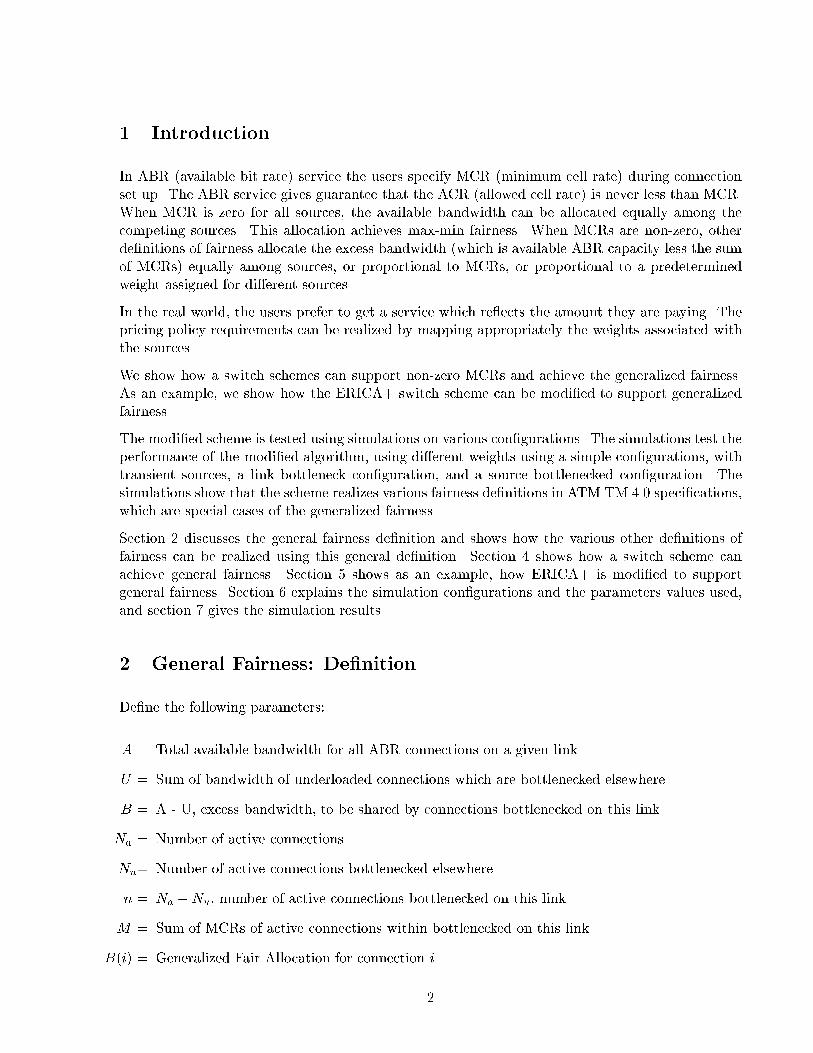
� General Fairness� De�nition

De�ne the following parameters�

A � Total available bandwidth for all ABR connections on a given link

U � Sum of bandwidth of underloaded connections which are bottlenecked elsewhere

B � A � U excess bandwidth to be shared by connections bottlenecked on this link

Na � Number of active connections

Nu� Number of active connections bottlenecked elsewhere

n � Na �Nu number of active connections bottlenecked on this link

M � Sum of MCRs of active connections within bottlenecked on this link

B�i� � Generalized Fair Allocation for connection i

�

MCR�i� � MCR of connection i

w�i� � preassigned weight associated with the connection i

The generalized fair allocation is de�ned as follows�

B�i� �MCR�i� �w�i��B �M�Pn

j��w�j�

Note that this de�nition of fairness is di�erent from the weighted allocation given as an examplefairness criterion in ATM TM �� speci�cations In the above de�nition only the excess bandwidthis allocated proportional to weights This above de�nition ensures the allocation is at least MCR

�� Mapping TM �� Fairness to Generalized Fairness

Here we show how the di�erent fairness criteria mentioned in ATM TM �� speci�cation can berealized based on the above fairness

� Max�Min� In this case MCRs are zero and the bandwidth is shared equally

B�i� � B�n

This is a special case of generalized fairness with MCR�i� � � and w�i� � c where c is aconstant

� MCR plus equal share� The excess bandwith is shared equally

B�i� �MCR�i� � �B �M��n

by assigning equal weights we achieve the above fairness

� Proportional to MCR� The allocation is proportional to its MCR

B�i� �B �MCR�i�

M�

�M �B �M�MCR�i�

M�MCR�i� �

�B �M�MCR�i�

M

By assigning w�i� � MCR�i� we can achieve the above fairness

� Relationship to Pricing�Charging Policies

Consider a very small interval T of time The charge C that a customer pays for using a networkduring this interval is a function of the number of bits W that the network transported successfully�

C � f�W�R�

�

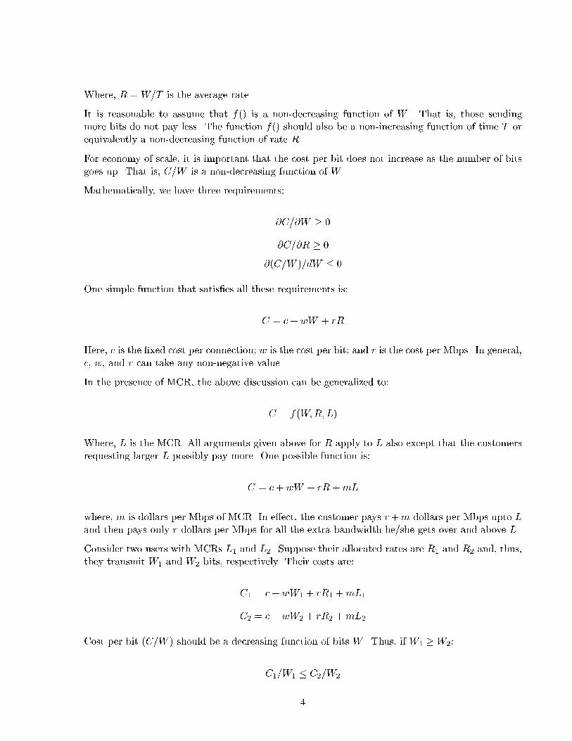
Where R �W�T is the average rate

It is reasonable to assume that f�� is a non�decreasing function of W That is those sendingmore bits do not pay less The function f�� should also be a non�increasing function of time T orequivalently a non�decreasing function of rate R

For economy of scale it is important that the cost per bit does not increase as the number of bitsgoes up That is C�W is a non�decreasing function of W

Mathematically we have three requirements�

�C��W � �

�C��R � �

��C�W ��dW � �

One simple function that satis�es all these requirements is�

C � c� wW � rR

Here c is the �xed cost per connection� w is the cost per bit� and r is the cost per Mbps In generalc w and r can take any non�negative value

In the presence of MCR the above discussion can be generalized to�

C � f�W�R�L�

Where L is the MCR All arguments given above for R apply to L also except that the customersrequesting larger L possibly pay more One possible function is�

C � c� wW � rR�mL

where m is dollars per Mbps of MCR In e�ect the customer pays r�m dollars per Mbps upto Land then pays only r dollars per Mbps for all the extra bandwidth he�she gets over and above L

Consider two users with MCRs L� and L� Suppose their allocated rates are R� and R� and thusthey transmit W� and W� bits respectively Their costs are�

C� � c� wW� � rR� �mL�

C� � c� wW� � rR� �mL�

Cost per bit �C�W � should be a decreasing function of bits W Thus if W� �W��

C��W� � C��W�

�

c�W� � w � rR��W� �mL��W� � c�W� � w � rR��W� �mL��W�

Since Ri �Wi�T we have�

c��R�T � � w � r�T �mL��R�T � � c��R�T � � w � r�T �mL��R�T �

c�R� �mL��R� � c�R� �mL��R�

�c�mL��c �mL�� R��R�

�a� L��a � L�� R��R�

Where a ��c�m� is the ratio of the �xed cost and cost per unit of MCR

Note that the allocated rates should either be proportional to a�MCR or be a non�decreasingfunction of MCR This is the policy we have chosen for this contribution

� Achieving General Fairness in Switch Algorithms

A typical ABR switch scheme calculates the excess bandwidth capacity available for best e�ortABR after reserving bandwidth for providing MCR guarantee and higher priority classes such asVBR and CBR The switch fairly divides the excess bandwidth among the connections bottleneckedat that link Therefore the ACR can be represented by the following equation

ACR�i� �MCR�i� � ExcessFairshare�i�

ExcessFairshare is the amount of bandwidth allocated over the MCR in a fair manner

In the case of general fairness the ExcessFairshare term is given by�

ExcessFairshare�i� �w�i��B �M�Pn

j��w�j�

If the network is near steady state then the above allocation enables the sources to attain thegeneralized fairness To achieve the generalized fairness the ATM TM �� speci�cation mentionsthat the value of �ACR�MCR� can be used We have to ensure the �ACR�MCR� converges tothe ExcessFairshare We use the notion of activity level to achieve the above �� A connection�sactivity level �AL�i�� is de�ned as follows

�

AL�i� � minimum��SourceRate�i��MCR�i�

ExcessFairshare�i��

SourceRate�i� is the rate at which the source is currently transmitting data Note that SourceRate�i�is the ACR�i� given as the feedback rate earlier by the switch The activity level indicates howmuch of the ExcessFairshare is actually being used by the connection The activity level attainsthe value of one when the ExcessFairshare is used by the link The weights used in the gen�eralized fairness assume that the links use their ExcessFairshare but this might not be caseBy multiplying the weights by the activity level and using these as the weights in calculating theExcessFairshare we can make sure that the rates converge to the generalized fairness allocationTherefore the ExcessFairshare share term is

ExcessFairshare�i� �w�i�AL�i��B �M�Pn

j��w�j�AL�j�

An switch algorithm can use the above ExcessFairshare term to achieve general fairness Inthe next section we show how the ERICA� switching algorithm is be modi�ed to achieve generalfairness

� Example Modi�cations to A Switch Algorithm

The ERICA� algorithm operates at each output port of a switch The switch periodically monitorsthe load on each link and determines a load factor �z� the available ABR capacity and number ofcurrently active sources or VCs �N� The measurement period is the �Averaging Interval� Thesemeasurements are used to calculate the feedback rate which is indicated in the BRM �backwardRM� cells The measurements are done in the forward direction and the feedback is given int thebackward direction The complete description of the ERICA� algorithm can be obtained from ��

The ERICA� algorithm uses the term FairShare which is the bottleneck link capacity divided bythe active number of VCs It also uses MaxAllocPrevious term which is the maximum allocationin the previous �Averaging Interval� This term is used to achieve Max�min fairness We modifythe algorithm by replacing the FairShare term by fairshare�i� and adding the MCR�i� The keyssteps in ERICA� which are modi�ed to achieve the general fairness shown below�

End of Averaging Interval�

Total ABR Capacity � Link Capacity�VBR Capacity

�nX

i��

min�SourceRate�i��MCR�i��

Target ABR Capacity � Fraction� Total ABR Capacity ��

Input Rate � ABR Input Rate�nX

i��

min�SourceRate�i��MCR�i��

z �Input Rate

Target ABR Capacity��

�

ExcessFairshare�i� ��Target ABR Capacity�w�i�AL�i�

Pnj��w�j�AL�j�

��

��

The Fraction term is dependent on the queue length Its value is one for small queue lengths anddrops sharply as queue length increases When the Fraction is less than one �� Fraction� �TotalABRCapacity is used to drain the queues ERICA� uses an hyperbolic function calculatingvalue of the Fraction

When a BRM is received�

VCShare �SourceRate�i� �MCR�i�

z��

ER � MCR�i� �Max �ExcessFairshare�i� VCShare� ��

ER in RM Cell � Min�ER in RM CellERTarget ABR Capacity� ��

The V CShare is used to achieve an unit overload When the network reaches steady state theV CShare term converges to ExcessFairshare�i� term achieving generalized fairness criterion

� Simulation Con�gurations

We use di�erent con�gurations to test the performance of the modi�ed algorithm We assume thatthe sources are greedy ie they have in�nite amount of data to send and always send data atACR In all con�gurations the data tra�c is only one way from source to destination All the linkbandwidths are �� less the SONET overhead� expect in the GFC�� con�guration

�� Three Sources

This is a simple con�guration in which three sources send to three destinations over a two switchsand a bottleneck link See �gure � Only sources send data This con�guration is used to demon�strate that the modi�ed switchs algorithm can achieve the general fairness for the various set ofweight assignments

Destination 2

Source 1

Source 2 Switch 1 Switch 2

Bottleneck Link

Destination 1

Source 3 Destination 3

Figure �� N Sources � N Destinations Con�guration

�

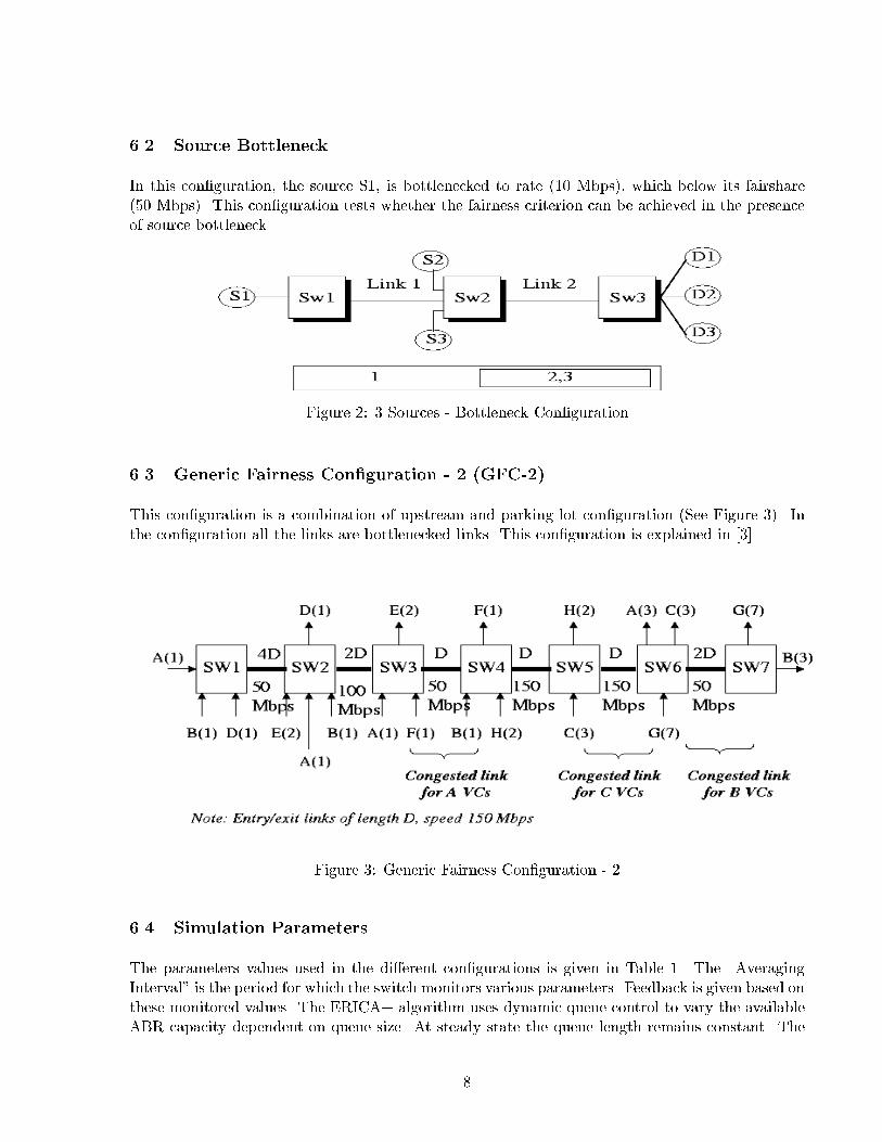
�� Source Bottleneck

In this con�guration the source S� is bottlenecked to rate �� Mbps� which below its fairshare�� Mbps� This con�guration tests whether the fairness criterion can be achieved in the presenceof source bottleneck

��

Figure �� Sources � Bottleneck Con�guration

�� Generic Fairness Con�guration � � GFC��

This con�guration is a combination of upstream and parking lot con�guration �See Figure �� Inthe con�guration all the links are bottlenecked links This con�guration is explained in ��

��

Figure �� Generic Fairness Con�guration � �

�� Simulation Parameters

The parameters values used in the di�erent con�gurations is given in Table � The �AveragingInterval� is the period for which the switch monitors various parameters Feedback is given based onthese monitored values The ERICA� algorithm uses dynamic queue control to vary the availableABR capacity dependent on queue size At steady state the queue length remains constant The

�

Table �� Simulation Parameter Values

Con�guration Link Averaging TargetName Distance interval Delay

Three Sources �� Km � ms �� msSource Bottleneck �� Km � ms �� ms

GFC�� Km �� ms �� ms

Table �� Three sources con�guration simulation results

ExpectedCase Src mcr a weight fair Actual

Number Num function share share

� � � � � ��

� � ��

� � ��

�Target Delay� parameter speci�es the desired delay due to this constant queue length at steadystate

Simulation Results

In this section we give the simulation results for the di�erent con�gurations

�� Three Sources

Simulations using a number of weight functions were done using the simple three sources con�gu�ration to demonstrate that general fairness is achieved in all these cases The ICRs of the sourceswere set to the �� in all the simulations The results of these cases are given in Table � TheFigure � shows the ACRs of the three sources and the queue length to bottleneck link at switch��

The following can be observed from the Table �

� Case �� a � � MCRs � � All weights are equal so the allocation �� foreach connection This is allocation is the same as max�min fair allocation

�

Table �� Three sources transient con�guration simulation results

Expected Actual Expected ActualCase Src mcr a weight fairshare �non�trans� fairshare �trans�

Number Num function �non�trans� share �trans� share

� � � � � ��

� � ��

� � ��

� Case �� a �� MCRs �� The left over capacity �� is dividedequally among the three sources So the allocation is ��

� Case �� a � � MCRs �� Hence the weight function is � � MCR The left over capacity�� Mbps is divided proportional to �� Hence the allocation is ��

�� Three Sources� Transient

In these simulations the same simple three source con�guration is used The source � and source� transmit data throughout the simulation period The source S� is a transient source whichstarts transmitting at �� ms and stops at �� ms The total simulation time is �� ms The sameparameters values from the case�s � � and � of the previous sections were used in these simulationsThe results of these simulations are given in Table � The �non�trans� columns give the allocationwhen source � is not present ie between �ms to ��ms and between ��ms to �� ms The�trans� columns give allocation when the transient source � is present ie between �� ms to ��ms

The graphs for these three simulations are shown in �gure � The graphs show the ACRs of the threesources and the bottleneck link utilization It can be seen both from the Table � and the graphsthat the switch algorithm does converge to the general fairness allocation even in the presence oftransient sources Note the link utilization is high throughout the simulation The width of dipin the utilization graph when the transient sources goes away indicates the reponsiveness of thealgorithm This shows that the algorithm is tolerant of transient sources and responds quickly tochanging demands

��

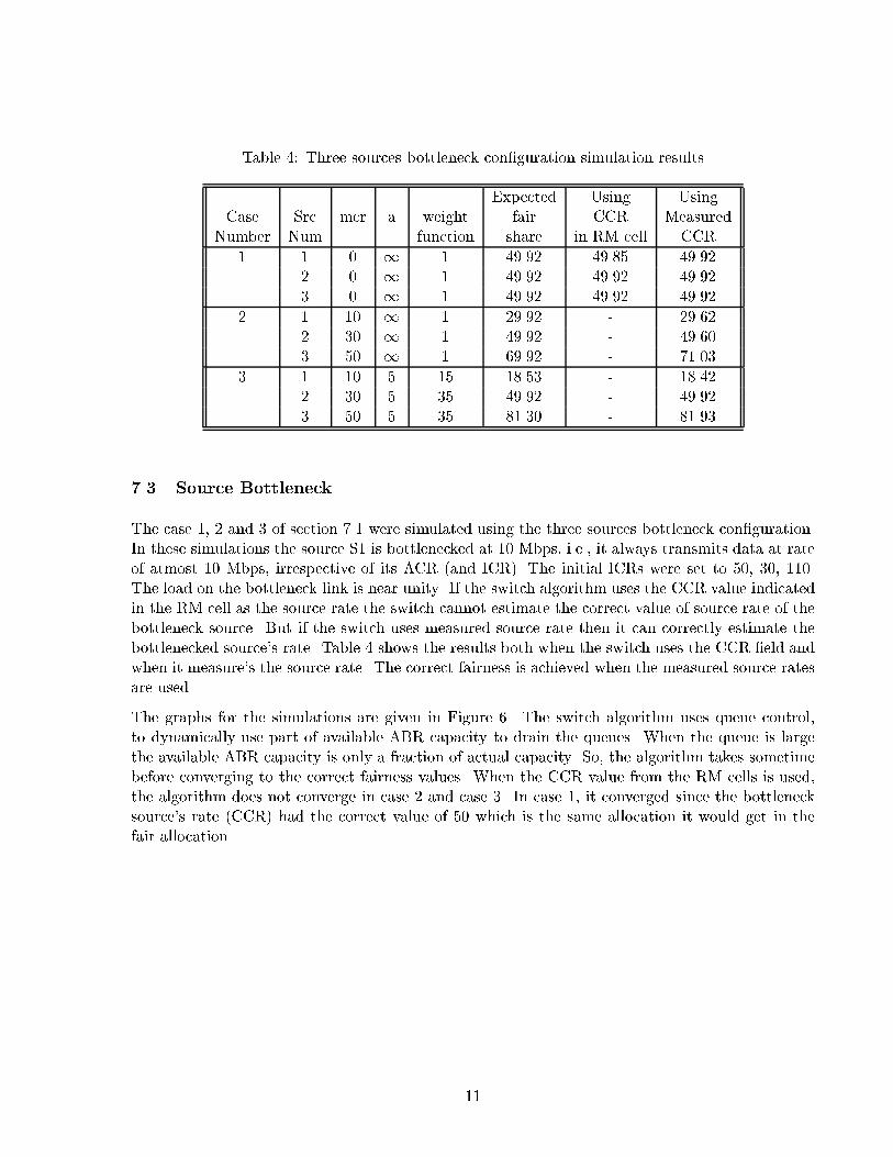
Table �� Three sources bottleneck con�guration simulation results

Expected Using UsingCase Src mcr a weight fair CCR Measured

Number Num function share in RM cell CCR

� � � � � ��

� � ��

� � ��

�� Source Bottleneck

The case � � and � of section �� were simulated using the three sources bottleneck con�gurationIn these simulations the source S� is bottlenecked at �� Mbps ie it always transmits data at rateof atmost �� Mbps irrespective of its ACR �and ICR� The initial ICRs were set to �� The load on the bottleneck link is near unity If the switch algorithm uses the CCR value indicatedin the RM cell as the source rate the switch cannot estimate the correct value of source rate of thebottleneck source But if the switch uses measured source rate then it can correctly estimate thebottlenecked source�s rate Table � shows the results both when the switch uses the CCR �eld andwhen it measure�s the source rate The correct fairness is achieved when the measured source ratesare used

The graphs for the simulations are given in Figure � The switch algorithm uses queue controlto dynamically use part of available ABR capacity to drain the queues When the queue is largethe available ABR capacity is only a fraction of actual capacity So the algorithm takes sometimebefore converging to the correct fairness values When the CCR value from the RM cells is usedthe algorithm does not converge in case � and case � In case � it converged since the bottlenecksource�s rate �CCR� had the correct value of �� which is the same allocation it would get in thefair allocation

��

ICR:50.00 10.00 40.00 10.00 55.00 10.00 / XRM:253.00 253.00 253.00 253.00 253.00 253.00 / Graph: 0

abr_3.snapfile/case=case25_1/option=14403/optionb=295/dist=1000/

stoptime=600000/exp_avg_N=0.9/t0v=1500/f_r=5000/ / Date:01/26/98�

0

20

40

60

80

100

120

140

160

0 100 200 300 400 500 600

AC

R (

Mb/

s)

Time in milliseconds

3 Sources: ACR for ABR sources

ACR of abr[1] ACR of abr[2] ACR of abr[3]

�a�

ICR:50.00 10.00 40.00 10.00 55.00 10.00 / XRM:253.00 253.00 253.00 253.00 253.00 253.00 / Graph: 0



0

50

100

150

200

250

300

350

400

0 100 200 300 400 500 600 700

Que

ue le

ngth

(ce

lls)


3 Sources : Bottleneck Queues

ABR Queue

�b�

ICR:50.00 10.00 40.00 10.00 55.00 10.00 / XRM:253.00 253.00 253.00 253.00 253.00 253.00 / Graph: 0



0

20

40

60

80

100

120

140

160

0 100 200 300 400 500 600

AC

R (

Mb/

s)




�c�

ICR:50.00 10.00 40.00 10.00 55.00 10.00 / XRM:253.00 253.00 253.00 253.00 253.00 253.00 / Graph: 0



0

100

200

300

400

500

600

700

800

0 100 200 300 400 500 600 700

Que

ue le

ngth

(ce

lls)



ABR Queue

�d�

ICR:50.00 10.00 40.00 10.00 55.00 10.00 / XRM:253.00 253.00 253.00 253.00 253.00 253.00 / Graph: 0



0

20

40

60

80

100

120

140

160

0 100 200 300 400 500 600

AC

R (

Mb/

s)




�e�

ICR:50.00 10.00 40.00 10.00 55.00 10.00 / XRM:253.00 253.00 253.00 253.00 253.00 253.00 / Graph: 0



0

200

400

600

800

1000

1200

0 100 200 300 400 500 600

Que

ue le

ngth

(ce

lls)



ABR Queue

�f�

Figure �� Three Sources� ACR graphs and Queue length of bottleneck link

��

ICR:50.00 10.00 40.00 10.00 55.00 10.00 / XRM:253.00 253.00 253.00 253.00 253.00 253.00 / Graph: 0

abrtrans_3.snapfile/case=trans_1/option=14531/optionb=295/dist=1000

/stoptime=1200000/exp_avg_N=0.9/f_r=5000/t0v=1500/ / Date:01/26/98�

0

20

40

60

80

100

120

140

160

0 200 400 600 800 1000 1200

AC

R (

Mb/

s)




�a�

ICR:50.00 10.00 40.00 10.00 55.00 10.00 / XRM:253.00 253.00 253.00 253.00 253.00 253.00 / Graph: 0



0

20

40

60

80

100

0 200 400 600 800 1000 1200

Lin

k U

tiliz

atio

n M

b/s


3 Sources : Bottleneck Link Utilization

Link utilization to sw[1]

�b�

ICR:50.00 10.00 40.00 10.00 55.00 10.00 / XRM:253.00 253.00 253.00 253.00 253.00 253.00 / Graph: 0



0

20

40

60

80

100

120

140

160

0 200 400 600 800 1000 1200

AC

R (

Mb/

s)




�c�

ICR:50.00 10.00 40.00 10.00 55.00 10.00 / XRM:253.00 253.00 253.00 253.00 253.00 253.00 / Graph: 0



0

20

40

60

80

100

0 200 400 600 800 1000 1200

Lin

k U

tiliz

atio

n M

b/s




�d�

ICR:50.00 10.00 40.00 10.00 55.00 10.00 / XRM:253.00 253.00 253.00 253.00 253.00 253.00 / Graph: 0



0

20

40

60

80

100

120

140

160

0 200 400 600 800 1000 1200

AC

R (

Mb/

s)




�e�

ICR:50.00 10.00 40.00 10.00 55.00 10.00 / XRM:253.00 253.00 253.00 253.00 253.00 253.00 / Graph: 0



0

20

40

60

80

100

0 200 400 600 800 1000 1200

Lin

k U

tiliz

atio

n M

b/s




�f�

Figure �� Three Sources �Transient� � ACR and Utilization graphs

��

ICR:50.00 25.00 30.00 25.00 110.00 25.00 / XRM:253.00 253.00 253.00 253.00 253.00 253.00 / Graph: 0

btlnk.snapfile/option=14403/optionb=110/stoptime=800000/exp_avg_N=0.9/icr=25.0/icr1=50.0/icr2=30.0/icr3=110.0/xdf=0.0/tdf=0.0

/t0v=1500/air=1.0/sw_int=100/t_threshold=400000/maxsrcrate=10.0/mib=20000/mib=20000/wandist=1000/case=case_1/ / Date:01/26/98�

0

20

40

60

80

100

120

140

160

180

0 100 200 300 400 500 600 700 800

AC

Rs


WAN Bottlenecked: ACRs

ACR for S1 ACR for S2 ACR for S3

�a�

ICR:50.00 25.00 30.00 25.00 110.00 25.00 / XRM:253.00 253.00 253.00 253.00 253.00 253.00 / Graph: 0

btlnk.snapfile/option=14531/optionb=110/stoptime=800000/exp_avg_N=0.9/icr=25.0/icr1=50.0/icr2=30.0/icr3=110.0/xdf=0.0/tdf=0.0/t0

v=1500/air=1.0/sw_int=100/t_threshold=400000/maxsrcrate=10.0/mib=20000/mib=20000/wandist=1000/case=case_pervc_1/ / Date:01/26/98�

0

20

40

60

80

100

120

140

160

180

0 100 200 300 400 500 600 700 800

AC

Rs




�b�

ICR:50.00 25.00 30.00 25.00 110.00 25.00 / XRM:253.00 253.00 253.00 253.00 253.00 253.00 / Graph: 0



0

20

40

60

80

100

120

140

160

180

0 100 200 300 400 500 600 700 800

AC

Rs




�c�

ICR:50.00 25.00 30.00 25.00 110.00 25.00 / XRM:253.00 253.00 253.00 253.00 253.00 253.00 / Graph: 0



0

20

40

60

80

100

120

140

160

180

0 100 200 300 400 500 600 700 800

AC

Rs




�d�

ICR:50.00 25.00 30.00 25.00 110.00 25.00 / XRM:253.00 253.00 253.00 253.00 253.00 253.00 / Graph: 0



0

20

40

60

80

100

120

140

160

180

0 100 200 300 400 500 600 700 800

AC

Rs




�e�

ICR:50.00 25.00 30.00 25.00 110.00 25.00 / XRM:253.00 253.00 253.00 253.00 253.00 253.00 / Graph: 0



0

20

40

60

80

100

120

140

160

180

0 100 200 300 400 500 600 700 800

AC

Rs




�f�

Figure �� Three Sources Bottleneck� ACR graphs �with and without measuring Source Rate�

��

0

20

40

60

80

100

120

140

160

180

0 500 1000 1500 2000 2500 3000

AC

Rs


GFC-2: ACRs

A_SW1 B_SW1 C_SW5 D_SW1 E_SW2 F_SW3 G_SW6 H_SW4

�a�

0

5000

10000

15000

20000

25000

30000

0 500 1000 1500 2000 2500 3000

Que

ue L

engt

h (c

ells

)


GFC-2: Queue Lengths

Queue Length 1 Queue Length 2 Queue Length 3 Queue Length 4 Queue Length 5 Queue Length 6

�b�

Figure �� GFC�� con�guration� ACRs of A through H VCs and Queue lengths at bottlenecks links

Table �� GFC�� con�guration� simulation results

Case VC Expected ActualNumber type allocation Allocation

� A �� B � ��

�a � �� C �� D ��

�all MCRs E �� are zero� F �� same as G � ��max�min� H ��

�� Link Bottleneck� GFC��

In this con�guration each link is a bottleneck link The Figure � �a� shows the ACR graphs foreach type of VCs Figure � �b� shows the queue length of all the bottleneck links �links betweenthe switches� From the Figure and Table � it can be seen that the VCs converge to their expectedfairshare This shows that the algorithm works in the presence of link bottlenecks

Conclusion

In this contribution we have given a general de�nition of fairness which inherently provides MCRguarantee and divides the excess bandwidth proportional to predetermined weights Di�erentfairness criterion such as max�min fairness MCR plus equal share proportional MCR can berealized as special cases of this general fairness We showed how to realize a typical pricing policyby appropriate weight function The general fairness can be achieved by using the ExcessFairshare

��

term in the switch algorithms The weights are multiplied by the activity level when calculatingthe ExcessFairshare to re�ect the actual usage of the source

We have shown how ERICA� switch algorithm can be modi�ed achieve this general fairness Themodi�ed algorithm has been tested under di�erent con�guration using persisent sources The sim�ulations results show that the modi�ed algorithm achieves the general fairness in all con�gurationsIn source bottlenecked con�guration the value of the CCR from the RM cell maybe incorrectHence it is necessary to used the measured source rate in the presence of source bottlenecks

References

�� Shirish S Sathaye ATM Forum Tra�c Management Speci�cation Version �� April ��

�� Raj Jain Shivkumar Kalyanaraman Rohit Goyal Sonia Fahmy and Ram Viswanathan ER�ICA switch algorithm� A complete description ATM Forum�� August ��

�� Robert J Simcoe Test con�gurations for fairness and other tests ATM Forum�� July��

�� Sonia Fahmy Raj Jain Shivkumar Kalyanaraman Rohit Goyal and Bobby Vandalore Deter�mining the number of active ABR sources in switch algorithms ATM Forum�� February��

��

Documents

A Definition of Generalized Fairness and its Support in ...jain/atmf/ftp/atm98-0151.pdf · transien t sources a link b ottlenec k conguration and source ed conguration The sim ulations