A Deep Generative Model for Non-intrusive Identification

1949-3053 (c) 2020 IEEE. Personal use is permitted, but republication/redistribution requires IEEE permission. See http://www.ieee.org/publications_standards/publications/rights/index.html for more information.

This article has been accepted for publication in a future issue of this journal, but has not been fully edited. Content may change prior to final publication. Citation information: DOI 10.1109/TSG.2020.2998080, IEEETransactions on Smart Grid

1

A Deep Generative Model for Non-intrusiveIdentification of EV Charging Profiles

Shengyi Wang, Student Member, IEEE, Liang Du, Senior Member, IEEE, Jin Ye, Senior Member, IEEE,

Dongbo Zhao, Senior Member, IEEE

Abstract—The proliferation of electric vehicles (EVs) bringsenvironmental benefits and technical challenges to power grids.An identification algorithm which can accurately extract indi-vidual EV charging profiles out of widely available smart metermeasurements has attracted great interests. This paper proposesa non-intrusive identification framework for EV charging profileextraction, which is driven by deep generative models (DGM).First, the proposed DGM is designed as a representation layerembedded into the Markov process and used to model the jointprobability distribution of available time-series data. A novelcontribution is to approximate posterior distributions by neuralnetworks whose parameters are obtained by variational inferenceand supervised learning. Second, the EV charging status isinferred from the DGM via dynamic programming. Lastly, thedesired EV charging profile can be reconstructed by the ratedpower of EV models and inferred status. Compared with thebenchmark Hidden Markov Models, the proposed framework canbetter handle noise in data with less computational complexityand better overall accuracy performances with smaller recall.The proposed framework is validated by numerical experimentson the Pecan Street dataset.

Index Terms—electric vehicles charging, energy disaggrega-tion, load modeling, deep learning, statistical inference

NOMENCLATURE

⇡ prior probability vector of initial EV charging status⇡i probability of initial EV charging status being i

⇡⇤i estimated ⇡i

1ij indicator functionA probability transition matrixAij probability of EV charging status transits from i to j

A⇤ij estimated Aij

N number of labeled dataNb minibatch sizeP EV charging profilep(yt) probability distribution of EV charging status at tPt charging power of an EV charging profile P at tx aggregate power consumption profile by AMIs

Manuscript received September 4, 2019; revised January 13, 2020 and April9, 2020; accepted May 24, 2020. Date of publication XXXXXX, 2020; date ofcurrent version XXXXXXX, 2020. This work was supported in part by OakRidge Associated Universities (ORAU) under Ralph E. Powe Junior FacultyEnhancement Award (L. Du). The work of J. Ye was supported by the NationalScience Foundation under Grant ECCS-1946057. (Corresponding author: L.Du.)

S. Wang and L. Du are with the Department of Electrical and Com-puter Engineering, Temple University, Philadelphia, PA 19122 USA e-mail:{shengyi.wang, ldu}@temple.edu.

J. Ye is with the School of Electrical and Computer Engineering, Universityof Georgia, Athens, GA 30602 USA e-mail: [email protected].

D. Zhao is with Argonne National Laboratory, Lemont, IL 60439 USAe-mail: [email protected].

xt value of x at time t

yt EV charging status at ty(n)t EV charging status of the n-th labeled data at tz layer to represent the aggregate power consumption.

I. INTRODUCTION

The worldwide electricity demand profile is experiencinga paradigm shift with increasing penetration of electrifiedtransportation. In the U.S., it is expected that transportationelectrification will drive domestic electricity demand risethrough 2050 [1], by when over 2.3 million new light-dutyelectric vehicles (EVs) will be sold annually [2]. Across theglobe, many major economies have announced their intentionsto end the sale of internal combustion engine vehicles [3]within several decades. The impact of high volume of EVson power grids has been extensively studied in literature [4].In general, EVs have been considered as active loads whichcould provide flexibility in terms of grid services [5] throughvehicle-to-grid (V2G) modes [6] or transactive controls [7].

In the literature, aggregated EV charging demands are mod-eled as a stochastic part of the overall load model. However,the uncertainty in individual EV charging profiles (i.e., startcharging time, initial state-of-charge (SOC), charging power,and charging duration) [8] and traffic conditions [9] makes itdifficult to accurately derive real-time EV charging demandmodels under various scenarios. Therefore, probabilistic dis-tributions are typically assumed. In [10] and [11], the chargingstart time is represented by the normal distribution. Similar,a truncated normal distribution is suggested to represent thearriving time and parking time at commercial buildings [12]for EV charging duration. Furthermore, in [13], EV chargingduration is assumed to be exponentially distributed. Moreover,the initial SOC is modeled as a random variable under log-normal distribution [8]. However, it is questionable whetherthese assumptions from locational models can be used in otherregions. For example, charging start times in rural residential,urban residential, and commercial districts at different seasonsare unlikely to be the same. Therefore, in recent years, pilotprojects have been carried out globally to collect and analyzeEV charging profiles in the Netherlands [14], U.K. [15],Australia [16], and California [17].

However, most of the historical data is only small-scaleand sampled at commercial charging stations. For residentialapplications, it is costly to (intrusively) install additionalsampling devices into existing residential EV chargers and(more importantly) unrealistic to sample and communicate



2

EV charging information to system operators, another recentresearch effort [18]–[22] focuses on utilizing widely-availablesmart meter data to non-intrusively, locally, and reliably esti-mate EV charging profiles in real-time to preserve privacy andavoid unnecessary investment in additional infrastructure.

To conclude above discussions, it is of great interests forsystem operators and planners to extract EV charging profilesfrom smart meter data in a non-intrusive manner such that1) unrealistic and uncertain assumptions (as pointed out inthe above discussions) can be alleviated; and 2) EV chargingprofiles can be accurately extracted in real-time to support bothshort-term system operations and long-term planning.

To our best knowledge, reference [19] is probably the firstto adopt non-intrusive load monitoring (NILM) and applybenchmark algorithms such as the Hidden Markov Models(HMMs) [23] to detect events and disaggregate EV chargingprofiles from low-frequency smart meter readings. Reference[20] presents an unsupervised algorithm to extract EV chargingloads non-intrusively from the smart meter data using indepen-dent component analysis. Reference [21] aims at identifyingEV models to determine charging power. Finally, reference[22] proposes a training-free non-intrusive algorithm basedon bounding-box fitting and load signatures. To summarize,HMMs are probably the most popular identification models,which are relatively easy to train but require detailed prior in-formation of all appliances in the aggregated power consump-tion profiles (and thus cannot tackle unknown appliances).Moreover, computational complexity of an exact inference inHMMs grows exponentially with the sequence lengths andthe number of appliances. Therefore, it is desired to design analgorithm to mitigate the aforementioned issues.

This paper retains the Markov property in HMMs but onlyutilizes one Markov chain to involve only the aggregatedand partial EV charging data points as known information.Without involving other appliances’ power consumption data,the computational complexity of an exact inference is greatlyreduced. Specifically, this paper proposes a deep generativemodel (DGM)-driven inference framework for non-intrusive,real-time identification of EV charging profiles. Firstly, thejoint probability distribution for available smart meter data(which can actually be considered as time series) is modeledby deep generative models (DGMs). A novel contributionby this paper is to approximate posterior distributions byneural networks whose parameters are obtained by variationalinference and supervised learning. Secondly, the EV chargingstatus is inferred from DGMs via dynamic programming.Finally, the target EV charging profile can be reconstructedaccording to the rated power of EV models and inferred status.

The main contributions of this paper are listed as follows.

• Compared to the existing literature in which most worksneed to manually define features, the proposed DGMwith convolutional neural layers can automatically ex-tract features and represent highly nonlinear features ofaggregated power consumption profile with less weights.

• Compared to the existing literature in which assumptionson prior knowledge are typically made, the proposedframework makes full use of smart meter data to extract

Classification

Reconstruction

Identification

Energy Flow

Information Flow

Smart Meter

Charger

(a)

(b)

(c)

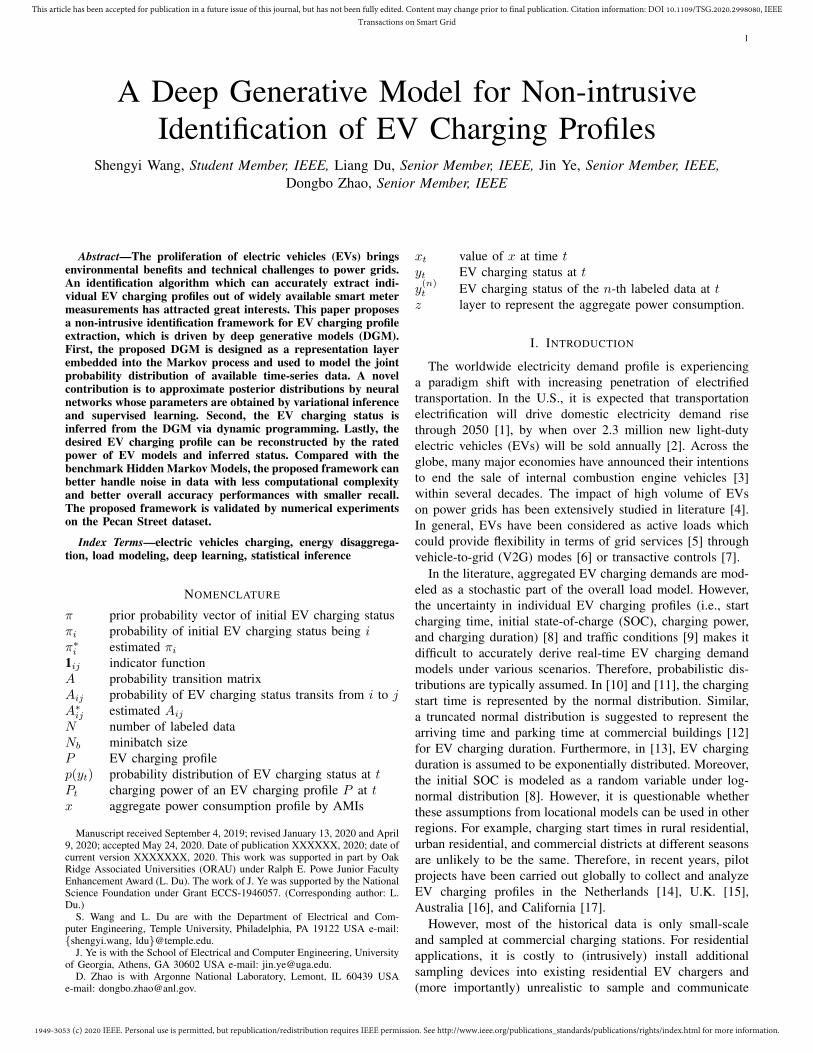
Fig. 1. Overview of EV charging profile identification. (a): a sampleaggregated power consumption profile; (b): its corresponding EV chargingstatus (charging started at ts and ended at te); and (c) its corresponding EVcharging profile.

EV charging profiles without any need of prior knowledgein other appliances being used at the same time as EVs.

• Two different schemes with both transfer and non-transferlearning settings have been studied, and results showthat the proposed framework possesses good robustnessagainst noise and error in data as well as generalizationcapability to unseen data.

The remainder of this paper is organized as follows. SectionII defines the EV charging profile identification problemconsidered in this paper and then formulates it with in thearchitecture of NILM. Next, Section III reviews the frameworkof HMM, which will be used as a benchmark algorithm.Furthermore, Section IV proposes a DGM to model the jointprobability distribution of the available aggregated consump-tion data, of which parameters are obtained by variationalinference and supervised learning. Section V utilizes dynamicprogramming to perform exact inference of the DGM for theEV charging status. Moreover, Section VI discusses numericalvalidation setup and results. Finally, Section VII presentsconclusions and future work.

II. PROBLEM FORMULATION

The EV charging profile identification problem consideredin this paper is presented in Fig. 1, in which a sampleaggregated power consumption profile is shown in Fig. 1(a),with its corresponding EV charging profile shown in Fig. 1(c).Furthermore, Fig. 1(b) shows the corresponding EV chargingstatus (charging started at time ts and ended at time te).

A. Definitions

Given an aggregated power consumption profile x =(x1, . . . , xT ), i.e., a timed sequence of a total of T powerconsumption data points, determine its corresponding EVcharging profile P (or P (x) if the source power consumptionprofile x is relevant). Note that the power consumption profileis called aggregated as most smart meters measure the powerconsumption of the whole household and thus include allloads (i.e., aggregated). An EV charging profile is thus atimed sequence (of the same length T ) of EV charging powerconsumption data points. In other words, the value Pt of P attime step t denotes the amount of power by EV charging.



3

Moreover, at time step t, the charging status yt of an EVis binary, i.e., either ON (i.e., yt = 1 if Pt is greater thana pre-defined threshold Pth) or OFF (yt = 0 otherwise).Furthermore, the probability of an EV at its yt is denotedby p(yt). When yt = 1, p(yt = 1) = 1 and p(yt = 0) = 0.When yt = 0, p(yt = 1) = 0 and p(yt = 0) = 1.

B. EV Charging Profile Identification as NILM

The objective of the EV charging profile identificationproblem considered in this paper is to determine EV chargingprofile P given aggregated power consumption profile x.Therefore, the scope of this work falls within the framework ofa NILM problem. Most techniques used for NILM problemsin the literature consist of two sub-tasks: 1) classification and2) reconstruction. The former task aims at classifying the loadoperation status into known categories, and the latter task isto reconstruct load consumption profiles using classificationresults. For example, if the first task returns that the chargingstatus of a certain model of EV at time step t is classified tobe ON (i.e., yt = 1) with rated power consumption around 6.7kW (i.e., Pt = 6.7), then the latter task would focus on re-constructing its corresponding EV charging profile. Therefore,this paper follows [21], [24] to assume that EV charging powerlevel and corresponding models can be identified separatelyand mainly focuses on EV charging status classification andconverts the EV charging profile identification problem into abinary EV charging status classification task.

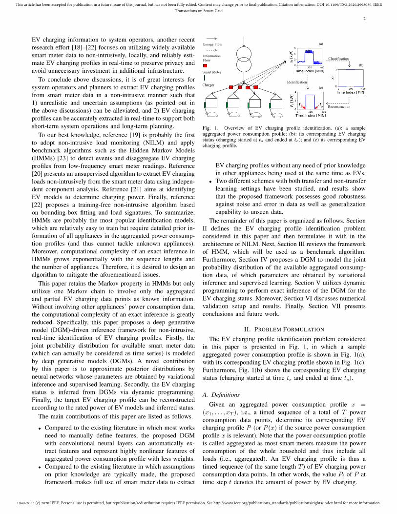
Therefore, the EV charging profile identification problemthis paper aims to solve can be formulated as follows: givenan aggregated power consumption profile x = (x1, . . . , xT ),determine yt of an EV at each time step t = 1, . . . , T . Thegeneral procedure of how the proposed EV charging profileidentification problem is studied in this paper is presented inFig. 2. First of all, each generative process for time-seriesdata is modeled by a joint probability distribution in Step 1.Secondly, each component (e.g., evidence and transition prob-abilities) in the joint distribution from Step 1 is approximatedby a common parametric density function in Step 2. Thirdly,parameters of the density function (in the joint distribution)from Step 2 are learned by maximum likelihood estimationin Step 3. Finally, the above-defined identification problem isconverted to a Bayesian inference process by the proposedDGM in Step 4. The above steps are further specified inSections IV and V.

III. BENCHMARK ALGORITHM: HMMS

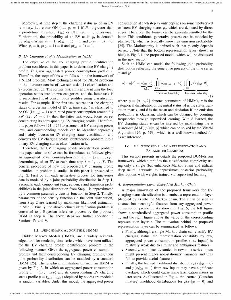
Hidden Markov Models (HMMs) are a widely acknowl-edged tool for modeling time series, which have been utilizedfor the EV charging profile identification problem in thefollowing manner. Given the aggregated power consumptionprofiles and their corresponding EV charging profiles, theirjoint probability distribution can be modeled by a standardHMM [25]. The graphical illustration of such an HMM isgiven by Fig. 3, in which an aggregated power consumptionprofile x = (x1, ..., xT ) and its corresponding EV chargingstatus profile y = (y1, ..., yT ) (depicted by nodes) are modeledas random variables. Under this model, the aggregated power

consumption at each step xt only depends on some unobservedor latent EV charging status yt, which are depicted by directedges. Therefore, the former can be generated/emitted by thelatter. This conditional generative process can be modeled byp(xt|yt, ✓), which is typically known as emission probability[25]. The Markovianity is defined such that yt only dependson yt�1. Note that the bottom representation layer (shown inblue) in Fig. 3 is the proposed model, which will be discussedin the next section.

Such an HMM can model the following joint probabilitydistribution reflecting the generative process of the time seriesx and y:

p(x, y|�) = p(y1|⇡)| {z }Prior

⇥ TY

t=2

p(yt|yt�1, A)⇤

| {z }Transition Probability

⇥ TY

t=1

p(xt|yt, ✓)⇤

| {z }Emission Probability

(1)where � = {⇡, A, ✓} denotes parameters of HMMs, ⇡ is thecategorical distribution of the initial status, A is the status tran-sition matrix, and ✓ is the mean and deviation if the emissionprobability is Gaussian, which can be obtained by countingfrequencies through supervised learning. With � learned, theEV charging status y can be inferred by maximizing the a

posteriori (MAP) p(y|x,�) which can be solved by the ViterbiAlgorithm [26, p. 629], which is a well-known method forexact inference.

IV. THE PROPOSED DGM: REPRESENTATION ANDPARAMETER LEARNING

This section presents in details the proposed DGM-drivenframework, which simplifies the classification complexity us-ing only a single (but enhanced) Markov chain and utilizesdeep neural networks to approximate posterior probabilitydistributions with weights trained via supervised learning.

A. Representation Layer Embedded Markov Chain

A major innovation of the proposed framework for EVcharging status classification is to embed a representation layer(denoted by z) into the Markov chain. The z can be seen asabstract but meaningful features from any aggregated powerconsumption profile x. As shown in Fig. 5, the left figureshows a standardized aggregated power consumption profilex, and the right figure shows the value of the correspondingrepresentation layer z. The motivation behind the proposedrepresentation layer can be summarized as follows.

• Firstly, although a single Markov chain can classify EVcharging status, the representation capability by raw,aggregated power consumption profiles (i.e., inputs) isrelatively weak due to similar and ambiguous features;

• Secondly, nonlinear dynamics in raw time-series inputsmight present higher non-stationary variances and thusfail to provide useful features;

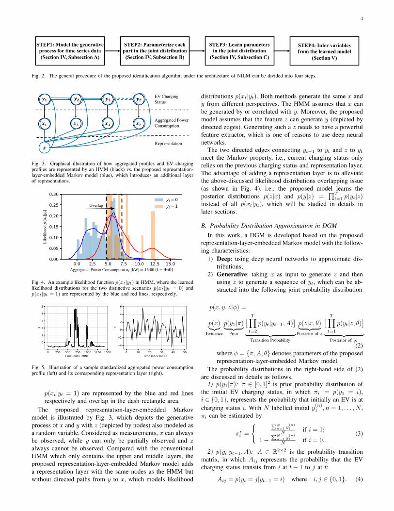
• Finally, the learned likelihood distributions p(xt|yt = 0)and p(xt|yt = 1) from raw inputs may have significantoverlaps, which could cause mis-classification issues inlater steps. As illustrated in Fig. 4, the learned (Gaussianmixture) likelihood distributions for p(xt|yt = 0) and

4

STEP1: Model the generative process for time series data(Section IV, Subsection A)

STEP2: Parameterize each part in the joint distribution(Section IV, Subsection B)

STEP3: Learn parameters in the joint distribution

(Section IV, Subsection C)

STEP4: Infer variables from the learned model

(Section V)

Fig. 2. The general procedure of the proposed identification algorithm under the architecture of NILM can be divided into four steps.

!" !# !$ !%

&" &# &$ &%

EV Charging Status

Aggregated Power Consumption

'Representation

Fig. 3. Graphical illustration of how aggregated profiles and EV chargingprofiles are represented by an HMM (black) vs. the proposed representation-layer-embedded Markov model (blue), which introduces an additional layerof representations.

Overlap

Fig. 4. An example likelihood function p(xt|yt) in HMM, where the learnedlikelihood distributions for the two distinctive scenarios p(xt|yt = 0) andp(xt|yt = 1) are represented by the blue and red lines, respectively.

Fig. 5. Illustration of a sample standardized aggregated power consumptionprofile (left) and its corresponding representation layer (right).

p(xt|yt = 1) are represented by the blue and red linesrespectively and overlap in the dash rectangle area.

The proposed representation-layer-embedded Markovmodel is illustrated by Fig. 3, which depicts the generativeprocess of x and y with z (depicted by nodes) also modeled asa random variable. Considered as measurements, x can alwaysbe observed, while y can only be partially observed and z

always cannot be observed. Compared with the conventionalHMM which only contains the upper and middle layers, theproposed representation-layer-embedded Markov model addsa representation layer with the same nodes as the HMM butwithout directed paths from y to x, which models likelihood

distributions p(xt|yt). Both methods generate the same x andy from different perspectives. The HMM assumes that x canbe generated by or correlated with y. Moreover, the proposedmodel assumes that the feature z can generate y (depicted bydirected edges). Generating such a z needs to have a powerfulfeature extractor, which is one of reasons to use deep neuralnetworks.

The two directed edges connecting yt�1 to yt and z to yt

meet the Markov property, i.e., current charging status onlyrelies on the previous charging status and representation layer.The advantage of adding a representation layer is to alleviatethe above-discussed likelihood distributions overlapping issue(as shown in Fig. 4), i.e., the proposed model learns theposterior distributions p(z|x) and p(y|z) =

QTt=1 p(yt|z)

instead of all p(xt|yt), which will be studied in details inlater sections.

B. Probability Distribution Approximation in DGM

In this work, a DGM is developed based on the proposedrepresentation-layer-embedded Markov model with the follow-ing characteristics:

1) Deep: using deep neural networks to approximate dis-tributions;

2) Generative: taking x as input to generate z and thenusing z to generate a sequence of yt, which can be ab-stracted into the following joint probability distribution

p(x, y, z|�) =

p(x)|{z}Evidence

p(y1|⇡)| {z }Prior

⇥ TY

t=2

p(yt|yt�1, A)⇤

| {z }Transition Probability

p(z|x, ✓)| {z }Posterior of z

⇥ TY

t=1

p(yt|z, ✓)⇤

| {z }Posterior of yt

(2)where � = {⇡, A, ✓} denotes parameters of the proposedrepresentation-layer-embedded Markov model.

The probability distributions in the right-hand side of (2)are discussed in details as follows.

1) p(y1|⇡): ⇡ 2 [0, 1]2 is prior probability distribution ofthe initial EV charging status, in which ⇡i := p(y1 = i),i 2 {0, 1}, represents the probability that initially an EV is atcharging status i. With N labelled initial y(n)1 , n = 1, . . . , N ,⇡i can be estimated by

⇡⇤i =

( PNn=1 y(n)

1N if i = 1;

1�PN

n=1 y(n)1

N if i = 0.(3)

2) p(yt|yt�1, A): A 2 R2⇥2 is the probability transitionmatrix, in which Aij represents the probability that the EVcharging status transits from i at t� 1 to j at t:

Aij = p(yt = j|yt�1 = i) where i, j 2 {0, 1}. (4)



5

With N labelled y(n)t , n = 1, . . . , N , Aij can be estimated by

A⇤ij =

PNn=1

PTt=2 1ij(y

(n)t = j|y(n)t�1 = i)

N(T � 1), (5)

where 1ij(yt = ·|yt�1 = ·) is an indicator function whoseoutput is 1 if and only if y(n)t = j and y

(n)t�1 = i.

3) p(z|x, ✓) and p(yt|z, ✓): Recall that an abstract butmeaningful feature, z is always unobservable. Therefore, thetrue posterior distribution of z given x is unknown. Thispaper follows [27], [28] to assume that p(z|x, ✓) takes on anapproximate Gaussian form, i.e., a multivariate Gaussian witha diagonal covariance, given as

log p(z|x, ✓) = logN(z|µz(x),�2z(x)I) (6)

where µz(x) and �z(x) are the mean and standard deviation ofz, respectively. Because yt is a binary variable, it is assumedthat yt follows a Bernoulli distribution

log p(yt|z, ✓) = log(µyt(z)yt(1� µyt(z))

1�yt) (7)

where µyt(z) is the mean of yt, which can also be interpretedas the probability that an EV is at ON charging status givenz at t, i.e., µyt(z) = p(yt = 1|z, ✓). Thus the p(y|z, ✓)is a multivariate Bernoulli distribution that is a product ofBernoulli distribution of each yt.

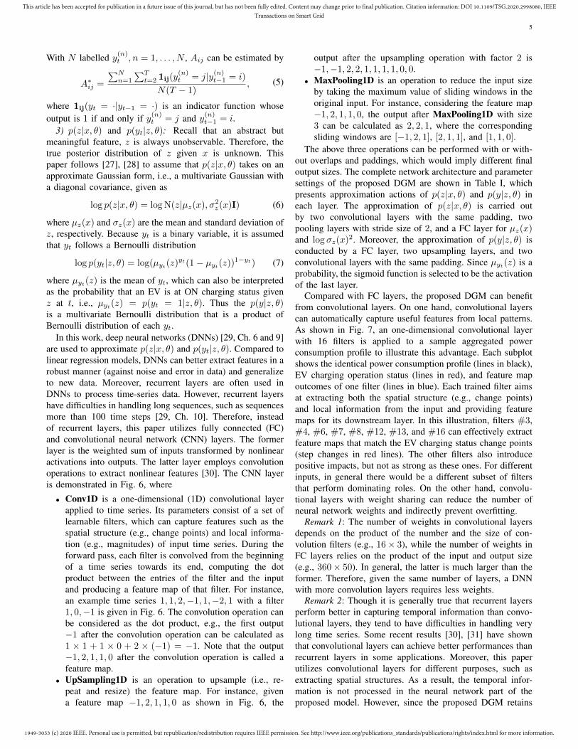
In this work, deep neural networks (DNNs) [29, Ch. 6 and 9]are used to approximate p(z|x, ✓) and p(yt|z, ✓). Compared tolinear regression models, DNNs can better extract features in arobust manner (against noise and error in data) and generalizeto new data. Moreover, recurrent layers are often used inDNNs to process time-series data. However, recurrent layershave difficulties in handling long sequences, such as sequencesmore than 100 time steps [29, Ch. 10]. Therefore, insteadof recurrent layers, this paper utilizes fully connected (FC)and convolutional neural network (CNN) layers. The formerlayer is the weighted sum of inputs transformed by nonlinearactivations into outputs. The latter layer employs convolutionoperations to extract nonlinear features [30]. The CNN layeris demonstrated in Fig. 6, where

• Conv1D is a one-dimensional (1D) convolutional layerapplied to time series. Its parameters consist of a set oflearnable filters, which can capture features such as thespatial structure (e.g., change points) and local informa-tion (e.g., magnitudes) of input time series. During theforward pass, each filter is convolved from the beginningof a time series towards its end, computing the dotproduct between the entries of the filter and the inputand producing a feature map of that filter. For instance,an example time series 1, 1, 2,�1, 1,�2, 1 with a filter1, 0,�1 is given in Fig. 6. The convolution operation canbe considered as the dot product, e.g., the first output�1 after the convolution operation can be calculated as1 ⇥ 1 + 1 ⇥ 0 + 2 ⇥ (�1) = �1. Note that the output�1, 2, 1, 1, 0 after the convolution operation is called afeature map.

• UpSampling1D is an operation to upsample (i.e., re-peat and resize) the feature map. For instance, givena feature map �1, 2, 1, 1, 0 as shown in Fig. 6, the

output after the upsampling operation with factor 2 is�1,�1, 2, 2, 1, 1, 1, 1, 0, 0.

• MaxPooling1D is an operation to reduce the input sizeby taking the maximum value of sliding windows in theoriginal input. For instance, considering the feature map�1, 2, 1, 1, 0, the output after MaxPooling1D with size3 can be calculated as 2, 2, 1, where the correspondingsliding windows are [�1, 2, 1], [2, 1, 1], and [1, 1, 0].

The above three operations can be performed with or with-out overlaps and paddings, which would imply different finaloutput sizes. The complete network architecture and parametersettings of the proposed DGM are shown in Table I, whichpresents approximation actions of p(z|x, ✓) and p(y|z, ✓) ineach layer. The approximation of p(z|x, ✓) is carried outby two convolutional layers with the same padding, twopooling layers with stride size of 2, and a FC layer for µz(x)and log �z(x)2. Moreover, the approximation of p(y|z, ✓) isconducted by a FC layer, two upsampling layers, and twoconvolutional layers with the same padding. Since µyt(z) is aprobability, the sigmoid function is selected to be the activationof the last layer.

Compared with FC layers, the proposed DGM can benefitfrom convolutional layers. On one hand, convolutional layerscan automatically capture useful features from local patterns.As shown in Fig. 7, an one-dimensional convolutional layerwith 16 filters is applied to a sample aggregated powerconsumption profile to illustrate this advantage. Each subplotshows the identical power consumption profile (lines in black),EV charging operation status (lines in red), and feature mapoutcomes of one filter (lines in blue). Each trained filter aimsat extracting both the spatial structure (e.g., change points)and local information from the input and providing featuremaps for its downstream layer. In this illustration, filters #3,#4, #6, #7, #8, #12, #13, and #16 can effectively extractfeature maps that match the EV charging status change points(step changes in red lines). The other filters also introducepositive impacts, but not as strong as these ones. For differentinputs, in general there would be a different subset of filtersthat perform dominating roles. On the other hand, convolu-tional layers with weight sharing can reduce the number ofneural network weights and indirectly prevent overfitting.

Remark 1: The number of weights in convolutional layersdepends on the product of the number and the size of con-volution filters (e.g., 16⇥ 3), while the number of weights inFC layers relies on the product of the input and output size(e.g., 360⇥ 50). In general, the latter is much larger than theformer. Therefore, given the same number of layers, a DNNwith more convolution layers requires less weights.

Remark 2: Though it is generally true that recurrent layersperform better in capturing temporal information than convo-lutional layers, they tend to have difficulties in handling verylong time series. Some recent results [30], [31] have shownthat convolutional layers can achieve better performances thanrecurrent layers in some applications. Moreover, this paperutilizes convolutional layers for different purposes, such asextracting spatial structures. As a result, the temporal infor-mation is not processed in the neural network part of theproposed model. However, since the proposed DGM retains

6

1 1 2 -1 1 -2 11 0 -1

-1 2 1 1 0

1×1 + 1×0 + 2×(−1)

Input Time Series

Filters (size=3)

Feature Map

Conv1D

-1 -1 2 2 1 1 1 1 0 0UpSampling1D (factor=2)

2 2 1

Copy (-1) twice

MaxPooling1D (size=3)

max(−1,2,1)

1 2

3

Fig. 6. Demonstration of a CNN layer, which consists of three sequential operations: Conv1D, UpSamping1D, and MaxPooling1D.

Filter #1

Filter #5

Filter #2 Filter #3 Filter #4

Filter #6 Filter #7 Filter #8

Filter #9 Filter #10 Filter #11 Filter #12

Filter #13 Filter #14 Filter #15 Filter #16

Aggregated powerconsumption profile

EV chargingstatus profile

Feature map ofconvolutional layer

Fig. 7. Visualization of feature maps extracted from convolutional layers with sixteen filters.

TABLE ITHE PROPOSED DGM ARCHITECTURE AND PARAMETER SETTINGS

Layer Name p(z|x, ✓) p(y|z, ✓)

Input 1440 50Layer1 Conv1D,16,3,ReLU FC,360,ReLULayer2 MaxPooling1D,2 UpSampling1D,2Layer3 Conv1D,1,3,ReLU Conv1D,16,3,ReLULayer4 MaxPooling1D,2 UpSampling1D,2Layer5 FC,50/50,- Conv1D,1,3,sigmoid

*Conv1D denotes 1D convolution layer followed by number and size offilters and an activation layer; MaxPooling1D denotes 1D max pooling layerfollowed by size of the max pooling windows; UpSampling1D denotes1D upsampling layer followed by upsampling factors; FC denotes a fullyconnected layer followed by number of neurons and an activation layer

the Markov property of HMMs, the corresponding temporalinformation is addressed by transition probabilities. In otherwords, convolutional layers with Markov property is proposedhere as an alternative of recurrent layers for time series.

C. Supervised Learning in DGM

With labelled dataset (X ,Y), ✓ in (6) and (7) can be deter-mined by maximum likelihood [26]. The marginal distributionof each (x, y) 2 (X ,Y) is obtained from the joint distribution(2) by marginalizing over the latent variable z

log p(x, y|✓) = log

Z

zp(x, y, z|✓)dz (8)

Maximizing (8) could lead to complicated expressions withno closed-form solutions since 1) the integral of the marginal

distribution is intractable when p(z|x, ✓) and p(y|z, ✓) areapproximated by DNNs with nonlinear hidden layers and2) batch optimization is costly for large amount of data.Following recent advances in variational inference [32], theproposed DGM can be trained by maximizing the evidencelower bound (ELBO) under data distribution. A lower boundL(✓|x, y) on the marginal distribution of (x, y) is given by

L(✓|x, y) = log p(x) + log p(y1) +TX

t=2

log p(yt|yt�1)

+TX

t=1

Ez⇠p(z|x,✓)⇥log p(yt|z, ✓)

⇤,

(9)

with proof given in the Appendix. Therefore, the ELBO underdata distribution x, y ⇠ pdata can be written as

L(✓|X ,Y) = Ex,y⇠pdata

⇥L(✓|x, y)

⇤. (10)

Then (6) and (7) can be trained by

✓⇤ = argmin

✓�L(✓|X ,Y) (11)

Since z is stochastic and thus gradients cannot be backpropa-gated, reparameterization is used to sample z, i.e., given x anda unit Gaussian noise ✏ ⇠ N(0, I), z = µz(x)+ ✏�z(x). Notethat the noises injected into the representation layer enablesthe proposed DGM to learn continuous feature representations.Note that such a sampling process of z is similar to thevariational autoencoder (VAE) [27]. Therefore, in this paperthe number of samples z is set to be 1 with a large minibatchsize Nb in accordance with the experimental setting in the



7

VAE. Based on (6), (7), and (11), it can be concluded that

✓⇤ = argmin

✓�

NbX

nb=1

TX

t=1

y(nb)t logµyt(z

(nb))

+ (1� y(nb)t ) log(1� µyt(z

(nb))) Loss

(12)

where z(nb) = µz(x(nb))+✏(nb)�z(x(nb)) and ✏

(nb) ⇠ N(0, I),x(nb) and y

(nb) are the nb-th instance from minibatch, z(nb)

is generated from x(nb), and y

(nb)t is the t-th element of

y(nb). From (12), it can be seen that the training objective is

to minimize the binary multi-label classification loss. In thispaper, p(z|x, ✓) and p(yt|z, ✓) are both differentiable functionscontaining different neural layers composed of multilayerperceptrons, convolution, max-pooling, upsampling, RectifiedLinear Units (ReLU), and sigmoid. Therefore, the gradient-descent based training methods Adam [33] is applied, whichis fairly insensitive to the choice of hyperparameters.

Furthermore, this paper utilizes the minibatch training, alsoknown as the minibatch gradient descent, which is a variationof the gradient descent algorithm that splits the trainingdataset into small batches. The implementation flowchart ofthe minibatch training in DGM is shown in Fig. 8. For eachbatch, the forward propagation first generates z and outputsµyt(z), and then the back propagation calculates model lossand update model weights.

V. THE PROPOSED DGM: EXACT INFERENCE

Once the proposed model is trained with �⇤, the next step is

to infer EV charging status y⇤ given aggregated consumption

profile x via maximizing a posteriori (MAP), i.e.,

y⇤ = argmax

yp(y|x,�⇤), (13)

which is approximated (with z sampled from p(z|x, ✓⇤)) by

y⇤ = argmax

ylog p(y1) +

TX

t=2

log p(yt|yt�1) +TX

t=1

log p(yt|z)

(14)Note that y⇤ in (14) can be further inferred via DP in two

stages. For forward induction, at each time step t, the first stepis to solve the following

Fc(t, yt) = minyt�1

{Fc(t� 1, yt�1)� log p(yt|z)

� log p(yt|yt�1)}(15)

where Fc(t, yt) is the optimal cost function over time steps t

and t� 1 given yt, and F (1, y1) = � log p(y1)� log p(y1|z).An example is shown in Fig. 9 to demonstrate the calculationof Fc(t, yt), where the values on the nodes are the cost(or values of the negative logarithm of posterior) and thevalues on the directed edges are the cost of transporting aunit from one node to the other (i.e., the negative logarithmof transition probability). Therefore, the overall process offorward induction is to find the minimum cost. Note that thecomplexity of this implementation is O(4T ).

For backward induction, the second step is solve the fol-lowing and find the minimum cost route,

y⇤t�1 = argmin

yt�1

{Fc(t� 1, yt�1)� log p(y⇤t |z)

� log p(y⇤t |yt�1)}(16)

where y⇤T = argminyT

F (T, yT ). The complexity of thisimplementation is O(2T ). Fig. 10 shows four typical inferenceresults corresponding to (a) once-charging , (b) twice-chargingin day and night, (c) twice-charging in two nights, and (d)multiple-charging, respectively. It can be observed that themeasured and inferred EV charging status are almost identical,which validates the effectiveness of the proposed framework.The incorporation of p(y1) and p(yt|yt�1) into the graphenables the model to consider the past events at the expenseof increased computational complexity of inference.

VI. NUMERIC RESULTS

In this section, the proposed algorithm is validated on thePecan Street dataset [34], which consists of measurementof circuit-level household electricity consumption data fromnearly 1,000 homes across the U.S. Each such home haveeight extra channels to record power consumption by majorappliances such as HVAC, refrigerators, and EVs.

A. Experiment Setup and Evaluation Metrics

The DGM in this paper is trained using Adam with an epochof 20, a mini-batch size of 100, and a learning rate of 0.001.All neuron weights are initialized using Glorot initialization[35]. After data pre-cleaning with removal of bad data points,the aggregated power consumption profiles and EV chargingprofiles are then standardized and binarized, respectively. Themain program is executed on an Intel i7-7820X 8-Core CPUwhile the training of the proposed DGM including the forwardand backward propagation is implemented on a TITAN XpGPU using TensorFlow as the computational framework. It isobserved that the loss of the model goes to convergence as theepoch increases, as shown in Fig. 11. To evaluate performanceof the proposed algorithm, the following classification metricsare employed,

Accuracy =TP + TN

TP + TN + FP + FN,

Recall =TP

TP + FN

Precision =TP

TP + FP,

F1 =2⇥ Precision⇥ Recall

Precision + Recallwhere

• TP is the true positive indicator, i.e., is the number ofcases where the DGM classifies the EV charging statusas ON and the actual status is indeed ON;

• TN is the true negative indicator, i.e., the number of caseswhere the DGM classifies the EV charging status as OFFand the actual status is indeed OFF;

• FP is the false positive indicator, i.e., the number of caseswhere the DGM classifies the EV charging status as ONbut the actual status is OFF; and

8

Start Set epochmax

epoch ≤ epochmaxEnd No

Shuffle historicaldata (#, %)

Yes

YesAll minibatches are traversed

Sample minibatch {(( )* , +()*))})*./0* from (#, %)

Output means {12(( )* )})*./0* and

standard deviations {32(( )* )})*./0* from 4(2|(, 6)

Sample noises {7 )* })*./0* from N(0, I)

Generate {2 )* })*./0* using reparameterization

Output {1+;(2 )* )})*./0* for ; = /: > from 4(+|2, 6)

6 can be updated for (14) using the Adam Algorithm

No

Fig. 8. Implementation flowchart of the minibatch training in DGM, including both forward and backward propagation.

!" = $

!" = %" = $ " = & " = ' " = (

)*(&, %)

)*(&, $)

− /012(!' = %|!& = $)

− /012(!' = %|!& = %)

)* ', % =min{)* &, % − /012 !' = % !& = % ,)* &, $ − /012 !' = % !& = $ }− /012(!' = %|4)

Fig. 9. Example demonstration of how to calculate Fc(t = 3, yt = 0) wherethe red sign highlights the possible minimum cost paths (the directed edges)from the last time step (t = 2) to the current time step (t = 3).

• FN is the false negative indicator, i.e., the number ofcases where the DGM classifies the EV charging statusas OFF but the actual status is ON.

B. EV Charging Status Classification

There are 93 houses with EV charging activities in the PecanStreet dataset, with one data point per minute per house. Witheach aggregated power consumption profile defined to be of 24hours, i.e., daily profiles. In this work, both transfer-learning-based and non-transfer-learning-based settings are utilized forthe purpose of comparison on performances. The differencebetween these two settings is that for non-transfer learning,the set of houses used in training is typically the same asthe set of houses used in testing. On the contrast, for transferlearning, the set of houses used in testing is typically differentfrom those used in training, which is a powerful method tocheck whether a certain model can “transfer” knowledge fromone dataset to another.

For the non-transfer learning setting, to reduce bias andvariance caused by the source data and better evaluate theeffectiveness of the proposed DGM, the five-fold cross-

validation (i.e., all available data is first shuffled and dividedinto five subsets, and each trial takes one subset for testingand the other four subsets for training) [26] is performed. Asshown in Fig. 12, the box plot and the green triangle are usedto visualize the variance and mean of evaluation results forthe following three scenarios, respectively.

• The first scenario is the proposed DGM without any noiseinjected into the test sets, denoted as “DGM w/o noise”;

• The second scenario is the proposed DGM with a Gaus-sian noise (zero mean and half standard deviation, i.e.,±0.5kW), denoted as “DGM w/ noise”;

• The third scenario is the HMM without any noise, de-noted as “HMM w/o noise”.

It can be observed that the variance of evaluation resultsis small for all five data partitions, and thus the proposedDGM is reasonably stable. On average, the proposed DGMincreases accuracy, precision, and F1 by 8.20%, 134.39%,56.43%, respectively, at the cost of reducing recall by 19.31%compared with the HMM on the five different data partitions.In terms of F1, the proposed DGM is better than the HMMwith better average performance of accuracy.

Furthermore, another comparative experiment is performedto demonstrate the robustness of the proposed DGM againstnoise in the data. From Fig. 12, the performance of theproposed DGM could be slightly affected by noise and error inthe data (the accuracy, precision, recall, and F1 drop by 0.82%,2.83%, 19.02%, and 13.61%). However, at a reasonable noiselevel, the proposed DGM still greatly outperforms HMM.Detailed evaluation results are provided in Table. II

For transfer learning setting, all data are split into thetraining dataset of 73 households and testing dataset shown inthe first column of Table III. For household with dataid 6871,it is an extreme case where there is no any EV charging events.From Table III, it is shown that the proposed DGM increases



9

Fig. 10. Selected typical examples of inference results including (a) once-charging, (b) twice-charging in day and night, (c) twice-charging in two nights,and (d) multiple-charging, respectively. Each row shows the aggregated power consumption profile, the probability of an EV at ON, the optimal cost overtime steps t and t� 1 given yt, the measured EV charging status profile, and the inferred EV charging status profile, respectively.

TABLE IIPERFORMANCE COMPARISON USING FIVE-FOLD CROSS-VALIDATION AND NON-TRANSFER LEARNING SETTING

Trial 1 Trial 2 Trial 3 Trial 4 Trial 5 Overall

Accuracy0.9794 /0.9692 /0.9055

0.9801 /0.9724 /0.9077

0.9802 /0.9763 /0.9084

0.9794 /0.9728 /0.9061

0.9809 /0.9692 /0.9058

0.9800±0.0006 /0.9720±0.0027 /0.9057±0.0011

Precision0.7683 /0.6348 /0.3409

0.8369 /0.8373 /0.3494

0.8306 /0.8275 /0.3527

0.7751 /0.7913 /0.3466

0.8169 /0.8233 /0.3417

0.8056±0.0285 /0.7828±0.0756 /0.3437±0.0045

Recall0.8318 /0.8818 /0.9822

0.7462 /0.5548 /0.9827

0.7613 /0.6700 /0.9820

0.8301 /0.6224 /0.9826

0.7894 /0.4765 /0.9819

0.7917±0.0035 /0.6411±0.1369 /0.9812±0.0004

F1 Score0.7978 /0.7370 /0.5061

0.7879 /0.6661 /0.5155

0.7935 /0.7394 /0.5190

0.8006 /0.6953 /0.5124

0.8021 /0.6021 /0.5070

0.7964±0.0052 /0.6880±0.0509 /0.5091±0.0049

Note that top/middle/bottom numbers in each cell represent metrics of DGM w/o noise, DGM w/ noise, and HMM w/o noise, repsectively.

Fig. 11. Illustration of convergence of the training (black line) and validation(blue line) losses as the epochs increase during training.

accuracy, precision, and F1 by 10.8%, 89% and 42.8% at thecost of reducing recall by 17.2% compared with the HMM.In terms of F1, DGM is better than HMM with high averageperformance of accuracy.

Compared to HMMs, it can be observed that the proposedDGM achieved better performance in accuracy, precision,and F1 but only received a lower score in recall under bothsettings. That is because that HMMs cannot accurately classifythe EV charging status as “OFF”, i.e., HMMs classifies most“OFF” statuses as “ON” wrongly while the proposed DGMmethod can mitigate this issue of the HMM method at the cost

of classifying a small number of “ON” statuses as “OFF”.

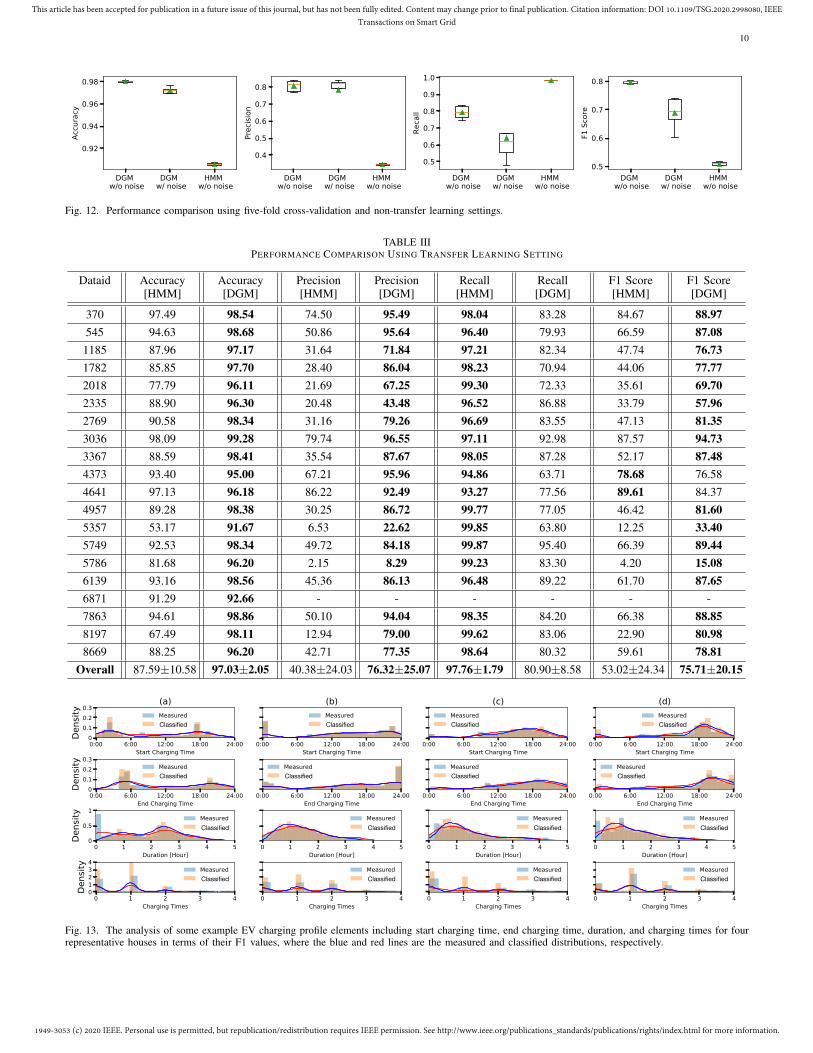
C. EV Charging Profile Elements Analyses

Four houses (dataid 3036 (a), 370 (b), 1782 (c), and2018 (d)) are selected according to their different F1 valuesfrom high to low. Four elements of EV charging profilesare extracted from measured and corresponding classified EVcharging status. Once the extracted results are collected, thedistribution of EV charging profile elements can be visualizedby Gaussian mixture. As shown in Fig.13, the distribution ofEV charging profile elements from measured and classifiedresults are represented by the blue and red lines respectively.For each household, it can be seen that the red line isalmost identical to the blue line. That is, the distributionof the measured elements can be well approximated by theclassified elements. Therefore, the proposed framework isaccurate and effective. According to the distribution of theclassified elements, it can be summarized that most householdscharge their EVs after work around 6 p.m and also tend tocharge their EVs for one hour and once per day. So theseinformation can be further analyzed to achieve more accurateEV charging profiles.



10

Fig. 12. Performance comparison using five-fold cross-validation and non-transfer learning settings.

TABLE IIIPERFORMANCE COMPARISON USING TRANSFER LEARNING SETTING

Dataid Accuracy[HMM]

Accuracy[DGM]

Precision[HMM]

Precision[DGM]

Recall[HMM]

Recall[DGM]

F1 Score[HMM]

F1 Score[DGM]

370 97.49 98.54 74.50 95.49 98.04 83.28 84.67 88.97545 94.63 98.68 50.86 95.64 96.40 79.93 66.59 87.08

1185 87.96 97.17 31.64 71.84 97.21 82.34 47.74 76.731782 85.85 97.70 28.40 86.04 98.23 70.94 44.06 77.772018 77.79 96.11 21.69 67.25 99.30 72.33 35.61 69.702335 88.90 96.30 20.48 43.48 96.52 86.88 33.79 57.962769 90.58 98.34 31.16 79.26 96.69 83.55 47.13 81.353036 98.09 99.28 79.74 96.55 97.11 92.98 87.57 94.733367 88.59 98.41 35.54 87.67 98.05 87.28 52.17 87.484373 93.40 95.00 67.21 95.96 94.86 63.71 78.68 76.584641 97.13 96.18 86.22 92.49 93.27 77.56 89.61 84.374957 89.28 98.38 30.25 86.72 99.77 77.05 46.42 81.605357 53.17 91.67 6.53 22.62 99.85 63.80 12.25 33.405749 92.53 98.34 49.72 84.18 99.87 95.40 66.39 89.445786 81.68 96.20 2.15 8.29 99.23 83.30 4.20 15.086139 93.16 98.56 45.36 86.13 96.48 89.22 61.70 87.656871 91.29 92.66 - - - - - -7863 94.61 98.86 50.10 94.04 98.35 84.20 66.38 88.858197 67.49 98.11 12.94 79.00 99.62 83.06 22.90 80.988669 88.25 96.20 42.71 77.35 98.64 80.32 59.61 78.81

Overall 87.59±10.58 97.03±2.05 40.38±24.03 76.32±25.07 97.76±1.79 80.90±8.58 53.02±24.34 75.71±20.15

Classified

Classified

Classified

Classified

Classified

Classified

Classified

Classified

Classified

Classified

Classified

Classified

Classified

Classified

Classified

Classified

Fig. 13. The analysis of some example EV charging profile elements including start charging time, end charging time, duration, and charging times for fourrepresentative houses in terms of their F1 values, where the blue and red lines are the measured and classified distributions, respectively.



11

VII. CONCLUSION

This paper proposed a DGM driven non-intrusive identifi-cation framework for EV charging profile. With the capabilityof complex density estimation by DGMs, the EV chargingstatus can be modeled and inferred from DGMs via DP. ThenEV charging profiles can be reconstructed according to therated power of EV models and inferred status. Experiments onPecan Street datasets were conducted to validate the feasibilityand effectiveness of the proposed framework. The numericalresults show that the proposed method can improve the overallperformance compared with the state-of-art HMMs, though adecrease in the recall was observed. In addition, the proposedframework can well handle noisy and unseen data and thuspossesses improved robustness and generalization capabilities.For future research, the proposed framework can be extendedto more general multi-class multi-label classification tasks.

APPENDIX APROOF OF ELBO (9)

Proof: Inserting (2) into (8) implies

log p(x, y|✓) = log

Z

zp(x)p(y1)

TY

t=2

p(yt|yt�1)

p(z|x, ✓)TY

t=1

p(yt|z, ✓)dz

= log p(x) + log p(y1) +TX

t=2

log p(yt|yt�1)

+TX

t=1

log(Ez⇠p(z|x,✓)[p(yt|z, ✓)])

(17)According to Jensen’s Inequality, (17) implies

log p(x, y|✓) � log p(x) + log p(y1) +TX

t=2

log p(yt|yt�1)

+TX

t=1

Ez⇠p(z|x,✓)[log p(yt|z, ✓)].

(18)

REFERENCES

[1] U.S. Energy Information Admin., “Annual Energy Outlook,” 2019.[2] D. Gohlke and Y. Zhou, “Impacts of electrification of light-duty vehicles

in the U.S., 2010-2017,” Argonne National Lab, Tech. Rep., 2018.[3] P. G. Pereirinha, M. Gonzalez, I. Carrilero, D. Ansean, J. Alonso,

and J. C. Viera, “Main trends and challenges in road transportationelectrification,” Transport. Res. Procedia, vol. 33, pp. 235–242, 2018.

[4] A. Dubey and S. Santoso, “Electric vehicle charging on residentialdistribution systems: Impacts and mitigations,” IEEE Access, vol. 3, pp.1871–1893, 2015.

[5] S. Huang and Q. Wu, “Dynamic tariff-subsidy method for pv and v2gcongestion management in distribution networks,” IEEE Trans. Smart

Grid, vol. 10, no. 5, pp. 5851–5860, Sep. 2019.[6] B. Zhang and M. Kezunovic, “Impact on power system flexibility by

electric vehicle participation in ramp market,” IEEE Trans. Smart Grid,vol. 7, no. 3, pp. 1285–1294, May 2016.

[7] Z. Liu, Q. Wu, K. Ma, M. Shahidehpour, Y. Xue, and S. Huang,“Two-stage optimal scheduling of electric vehicle charging based ontransactive control,” IEEE Trans. Smart Grid, vol. 10, no. 3, pp. 2948–2958, 2019.

[8] K. Qian, C. Zhou, M. Allan, and Y. Yuan, “Modeling of load demanddue to ev battery charging in distribution systems,” IEEE Trans. Power

Syst., vol. 26, no. 2, pp. 802–810, May 2011.[9] D. Tang and P. Wang, “Nodal impact assessment and alleviation of

moving electric vehicle loads: From traffic flow to power flow,” IEEE

Trans. Power Sys., vol. 31, no. 6, pp. 4231–4242, 2016.[10] Y. Cao, S. Tang, C. Li, P. Zhang, Y. Tan, Z. Zhang, and J. Li, “An

optimized ev charging model considering tou price and soc curve,” IEEE

Trans. Smart Grid, vol. 3, no. 1, pp. 388–393, 2011.[11] S. Shao, M. Pipattanasomporn, and S. Rahman, “Grid integration of

electric vehicles and demand response with customer choice,” IEEE

Trans. Smart Grid, vol. 3, no. 1, pp. 543–550, 2012.[12] J. Zheng, X. Wang, K. Men, C. Zhu, and S. Zhu, “Aggregation model-

based optimization for electric vehicle charging strategy,” IEEE Trans.

Smart Grid, vol. 4, no. 2, pp. 1058–1066, June 2013.[13] A. Y. Lam, K.-C. Leung, and V. O. Li, “Capacity estimation for vehicle-

to-grid frequency regulation services with smart charging mechanism,”IEEE Trans. Smart Grid, vol. 7, no. 1, pp. 156–166, 2015.

[14] M. G. Flammini, G. Prettico, A. Julea, G. Fulli, A. Mazza, andG. Chicco, “Statistical characterisation of the real transaction datagathered from electric vehicle charging stations,” Electric Power Systems

Research, vol. 166, pp. 136–150, 2019.[15] E. Xydas, C. Marmaras, L. M. Cipcigan, N. Jenkins, S. Carroll, and

M. Barker, “A data-driven approach for characterising the chargingdemand of electric vehicles: A UK case study,” Applied energy, vol.162, pp. 763–771, 2016.

[16] Y. B. Khoo, C.-H. Wang, P. Paevere, and A. Higgins, “Statisticalmodeling of electric vehicle electricity consumption in the Victorian EVtrial, Australia,” Transport. Res. Part D, vol. 32, pp. 263–277, 2014.

[17] E. C. Kara, J. S. Macdonald, D. Black, M. Berges, G. Hug, andS. Kiliccote, “Estimating the benefits of electric vehicle smart chargingat non-residential locations: A data-driven approach,” Applied Energy,vol. 155, pp. 515–525, 2015.

[18] S. Wang, L. Du, J. Ye, and D. Zhao, “Robust identification of EVcharging profiles,” in 2018 IEEE Transportation Electrification Conf.

Expo. (ITEC). IEEE, 2018.[19] Z. Zhang, J. H. Son, Y. Li, M. Trayer, Z. Pi, D. Y. Hwang, and J. K.

Moon, “Training-free non-intrusive load monitoring of electric vehiclecharging with low sampling rate,” in 40th Annual Conference of the

IEEE Industrial Electronics Society, Oct 2014, pp. 5419–5425.[20] A. A. Munshi and Y. A.-R. I. Mohamed, “Unsupervised nonintrusive

extraction of electrical vehicle charging load patterns,” IEEE Trans Ind.

Informat., vol. 15, no. 1, pp. 266–279, 2019.[21] Q. Dang, Y. Huo, and C. Sun, “Privacy preservation needed for smart

meter system: A methodology to recognize electric vehicle (EV) mod-els,” in 2018 IEEE ISGT-ASIA. IEEE, 2018, pp. 1016–1020.

[22] H. Zhao, X. Yan, and L. Ma, “Training-free non-intrusive load extractingof residential electric vehicle charging loads,” IEEE Access, vol. 7, pp.117 044–117 053, 2019.

[23] O. Parson, S. Ghosh, M. Weal, and A. Rogers, “Non-intrusive loadmonitoring using prior models of general appliance types,” in Twenty-

Sixth AAAI Conference on Artificial Intelligence, 2012.[24] V. Hoffmann, B. I. Fesche, K. Ingebrigtsen, I. N. Christie, and M. Pun-

nerud Engelstad, “Automated detection of electric vehicles in hourlysmart meter data,” IEEE Access, 2019.

[25] Z. Ghahramani, “An introduction to hidden markov models and bayesiannetworks,” in Hidden Markov models: applications in computer vision.World Scientific, 2001, pp. 9–41.

[26] C. M. Bishop, Pattern recognition & machine learning. Springer, 2006.[27] D. P. Kingma and M. Welling, “Stochastic gradient vb and the varia-

tional auto-encoder,” in Second International Conference on Learning

Representations, ICLR, vol. 19, 2014.[28] D. I. J. Im, S. Ahn, R. Memisevic, and Y. Bengio, “Denoising criterion

for variational auto-encoding framework,” in Thirty-First AAAI Confer-

ence on Artificial Intelligence, 2017.[29] I. Goodfellow, Y. Bengio, and A. Courville, Deep learning. MIT press,

2016.[30] H. I. Fawaz, G. Forestier, J. Weber, L. Idoumghar, and P.-A. Muller,

“Deep learning for time series classification: a review,” Data Mining

and Knowledge Discovery, vol. 33, no. 4, pp. 917–963, 2019.[31] J. Kelly and W. Knottenbelt, “Neural nilm: Deep neural networks

applied to energy disaggregation,” in Proceedings of the 2nd ACM

International Conference on Embedded Systems for Energy-Efficient

Built Environments. ACM, 2015, pp. 55–64.[32] C. Zhang, J. Butepage, H. Kjellstrom, and S. Mandt, “Advances in

variational inference,” IEEE Trans. Pattern Anal. Mach. Intell., 2019.



12

[33] D. P. Kingma and J. Ba, “Adam: A method for stochastic optimization,”arXiv preprint arXiv:1412.6980, 2014.

[34] “Pecan street database,” http://www.pecanstreet.org. [Online]. Available:http://www.pecanstreet.org/

[35] X. Glorot and Y. Bengio, “Understanding the difficulty of training deepfeedforward neural networks,” in Proceedings of the 13th international

conf. artificial intelligence and statistics, 2010, pp. 249–256.

Shengyi Wang (S’17) received the B.S. and M.S.degrees in electrical engineering from ShanghaiUniversity of Electric Power, China, and ClarksonUniversity, Potsdam, NY, in 2016 and 2017, respec-tively. He is currently pursuing his Ph.D. degree atTemple University, Philadelphia. He received Out-standing Undergraduate Thesis Award in 2016. Hewas a summer Research Intern at Global Energy In-terconnection Research Institute North America (SanJose, CA) and at Mitsubishi Electric Research Labs(Cambridge, MA), in 2019 and 2020, respectively.

His research interests include game-theoretic control for multi-agent sys-tems, data-driven optimization for power systems, and non-intrusive loadmonitoring.

Liang Du (S’09–M’13–SM’18) received the Ph.D.degree in electrical engineering from Georgia Insti-tute of Technology, Atlanta, GA in 2013. He wasa Research Intern at Eaton Corp. Innovation Cen-ter (Milwaukee, WI), Mitsubishi Electric ResearchLabs (Cambridge, MA), and Philips Research N.A.(Briarcliff Manor, NY) in 2011, 2012, and 2013,respectively. He was also an Electrical Engineerwith Schlumberger, Sugar Land, TX, from 2013 to2017. He is currently an Assistant Professor withTemple University, Philadelphia. Dr. Du received the

Ralph E. Powe Junior Faculty Enhancement Award from ORAU in 2018and currently serve as an associate editor for IEEE TRANSACTIONS ON IN-DUSTRY APPLICATIONS and IEEE TRANSACTIONS ON TRANSPORTATIONELECTRIFICATION.

Jin Ye (S’13-M’14-SM’16) received the B.S. andM.S. degrees in electrical engineering from Xi’anJiaotong University, China, in 2008 and 2011, re-spectively. She received her Ph.D. degree in electri-cal engineering from McMaster University, Canadain 2014. She is currently an assistant professor ofelectrical engineering and the director of intelligentpower electronics and electric machines (IPEM)laboratory at the University of Georgia. Her mainresearch areas include power electronics, electricmachines, energy management systems, and cyber-

physical security and resilience with applications to smart grids and electrifiedtransportation.

Dr. Ye was the general chair of 2019 IEEE Transportation Electrifica-tion Conference and Expo (ITEC) and a publication chair and women inengineering chair of 2019 IEEE Energy Conversion Congress and Expo(ECCE). She serves as a steering committee member for the cyber-physicalsecurity initiative for the IEEE Power Electronics Society (PELS), a PELSrepresentative for the Transportation Electrification Community (TEC), andTEC representative for PELS Technical Committee on Transportation andVehicle Systems. She is an associate editor for IEEE TRANSACTIONS ONPOWER ELECTRONICS, IEEE OPEN JOURNAL OF POWER ELECTRONICS,IEEE TRANSACTIONS ON TRANSPORTATION ELECTRIFICATION, and IEEETRANSACTIONS ON VEHICULAR TECHNOLOGY.

Dongbo Zhao (SM’16) received his B.S. degreesfrom Tsinghua University, Beijing, China, the M.S.degree from Texas A&M University, College Sta-tion, Texas, and the Ph.D. degree from Georgia Insti-tute of Technology, Atlanta, Georgia, all in electricalengineering. He has worked with Eaton Corpora-tion from 2014 to 2016 as a Lead Engineer in itsCorporate Research and Technology Division, andwith ABB in its US Corporate Research Center from2010 to 2011. Currently he is a Principal EnergySystem Scientist with Argonne National Laboratory,

Lemont, IL. He is also an Institute Fellow of Northwestern Argonne Instituteof Science and Engineering of Northwestern University. His research interestsinclude power system control, protection, reliability analysis, transmission anddistribution automation, and electric market optimization.

Dr. Zhao is the editor of IEEE TRANSACTIONS ON POWER DELIVERY,IEEE TRANSACTIONS ON SUSTAINABLE ENERGY, and IEEE POWER EN-GINEERING LETTERS. He is the subject editor of subject “Power systemoperation and planning with renewable power generation” of IET RenewablePower Generation and the Associate Editor of IEEE ACCESS.

Documents

A Deep Generative Model for Non-intrusive Identification