A. DDPM TRAINING AND SAMPLING

To train and sample from our diffusion model, we use thealgorithms as described in [8].

Algorithm 2 TrainingInput: q(x0), N steps, noise schedule β1, ..., βNrepeatx0 ∼ q(x0)t ∼ U({1, ..., N})√α ∼ U(

√αt−1,

√αt)

ε ∼ N (0, I)Take gradient descent step on∇θ

∥∥ε− εθ(√αtx0 +√

1− αtε,√α)

∥∥2

until converged

Algorithm 3 SamplingInput: N steps, noise schedule β1, ..., βNxN ∼ N (0, I)for t = N, ..., 1 doε ∼ N (0, I) if t > 1, else ε = 0

xt−1 = 1√αt

(xt − 1−αt√

1−αtεθ(xt,

√αt)

)+ σtε

end forreturn x0

B. MUSICVAE ARCHITECTURE

Z

♪ ♪ ♪

Encoder

Latent Code

Input

Output

♪

Decoder

Figure 4. 2-bar melody MusicVAE architecture. The en-coder is a bi-direction LSTM and the decoder is an autore-gressive LSTM.

C. TRIMMING LATENTS

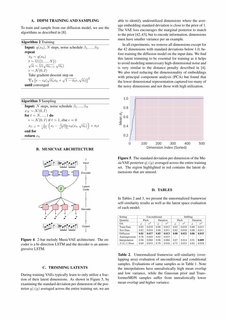
During training VAEs typically learn to only utilize a frac-tion of their latent dimensions. As shown in Figure 5, byexamining the standard deviation per dimension of the pos-terior q(z|y) averaged across the entire training set, we are

able to identify underutilized dimensions where the aver-age embedding standard deviation is close to the prior of 1.The VAE loss encourages the marginal posterior to matchto the prior [42,43], but to encode information, dimensionsmust have smaller variance per an example.

In all experiments, we remove all dimensions except forthe 42 dimensions with standard deviations below 1.0, be-fore training the diffusion model on the input data. We findthis latent trimming to be essential for training as it helpsto avoid modeling unnecessary high-dimensional noise andis very similar to the distance penalty described in [4].We also tried reducing the dimensionality of embeddingswith principal component analysis (PCA) but found thatthe lower dimensional representation captured too many ofthe noisy dimensions and not those with high utilization.

0 100 200 300 400 500Dimension Index (Sorted)

0.2

0.4

0.6

0.8

1.0

Mea

n z

Figure 5. The standard deviation per dimension of the Mu-sicVAE posterior q(z|y) averaged across the entire trainingset. The region highlighted in red contains the latent di-mensions that are unused.

D. TABLES

In Tables 2 and 3, we present the unnormalized framewiseself-similarity results as well as the latent space evaluationof each model.

Setting Unconditional InfillingQuantity Pitch Duration Pitch DurationOA µ σ2 µ σ2 µ σ2 µ σ2

Train Data 0.82 0.018 0.88 0.012 0.82 0.018 0.88 0.012Test Data 0.82 0.018 0.88 0.011 0.82 0.018 0.88 0.011Diffusion 0.81 0.017 0.85 0.013 0.80 0.021 0.86 0.015Autoregression 0.76 0.024 0.82 0.015 - - - -Interpolation 0.94 0.004 0.96 0.004 0.87 0.014 0.91 0.009N (0, I) Prior 0.69 0.033 0.79 0.016 0.73 0.033 0.82 0.018

Table 2. Unnormalized framewise self-similarity (over-lapping area) evaluation of unconditional and conditionalsamples. Evaluations of same samples as in Table 1. Notethe interpolations have unrealistically high mean overlapand low variance, while the Gaussian prior and Trans-formerMDN samples suffer from unrealistically lowermean overlap and higher variance.

Setting Unconditional InfillingMetric FD×10−2 MMD×10−2 FD×10−2 MMD×10−2

Train Data 0.00 0.00 0.00 0.00Test Data 1.24 0.12 1.24 0.12Diffusion 1.66 0.18 1.53 0.16Autoregression 1.26 0.12 - -Interpolation 3.22 0.43 1.97 0.23N (0, I) Prior 2.44 0.29 1.17 0.12

Table 3. Latent space evaluation of infilling and uncon-ditional and conditional samples. As described in Sec-tion 4.5, the TransformerMDN performs better in latentspace similarity, even while producing less realistic sam-ples (as seen in Tables 1 and 2).

E. ADDITIONAL SAMPLES

In Figure 6 we provide piano rolls of sequences drawnfrom the test set and in Figures 7, 8, 9, and 10 we presentadditional samples unconditionally generated by our dif-fusion model, TransformerMDN, spherical interpolation,and through independent sampling from the MusicVAEprior, respectively. Additional piano roll visualizationsfrom infilling experiments are provided in Figure 11.

For extended visual and audio samples of thegenerated sequences from each model, we referthe reader to the online supplement available athttps://goo.gl/magenta/symbolic-music-diffusion-examples.

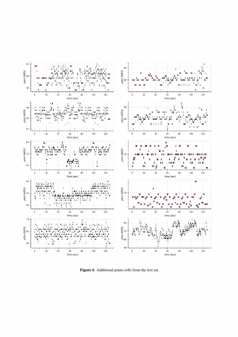
Figure 6. Additional piano rolls from the test set.

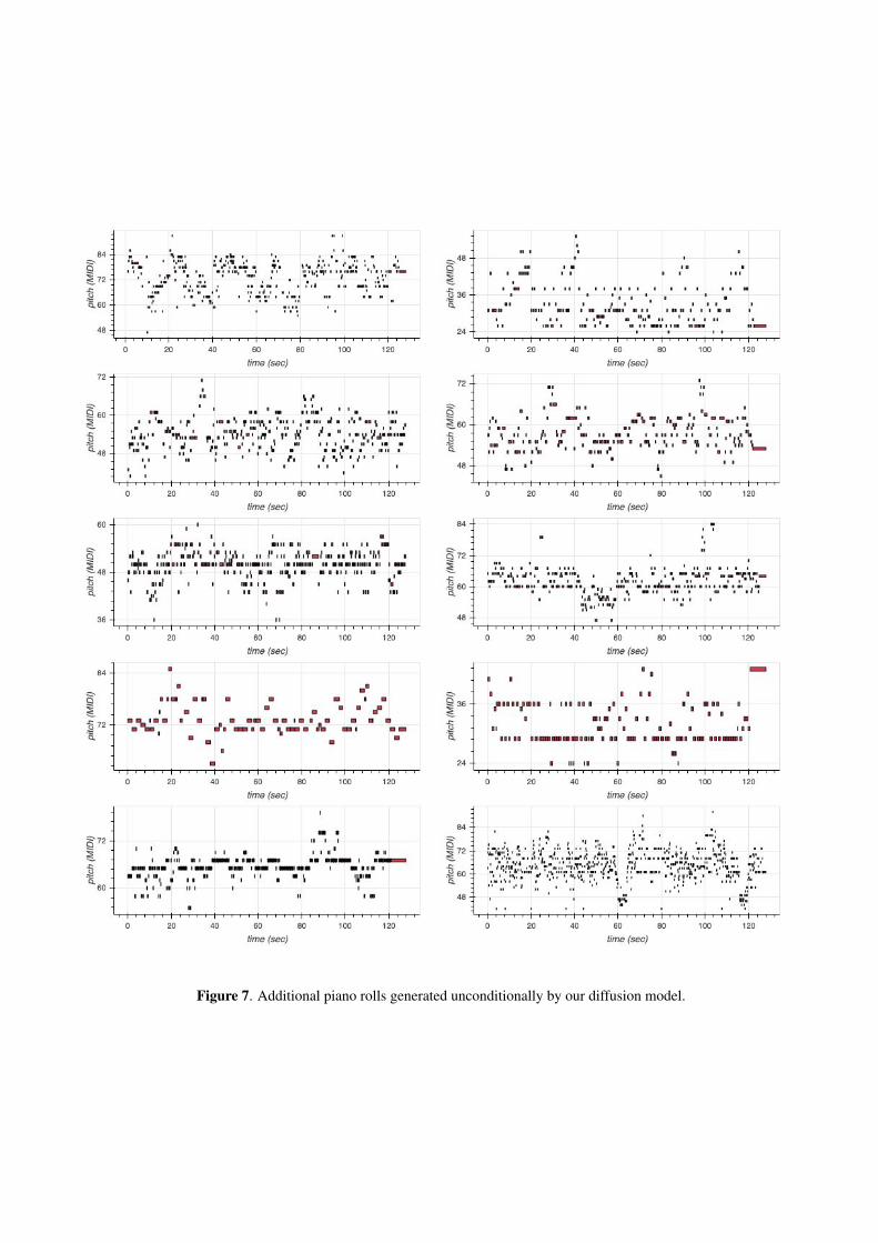
Figure 7. Additional piano rolls generated unconditionally by our diffusion model.

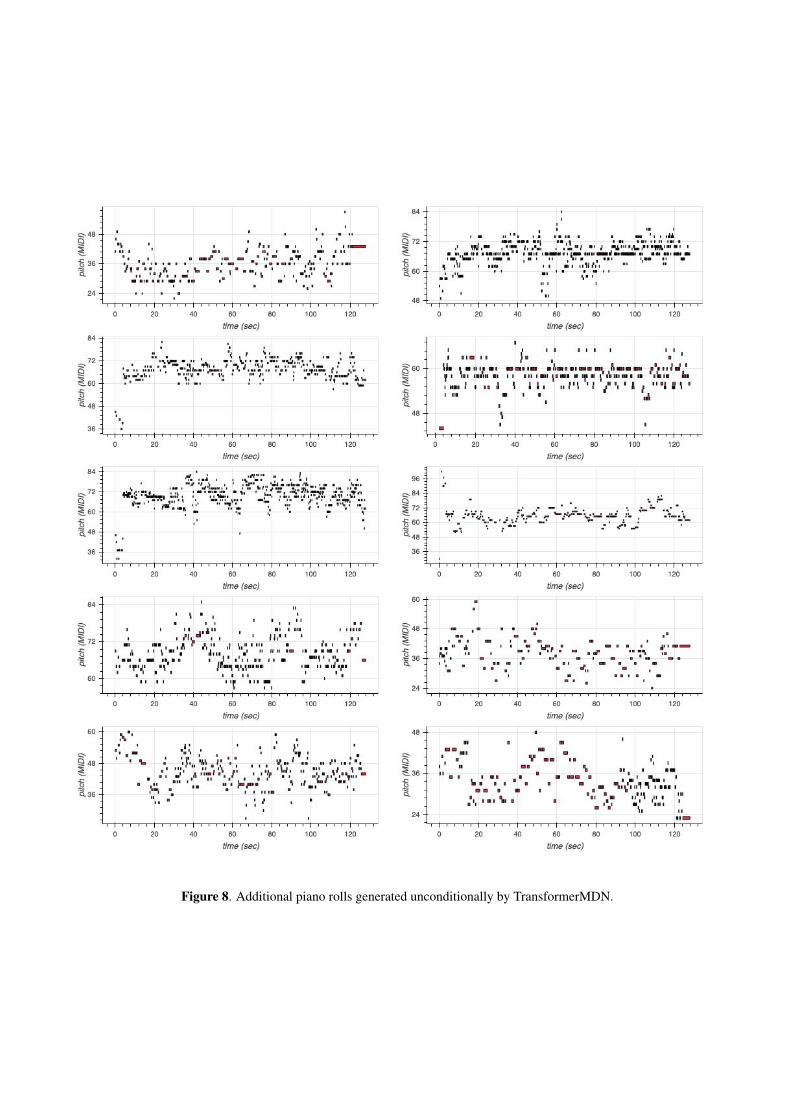
Figure 8. Additional piano rolls generated unconditionally by TransformerMDN.

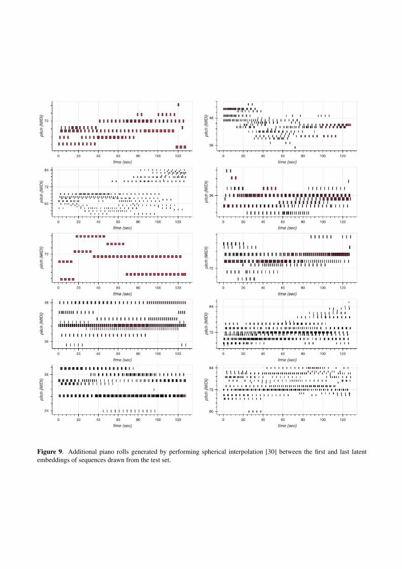
Figure 9. Additional piano rolls generated by performing spherical interpolation [30] between the first and last latentembeddings of sequences drawn from the test set.

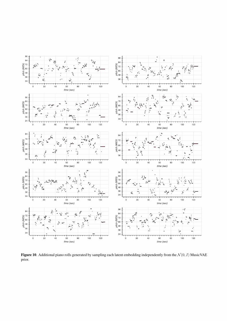
Figure 10. Additional piano rolls generated by sampling each latent embedding independently from theN (0, I) MusicVAEprior.

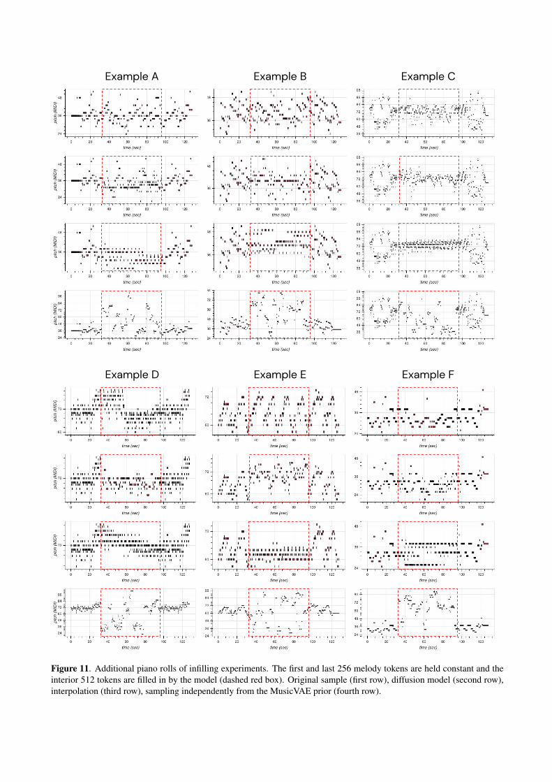
Example A Example B Example C

Example D Example E Example F

Figure 11. Additional piano rolls of infilling experiments. The first and last 256 melody tokens are held constant and theinterior 512 tokens are filled in by the model (dashed red box). Original sample (first row), diffusion model (second row),interpolation (third row), sampling independently from the MusicVAE prior (fourth row).