A critical overview of machining simulations in ABAQUS866670/FULLTEXT01.pdf · DEGREE PROJECT, IN SOLID MECHANICS , SECOND LEVEL STOCKHOLM, SWEDEN 2014 A critical overview of machining

DEGREE PROJECT, IN , SECOND LEVELSOLID MECHANICS

STOCKHOLM, SWEDEN 2014

A critical overview of machiningsimulations in ABAQUS

MIKAELA ZETTERBERG

KTH ROYAL INSTITUTE OF TECHNOLOGY

ENGINEERING SCIENCES

A critical overview of machining simulations in ABAQUSAuthor: M. Zetterberg

Report No: KIMAB-2014-127 Swerea KIMAB Project No: 11187

Status: Open Date: 2014-11-20

Abstract

Metal cutting is one of the mostcommonly occurring manufacturingprocesses in the industry and ma-jor effort is made to improve its pro-cesses. Cutting tools are expensiveand have a life length measured inminutes, why predictions of tool wearare of great interest. Finite Ele-ment (FE) simulations have a cen-tral role in the development of toolsand cutting processes, but perform-ing simulations of metal cutting isnot easy. The method chosen forthe chip formation has a large im-pact on the result of the simulations.The scope of this work includes asurvey on important parameters anddifferent possibilities to form a chipin simulations of metal cutting inABAQUS/Explicit. Particular em-phases are placed the on predictionof flank wear and how the hard-ening implemented in the materialmodel effects this. The approach hasbeen to start with a literature studyand thereafter make simulations inABAQUS/Explicit. FE simulations,of cutting, with different damagecriteria and simulations with SPH(Smooth Particle Hydrodynamics)-method are presented. None ofthe possibilities to form a chip inABAQUS/Explicit, as implementedtoday, seems to be sufficient for sim-

ulations of cutting to predict flankwear. The SPH-method will be agood alternative for simulations ofmetal cutting in ABAQUS/Explicitif temperature dependency is imple-mented. The material model in gen-eral, the type of hardening in specific,has an impact on the chip-form andthe stress state in the chip and work-piece. And thereby effects the flankwear.

c© Swerea KIMAB AB • KIMAB-2014-127

Abstract in Swedish

Skärande bearbetning är en av devanligast förekommande tillverkn-ingsprocesserna i industrin idag ochmycket möda läggs ned för att för-bättra dess processer. Skären ärdyra och har en livslängd som kanmätas i minuter, vilket gör att möj-ligheten att förstå och förutsäga nöt-ningen av skäret är av stort intresse.Finita element (FE) simuleringarhar en central roll i utvecklingenav skärverktyg och skär processer,men att genomföra simuleringar avdetta är långt ifrån enkelt. Meto-den som väljs, för att forma enspåna har stor påverkan på resul-tatet av simuleringarna. Detta ar-bete innefattar en utredning kringviktiga parametrar och olika möj-ligheter att åstadkomma spånformn-ing vid simuleringar av skärandebearbetning i ABAQUS/Explicit.Särskiljt har fokus legat på att kunnaförutsäga nötning på skärets släpp-

sida och hur hårdnandet, som finnsimplementerat i materialmodellen,påverkar denna. Angreppssättethar varit att starta med en litter-aturstudie och därefter göra simu-lationer i ABAQUS/Explicit. Re-sultat från FE simuleringar, avskärande bearbetning, med olikabrottvillkor och simuleringar medSmooth Particle Hydrodynamics(SPH)- metoden finns presenterade.Ingen av möjligheterna för spån-formning som finns implementeradei ABAQUS/Explicit idag är tillräck-ligt bra för att simulera nötning avskärets släppsida. SPH-metodenkan komma att bli ett bra alter-nativ för simuleringar av skärandebearbetning i ABAQUS/Explicitom temperaturberoendet blir im-plementerat. Materialmodellen,och mer specifikt typen av hård-nande, påverkar spånformen ochspänningstillståndet i spånan och ar-betsstycket. Därmed påverkas ocksånötningen av skäret.

Swerea KIMAB AB, Box 55970, SE-102 16 Stockholm, SwedenTel. +46 (0)8-440 48 00 • Fax +46 (0)8-440 45 35 • E-mail [email protected] • www.swerea.se


Contents

1 Introduction 11.1 Aim . . . . . . . . . . . . . . . . . . . . . . . . . . . . . . . . 11.2 Methodology . . . . . . . . . . . . . . . . . . . . . . . . . . . 1

2 Basic concepts of machining processes 22.1 Geometric description of orthogonal machine cutting . . . . . 22.2 Deformation zones . . . . . . . . . . . . . . . . . . . . . . . . 22.3 Friction . . . . . . . . . . . . . . . . . . . . . . . . . . . . . . 42.4 Chip formation process . . . . . . . . . . . . . . . . . . . . . . 42.5 Thermal processes . . . . . . . . . . . . . . . . . . . . . . . . 4

2.5.1 Heat production . . . . . . . . . . . . . . . . . . . . . 52.5.2 Thermal effects in the workpiece and tool material . . 5

2.6 Tool wear . . . . . . . . . . . . . . . . . . . . . . . . . . . . . 62.6.1 Tool wear mechanisms . . . . . . . . . . . . . . . . . . 62.6.2 Types of tool wear . . . . . . . . . . . . . . . . . . . . 6

3 Finite Element Simulation of metal cutting 73.1 Arbitrary Lagrangian-Eulerian adaptive meshing . . . . . . . 7

3.1.1 Boundaries in ALE methods . . . . . . . . . . . . . . 93.1.2 Mesh-update procedures . . . . . . . . . . . . . . . . . 93.1.3 Motion in ALE . . . . . . . . . . . . . . . . . . . . . . 103.1.4 Stress-update procedures . . . . . . . . . . . . . . . . 10

3.2 Chip - workpiece separation in an FE environment . . . . . . 103.2.1 Adaptive Meshing . . . . . . . . . . . . . . . . . . . . 113.2.2 Element failure models . . . . . . . . . . . . . . . . . . 133.2.3 SPH simulation of metal cutting . . . . . . . . . . . . 133.2.4 Eulerian models . . . . . . . . . . . . . . . . . . . . . 143.2.5 Path dependent parting . . . . . . . . . . . . . . . . . 14

3.3 Friction models . . . . . . . . . . . . . . . . . . . . . . . . . . 153.3.1 Coulomb friction model . . . . . . . . . . . . . . . . . 153.3.2 Constant shear model . . . . . . . . . . . . . . . . . . 153.3.3 Sticking zone and sliding zone model . . . . . . . . . . 163.3.4 Friction in smooth particle hydrodynamic simulations 16

3.4 Heat transfer models . . . . . . . . . . . . . . . . . . . . . . . 163.4.1 Adiabatic assumption . . . . . . . . . . . . . . . . . . 163.4.2 Coupled Thermal-Stress analysis . . . . . . . . . . . . 17


3.5 FE models of tool wear . . . . . . . . . . . . . . . . . . . . . 17

3.5.1 Tool wear rate models . . . . . . . . . . . . . . . . . . 17

3.5.2 Cyclic implementation . . . . . . . . . . . . . . . . . . 18

4 Material models 18

4.1 Hardening . . . . . . . . . . . . . . . . . . . . . . . . . . . . . 18

4.1.1 Yield criterion . . . . . . . . . . . . . . . . . . . . . . 18

4.1.2 Flow rule . . . . . . . . . . . . . . . . . . . . . . . . . 19

4.1.3 Isotropic hardening . . . . . . . . . . . . . . . . . . . . 19

4.1.4 Kinematic hardening . . . . . . . . . . . . . . . . . . . 20

4.2 The Johnson-Cook model . . . . . . . . . . . . . . . . . . . . 20

4.3 Damage and failure models . . . . . . . . . . . . . . . . . . . 21

4.3.1 Progressive ductile damage initiation . . . . . . . . . . 22

4.3.2 Progressive Shear damage . . . . . . . . . . . . . . . . 22

4.3.3 Progressive damage evolution . . . . . . . . . . . . . . 23

4.3.4 Cumulative Johnson-Cook damage . . . . . . . . . . . 23

5 Present model and simulation of metal cutting 24

5.1 Workpiece modeling . . . . . . . . . . . . . . . . . . . . . . . 24

5.1.1 Material physical property . . . . . . . . . . . . . . . . 24

5.1.2 Workpiece, Johnson-Cook parameters . . . . . . . . . 24

5.1.3 Implementation of kinematic hardening component . . 25

5.1.4 Implementation of isotropic and kinematic hardeningcomponents . . . . . . . . . . . . . . . . . . . . . . . . 26

5.1.5 Mesh density . . . . . . . . . . . . . . . . . . . . . . . 26

5.1.6 ALE . . . . . . . . . . . . . . . . . . . . . . . . . . . . 27

5.2 Tool model . . . . . . . . . . . . . . . . . . . . . . . . . . . . 28

5.3 System model . . . . . . . . . . . . . . . . . . . . . . . . . . . 29

5.3.1 Cutting conditions . . . . . . . . . . . . . . . . . . . . 29

5.3.2 Contact and friction . . . . . . . . . . . . . . . . . . . 30

5.4 Chip - workpice separation method . . . . . . . . . . . . . . . 30

5.4.1 Ductile damage initiation . . . . . . . . . . . . . . . . 30

5.4.2 Damage initiation Shear . . . . . . . . . . . . . . . . . 30

5.4.3 Damage initiation Shear and Ductile . . . . . . . . . . 31

5.4.4 Johnson-Cook progressive Damage . . . . . . . . . . . 31

5.4.5 SPH . . . . . . . . . . . . . . . . . . . . . . . . . . . . 32


6 Results 326.1 Chip - workpiece separation . . . . . . . . . . . . . . . . . . . 32

6.1.1 Ductile damage initiation tabular . . . . . . . . . . . . 336.1.2 Damage initiation Shear . . . . . . . . . . . . . . . . . 346.1.3 Damage initiation Shear and Ductile . . . . . . . . . . 346.1.4 Johnson-Cook cumulative damage . . . . . . . . . . . 366.1.5 SPH . . . . . . . . . . . . . . . . . . . . . . . . . . . . 37

6.2 Material model . . . . . . . . . . . . . . . . . . . . . . . . . . 376.3 Cutting velocity . . . . . . . . . . . . . . . . . . . . . . . . . . 39

7 Discussion and Conclusions 407.1 Contact problems . . . . . . . . . . . . . . . . . . . . . . . . . 407.2 Mesh, elements and remeshing . . . . . . . . . . . . . . . . . 417.3 Conclusions . . . . . . . . . . . . . . . . . . . . . . . . . . . . 427.4 Future work . . . . . . . . . . . . . . . . . . . . . . . . . . . . 42

8 Acknowledgements 42

9 References 43



1 Introduction

Machining is a very commonly used manufacturing process within the in-dustry and major effort is made to improve its processes. In both productdevelopment and customer relations, simulations of cutting is a widely usedtool. Due to the large number of affecting parameters and the extreme rangeof conditions for these, machining is a very complex process [1].In simulations of machine cutting, the simulation model must adequatelyhandle: huge elasto-plastic deformations, thermal processes and complexinteractions, all of which acts very rapidly. Due to this, the simulations arenot trivial either from a numerical or from a physical point of view. Thereare quite a large number of parameters that effects the simulation result,and the parameters themself depend on each other in complex relations.One of the main problems in Finite Element (FE) simulations of cuttingis to get the material separation around the tool tip to be physically cor-rect. Several techniques for performing FE simulations of chip - workpieceseparation has been proposed during the last 20 years. One of the erliermodels for chip - workpiece separation is path dependent parting and newerones include frequent adaptive remeshing and more radical ones such asleaving the FE domain and using meshfree methods like Smooth ParticleHydrodynamics (SPH).An important aspect for improvements of machining processes is tool life,restricted by tool wear. Tool wear can be divided into crater wear and flankwear, depending on where it acts. Flank wear is the wear on the relief faceand crater wear is situated on the rake face of the tool. By increasing thetool life with a fraction of a minute a lot of money can be saved for thecompany operating the tool.

1.1 Aim

The aim of this thesis is to be a pre-study for coming simulations of orthog-onal cutting (with focus on tool wear, and even more specific flank wear) inABAQUS. This pre-study covers a wide range of questions related to cuttingsimulations, of which the main questions for the study are:Which are the important parameters for performing simulations of orthog-onal cutting?What are the limitations when performing cutting simulations inABAQUS/Explicit?Which are the possible ways to perform chip - workpiece separation in cut-ting simulations?Which of these possible ways are suitable for simulations in ABAQUS/Explicit?

1.2 Methodology

The questions are explored first in a literature study, presented in the theoryChapter and thereafter the investigation is continued by some simulations

1


in the commercial simulation software ABAQUS [2]. Both a Finite Ele-ment (FE) model with Arbitrary Lagrangian-Eulerian (ALE) formulationand a Smooth Particle Hydrodynamics (SPH) model is implemented andexamined.

2 Basic concepts of machining processes

The process of machining consists of removing material from a workpiece,by means of shear deformation, with a sharp cutting tool. A motion of theworkpiece relative to the tool is needed in order to achieve the removal. Thismotion is in most machining processes defined as a primary motion, calledthe cutting speed, which for the specific case of turning is the velocity withwhich the workpiece rotates. A secondary motion called feed rate, whichfor turning is the axial distance the tool advances in one revolution of theworkpiece, is usually also defined.The metal cutting processes used can be divided into two types: orthogonalcutting, where the tool’s cutting edge is perpendicular to the direction ofmotion, and oblique cutting where the cutting edge forms an inclinationangle relative to the cutting direction [1]. Orthogonal cutting is rarely notexisting in industry but it is common in research as a sort of simplificationof the cutting process.A full 3D-simulation of cutting is costly since the relatively sharp edge ofthe tool require a very fine mesh. Orthogonal cutting can be modelled asa two dimensional plain strain problem and is therefore more frequentlyinvestigated in research [3, 4].

2.1 Geometric description of orthogonal machine cutting

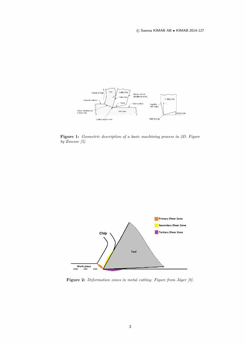
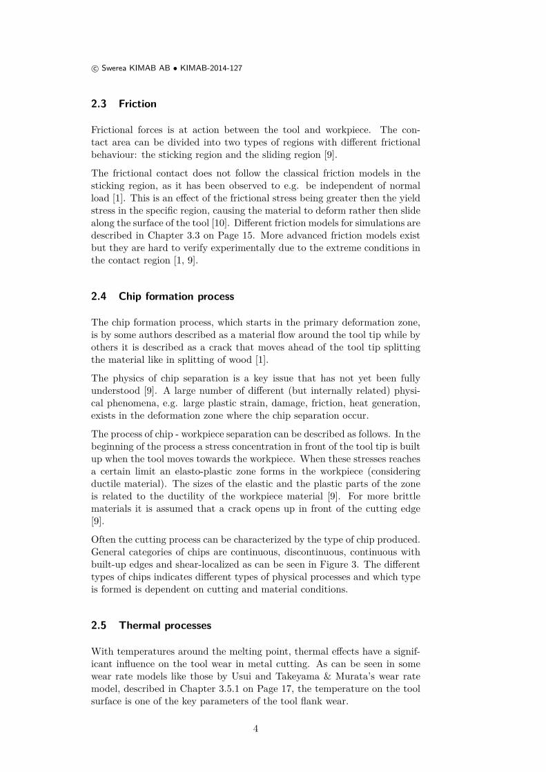
Figure 1 visualizes the geometry of the process of orthogonal cutting in twodimensions. It can be seen that the cutting tool has two sides, the rake faceand the flank face. The rake face where the chip is formed is situated at anangle, called rake angle, relative the normal of the new surface. The flankforms a relief angle (or clearance angle) to the new surface. The difference inheight between the original surface and the new surface is called the cuttingdepth.

2.2 Deformation zones

The chip formation is restricted to three main deformation zones, also calledshear zones, which can be seen in Figure 2, called the primary, secondary andtertiary deformation zones. In the primary deformation zone the workpiecematerial is forced to a quick change in direction under severe shear plasticstraining [1]. In the secondary deformation zone, situated along the rakeface of the tool, plastic deformation as well as friction is occurring and bothof them are producing heat [6]. In the tertiary deformation-zone there existsshearing due to surface friction [7].

2


Figure 1: Geometric description of a basic machining process in 2D. Figureby Emesee [5].

Figure 2: Deformation zones in metal cutting. Figure from Jäger [8].

3


2.3 Friction

Frictional forces is at action between the tool and workpiece. The con-tact area can be divided into two types of regions with different frictionalbehaviour: the sticking region and the sliding region [9].

The frictional contact does not follow the classical friction models in thesticking region, as it has been observed to e.g. be independent of normalload [1]. This is an effect of the frictional stress being greater then the yieldstress in the specific region, causing the material to deform rather then slidealong the surface of the tool [10]. Different friction models for simulations aredescribed in Chapter 3.3 on Page 15. More advanced friction models existbut they are hard to verify experimentally due to the extreme conditions inthe contact region [1, 9].

2.4 Chip formation process

The chip formation process, which starts in the primary deformation zone,is by some authors described as a material flow around the tool tip while byothers it is described as a crack that moves ahead of the tool tip splittingthe material like in splitting of wood [1].

The physics of chip separation is a key issue that has not yet been fullyunderstood [9]. A large number of different (but internally related) physi-cal phenomena, e.g. large plastic strain, damage, friction, heat generation,exists in the deformation zone where the chip separation occur.

The process of chip - workpiece separation can be described as follows. In thebeginning of the process a stress concentration in front of the tool tip is builtup when the tool moves towards the workpiece. When these stresses reachesa certain limit an elasto-plastic zone forms in the workpiece (consideringductile material). The sizes of the elastic and the plastic parts of the zoneis related to the ductility of the workpiece material [9]. For more brittlematerials it is assumed that a crack opens up in front of the cutting edge[9].

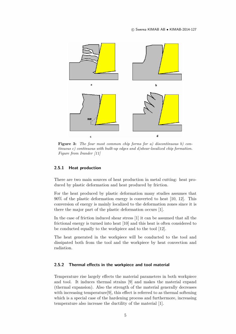
Often the cutting process can be characterized by the type of chip produced.General categories of chips are continuous, discontinuous, continuous withbuilt-up edges and shear-localized as can be seen in Figure 3. The differenttypes of chips indicates different types of physical processes and which typeis formed is dependent on cutting and material conditions.

2.5 Thermal processes

With temperatures around the melting point, thermal effects have a signif-icant influence on the tool wear in metal cutting. As can be seen in somewear rate models like those by Usui and Takeyama & Murata’s wear ratemodel, described in Chapter 3.5.1 on Page 17, the temperature on the toolsurface is one of the key parameters of the tool flank wear.

4


Figure 3: The four most common chip forms for a) discontinuous b) con-tinuous c) continuous with built-up edges and d)shear-localized chip formation.Figure from Irander [11]

2.5.1 Heat production

There are two main sources of heat production in metal cutting: heat pro-duced by plastic deformation and heat produced by friction.

For the heat produced by plastic deformation many studies assumes that90% of the plastic deformation energy is converted to heat [10, 12]. Thisconversion of energy is mainly localized to the deformation zones since it isthere the major part of the plastic deformation occurs [1].

In the case of friction induced shear stress [1] it can be assumed that all thefrictional energy is turned into heat [10] and this heat is often considered tobe conducted equally to the workpiece and to the tool [12].

The heat generated in the workpiece will be conducted to the tool anddissipated both from the tool and the workpiece by heat convection andradiation.

2.5.2 Thermal effects in the workpiece and tool material

Temperature rise largely effects the material parameters in both workpieceand tool. It induces thermal strains [9] and makes the material expand(thermal expansion). Also the strength of the material generally decreaseswith increasing temperature[9], this effect is referred to as thermal softeningwhich is a special case of the hardening process and furthermore, increasingtemperature also increase the ductility of the material [1].

5


2.6 Tool wear

Tool wear has a major influence of the economy of the machining operations.Process conditions chosen to optimize economy or productivity often resultin a tool life measured in minutes [13]. Thus, improvements in the under-standing and prediction of tool wear in metal cutting are very important.The tool wear also effects the chip formation and the residual stresses in thenew cut surface.For optimizations of the cutting processes in order to increase the tool life,tool life models such as the famous Taylor’s equation with extension, thatstates relations between tool-life and process parameters e.g. cutting speedcan be used [12]. In this work, the focus is on tool wear i.e. how and withwhich rate the tool gets worn down depending on cutting process variablessuch as normal stress and contact temperature [12]. Why models relatingcutting process variables with tool wear is of more interest than tool lifemodels.

2.6.1 Tool wear mechanisms

Tool wear in metal cutting can be described as a combination of severaldifferent mechanisms [14]. They can be grouped according to when theyact: abrasive and adhesive wear are dominant at lower cutting speeds whiletemperature-activated wear controls the wear as the cutting speed is in-creased. Diffusion wear, oxidation wear, and chemical wear are examples oftemperature-activated wear which is a function of the chemical compatibil-ity of the tool material and the workpiece material [15]. (Abrasive wear isthe main focus in this study since this is the mechanism that mainly drivesthe flank wear.)Abrasive wear is when hard particles in the workpiece material removestool material from the tool by mechanical action. The hard particles areeither fragments of the tool material removed at an earlier stage or hardparticles of the workpiece material [14]. Abrasive wear occurs mainly on theflank face but it effects both the flank face and rake face [15].Adhesive wear or attritional wear is a process of small particles from thetool being removed since they have welded or sicked to the chip surface dueto friction. In most cases adhesive wear rates are quite low except for cuttingof soft work materials under low speed and drilling [15].

2.6.2 Types of tool wear

There are two types of tool wear, defined by which area of the tool theyaffect.Crater wear produces wear by the form of small craters on the rake face[13]. Low levels of crater wear does not shorten the tool life but severe craterwear, usually induced by temperature-activated wear mechanisms, do [15].Flank wear occurs on the flank face (also called relief face) and is mainlydriven by the mechanism of abrasive wear. It forms wear lands which, when

6


rubbing the new formed machined surface, damages the surface and producelarge flank forces [15].

3 Finite Element Simulation of metal cutting

Finite Element, FE, simulations of metal cutting is a widely used and ap-preciated tool in product development of cutting tools. The simulations hasmany advantages: it is relatively quick, relatively cheap and can sometimesshow results and processes that are not yet possible to achieve experimen-tally due to the extreme conditions in the cutting zone. But FE simulationsof metal cutting also has certain limitations. Among them is to find a re-alistic way to model the chip - workpiece separation, to handle the largedeformations, to model the friction and to model the heat transfer.

3.1 Arbitrary Lagrangian-Eulerian adaptive meshing

A large problem when simulating machining with the finite element methodis that the mesh gets widely distorted which causes the simulations toabort. To handle this problem it is common to use the adaptive arbitraryLagrangian-Eulerian formulation of the mesh.

In Finite Element methods there are two common classical mathematicalformulations for describing motion: the Lagrangian description, where themesh moves with the material, and the Eulerian description, where the meshis fixed in space and the material moves with respect to the grid.

In the Lagrangian description, which is the most widely used method whensimulating problems in solid mechanics, the displacement vector is a func-tion of the material particles original position. In the Eulerian description,which is the standard method in Computational Fluid Dynamics (CFD) thedisplacement is expressed i terms of the current coordinates [16]. Both ofthe methods have their advantages and disadvantages, among them is thatthe Lagrangian descriptions, without frequent remeshing, lack the ability tofollow large deformations something that the Eulerian approach does witha relative ease [17]. A main shortcomings of the Eulerian description is thatthe material flow needs to be defined prior to the simulations [6].

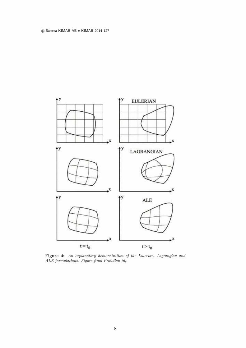
In the Arbitrary Lagrangian-Eulerian description (ALE), which is a com-bination of the Lagrangian description and the Eulerian description, themesh is allowed to move in an arbitrarily specified way. For an explanatorydemonstration of the differences between Eulerian, Lagrangian and ALE de-scriptions see Figure 4. In this work an adaptive mesh approach with theALE formulation is treated.

The ALE adaptive meshing is a single mesh method. This means that thepositions of the nodes in the original mesh is corrected by means of a certainalgorithm rather than that a new mesh is imposed. There are two main stepsin the ALE adaptive meshing, relocation of the nodes to create the reformedmesh (the so called mesh-update procedure described in Chapter 3.1.2) and

7


Figure 4: An explanatory demonstration of the Eulerian, Lagrangian andALE formulations. Figure from Proudian [6].

8


remapping of the solution variables to this reformed mesh (the so calledstress-update procedure described in Chapter 3.1.4).

3.1.1 Boundaries in ALE methods

The ALE method can be applied to a wide range of problems by definingthe movement of the mesh and the form of the boundaries. There are twoprimary types of boundaries for ALE domains, Eulerian and Lagrangianboundaries, with the main difference that the material points are allowedto flow across Eulerian boundaries while across Lagrangian boundaries theyare not.

At a Lagrangian boundary the nodes follows the material in the directionnormal to the boundary making the mesh cover the same material domainduring the entire analysis.

3.1.2 Mesh-update procedures

The mesh-update procedure is defined by several different algorithms andchoices e.g. the remeshing criteria - which nodes to move and when, smooth-ing algorithms and geometric aspects such as: geometric enhancement andcurvature refinement.

ALE adaptive meshing is not performed equally over the entire mesh butserves to reshape the mesh where necessary. The ALE adaptive mesh algo-rithm in ABAQUS always strives to reduce element distortion by improvingelement aspect ratio (i.e. to get all sides of the element to be of the samelength) sometimes under the option to preserve initial mesh gradation [2].

There are several algorithms for relocating the nodes to the new mesh.In ABAQUS/Explicit there are two quite basic options, either a volume-weighted average of the element centres or an average of the positions of theadjacent nodes connected by an element edge. A more complicated smooth-ing algorithm is based on a higher-order average of the eight (in the 2D case)nearest nodes.

In ABAQUS/Explicit there is an extra choice for the mesh-update proce-dure called curvature refinement. The functionality of this is to "pull moreelements into areas of high curvature" [2].

The remeshing criteria in ABAQUS is not based on an error function butsimply stated as a frequency telling how often the mesh is to be updated.Another parameter stated is the number of iterations for the relocationof the nodes. In ABAQUS/Explicit these iterations, which are performedaccording to chosen smoothing algorithm, are called mesh sweeps. Themesh sweeps can be based either on the current nodal position (often usedfor Lagrangian problems) or on the nodal position in the end of the previousadaptive mesh increment (recommended for Eulerian problems) [2].

9


3.1.3 Motion in ALE

The ALE conservation equations are very similar to the Eulerian conserva-tion equations and the ALE description is therefore sometimes called quasiEulerian description [17]. In both the Eulerian and the ALE descriptionsthere are advective effects due to relative motion between the material andthe grid. These advection terms, which are not a part of the classical La-grangian equations, rises a need for an, from the Lagrangian point of view,extended solution algorithm [17]. This extension of the solution algorithmis the so called stress-update procedure.

3.1.4 Stress-update procedures

The conservation equations can be handled in several different ways, whichcan be classified into two different categories: split and unsplit methods [17].In an unsplit method the non symmetric system of equations is solved di-rectly [2, 17]. A split method decouples the calculations into two differentphases: a Lagrangian (material) phase, for calculations of the material as-pects, and a transport phase, for calculations of the advective terms [2, 17].The main advantage of using a split method is its computational efficiencybut choosing a split method comes at the cost of losing accuracy. For explicitapproaches this loss is within acceptable limits since the time increment issufficiently small.In the Lagrangian phase the advective effects are neglected and hence thecalculations exactly follows the procedure for purely Lagrangian descriptions[17]. It should be noted that it is common to let the Lagrangian phase beexecuted in the mesh-update loop and then perform the calculations of thetransport phase only after the mesh has been updated [17].In the transport phase the advective effects, in form of hyperbolic partialdifferential equations, has to be accounted for. The solutions of these equa-tions represent spatial travelling waves, giving them a spatial movementdirection. For the calculations in the transport phase an upwind scheme isused, taking this directionality into account [18]. ABAQUS/Explicit offersthe possibility to chose between a first- and a second-order scheme, althoughthe first order scheme is not recommended due to its major disadvantage ofdiffusing sharp gradients over time[2, 18] .

3.2 Chip - workpiece separation in an FE environment

A big challenge when creating an FE model of machining is to get thematerial separation in the cutting zone to behave like it does in reality. Thephysical processes of chip - workpiece separation depends on several differentparameters, in relations not yet determined and depending on material andcutting conditions. The effects of the limited knowledge of the real worldbehaviour tend to give the models a sense of arbitrariness.The challenge has historically been handled with a path dependent partingcriteria. During the last decade other techniques such as: multiple remesh-

10


Separation algorithm Advantages Disadvantages

Adaptive meshing No non-physicalcriteria needed

Computationallyheavy

Previously definedparting line

Easy to control theseparation

Completelynon-physical

Damage and failurecriteria

Can be related tophysical parameters

Element deletion givesrise to loss of mass

Meshless/meshfreemethods

No non-physicalcriteria needed

Not as exact as FEM

ALE- with Eulerianboundaries

No non-physicalcriteria needed

Predefined chipformation needed

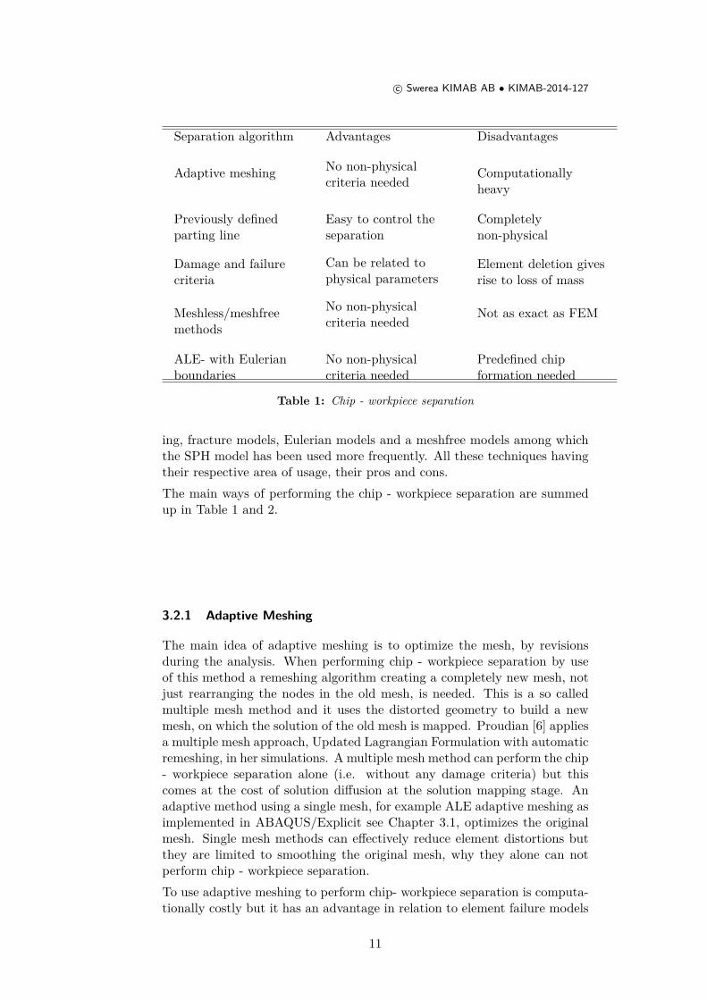
Table 1: Chip - workpiece separation

ing, fracture models, Eulerian models and a meshfree models among whichthe SPH model has been used more frequently. All these techniques havingtheir respective area of usage, their pros and cons.The main ways of performing the chip - workpiece separation are summedup in Table 1 and 2.

3.2.1 Adaptive Meshing

The main idea of adaptive meshing is to optimize the mesh, by revisionsduring the analysis. When performing chip - workpiece separation by useof this method a remeshing algorithm creating a completely new mesh, notjust rearranging the nodes in the old mesh, is needed. This is a so calledmultiple mesh method and it uses the distorted geometry to build a newmesh, on which the solution of the old mesh is mapped. Proudian [6] appliesa multiple mesh approach, Updated Lagrangian Formulation with automaticremeshing, in her simulations. A multiple mesh method can perform the chip- workpiece separation alone (i.e. without any damage criteria) but thiscomes at the cost of solution diffusion at the solution mapping stage. Anadaptive method using a single mesh, for example ALE adaptive meshing asimplemented in ABAQUS/Explicit see Chapter 3.1, optimizes the originalmesh. Single mesh methods can effectively reduce element distortions butthey are limited to smoothing the original mesh, why they alone can notperform chip - workpiece separation.To use adaptive meshing to perform chip- workpiece separation is computa-tionally costly but it has an advantage in relation to element failure models

11


Separation algorithm Steady / Unsteadystate model

Good for modeling

Adaptive meshing Unsteady Residual stresses

Chip formation

Cutting forces

Previously definedparting line Unsteady -

Damage and failurecriteria

Unsteady Chip formation

Meshless/meshfreemethods

Unsteady Chip formation

Cutting forces

The metal dead zonefor cutting withstrongly worn tools

Eulerian model SteadyTemperaturedistribution in steadystate machining

Table 2: Chip - workpiece separation

12


since no material is removed and no non-physically criteria is used. As men-tioned above the solution is a bit diffused every time the solution is mappedto the new mesh making the solutions a bit less accurate.

3.2.2 Element failure models

Modeling chip - workpiece separation with element failure models in FEMmeans setting a condition, based on a value for a certain parameter or acombination of parameters, for when the material breaks. The failure is abinary parameter of the element with the value one before failure and zerowhen failed. After failure the element is deleted from the mesh exposing theneighbouring elements.

Element failure is probably the most common way of performing chip -workpiece separation today. In relation to adaptive remeshing and Eulerianmodels, element failure reduces the computational cost. Today many quitephysically realistic damage and failure criterion has been proposed. Amongthem the Johnson-Cook damage law (presented in Chapter 4.3.4) seems togive good results.

The main disadvantage with element failure is the deletion of material. Itis generally non-physical that mass is removed from the process and thisremoval effects the forces (pressure) between the tool and workpiece andthereby it effects all the results of the simulations. To reduce these effectsthe mesh density has to be very fine, leading to reduced efficiency gain inrelation to frequent remeshing. A discussion about whether the materialactually breaks in the cutting zone or not can be held. For the formationof segmented chips it might be necessary with a damage criteria but that isa breakage occurring at the top of the workpiece while the chip - workpieceseparation occurs in the surrounding of the nose of the cutting tool.

3.2.3 SPH simulation of metal cutting

In several studies a meshfree, smooth particle hydrodynamics (SPH) modelfor simulations of metal cutting is used [19, 20, 21, 22, 23]. The SPHmethod handles the large deformations that occurs during cutting simu-lations through a loss of cohesion between the particles [22].

Despite its name, to say that the SPH method is a particle method is not re-ally correct. A particle method incorporates particle equations but the SPHmethod is just another way to discretize the continuum equations [2]. Onecould say that SPH is a meshfree FEM method. When the FEM discretizesthe material in finite elements built-up by nodes, with arrangements statedin the connectivity matrix, SPH discretizes the material particles which canbe thought of as single node elements with their internal ordering not de-termined by a connectivity matrix.

Instead of assuming connectivity between nodes to build the spatial deriva-tives, as is the case in FEM, the SPH uses a kernel approximation to calculatespatial derivatives [23]. The particle approximation is given by:

13


h∏f(x) =

∫f(y)W (x− y, h) dy (1)

where h is the smoothing length, and W is the centrally peaked kernelfunction (often a cubic spline , which for example is default in ABAQUS[2]).

When using the SPH method for chip - workpiece separation in cutting sim-ulations no non-physical separation criterion is needed and no remeshing isneeded to handle the mesh distortions. In general the SPH method is lessaccurate then Lagrangian FEM and ALE FEM, and it is therefore recom-mended only for applications where the deformation is so severe that onlySPH is possible. Since this is the case for machine cutting it is an accept-able method. An advantage with SPH compared to FEM is an increasedtransparency in the assumptions made [20].

For analyses of cutting with strongly worn tools the SPH method has shownto be able to represent the metal dead zone which is a physical phenomenaearlier observed in experiments [21, 23], which can explain the increased feedforce when cutting with worn tools.

For predicting chip formation and cutting forces the SPH method gives goodcorrelation with experiments and FE simulations [22, 21, 20, 19].

Other meshfree/meshless methods have been tried in some studies like theElement-free Galerkin Method (EFGM) and the Finite Pointset Method(FPM), but the SPH method is by far the most common one within manu-facturing technology [24].

3.2.4 Eulerian models

An Eulerian model of chip - workpiece separation simulates the materialflow around the tool-tip, without any non-physically cutting conditions, forsteady state machining. Due to the nature of the Eulerian mesh, see Chap-ter 3.1, this type of model requires a predefined chip geometry, making itunusable for modeling chip formation.

An option is to model the chip formation part of the problem with anotherchip - workpiece separation model or using an experimentally determinedgeometry to get the form of the chip and than use the Eulerian model forcalculating cutting forces, residual stresses and tool wear.

3.2.5 Path dependent parting

When using path dependent parting a cutting line is defined beforehand,usually it is the line from the tool tip and forward. Along this line a sepa-ration indicator criterion, based on either geometrical or physical consider-ations, is calculated and the elements reaching the criteria are deleted (orunhooked if using cohesive elements). A possible geometrical indicator is a

14


critical distance between the tool tip and the nearest node along a predefinedline.

Path dependent parting was a lot more common during the 80:s and 90:s thenit is today. With the path dependent parting a crack leaping ahead of thetool-tip is unavoidable. This crack was till not to long ago considered to bein harmony with the theories about real world machining, but recent yearsthis has been reconsidered. Today path dependent parting is concideredcompletly unphysical. But there are, of course, also advantages with thismethod. When using it, the chip separation is easy to control and since thecutting line is known in advance the elements can be made very small thereand thus reducing the element deletion effects on the simulation.

3.3 Friction models

The choice of friction model has a major impact on the predicted tool wearsince it affects both the heat produced in the contact region and the normalstresses between the tool and the workpiece.

Several different models for the frictional behaviour between the tool andthe workpiece has been proposed, a few of them are described below. Itis important to note that the mechanisms behind the problem of frictionare not yet completely understood [10] and the choice of friction model istherefore often driven by a wish for simplicity.

3.3.1 Coulomb friction model

The Coulomb friction model is the most simple and classical of the fric-tion models. It is basically an implementation of the Coulomb’s law. TheCoulomb friction model states, as can be seen in Equation (2), that the fric-tional stress τf is proportional to the normal stress σn times the constantfrictional coefficient µ.

τf = µσn (2)

The Coulomb friction model was used for simulations of residual stress byProudian [6] in her thesis at KTH in 2012. It has also been used by Arrazolaet al. [25] and by Issa et al. [26] but then with a friction coefficient dependingon temperature and sliding velocity at the contact interfaces.

3.3.2 Constant shear model

The constant shear model assumes the frictional stress τf to be constant,and defined as:

τf = mτY (3)

where τY is the yield shear stress of the material, defined [2, 10] as τY =σY /√

3, and m is the friction factor [6].

15


3.3.3 Sticking zone and sliding zone model

A common friction model for simulations of metal cutting is the stick-slipmodel defining a sticking region around the tool tip and a sliding regionon all other areas subjected to contact. For simulation purpose it can beimplemented as follows [10, 27],

τf (x) = µσn µσn < τY (4)τf (x) = τY µσn ≥ τY (5)

where Equation (4) and (5) describes a case where the Coulomb frictionmodel is used up to a certain level of shear stress and for normal stressesabove that value a constant shear model is used. Please note the similaritybetween Equation (4) and (2) and Equation (5) and (3).

3.3.4 Friction in smooth particle hydrodynamic simulations

In some studies of smooth particle hydrodynamic, SPH, simulations of metalcutting both the workpiece and the tool has been modelled with SPH par-ticles. This opens up for the possibility to let go of the applied frictioncondition and just use contact between two SPH surfaces. This method hasshown to give really good results which sometimes can explain which con-tact conditions should be applied in FE simulations [23]. It should be notedthat the SPH friction still needs to be validated before it can be considereda reliable tool in the prediction of cutting behaviour.

3.4 Heat transfer models

With temperature differences of 500 ◦C - 1400 ◦C [4], the temperature has alarge impact on the accuracy of the machining simulation. The heat transferdepends on the cutting velocity, the material of the tool and the workpiece.In real world cutting sometimes cutting fluids are used as coolants, whichfurther increases the complexity in the heat transfer models.

3.4.1 Adiabatic assumption

Sometimes orthogonal cutting is modelled as an adiabatic process, i.e. asif no heat transfer occurs. This can be assumed when the cutting speed ishigh and when the material points studied are not in the tool but in theworkpiece [23, 9, 1].

An adiabatic FE simulation means having no heat transfer between theelements. A way to implement this is to set the heat conduction matrix tozero [9].

16


3.4.2 Coupled Thermal-Stress analysis

In the physical world cutting is a thermally-mechanically coupled problemand some of the heat produced close to the workpiece surface is conductedto the tool. In many cases the heat transferred to the tool is considered tobe around 10% of the heat produced in the workpiece near the tool.The conductive heat transfer between the tool and the workpiece is oftenconsidered to be linear and is then defined as:

q = h(θA − θB) (6)

where q is the heat flux per unit area crossing the interface from point A onthe workpiece surface to point B on the tool surface, h is the heat conductioncoefficient, θA is the workpiece temperature and θB is the tool temperature.According to some authors the heat conduction coefficient is a constant [14]while according to others it depends on the contact pressure [10, 28].

3.5 FE models of tool wear

The tool wear models describe a rate of local volume loss on the tool face, perunit time, per unit area [28]. In FE simulations these models are often usedin a simulation cycle where the tool wear is calculated in a step separatedfrom the FE simulation and thereafter used in further simulation steps.

3.5.1 Tool wear rate models

Uisui et al. [29] derived a wear rate model based on the equation ofadhesive wear, which has shown to be adequate for both flank and craterwear of tungsten carbide tools [28].

∂W

∂t= Avsσnexp(−

B

T) (7)

where ∂W∂t is the rate of volume loss on the tool contact face per unit area per

unit time, vs is the sliding velocity at the contact surface, σn is the normalstress, T is the temperature measured i Kelvin and A and B are constants.Takeyama and Murata, as cited in [28], proposed a wear rate equation(see Equation (8)) by considering abrasive wear and diffusive wear.

∂W

∂t= G(V, f) +Dexp(− E

RT) (8)

here the first term G(V, f) is the abrasive wear in which; G is a constant,V is the cutting speed and f is the feed rate and the second term is thediffusive wear in which; D is a constant, E is the process activation energyand R is the universal gas constant [30].

17


3.5.2 Cyclic implementation

FE simulations of tool wear are often implemented as a cyclic system [12,30] with three distinctive steps [31]. Here the Usui’s wear rate model, seeEquation (7), are used since it is common in literature, gives satisfactoryresults and the values of the parameters are easily achieved from the FEsimulation.Chip formation The parameters T , vs and σn are calculated in the FEcutting simulation for nodes on the tool surface that are in contact with theworkpieceWear rate calculation A wear rate based on Usui’s wear rate model iscalculated from the values for T , vs and σn given from the previous step.This calculation is often performed in a user subroutine [31].Tool geometry update Based on the tool wear rate the nodes on thetool surface is moved in a tool wear direction which is calculated differentlydepending on the nodes position and method chosen See for example [31, 12].

4 Material models

In metal cutting the material undergoes rapid elasto-plastic deformation un-der extreme conditions. To give an adequate result the material model mustbe able to describe deformation behavior such as hardening and softeningover a great ranges of strain, strain rate and temperature [1].

4.1 Hardening

For many materials the stress after initial yielding keep increasing with in-creasing strain. This phenomena is called strain hardening [32]. For mate-rial subjected not only to increasing strain after yielding but also to reversedloading, two extreme cases of behavior can be defined: isotropic and kine-matic hardening. Hardening can also depend on other parameters, such astemperature and plastic strain rate.While the hardening rules effects the size and location of the yield surface,the yield criterion defines the shape.

4.1.1 Yield criterion

There are several different yield criteria. Among them the von Mises yieldcriterion is the most common and it is specially suited for metals since formost metals all volumetric response is linear elastic [16]. Therefor only thevon Mises yield criterion is treated and used in this work.The von Mises condition reads:

f(σij) = (32sklskl)

1/2 − σy = 0 (9)

18


where skl is the deviatoric stress tensor and σy is the yield stress, which canbe a material constant or the isotropic hardening component (see Chapter4.1.3). Equation (9) describes a cylinder with circular cross section andradius

√23σy in stress space.

The von Mises condition for mixed or kinematic hardening reads:

f(σij) =[3

2(skl − αkl)(skl − αkl)]1/2− σy = 0 (10)

where αkl is the back stress tensor (see Chapter 4.1.4) defining the centerof the circular cross section of the yield stress in stress space. If αkl = 0Equation (10) reduces to the initial von Mises criterion, i.e. Equation (9).

4.1.2 Flow rule

The associated flow rule for isotropic hardening is given by:

εplij = ˙εpl ∂f∂σij

= ˙εpl 3skl2σy(11)

where ˙εpl = (32 εplij ε

plij)1/2 is the equivalent plastic strain rate. The associated

flow rule for kinematic or mixed hardening is given by:

εplij = ˙εpl ∂f∂σij

= ˙εpl 3(skl − αkl)2σy

(12)

4.1.3 Isotropic hardening

Isotropic hardening describes a process where the elastic region in the stressspace expands with increasing effective plastic strain. This means that theyield surface is represented by a circle (considering a von Mieses material)with a radius depending on the effective plastic strain [32].

For isotropic hardening processes the yield stress is given by:

σy = σy0 +K(εpl, ˙εpl, T ) (13)

where σy0 is a constant initial yield stress and K(εpl, ˙εpl, T ) can be modeledin several different ways, most common as a linear function K(εpl) = H ˙εplor as a power law K(εpl) = h( ˙εpl)a where H, h and a are material constants[32].

19


4.1.4 Kinematic hardening

Opposed to isotropic hardening, the elastic region is invariable in a processof kinematic hardening. Instead it can be visualized as if the center pointof the yield surface translates (see Equation (10)) in the stress space by aback stress vector which depends on the effective plastic strain [32]. Theobservation of kinematic hardening is sometimes called Bauschinger effect[16].There are many possible choices for modeling evolution of the back stressα. A classical model is the Melan-Prager’s evolution law [16] which reads:

αij = cεplij (14)

where c is a material parameter. Another evolution law, proposed by Arm-strong and Frederick [16] is

αij = c

(23 ε

plij −

αijα∞

˙εpl)

= C1σy

(sij − αij) ˙εpl − γαij ˙εpl (15)

where α∞, C and γ are material parameters and the equivalent plastic strainrate is given by the flow rule for kinematic hardening, see Equation (10).Note that if α∞ goes to infinity then γ goes to zero and the Armstrong-Frederick evolution law in Equation (15) reduces to the Melan-Prager’s evo-lution law in Equation (14).The Armstrong-Frederick model was generalized by Chaboche [16] by su-perposing several Armstrong-Frederick terms after each other

αij =∑k

αkij (16)

αkij = Ck1σy

(σij − αkij) ˙εpl − γkαkij ˙εpl (17)

where k is the number of back stresses and Ck and γk is the Chabochematerial parameters.

4.2 The Johnson-Cook model

The Johnson-Cook constitutive material model, which is in implementa-tion of isotropic hardening, is a common material model for describing thethermo-visco-plastic behavior of the workpiece in a cutting process [4]. Toattain the data for deriving the material parameters, torsion tests over wideranges of strain rates, static tensile tests, dynamic Hopkinson bar tensiletests and Hopkinson bar tests are performed [6].The flow stress is formulated as a function of strain, strain-rate and tem-perature as can be seen in Equation (18).The Johnson-Cook equation reads:

σ = (A+B(εpl)n)[1 + Cln

˙εpl

ε0

](1− θm

)(18)

20


where σ is the equivalent flow stress, A is the initial yield strength of thematerial, εpl is the equivalent plastic strain and ˙εpl is the equivalent plasticstrain rate which is normalized with a reference strain rate ε0. The param-eters B, n, C and m are material model parameters. θ is the homologustemperature given in Equation (19).

θ = (θ − θroom)(θmelt − θroom) (19)

here θ is the instantaneous temperature of the workpiece, θroom is the roomtemperature and θmelt is the material melting temperature.The Johnson-Cook model can be seen as a multiplication of three distinctiveterms

σ = f(ε)g( ˙εpl)h(θ) (20)

where

f(ε) = A+B(εpl)n (21)

g( ˙εpl) = 1 + Cln˙εpl

ε0(22)

h(θ) = 1−( θ − θroomθmelt − θroom

)m(23)

Equation (21) describes an isotropic strain hardening behavior, Equation(22) describes strain rate sensitivity and Equation (23) describes a thermalsoftening behavior [33].

The Johnson-Cook model has been criticized for neglecting the couplingeffects of strain, strain rate and temperature [33]. It also lacks ability tocapture some important behavior during high strain and high strain rate (forexample flow softening) [33], a very important comment in the environmentof cutting since the simulations are then including strain rates up to 106 andstrains up to 10 [1].

4.3 Damage and failure models

There are two different types of damage models in ABAQUS, dynamic dam-age and progressive damage. The main difference between them is that thematerials load carrying capacity is reduced progressively after a certain cri-teria is met in the progressive damage while it is changed discretely when thedynamic damage parameter has reached a critical value for dynamic dam-age. ABAQUS recommends the later one to be used only for high strainrate dynamic problems [2].

21


Considering e.g. metals under tension, the FE model of progressive damageis based on the assumption that the material, after a linear elastic phase anda plastic yielding phase, reaches a phase of strain softening. In the strainsoftening phase, which starts at a damage initiation point, the materialundergoes a reduction of load carrying capacity, i.e. a damage evolutionphase, before a final failure [2].In the dynamic damage model the material undergoes the linear elastic phaseand the plastic yielding phase with stress strain curves just as for the modelwith progressive damage. But instead of damage initiation and evolution theelement just fails when the damage criteria is met at all integration pointsin the element.There are several possible choices for the damage initiation criteria, e.g.Ductile damage (see Chapter 4.3.1) and Shear damage (see Chapter 4.3.2)as described below, and damage evolution criteria (see Chapter 4.3.3) inABAQUS/Explicit. For elements where the material has reached failure,i.e. when it no longer has any load carrying capacity, a deletion criteria canbe imposed. This means that failed elements are deleted from the simulation.For further discussion on effects of element removal see Chapter 3.2.2.

4.3.1 Progressive ductile damage initiation

In the ductile damage initiation criterion the critical equivalent plastic strain,εplD, is a function of stress triaxiality, η, and plastic strain rate, ˙εpl, i.e.εplD(η, ˙εpl). The onset of damage is met when the following criterion is satis-fied:

ωD =∫ 1εplD(η, ˙εpl)

dεpl = 1 (24)

where ωD is a monotonically increasing state variable. The model of ductiledamage is based on phenomenological observations of damage related tovoids in the material [2]. The ductile damage initiation criterion is specifiedas a table with εplD(η, ˙εpl).

4.3.2 Progressive Shear damage

The shear damage initiation criterion assumes that the critical equivalentplastic strain, εplS , depends on shear stress ratio, θS , and plastic strain rate,˙εpl. With the shear stress ratio defined as:

θS = (q + ksp)τmax

(25)

where q is the Mises equivalent stress, p is the pressure stress, τmax isthe maximum shear stress and ks is a material parameter. We then haveεplS (θs, ˙εpl). The onset of damage is met when the following criterion is sat-isfied:

22


ωS =∫ 1εplS (θS , ˙εpl)

dεpl = 1 (26)

where ωS is a monotonically increasing state variable. The model of sheardamage is based on phenomenological observations of damage related toshear bands in the material [2]. The shear damage initiation criterion isspecified as a table with εplS (θS , ˙εpl).

4.3.3 Progressive damage evolution

The damage evolution defines the material behavior after damage initiation.The stress in the material is in this phase given by:

σ = (1−D)σ (27)

where σ is the undamaged stress, i.e. the stress that would exist in thematerial in absence of damage, and D is the damage variable which is zeroat damage initiation and one at complete failure. This is a softening ofthe material, a reduction in material stiffness. If there are several differentfailure mechanisms active, ABAQUS calculates a damage evolution thattakes them all into account [2].

4.3.4 Cumulative Johnson-Cook damage

This model is a dynamic shear failure model in ABAQUS/Explicit which isused for the chip - workpiece separation in orthogonal cutting simulationsby Agmell et al.[10] and Zouhar et al. [34].For the shear failure model, failure occurs when the damage parameter ωdefined by Equation (28) reaches the value one.

ω = εpl0 +∑

∆εpl

εplf(28)

where εpl0 is the initial value of the equivalent plastic strain, ∆εpl is anincrement of the equivalent plastic strain and εplf is the critical strain atfailure. The summation is performed over all steps of the analysis.For the Johnson-Cook damage law the strain at failure is given by:

εplf =[D1 +D2 expD3( p

σ)][

1 +D4ln( εpl

ε0)][

1 +D5θ − θroom

θmelt − θroom

](29)

The element has failed when the shear failure criterion is met for the inte-gration point (since in this work only first order quadrilateral elements withreduced integration and first order triangular elements, both having onlyone integration point) in the element [2]. Then all the stress componentswill be set to zero and the element will be deleted from the simulation.

23


20NiCrMo5 AISI 4041

Density [kg/m3] 7800 7850Poisson’s ratio 0.3 0.29Youngs modulus [Pa] 2.1 · 1011 2.19 · 1011

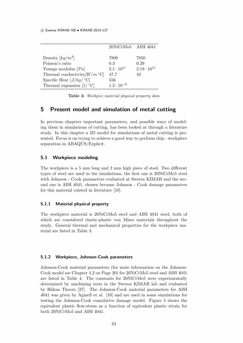
Thermal conductivity[W/m ◦C] 47.7 42Specific Heat [J/kg/ ◦C] 556Thermal expansion [1/ ◦C] 1.2 · 10−6

Table 3: Workpice material physical property data

5 Present model and simulation of metal cutting

In previous chapters important parameters, and possible ways of model-ing them in simulations of cutting, has been looked at through a literaturestudy. In this chapter a 2D model for simulations of metal cutting is pre-sented. Focus is on trying to achieve a good way to perform chip - workpieceseparation in ABAQUS/Explicit.

5.1 Workpiece modeling

The workpiece is a 5 mm long and 2 mm high piece of steel. Two differenttypes of steel are used in the simulations, the first one is 20NiCrMo5 steelwith Johnson - Cook parameters evaluated at Swerea KIMAB and the sec-ond one is AISI 4041, chosen because Johnson - Cook damage parametersfor this material existed in literature [10].

5.1.1 Material physical property

The workpiece material is 20NiCrMo5 steel and AISI 4041 steel, both ofwhich are considered elastic-plastic von Mises materials throughout thestudy. General thermal and mechanical properties for the workpiece ma-terial are listed in Table 3.

5.1.2 Workpiece, Johnson-Cook parameters

Johnson-Cook material parameters (for more information on the Johnson-Cook model see Chapter 4.2 on Page 20) for 20NiCrMo5 steel and AISI 4041are listed in Table 4. The constants for 20NiCrMo5 were experimentallydetermined by machining tests in the Swerea KIMAB lab and evaluatedby Håkan Thoors [27]. The Johnson-Cook material parameters for AISI4041 was given by Agmell et al. [10] and are used in some simulations fortesting the Johnson-Cook cumulative damage model. Figure 5 shows theequivalent plastic flow-stress as a function of equivalent plastic strain forboth 20NiCrMo5 and AISI 4041.

24


20NiCrMo5 AISI 4041

A [Pa] 4.9 · 108 5.95 · 108

B [Pa] 6 · 108 5.8 · 108

n 0.21 0.133C 0.015 0.023m 0.6 1.03ε0 1 1Tmelt [K] 1900 1850Troom [K] 300 300

Table 4: Johnson-Cook constitutive material model constants for 20NiCrMo5and AISI 4041

0 0.2 0.4 0.6 0.8 1

0.8

0.9

1

1.1

Equivalent plastic strain

Equivalent

plastic

flow

stress

[GPa]

20NiCrMo5AISI 4041

Figure 5: Johnson-Cook stress-strain curves for 20NiCrMo5 and AISI 4041,with T = Troom = 300K and ˙εpl = ε0 = 1

5.1.3 Implementation of kinematic hardening component

For trying out the possibilities with the SPH model, a material model withkinematic hardening is implemented. This implementation is written asa tabular data on the form of ABAQUS/Explicit built in function Com-bined Hardening, which takes in yield stress as a function of plastic strainand possibly temperature (although here the temperature dependency is ne-glected). The tabulated data is fitted to imitate the curves generated fromthe Johnson-Cook equation achieved with the parameter values from Table4.ABAQUS/Explicit then automatically finds the parameters for the Chabochemodel, see Chapter 4.1.4 on Page 20, for a given number of back stresses

25


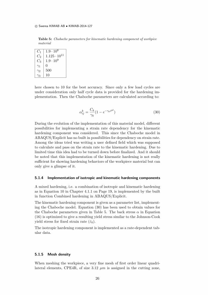
Table 5: Chaboche parameters for kinematic hardening component of workpicematerial

C1 1.9 · 108

C2 1.125 · 1011

C3 1.9 · 109

γ1 0γ2 500γ3 10

here chosen to 10 for the best accuracy. Since only a few load cycles areunder consideration only half cycle data is provided for the hardening im-plementation. Then the Chaboche parameters are calculated according to:

αkij = Ckγk

(1− e−γk εpl) (30)

During the evolution of the implementation of this material model, differentpossibilities for implementing a strain rate dependency for the kinematichardening component was considered. This since the Chaboche model inABAQUS/Explicit has no built in possibilities for dependency on strain rate.Among the ideas tried was writing a user defined field which was supposedto calculate and pass on the strain rate to the kinematic hardening. Due tolimited time this idea had to be turned down before finalized. And it shouldbe noted that this implementation of the kinematic hardening is not reallysufficient for showing hardening behaviors of the workpiece material but canonly give a glimpse of it.

5.1.4 Implementation of isotropic and kinematic hardening components

A mixed hardening, i.e. a combination of isotropic and kinematic hardeningas in Equation 10 in Chapter 4.1.1 on Page 19, is implemented by the builtin function Combined hardening in ABAQUS/Explicit.The kinematic hardening component is given as a parameter list, implement-ing the Chaboche model. Equation (30) has been used to obtain values forthe Chaboche parameters given in Table 5. The back stress α in Equation(16) is optimized to give a resulting yield stress similar to the Johnson-Cookyield stress for fixed strain rate (ε0).The isotropic hardening component is implemented as a rate-dependent tab-ular data.

5.1.5 Mesh density

When meshing the workpiece, a very fine mesh of first order linear quadri-lateral elements, CPE4R, of size 3.12 µm is assigned in the cutting zone,

26


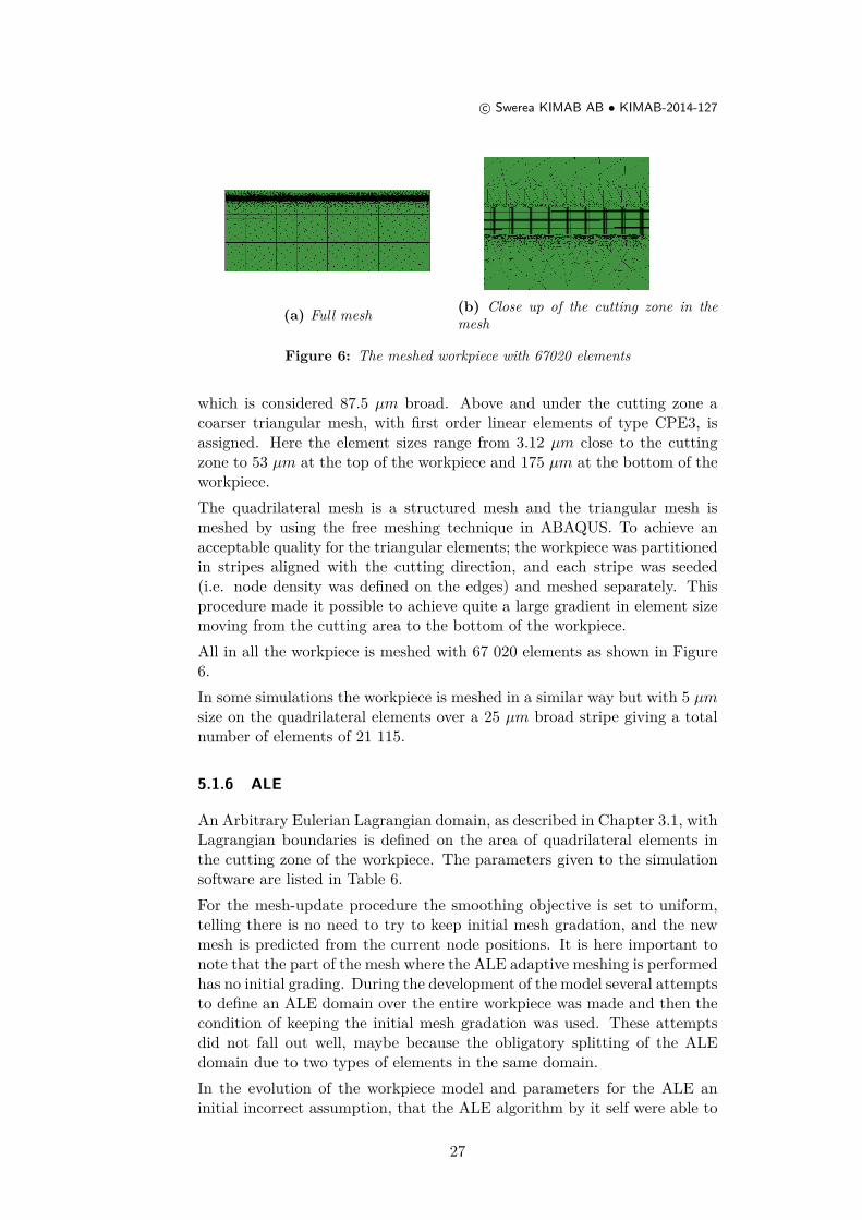
(a) Full mesh (b) Close up of the cutting zone in themesh

Figure 6: The meshed workpiece with 67020 elements

which is considered 87.5 µm broad. Above and under the cutting zone acoarser triangular mesh, with first order linear elements of type CPE3, isassigned. Here the element sizes range from 3.12 µm close to the cuttingzone to 53 µm at the top of the workpiece and 175 µm at the bottom of theworkpiece.The quadrilateral mesh is a structured mesh and the triangular mesh ismeshed by using the free meshing technique in ABAQUS. To achieve anacceptable quality for the triangular elements; the workpiece was partitionedin stripes aligned with the cutting direction, and each stripe was seeded(i.e. node density was defined on the edges) and meshed separately. Thisprocedure made it possible to achieve quite a large gradient in element sizemoving from the cutting area to the bottom of the workpiece.All in all the workpiece is meshed with 67 020 elements as shown in Figure6.In some simulations the workpiece is meshed in a similar way but with 5 µmsize on the quadrilateral elements over a 25 µm broad stripe giving a totalnumber of elements of 21 115.

5.1.6 ALE

An Arbitrary Eulerian Lagrangian domain, as described in Chapter 3.1, withLagrangian boundaries is defined on the area of quadrilateral elements inthe cutting zone of the workpiece. The parameters given to the simulationsoftware are listed in Table 6.For the mesh-update procedure the smoothing objective is set to uniform,telling there is no need to try to keep initial mesh gradation, and the newmesh is predicted from the current node positions. It is here important tonote that the part of the mesh where the ALE adaptive meshing is performedhas no initial grading. During the development of the model several attemptsto define an ALE domain over the entire workpiece was made and then thecondition of keeping the initial mesh gradation was used. These attemptsdid not fall out well, maybe because the obligatory splitting of the ALEdomain due to two types of elements in the same domain.In the evolution of the workpiece model and parameters for the ALE aninitial incorrect assumption, that the ALE algorithm by it self were able to

27


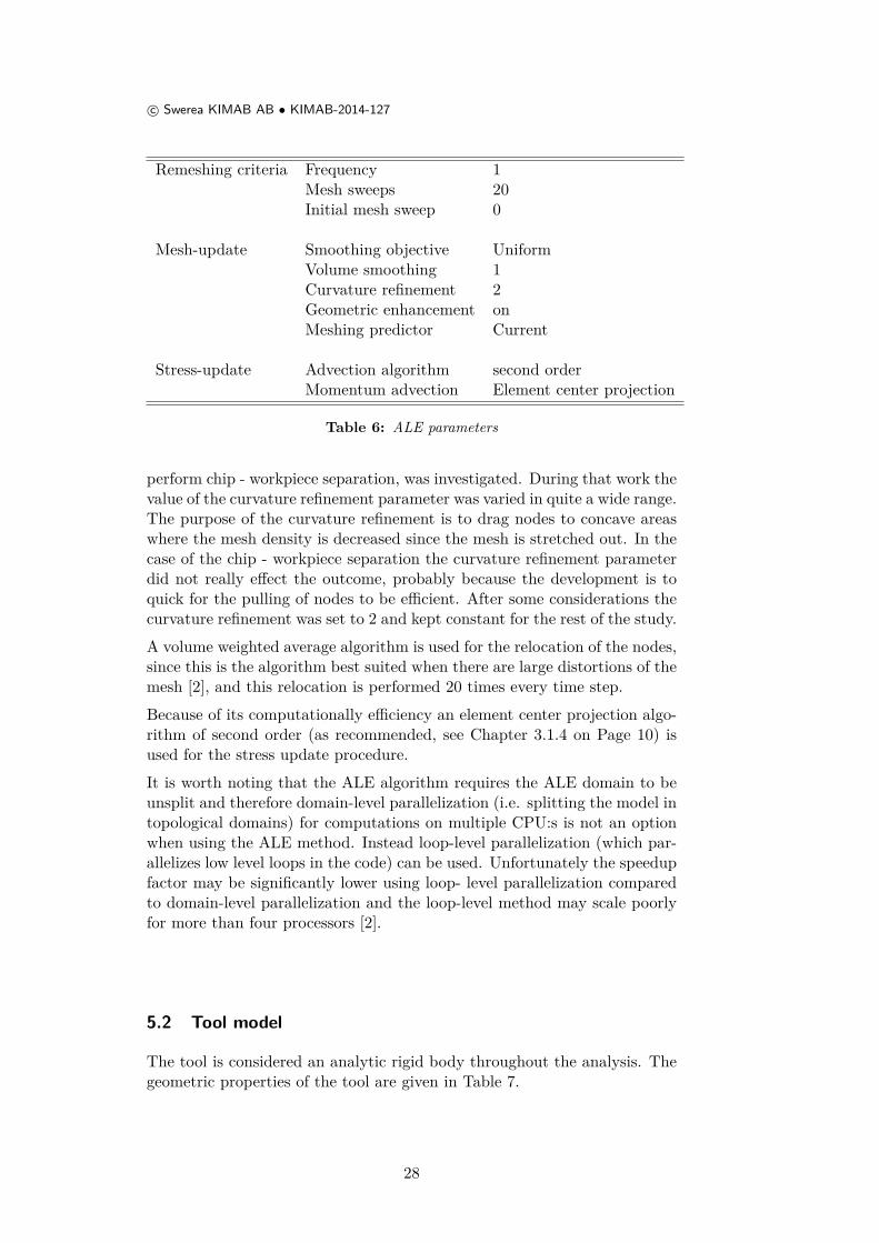
Remeshing criteria Frequency 1Mesh sweeps 20Initial mesh sweep 0

Mesh-update Smoothing objective UniformVolume smoothing 1Curvature refinement 2Geometric enhancement onMeshing predictor Current

Stress-update Advection algorithm second orderMomentum advection Element center projection

Table 6: ALE parameters

perform chip - workpiece separation, was investigated. During that work thevalue of the curvature refinement parameter was varied in quite a wide range.The purpose of the curvature refinement is to drag nodes to concave areaswhere the mesh density is decreased since the mesh is stretched out. In thecase of the chip - workpiece separation the curvature refinement parameterdid not really effect the outcome, probably because the development is toquick for the pulling of nodes to be efficient. After some considerations thecurvature refinement was set to 2 and kept constant for the rest of the study.

A volume weighted average algorithm is used for the relocation of the nodes,since this is the algorithm best suited when there are large distortions of themesh [2], and this relocation is performed 20 times every time step.

Because of its computationally efficiency an element center projection algo-rithm of second order (as recommended, see Chapter 3.1.4 on Page 10) isused for the stress update procedure.

It is worth noting that the ALE algorithm requires the ALE domain to beunsplit and therefore domain-level parallelization (i.e. splitting the model intopological domains) for computations on multiple CPU:s is not an optionwhen using the ALE method. Instead loop-level parallelization (which par-allelizes low level loops in the code) can be used. Unfortunately the speedupfactor may be significantly lower using loop- level parallelization comparedto domain-level parallelization and the loop-level method may scale poorlyfor more than four processors [2].

5.2 Tool model

The tool is considered an analytic rigid body throughout the analysis. Thegeometric properties of the tool are given in Table 7.

28


Rake angle, α[◦] +6Relief angle, c[◦] +6Tool nose radius, [µm] 20Cutting velocity, [m/min] 100

160260

Uncut chip thickness, [mm] 0.2

Table 7: Cutting conditions

Figure 7: Tool and workpiece boundary conditions

5.3 System model

Metal cutting can be performed in several ways and under several differentconditions. FE simulation of a system also require specific conditions, suchas contact conditions, to be explicitly defined.

5.3.1 Cutting conditions

A constant cutting velocity of 160 m/min (if nothing else is stated, in somesimulations a cutting velocity of 100 or 260 m/min is used) is applied to thetool in the negative x direction, all other degrees of freedom are constrained.The workpiece is fully restrained at the bottom surface and a symmetrycondition, in the x direction is applied at the left and at the lower part ofthe right surfaces as can be seen in Figure 7.

It is of great importance to note that the simulations are all performedwithout taking the temperature dependencies into account. This choice ismade, although heat effects have a major impact on the result of simulationsof machine cutting, in order to reduce the computational time and it doesnot falsify the conclusions from the investigation since the investigation isat a very initial step and no detailed results are needed.

29


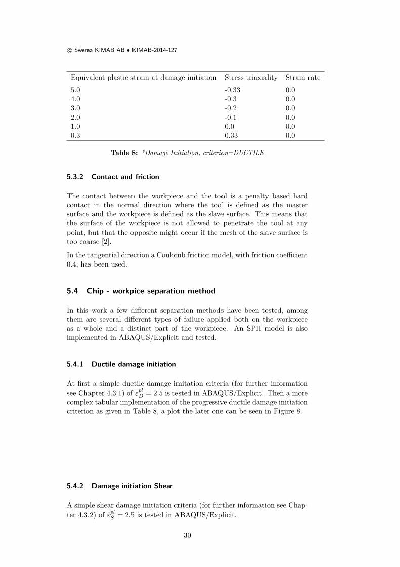
Equivalent plastic strain at damage initiation Stress triaxiality Strain rate5.0 -0.33 0.04.0 -0.3 0.03.0 -0.2 0.02.0 -0.1 0.01.0 0.0 0.00.3 0.33 0.0

Table 8: *Damage Initiation, criterion=DUCTILE

5.3.2 Contact and friction

The contact between the workpiece and the tool is a penalty based hardcontact in the normal direction where the tool is defined as the mastersurface and the workpiece is defined as the slave surface. This means thatthe surface of the workpiece is not allowed to penetrate the tool at anypoint, but that the opposite might occur if the mesh of the slave surface istoo coarse [2].

In the tangential direction a Coulomb friction model, with friction coefficient0.4, has been used.

5.4 Chip - workpice separation method

In this work a few different separation methods have been tested, amongthem are several different types of failure applied both on the workpieceas a whole and a distinct part of the workpiece. An SPH model is alsoimplemented in ABAQUS/Explicit and tested.

5.4.1 Ductile damage initiation

At first a simple ductile damage imitation criteria (for further informationsee Chapter 4.3.1) of εplD = 2.5 is tested in ABAQUS/Explicit. Then a morecomplex tabular implementation of the progressive ductile damage initiationcriterion as given in Table 8, a plot the later one can be seen in Figure 8.

5.4.2 Damage initiation Shear

A simple shear damage initiation criteria (for further information see Chap-ter 4.3.2) of εplS = 2.5 is tested in ABAQUS/Explicit.

30


−0.2 0 0.20

1

2

3

4

5

Triaxiality, η

Equivalent

plastic

strain

atda

mag

einitiation,εplD

Figure 8: Equivalent plastic strain at damage initiation, as a function oftriaxiality, for the ductile damage initiation according to Table 8.

D1 1.5D2 3.44D3 −2.12D4 0.002D5 0.1

Table 9: Johnson-Cook progresive damage parameters. From Agmell et al.[10]

5.4.3 Damage initiation Shear and Ductile

A combination of the progressive shear and ductile damage initiation crite-rion as used by Prasad [27] has also been tried. This criterion is on the formεplD = 1.5; εplS = 1.5, where these two separate damage initiation criteria areevaluated individually and then captured in a overall damage variable [2].

5.4.4 Johnson-Cook progressive Damage

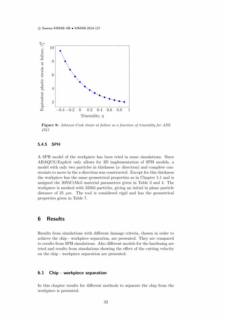
A Johnson-Cook dynamic failure model is tried for the AISI 4041 material.The Johnson-Cook damage parameters, as achieved from Agmell et al. [10],are given in Table 9. A plot of Johnson-Cook strain at failure as a functionof triaxiality is seen in Figure 9.

31


−0.4 −0.2 0 0.2 0.4 0.6 0.8 1

2

4

6

8

10

Triaxiality, η

Equivalent

plastic

strain

atfailu

re,ε

plf

Figure 9: Johnson-Cook strain at failure as a function of triaxiality for AISI4041

5.4.5 SPH

A SPH model of the workpiece has been tried in some simulations. SinceABAQUS/Explicit only allows for 3D implementation of SPH models, amodel with only two particles in thickness (z- direction) and complete con-straints to move in the z-direction was constructed. Except for this thicknessthe workpiece has the same geometrical properties as in Chapter 5.1 and isassigned the 20NiCrMo5 material parameters given in Table 3 and 4. Theworkpiece is meshed with 32563 particles, giving an initial in plane particledistance of 25 µm. The tool is considered rigid and has the geometricalproperties given in Table 7.

6 Results

Results from simulations with different damage criteria, chosen in order toachieve the chip - workpiece separation, are presented. They are comparedto results from SPH simulations. Also different models for the hardening aretried and results from simulations showing the effect of the cutting velocityon the chip - workpiece separation are presented.

6.1 Chip - workpiece separation

In this chapter results for different methods to separate the chip from theworkpiece is presented.

32


6.1.1 Ductile damage initiation tabular

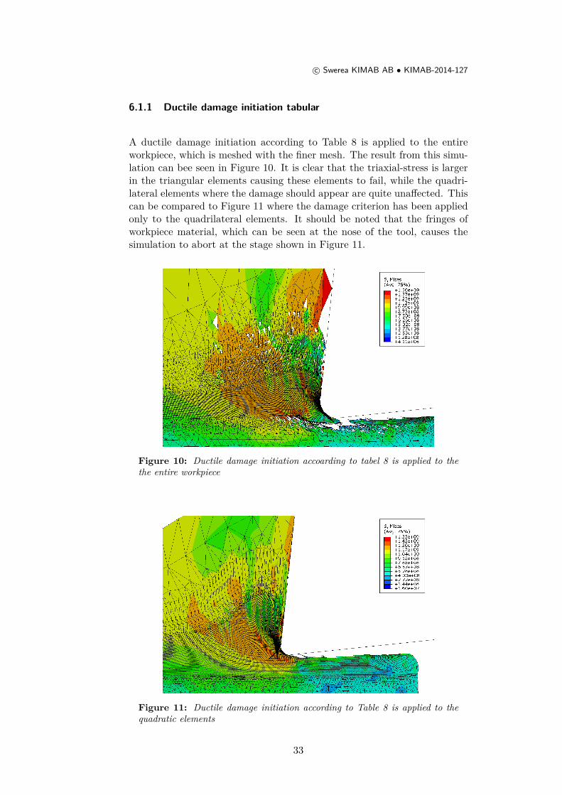
A ductile damage initiation according to Table 8 is applied to the entireworkpiece, which is meshed with the finer mesh. The result from this simu-lation can bee seen in Figure 10. It is clear that the triaxial-stress is largerin the triangular elements causing these elements to fail, while the quadri-lateral elements where the damage should appear are quite unaffected. Thiscan be compared to Figure 11 where the damage criterion has been appliedonly to the quadrilateral elements. It should be noted that the fringes ofworkpiece material, which can be seen at the nose of the tool, causes thesimulation to abort at the stage shown in Figure 11.

Figure 10: Ductile damage initiation accoarding to tabel 8 is applied to thethe entire workpiece

Figure 11: Ductile damage initiation according to Table 8 is applied to thequadratic elements

33


6.1.2 Damage initiation Shear

When applying a shear damage initiation criteria with εplS = 2, 5 in theentire workpiece a fringe is formed, by the crack that opens up along theshear band and, folded over the workpiece material. It should be notedthat a simulation with ductile damage initiation where εplD = 2, 5 would giveexactly the same result since the damage initiation in this case only dependson equivalent plastic strain.

Figure 12: Shear damage initiation of εplS = 2, 5 is applied in the entire

workpiece

6.1.3 Damage initiation Shear and Ductile

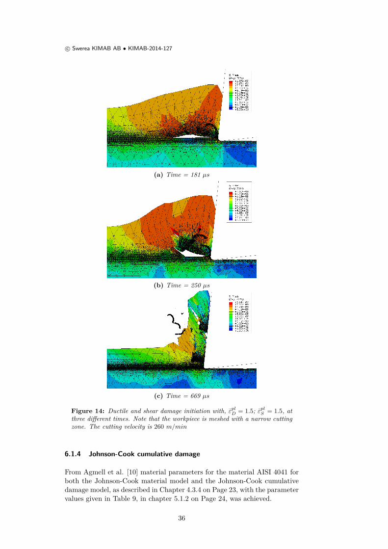
Using the combination of ductile and shear damage with, εplD = 1.5; εplS = 1.5,given by Prasad [27], the simulations runs without major element distortionerrors for a cutting velocity of 260 m/min. A simulation with these con-ditions can be seen in Figure 13. When running the simulation with aworkpiece mesh with only a narrow cutting zone the result is shown in Fig-ure 14. It can be seen that a large crack opens up in front of the tool tip ascan be seen in Figure 14a, then the crack tip moves up into the chip material(probably by shear effects) see Figure 14b and finally the chip is munchedtogether as seen in Figure 14c.

34


Figure 13: Ductile and shear damage initiation with, εplD = 1.5; εpl

S = 1.5,when the workpiece is meshed with a wide cutting zone. Simulation ran at acutting velocity of 260 m/min

35


(a) Time = 181 µs

(b) Time = 250 µs

(c) Time = 669 µs

Figure 14: Ductile and shear damage initiation with, εplD = 1.5; εpl

S = 1.5, atthree different times. Note that the workpiece is meshed with a narrow cuttingzone. The cutting velocity is 260 m/min

6.1.4 Johnson-Cook cumulative damage

From Agmell et al. [10] material parameters for the material AISI 4041 forboth the Johnson-Cook material model and the Johnson-Cook cumulativedamage model, as described in Chapter 4.3.4 on Page 23, with the parametervalues given in Table 9, in chapter 5.1.2 on Page 24, was achieved.

36


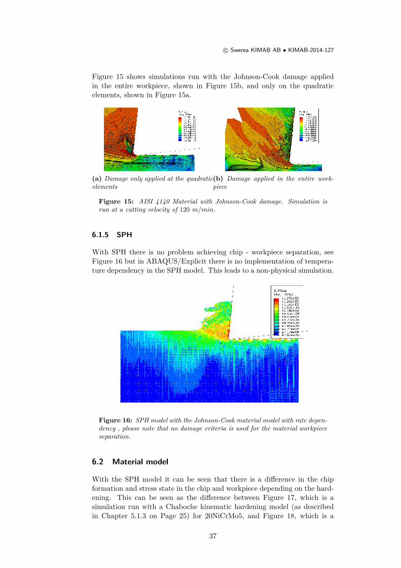
Figure 15 shows simulations run with the Johnson-Cook damage appliedin the entire workpiece, shown in Figure 15b, and only on the quadraticelements, shown in Figure 15a.

(a) Damage only applied at the quadraticelements

(b) Damage applied in the entire work-piece

Figure 15: AISI 4140 Material with Johnson-Cook damage. Simulation isrun at a cutting velocity of 120 m/min.

6.1.5 SPH

With SPH there is no problem achieving chip - workpiece separation, seeFigure 16 but in ABAQUS/Explicit there is no implementation of tempera-ture dependency in the SPH model. This leads to a non-physical simulation.

Figure 16: SPH model with the Johnson-Cook material model with rate depen-dency , please note that no damage criteria is used for the material workpieceseparation.

6.2 Material model

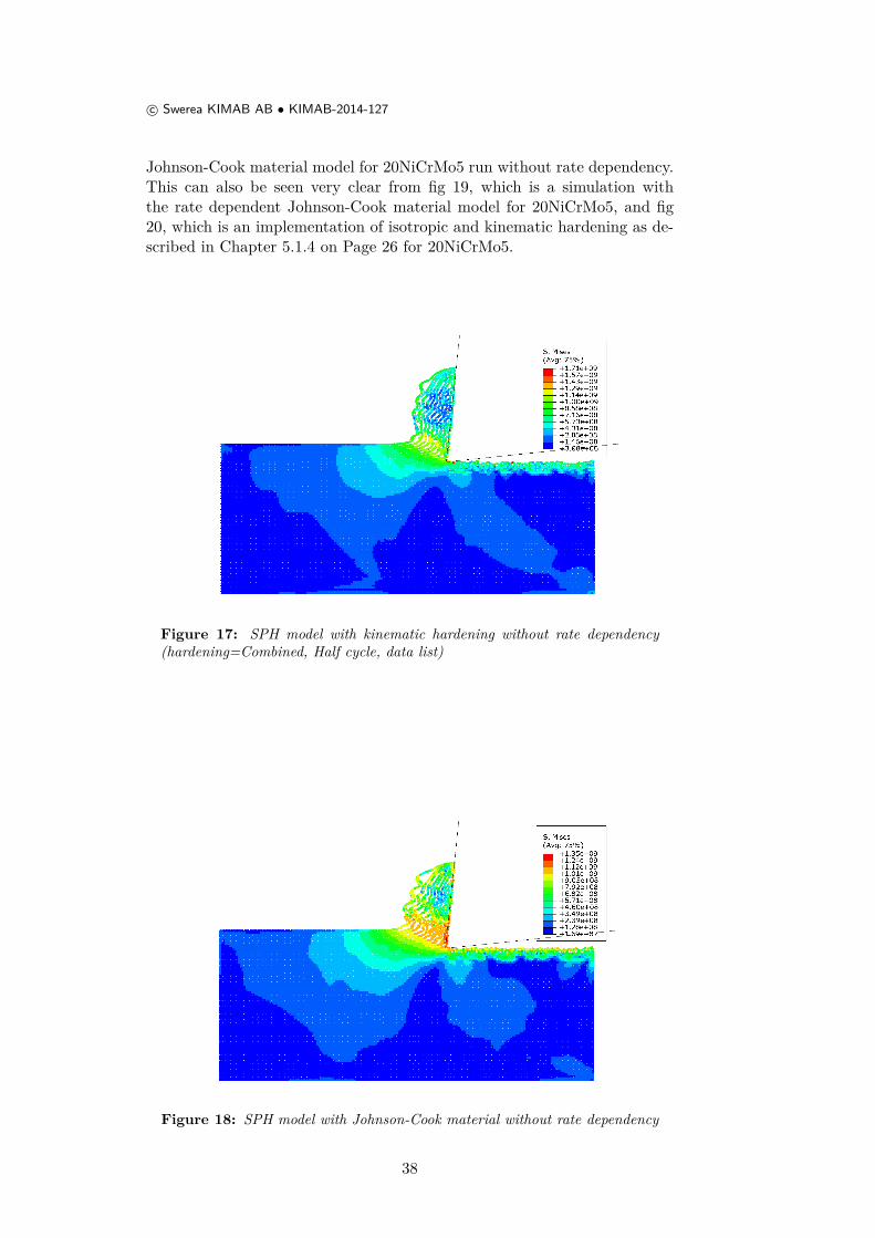
With the SPH model it can be seen that there is a difference in the chipformation and stress state in the chip and workpiece depending on the hard-ening. This can be seen as the difference between Figure 17, which is asimulation run with a Chaboche kinematic hardening model (as describedin Chapter 5.1.3 on Page 25) for 20NiCrMo5, and Figure 18, which is a

37


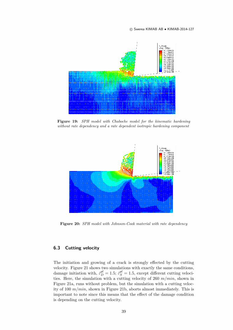
Johnson-Cook material model for 20NiCrMo5 run without rate dependency.This can also be seen very clear from fig 19, which is a simulation withthe rate dependent Johnson-Cook material model for 20NiCrMo5, and fig20, which is an implementation of isotropic and kinematic hardening as de-scribed in Chapter 5.1.4 on Page 26 for 20NiCrMo5.

Figure 17: SPH model with kinematic hardening without rate dependency(hardening=Combined, Half cycle, data list)

Figure 18: SPH model with Johnson-Cook material without rate dependency

38


Figure 19: SPH model with Chaboche model for the kinematic hardeningwithout rate dependency and a rate dependent isotropic hardening component

Figure 20: SPH model with Johnson-Cook material with rate dependency

6.3 Cutting velocity

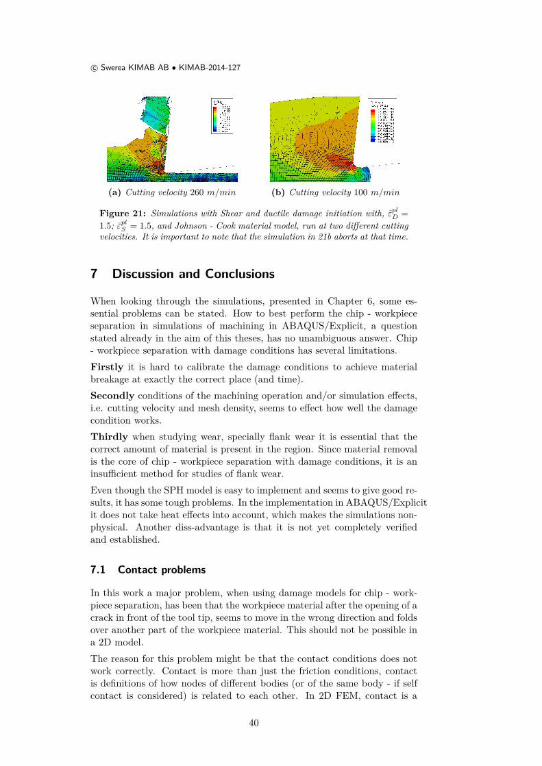
The initiation and growing of a crack is strongly effected by the cuttingvelocity. Figure 21 shows two simulations with exactly the same conditions,damage initiation with, εplD = 1.5; εplS = 1.5, except different cutting veloci-ties. Here, the simulation with a cutting velocity of 260 m/min, shown inFigure 21a, runs without problem, but the simulation with a cutting veloc-ity of 100 m/min, shown in Figure 21b, aborts almost immediately. This isimportant to note since this means that the effect of the damage conditionis depending on the cutting velocity.

39


(a) Cutting velocity 260 m/min (b) Cutting velocity 100 m/min

Figure 21: Simulations with Shear and ductile damage initiation with, εplD =

1.5; εplS = 1.5, and Johnson - Cook material model, run at two different cutting

velocities. It is important to note that the simulation in 21b aborts at that time.

7 Discussion and Conclusions

When looking through the simulations, presented in Chapter 6, some es-sential problems can be stated. How to best perform the chip - workpieceseparation in simulations of machining in ABAQUS/Explicit, a questionstated already in the aim of this theses, has no unambiguous answer. Chip- workpiece separation with damage conditions has several limitations.Firstly it is hard to calibrate the damage conditions to achieve materialbreakage at exactly the correct place (and time).Secondly conditions of the machining operation and/or simulation effects,i.e. cutting velocity and mesh density, seems to effect how well the damagecondition works.Thirdly when studying wear, specially flank wear it is essential that thecorrect amount of material is present in the region. Since material removalis the core of chip - workpiece separation with damage conditions, it is aninsufficient method for studies of flank wear.Even though the SPH model is easy to implement and seems to give good re-sults, it has some tough problems. In the implementation in ABAQUS/Explicitit does not take heat effects into account, which makes the simulations non-physical. Another diss-advantage is that it is not yet completely verifiedand established.

7.1 Contact problems

In this work a major problem, when using damage models for chip - work-piece separation, has been that the workpiece material after the opening of acrack in front of the tool tip, seems to move in the wrong direction and foldsover another part of the workpiece material. This should not be possible ina 2D model.The reason for this problem might be that the contact conditions does notwork correctly. Contact is more than just the friction conditions, contactis definitions of how nodes of different bodies (or of the same body - if selfcontact is considered) is related to each other. In 2D FEM, contact is a

40


relation between the nodes on a master surface and the nodes on a slavesurface. A surface is in this case defined as the line around a 2D area. Acontact "with self" is usually also defined in order to avoid that a body foldsover itself.

The problem here is that the nodes forming the workpiece surface changesas soon as the elements starts to fail. This does not seem to be a problemfor the tool - workpiece contact but it is a problem for the workpiece selfcontact.

In ABAQUS/Explicit there are two main sorts of contact: General contactand Contact pairs. Unfortunately the general contact option, which is easierto implement is only available to 3D models. When using general contactan internal surface can be defined which should solve the problem with thematerial folding over itself.

A solution could therefore be to make a one element thick model in 3D andrestrict it in the third direction so that it becomes a 2D model and apply ageneral contact condition having self contact with an internal surface.

As described in Chapter 5.3.2 two different types of friction has been tried.How they effect the result of a simulation of cutting is impossible to predictfrom the limited simulations performed in this study.

7.2 Mesh, elements and remeshing

In several of the simulations a problem is the formation of fringes that foldsover the workpiece material making it look like a double exposed picture.Some of the fringes like the one in Figure 12 is formed successively whenelements aligned with each other fails, and are therefore constituted of manyelements while other fringes like the ones in Figure 11 are constituted of onlya few very long elements.

A reason for these long elements, forming the fringes, could be that even withthe ALE remeshing algorithm used at maximum frequency, i.e. updating themesh at every time step, it can not really handle the problem with the meshgetting stretched out around the tool tip. The ALE algorithm only smoothsout the mesh, moving the nodes to improve element aspect ratio, while amesh refinement or a complete remeshing at the tool-tip would have beenneeded to preserve the undeformed shapes of the elements.

Another interesting thing one can observe is how the damage in the sec-ondary deformation zone effects the formation of the chip. When applyingdamage only in the quadrilateral elements the simulation terminates whenreaching the state shown in Figure 15a while applying damage in the entireworkpiece the simulation runs better and a chip is formed as shown in Fig-ure 15b. A possible reason for this is that it makes the sliding along therake face in the start up phase easier since elements of workpiece materialalong the rake face are deleted reducing the pressure between the tool andthe workpiece. It is also if interest to pay attention to the other side of thechip, i.e. not the part of the chip that is in contact with the rake face ofthe tool but the other side - that is freely exposed to the air, since it is here

41


breakage often occur in the real world. A physical phenomena of breakagein this part of the chip defines which type of chip is formed.

7.3 Conclusions

Many parameters effects the results of the simulations of machine cuttingfriction, temperature models, material models and so on. These parametersare linked together by complex internal relations, why it is complicated tostate how every single parameter act in the machining operation. Amongthe most important parameters for machining simulations are: the materialmodel (including correct temperature dependency and strain rate depen-dency over wide ranges), contact conditions and a correct description ofchip - workpiece separation.Even though the damage conditions can be trimmed to perform better thanpresented here, damage conditions are not directly related to the physicalprocesses they should model. Under some conditions cracks are formed inthe workpiece material but the main mechanism separating the chip fromthe workpiece is not usually related to fracture.The method of complete adaptive remeshing is today the most physicallycorrect and trustworthy choice for simulations of cutting. Although it iscomputationally expensive and not implemented in ABAQUS/Explicit.The SPH method, as implemented in ABAQUS/Explicit today, is not an op-tion since it has no temperature dependency. SPH simulations of machiningcould be performed in another simulation software, like LS-DYNA, wherethe SPH model has temperature dependency implemented. For simulationsin ABAQUS/Explicit, SPH might be a good choice in a few years time ifcoming releases of the software include temperature dependent SPH models.Further it seems like the type of hardening implemented in the materialmodel has an impact on the chip form, which is directly related to theloading on the tool and therefor effects the tool wear.

7.4 Future work

The SPH model needs to be further evaluated, preferably in another simu-lation software like LS-DYNA. An SPH model with a finer "mesh" should beimplemented and proper simulations with temperature dependency shouldbe run.A material model with a more correct implementation of the kinematichardening, containing strain rate effects and temperatures, could be triedin order to see whether there would be any improvements in the result inrelation to simulations with the ordinary Johnson-Cook material model.

8 Acknowledgements

I would like to express my gratitude to my supervisor at Swerea KIMAB, Dr.Niclas Stenberg, for guidance and support throughout simulations and writ-

42


ing. I would also like to thank my fellow thesis workers and other personnelat Swerea KIMAB for making my time here so joyful.

Last but not least, a big thanks to family and friends for their continuoussupport, love and encouragements.

This research has been performed in the framework of XPRES, Initiativefor excellence in production research.

9 References

References

[1] Dan Wedberg. Modelling of High Strain Rate Plasticity and Metal Cut-ting. PhD thesis, Luleå University of Technology, 2013.

[2] Inc. ABAQUS. Abaqus 6.13 Analysis User’s Guide. Technical report,2013.

[3] Xue Bin Liu, Xi Bin Wang, Chong Ning Li, and San Peng Deng. Fi-nite Element Simulation of the Orthogonal Cutting Based on Abaqus.Advanced Materials Research, 821-822:1410–1413, September 2013.

[4] P.J. Arrazola, A. Villar, D. Ugarte, and S. Marya. Serrated chip pre-diction in Finite Element modeling of the chip formation process. Ma-chining Science and Technology, (11):37–41, April 2014.

[5] Metal Cut diag by Emesee licensed under CC BY 3.0. http://en.wikipedia.org/wiki/Image:Metal_Cut_diag.jpg.

[6] Joanne Proudian. Simulating Residual Stress in Machining;From PostProcess Measurement to Pre-Process Predictions. M.Sc. thesis, RoyalInstitute of Technology. 2012.

[7] J Limido and C Espinosa. A new approach of high speed cutting mod-elling: SPH method. Journal de Physique IV, pages 1–6, 2006.

[8] Henrik Jäger. Quick-stop using the Buda test method in orthogonalturning turning. M.Sc. thesis, Uppsala University. 2014.

[9] M. Vaz, D. R. J. Owen, V. Kalhori, M. Lundblad, and L.-E. Lind-gren. Modelling and Simulation of Machining Processes. Archives ofComputational Methods in Engineering, 14(2):173–204, June 2007.

[10] Mathias Agmell, Aylin Ahadi, and JE Ståhl. The Link Between Plas-ticity Parameters and Process Parameters in Orthogonal Cutting. Pro-cedia CIRP, 00, 2013.

[11] Carl Johan Irander. Verifiering av simuleringsdata. FE-beräkningar ochmätmetoder för analys av skärande bearbetning. M.Sc. thesis, LuleåUniversity of Technology, 2004.

43

http://en.wikipedia.org/wiki/Image:Metal_Cut_diag.jpg

http://en.wikipedia.org/wiki/Image:Metal_Cut_diag.jpg


[12] L.-J. Xie, J. Schmidt, C. Schmidt, and F. Biesinger. 2D FEM estimateof tool wear in turning operation. Wear, 258(10):1479–1490, May 2005.

[13] Viktor P Astakhov. Tribology of Metal Cutting, volume 52. 2006.

[14] Bin Li. A review of tool wear estimation using theoretical analysis andnumerical simulation technologies. International Journal of RefractoryMetals and Hard Materials, 35:143–151, November 2012.

[15] David A. Stephenson and John S. Agapiou. Metal Cutting Theory andPractice. Taylor & Francis, 2:nd edition, 2005.

[16] Niels Saabye Ottosen and Matti Ristinmaa. The Mechanics of Consti-tutive Modeling. 2005.

[17] J Donea, Antonio Huerta, J Ponthot, and A Rodr. Chapter 14 Arbi-trary Lagrangian Eulerian Methods. In Erwin Stein, Rene de Borst,and Thomas J R Hughes, editors, Encyclopedia of Computational Me-chanics, chapter 14, pages 1–25. John Wiley & Sons, 2004.

[18] John David Jr. Anderson. Computational Fluid Dynamics: The Basicswith Applications. 1995.

[19] Morten F Villumsen and Torben G Fauerholdt. Simulation of MetalCutting using Smooth Particle Hydrodynamics. pages 17–36, 2008.

[20] J. Limido, C. Espinosa, M. Salaün, and J.L. Lacome. SPH methodapplied to high speed cutting modelling. International Journal of Me-chanical Sciences, 49(7):898–908, September 2007.

[21] J. Limido, C. Espinosa, M. Salaun, C. Mabru, R. Chieragatti, and J.L.Lacome. Metal cutting modelling SPH approach. International Journalof Machining and Machinability of Materials, 9(3/4):177, 2011.

[22] Martin Madaj and Miroslav Píška. On the SPH Orthogonal CuttingSimulation of A2024-T351 Alloy. Procedia CIRP, 8:152–157, January2013.

[23] M. Calamaz, J. Limido, M. Nouari, C. Espinosa, D. Coupard,M. Salaün, F. Girot, and R. Chieragatti. Toward a better understand-ing of tool wear effect through a comparison between experiments andSPH numerical modelling of machining hard materials. InternationalJournal of Refractory Metals and Hard Materials, 27(3):595–604, May2009.

[24] Eckart Uhlmann, Robert Gerstenberger, and Jörg Kuhnert. Cuttingsimulation with the meshfree Finite Pointset Method. 00, 2013.

[25] P. J. Arrazola, O. Barbero, and I. Urresti. Influence of material param-eters on serrated chip prediction in finite element modeling of chip for-mation Process. International Journal of Material Forming, 3(S1):519–522, June 2010.

44


[26] M. Issa, C. Labergère, K. Saanouni, and A. Rassineux. Numericalprediction of thermomechanical field localization in orthogonal cutting.CIRP Journal of Manufacturing Science and Technology, 5(3):175–195,January 2012.

[27] Chandra Shekhar Prasad. Finite element modeling to verify residualstress in orthogonal machining. M.Sc. thesis, Royal Institute of Tech-nology. 2009.

[28] P.J. Arrazola, T. Özel, D. Umbrello, M. Davies, and I.S. Jawahir. Re-cent advances in modelling of metal machining processes. CIRP Annals- Manufacturing Technology, 62(2):695–718, January 2013.

[29] E. Usui, T. Shirakashi, and T. Kitagawa. Analytical prediction of cut-ting tool wear. Wear, 100(1-3):129–151, December 1984.

[30] Yung-Chang Yen, Jörg Söhner, Blaine Lilly, and Taylan Altan. Es-timation of tool wear in orthogonal cutting using the finite elementanalysis. Journal of Materials Processing Technology, 146(1):82–91,February 2004.

[31] J. Lorentzon and N. Järvstråt. Modelling tool wear in cemented-carbidemachining alloy 718. International Journal of Machine Tools and Man-ufacture, 48(10):1072–1080, August 2008.

[32] Peter Gudmundson. Material Mechanics. 2006.

[33] Mohammad Sima and Tugrul Özel. Modified material constitutive mod-els for serrated chip formation simulations and experimental validationin machining of titanium alloy Ti-6Al-4V. International Journal ofMachine Tools and Manufacture, 50(11):943–960, November 2010.

[34] J Zouhar and M Piska. Modelling the orthogonal machining processusing cutting tools with different geometry. MM science Journal, pages49–52, 2008.

45

www.kth.se

Documents

A critical overview of machining simulations in ABAQUS866670/FULLTEXT01.pdf · DEGREE PROJECT, IN SOLID MECHANICS , SECOND LEVEL STOCKHOLM, SWEDEN 2014 A critical overview of machining