A Crisis of Missed Opportunities?Foreclosure Costs and Mortgage Modification

During the Great Recession∗

Stuart GabrielUniversity of California, Los Angeles

Matteo IacovielloFederal Reserve Board

Chandler LutzCopenhagen Business School

December 15, 2018

Abstract

We investigate the causal housing impacts of the 2000s crisis-period California Fore-closure Prevention Laws (CFPLs), policies that encouraged mortgage modifications bysubstantially increasing the lender pecuniary and time costs of foreclosure. The CFPLsprevented 248,000 California foreclosures (a reduction of 20.9%), increased California ag-gregate house prices by 6.2%, and created $350 billion of housing wealth. Findings alsoindicate that the CFPLs increased maintenance and repair spending for homes thatentered foreclosure, mitigating foreclosure externalities, while also boosting mortgagemodifications. The CFPLs had minimal adverse side effects in terms of the availabilityof mortgage credit for new borrowers. Altogether, the CFPLs were a highly effectiveforeclosure intervention that required no pecuniary subsidy from taxpayers.

JEL Classification: E52, E58, R20, R30 ;

Keywords: Foreclosure Crisis, Mortgage Modification, Great Recession

∗Gabriel: stuart.gabriel@anderson.ucla.edu. Iacoviello: matteo.iacoviello@frb.gov. Lutz: cl.eco@cbs.dk.Gabriel acknowledges funding from the UCLA Gilbert Program in Real Estate, Finance, and Urban Eco-nomics. Lutz acknowledges funding from the UCLA Ziman Center for Real Estate’s Howard and IreneLevine Program in Housing and Social Responsibility. Data and code available at https://github.com/

ChandlerLutz/CFPLCode.

1 Introduction and Background

At the height of the housing boom in 2005, California accounted for one-quarter of US housing

wealth.1 But as 2006 boom turned into 2008 bust, house prices in the state fell 30 percent

and over 800,000 homes entered foreclosure.2 To aid distressed borrowers, limit foreclosures,

and combat the crisis, the State of California pursued an alternative policy strategy that

increased foreclosure pecuniary costs and imposed foreclosure moratoria to incent widespread

lender adoption of mortgage modification programs. The aim of these policies was to stem

the rising tide of foreclosures, especially in areas like California’s Inland Empire that were

acutely hit by the crisis. Yet despite the application of a unique policy to a highly salient

housing market, there has been little focus on and no prior evaluation of California’s crisis

period policy efforts. In this paper, we undertake such an evaluation and use California as a

laboratory to measure the effects of the California Foreclosure Prevention Laws (CFPLs).

California is a non-judicial foreclosure state. Prior to the CFPLs, the state required only

that a lender or servicer (henceforth, lenders) initiating a home foreclosure deliver a notice

of default (NOD; foreclosure start) to the borrower by mail. A 90-day waiting period then

commenced before the lender could issue a notice of sale (NOS) of the property. In the midst

of the housing crisis in July 2008, California passed the first of the CFPLs, Senate Bill 1137

(SB-1137).3 This bill, which immediately went into effect, prohibited lenders from issuing an

NOD until 30 days after informing the homeowner via telephone of foreclosure alternatives.

The homeowner then had the right within 14 days to schedule a second meeting with the

lender to discuss foreclosure alternatives. SB-1137 additionally mandated that agents who

obtained a vacant residential property through foreclosure must maintain the property or face

steep fines of up to $1000 per day. The following year in June 2009, California implemented

the California Foreclosure Prevention Act (CFPA). The CFPA imposed an additional 90

day moratorium after NOD on lender conveyance of an NOS to borrowers unless the lender

implemented a State-approved mortgage modification program. Together, the CFPLs (SB-

1137 and the CFPA) significantly increased the lender pecuniary and time costs of home

foreclosure. A full overview of the CFPLs is in appendix A.

1ACS Table-S1101 and Zillow.2Mortgage Bankers’ Association3SB-1137 text.

1

The CFPLs were unique in scope and implemented at a moment when many California

housing markets were spiraling downward. As such, these policies provide a rare opportunity

to assess the housing impacts of important crisis-period policy interventions that sought to

reduce foreclosures and encourage mortgage modification.

From the outset, the CFPLs were viewed with skepticism. In marked contrast to the

California approach, the US Government elected not to increase foreclosure costs or dura-

tions during the crisis period. Indeed, Larry Summers and Tim Geithner, leading federal

policymakers, argued that such increases would simply delay foreclosures until a later date.4

However, findings of recent academic studies suggest mechanisms whereby the CFPLs

could have bolstered housing California housing markets. The key economic channel is based

on the negative price impacts of foreclosure on the foreclosed home (Campbell et al., 2011)

and neighborhood externalities, where foreclosures adversely affect nearby housing markets

by increasing housing supply (Anenberg and Kung, 2014; Hartley, 2014) or through a “dis-

amenity” effect where distressed homeowners neglect home maintenance (Gerardi et al., 2015;

Lambie-Hanson, 2015; Cordell and Lambie-Hanson, 2016). More broadly, a spike in foreclo-

sures lowers prices for the foreclosed and surrounding homes, which adversely affects local

employment (Mian and Sufi, 2014), and finally the combination of employment and house

prices losses leads to further foreclosures (Foote et al., 2008; Mian et al., 2015). By increasing

lender foreclosure costs, the foregoing research thus suggests that the CFPLs may have slowed

the downward cycle, mitigated the foreclosure externality, and buttressed ailing housing mar-

kets, especially in areas hard-hit by the crisis. Further, if the CFPLs reduced the adverse

effects of the foreclosure externality at the height of the crisis, then the policy effects should

be long lasting. These conjectures, however, have not been empirically tested, especially in

response to a positive, policy-induced shock like the CFPLs.

Figure 1 presents motivating evidence regarding the impacts of the CFPLs via plots of

housing indicators for California and the other Sand States. The blue dashed vertical lines

indicate the implementations of SB-1137 and the CFPA. Data sources are in the figure notes.

All Sand States behaved similarly prior to the CFPLs (e.g. the parallel pre-trends difference-

in-differences assumption). Then with the passage of the CFPLs, California foreclosures and

4Summars (2014); Geithner (2010a).

2

mortgage default risk fell markedly and housing returns increased; these effects persisted

through the end of the sample in 2014. In appendix B, we apply the Synthetic Control

method to these indicators and show that following the implementation of the CFPLs that

the improvement in the California housing market was exceptional compared to all other

states.

Below we exploit more disaggregated data, within California and across state variation,

and several estimation schemes to account for local housing and macro dynamics, loan-level

characteristics, and California-specific macro trends in our identification of policy effects.

We also emphasize our results surrounding the first of the CFPLs, SB-1137, which was im-

plemented immediately upon passage in July 2008. This law change thus yields a unique

opportunity for identification due its sharp timing and as it took effect early in the crisis be-

fore the announcement and implementation of the Federal Government’s HAMP and HARP

programs. Yet we document of the effects of the CFPLs on California housing over the entire

evolution of the crisis.

Our findings suggest that the CFPLs were highly effective in stemming the crisis in Cal-

ifornia foreclosures. The CFPLs prevented 248,000 Real Estate Owned (REO; NOS) fore-

closures, a reduction of 20.9%, and increased California aggregate housing returns by 6.2%.

In doing so, they created $350 billion of housing wealth. These effects were concentrated

in areas most severely hit by the crisis. We further provide direct evidence that the CFPLs

positively impacted housing markets using loan-level micro data: First we document that SB-

1137 caused an increase in home maintenance and repair spending by lenders who took over

foreclosed properties from defaulting borrowers, in line with the incentives of SB-1137 (recall

that SB-1137 mandated that agents who took over foreclosed properties must maintain them

or face fines of up to $1000 per day). This increased maintenance and repair spending directly

mitigates the foreclosure “disamenity” effect, a key reason why foreclosures create negative

externalities.5 As SB-1137 increased the cost of REO foreclosure via increased maintenance

and repair spending and as longer REO foreclosure durations (e.g. the time from the lender

takes over a foreclosed property to the time the property is disposed) are likely associated with

higher maintenance costs, one may expect lenders to respond by reducing REO foreclosure

5See (Gerardi et al., 2015; Lambie-Hanson, 2015; Cordell and Lambie-Hanson, 2016).

3

duration. This is a key policy goal of a foreclosure mediation strategy (Geithner, 2010b) and

what we find in our analysis of the policy, congruent with the CFPLs increasing foreclosure

costs. In other direct evidence of the CFPLs impact, we also show that the CFPLs increased

mortgage modifications. Specifically, we find that before the implementation of the Federal

Government’s HAMP and HARP programs that the CFPLs increased the mortgage modifi-

cation rate by 20%. Overall, our results suggest that the CFPLs were a successful crisis-era

intervention that required no pecuniary subsidies from taxpayers.

2 Data

We first estimate the effects of the CFPLs on the incidence of REO foreclosures using monthly

Zillow REO foreclosures per 10,000 homes at the county level. We complement this data with

controls and other variables compiled at the county level including Zillow house price returns;

Land Unavailability as a predictor for house price growth (Lutz and Sand, 2017); Bartik (1991)

labor demand shocks compiled from both the Census County Business Patterns (CBP) and

the BLS Quarterly Census of Employment and Wages (QCEW); household income from the

IRS Statistics of Income (SOI); the portion of subprime loan originated from HMDA data

and HUD subprime originator list; and the non-occupied homeowner occupation rate as this

may be a predictor of house price growth (Gao et al., 2017). We discuss these data in context

below and list all data in appendix C.

We also assess the effects of the CFPLs using loan-level data from the Fannie Mae and

Freddie Mac (GSE) loan performance datasets. While we have access to datasets that cover

non-conforming loans (e.g. Corelogic or Blackbox), we use GSE loan performance data for

two key reasons: First, the GSE data are publicly available, making our analysis transparent

and re-producible. Second, and just as important, the GSEs apply similar standards across

regions and do not discriminate based on geography (see Hurst et al. (2016) for a rigorous

treatment), meaning that the set of GSE loans yields natural controls and treatment groups

as regards the support of loan-level characteristics. We discuss our identification strategy for

our loan-level analysis in depth below.

4

3 Estimation Methodology: CFPLs and County REO Foreclosures

We employ two separate estimation schemes to measure the effects of the CFPLs on fore-

closures at the county level: The Synthetic Control method (Abadie et al., 2010, 2015) and

a difference-in-difference-in-differences approach. Our other analyses (for example loan-level

estimates) build on our approach described here; we discuss the differences in those sections.

Synthetic Control (Synth):

The Synth method generalizes the usual difference-in-differences, fixed effects estimator

by allowing unobserved confounding factors to vary over time. For a given treated unit,

Synth uses a data-driven algorithm to compute an optimal control from a weighted average

of potential candidates not exposed to the treatment. The weights are chosen to best approx-

imate the characteristics of the treated unit during pre-treatment period. For our foreclosure

analysis, we iteratively construct a Synthetic Control Unit for each California county, where

the characteristics used to build the Synthetic units are discussed below. The CFPL policy

effect is the difference (Gap estimate) between each California county and its Synthetic. For

inference, we conduct placebo experiments where we iteratively apply the treatment to each

control unit. We retain the Gap estimate from each placebo experiment and construct boot-

strapped confidence intervals for the null hypothesis of no policy effect (see also Acemoglu

et al. (2016)). For California counties where Gap estimates extend beyond these confidence

intervals, the CFPL effects are rare and large in magnitude.

Difference-In-Difference-In-Differences (DDD):

We also estimate the foreclosure impacts of the CFPLs through a DDD research design

that exploits a predictive framework that measures ex ante expected variation in REO fore-

closures within both California and across other states. Generally, the DDD approach allows

us to control for California-specific macro trends while comparing high foreclosure areas in

California to similar regions in other states (Imbens and Wooldridge, 2007; Wooldridge, 2011).

Our DDD specification for foreclosures is as follows:

5

Forc/10K Homesit =T∑

y=1y 6=2008M06

(θy1{y = t} × HighForci × CAi) (1)

+T∑

y=1y 6=2008M06

(1{y = t} × (β1yHighForci + β2yCAi + X′iλλλy))

+T∑

y=1

1{y = t}X′itγγγy

+ δt + δi + εit

The dependent variable is Zillow REO foreclosures per 10K homes. CA and HighForc

are indicators for California and high foreclosure counties, respectively. We define HighForc

below. The excluded dummy for indicator and static variables is 2008M06, the month prior

to the first CFPL announcement. The coefficients of interest are the interactions of monthly

indicators with CA and HighForc, θy.

We employ a full set of time interactions to (i) examine the parallel pre-trends assumption;

(ii) assess how quickly after implementation the CFPLs reduced REO foreclosures; and (iii)

determine if there is any reversal in the CFPL policy effects towards the end of the sample.

Intuitively for each month y, θy is the difference-in-difference-in-differences in foreclosures

where compare we ex ante “high foreclosure” counties to “low foreclosure” counties within

California (first difference); then subtract off the difference between high and low foreclosure

counties in other states (second difference); and finally evaluate this quantity relative to

2008M06 (third difference). The DDD estimates control for two potentially confounding

trends: (i) changes in foreclosures of HighForc counties across states that are unrelated to the

policy; and (ii) changes in California macro-level trends where identification of policy effects

through θy assumes that the CFPLs have an outsized impact in HighForc counties.

The cumulative CFPL DDD policy estimate over the whole CFPL period is Θ =∑

y≥2008M07 θy,

the total mean change in foreclosures for HighForc California counties. δt and δi are time and

county fixed effects, and all regressions are weighted by the number of households in 2000.

Controls (listed below) are fully interacted with the time indicators as their relationship with

foreclosures may have changed during the crisis.

We also examine the robustness of the foregoing DDD approach by mimicking equation 1

6

with the Synth estimates and regressing the Synth Gaps on HighForc interacted with month

indicators using only the California data in the final regression. This approach follows from

the observation that Synth Gap estimates are generalized difference-in-differences estimates

of California county-level foreclosures net of foreclosures in matched counties. The within

California regression then provides the third difference. As the final regression uses a smaller

California-only dataset, we retain county and time fixed effects but only interact the controls

with a CFPL indicator.

To measure the county-level pre-CFPL expected exposure to foreclosures (HighForc),

we forecast the increase (first-difference) in foreclosures (∆foreclosures) in each county for

2008Q3, the first CFPL treatment quarter, using only data up to 2008Q2 (pre-treatment

data). A random forest (RF) model is used to build the forecasts as RF models often pro-

vide more accurate predictions than traditional techniques (Mullainathan and Spiess, 2017;

Athey, 2018). We first train the RF model using data available up to 2008Q1 to predict

∆foreclosures for 2008Q2. We then predict ∆foreclosures for 2008Q3, the first CFPL treat-

ment quarter, using data up to 2008Q2. Predictors used in our RF model include the levels

and squared values of the first and second lags of ∆foreclosures; the first and second lag of

quarterly house price returns; the levels and squared 2007 unemployment rate; the interaction

of the unemployment rate (or its square) and the house price returns as the combination of

these quantities constitutes the double trigger theory of mortgage default (Foote et al., 2008);

the percentage of subprime originations in 2005 (Mian and Sufi, 2009); Land Unavailability

(Saiz, 2010; Lutz and Sand, 2017); an indicator for judicial foreclosure states (Mian et al.,

2015); the 2005 non-owner occupied mortgage origination rate as a proxy of housing market

speculation (Gao et al., 2017); and the maximum unemployment benefits for each county’s

state in 2007 (Hsu et al., 2018). Predictors also include 2007 income per household, a Sand

State indicator, and pre-CFPL Bartik (1991) Labor Demand Shocks. We also interact the

Bartik shocks with housing returns. Variable importance for each predictor in the RF model

is plotted in appendix D.

To gauge predictive accuracy, we evaluate our RF predictions relative to traditional OLS

models using the mean-squared error (MSE) for non-California counties in 2008Q3. The MSE

for the RF model is 36.5% lower relative to a benchmark panel AR(2), indicating that the RF

7

predictions are substantially more accurate. The MSE of the RF model is also 60.1% lower

than a full OLS model that includes all aforementioned predictors.

We classify counties as either high or low foreclosure (HighForc) based on the RF predic-

tions using a cross-validation approach. Specifically, we search from the US median predicted

change in foreclosures for 2008Q3 (1.64 per 10K homes) to the 90th percentile (13.07 per 10K

homes) and choose the cutoff for high foreclosure counties that minimizes the pre-treatment

difference between the treatment and control groups in equation 1 (the cutoff that minimizes∑y<2008M07 θ

2y). The cutoff chosen by the cross-validation procedure is 7.54 REO foreclosures

per 10K homes, corresponding to the 82nd percentile, meaning that HighForc counties have

a predicted increase in foreclosures of at least 7.54 per 10K homes for 2008Q3.

Note also that the RF model predicts marked foreclosure increases for the mean low

foreclosure California county at 5.28 REO foreclosures per 10K homes for 2008Q3 (nearly

five times the national median). Thus, there is room for foreclosures to fall in non-HighForc

California counties and allow the DDD estimates to account for California macro-level trends

that may lower foreclosures across the state.

The controls for the DDD model in equation 1 include the annual unemployment rate

and Bartik shocks; 2008M01-2008M06 house price growth; Land Unavailability; the 2005

non-owner occupied mortgage origination rate; the 2005 subprime origination rate; and 2007

income per household.

4 The Impact of the CFPLs on County-Level Foreclosures

The estimates of the CFPL impacts on REO foreclosures using the Synth and DDD ap-

proaches are visualized in figure 2. The county-level attributes used to build the Synth

matches for each California county use only pre-treatment data and include the following:

RF predictions for ∆foreclosures in 2008Q3, REO foreclosures, and variables used as controls

in equation 1.

Panel 1A plots the cumulative Gap in REO foreclosures at various percentiles for California

counties, where the percentiles are calculated within each month using only the California

county-level Synth Gap estimates. The two blue-dashed vertical lines are the implementations

of the SB-1137 and the CFPA, and the gray band is the 95% confidence interval bootstrapped

from all placebo experiments associated with the null of no CFPL policy effect. Gap estimates

8

that jut outside this confidence band are rare and large in magnitude.

During the pre-treatment period, the cumulative Gap is near zero across California per-

centiles, in line with the parallel pre-trends assumption. Then with passage of SB-1137 in

2008M07, REO foreclosures drop immediately for California counties at the 50th, 25th, and

10th percentiles. Counties at these percentiles are also bunched together towards the bottom

end of the distribution below the 95% confidence interval; the distribution is thus right-skewed

and a mass of California counties experienced a large and statistically significant CFPL drop

in REO foreclosures. The decline in foreclosures for these counties continued through 2014,

consistent with long lasting policy effects. Contrary to concerns expressed by federal policy-

makers, there is no evidence of reversal in aggregate county-level foreclosure trends. California

counties at the 75th or 90th percentiles experienced comparatively little foreclosure mitiga-

tion. This latter finding is not surprising given the pre-CFPL heterogeneity across California

housing markets.

The map in figure 2, panel 2 documents the geographic heterogeneity in CFPL foreclosure

reduction. Specifically, panel 2 shows the Synth cumulative Gap in REO foreclosures from

2008M07-2011M12. Red areas represent a reduction in foreclosures relative to the Synth

counterfactuals, gray areas indicate no change, blue areas correspond to an increase, and

white areas have no data. Names are printed on the map for counties whose cumulative Gap

is in the bottom 5th percentile relative to the empirical CDF of all placebo effects.

Overall, panel 2 shows that the areas most severely affected by the housing crisis also

experienced the largest CFPL treatment effects, in line with the policy successfully targeting

the most hard-hit regions. For example, San Bernardino and Riverside, lower income and

supply elastic regions that constitute California’s Inland Empire, were the epitome of the

2000s subprime crisis. These areas subsequently experienced large and beneficial CFPL pol-

icy effects: REO foreclosures per 10K homes in San Bernardino and Riverside fell by 428.25

(24.2%) and 379.74 (21.0%). Relative to the Synth counterfactuals, foreclosure reductions

were also large in Los Angeles and central California, as well as in inland Northern Califor-

nia. Interestingly, we find no CPFL policy effects in California’s wealthiest counties, located

around the San Francisco Bay (Marin, San Mateo, Santa Clara, and San Francisco). Com-

bining all of the Synth estimates across all California counties, results imply that the CFPLs

9

prevented 248,000 REO foreclosures, a reduction of 20.9%.

Panel 1B of figure 2 plots the estimation output of θy from equation 1. The red line

shows θy from a model that only includes time and county fixed effects (and the CA and

HighForc indicators). The green line corresponds to the full model with controls. Shaded

bands correspond to ±2 standard error (SE) bands where robust SEs are clustered at the

state level.

There are several key takeaways from panel 1B. First, the path of θy for the baseline and full

models is similar, indicating that the estimates are robust to the inclusion of controls. Next,

during the pre-treatment period, the ±2 SE bands subsume the horizontal origin and thus

the parallel pre-trends assumption is satisfied. Third and congruent with the foregoing Synth

estimates, θy falls immediately after the implementation of SB-1137 in 2008M07. Note that

HAMP and HARP, the federal mortgage modification programs, were announced in 2009M03

and not implemented in earnest until 2010M03.6 Thus the CFPL policy effects in California

substantially precede the announcement and implementation of the federal programs. Further,

θy levels off at approximately −10 in January 2009 and remains at these levels until 2012,

suggesting that the roll out of the federal programs did not change the path of θy. Fourth,

there are no reversals in the CFPL policy effects as θy stays below the zero-axis through the

end of the sample period, consistent with a mitigation of the foreclosure externality at the

peak of the crisis having a long-lasting impact on REO foreclosure reduction. Finally, the total

CFPL DDD estimate is (Θ =∑y=2011M12

y=2008M07 θy) = −451.44 (Robust F-statistic: 20.60); meaning

that for the average California HighForc county, the CFPLs reduced REO foreclosures by 451

per 10K homes. This estimate is in line with our above Synth results.

Last, panel 1C of figure 2 mimics equation 1 and panel 1B, but uses the Synth output and

only within California data as discussed above to estimate θy. Hence, panel 1C documents the

robustness of our results to an alternative, two-step estimation scheme. Overall, the path of

the estimates in panel 1C closely matches panel 1B, but the magnitudes are slightly smaller.

Specifically, θy in panel 1C hovers around the horizontal axis prior to 2008M07 in line with

the parallel pre-trends assumption; falls immediately after the implementation of SB-1137;

remains below the zero-axis and thus documents a reduction of foreclosures due to the CFPLs

6Agarwal et al. (2015, 2017) and their NBER working papers.

10

until 2012; and then returns to zero at the end of the sample period, implying no reversal in

policy effects.

4.1 CFPL DDD REO Foreclosure Estimate Robustness and Falsification Tests

This sections further assesses the robustness of the regression results from equation 1 presented

in panel 1B of figure 2. In particular, we first examine the parallel pre-trends assumption by

including county linear and quadratic time trends. The model of interest now becomes

Forc/10K Homesit =T∑

y=1y 6=2008M06

(θy1{y = t} × HighForci × CAi) (2)

+T∑

y=1y 6=2008M06

(1{y = t} × (β1yHighForci + β2yCAi + X′iλλλy))

+T∑

y=1

1{y = t}X′itγγγy

+ δt + δi +N∑i=1

ηi(δi × t) +N∑i=1

ζi(δi × t2) + εit

where ηi and ζi are the coefficients on linear and quadratic county time trends for each

of the i = 1, . . . , N counties. This model thus relaxes the pre-treatment common trends

assumption. Equation 2 includes both linear and quadratic trends as foreclosures may have

evolved non-linearly during the crisis. Note that the interpretation of coefficient of interest,

θy, is somewhat different from equation 1. Here θy measures the deviation from common

trends and thus the CFPL DDD effects will only be precisely estimated if the CFPLs induced

a sharp reduction in foreclosures in high foreclosure California counties (relative to control

regions) following the implementation of the CFPLs. In other words, these statistical tests

will reveal if CFPLs created an immediate drop in REO foreclosures.

In total, the results are in panels A and B of figure 3. Panel A plots θy only when the

regression model includes linear county time trends, while panel B employs both linear and

quadratic county time trends. The path of θy in panel A is nearly identical to our previous

estimates, providing further evidence that the parallel pre-trends assumption is satisfied and

that the CFPLs created a large drop in REO foreclosures immediately following their intro-

duction. In panel B where we include the both linear and quadratic time trends the estimates

for remain statistically significant, again implying that the parallel pre-trends assumption is

11

satisfied and that the CFPLs created a sharp drop in REO foreclosures for high foreclosure

California counties. Note in panel B that the standard error bands are slightly wider as the

inclusion of both linear and quadratic time trends reduces the degrees of freedom in the data.

The foregoing results show that CFPLs created a large and immediate drop in REO fore-

closures following their implementation. These results are robust to various housing and

macro controls, California macro trends, and region specific time trends. Further, the falsi-

fication tests executed within our Synthetic Control approach using non-California counties

(e.g. distribution of these falsification tests is shown by the gray band in panel 1A of figure

2) show that the change in REO foreclosures following the CFPLs was unique to California

relative to counties in all other states. Altogether, this evidence adds credence to the internal

validity of our estimates and a causal interpretation of our results. While below we provide

further evidence of the direct impact of the CFPLs at the loan-level, here we implement

additional, important falsification and robustness tests using aggregated, county-level data.

Indeed, the only remaining concern and threat to internal validity, from an aggregated data

perspective, is that a separate positive shock had an outsized impact on high foreclosure Cal-

ifornia counties right as the CFPLs were implemented in July 2008 and this positive shock

reduced foreclosures. We can explore the potential sources of these shocks by leaning on eco-

nomic theory: From the double trigger theory of mortgage default (Foote et al., 2008), that

says that households only default when they face negative equity and an adverse economic

shock, we infer that only an outsized economic shock or house price shock can generate the

effects like those documented above. We assess these shocks as potential confounders in turn.

First, we consider positive employment shocks. In our above estimates, we control Bartik

labor demand shocks. As these labor demand shocks are exogenous to the local housing

market (they are constructed through the interaction industry employment shares in 2000

and subsequent national growth), we include the Bartik shocks both before and after the

implementation of the CFPLs above as controls. In other words, our foregoing estimates

control for economic shocks to the local labor market during the pre-treatment and treatment

periods. Here we further assess the role of employment shocks through a falsification test over

the pre-treatment and treatment periods. In particular, we re-estimate our DDD regressions

but let the dependent variable be BLS QCEW Bartik shocks (we eliminate the CBP Bartik

12

shocks that were used above from our control set in this regression). If positive economic

shocks are the cause of the observed reduction in REO foreclosures, the DDD estimates

from this regression would be positive and large in magnitude. The results are in panel C

of figure 3. The results show that (1) there were no differences in economic shocks across

treatment and control groups during the pre-treatment period; (2) after the implementation

of SB-1137 in July 2008, the treatment group of high foreclosure California counties did

not experience positive, outsized economic shocks;7 and (3) there were no outsized economic

shocks following the implementation of the California Foreclosure Prevention Act in June

2009. These estimates therefore indicate that there were no positive employment shocks in

high foreclosure California counties relative to controls were not the cause of the decline

measured in our CFPL REO foreclosure DDD estimates.

Next, we examine the robustness of our results to changes in house prices directly following

the implementation of the CFPLs. Note that our above estimates are robust to the inclusion

Land Unavailability (a regional predictor of house price growth) and house price growth

during the first half of 2008 (prior to the implementation of the CFPLs) as controls. Yet as

stated above, if there was a large and positive house price shock at the same moment that the

CFPLs were implemented, the portion of homeowners facing negative equity and subsequently

foreclosures would decline. We address this concern by including an additional control, house

price growth in the second half of 2008 (2008Q3 & 2008Q4). While including house price

growth after the announcement and implementation of the CFPLs has the potential to be a

“bad control” (Angrist and Pischke, 2008), the rational for including this control is that a

reduction in foreclosures surfaces in house prices with a delay.8 Yet even if positive 2008Q3/4

house price growth was caused by the foreclosure reduction associated with the CFPLs, its

inclusion would simply bias our DDD CFPL foreclosure estimates towards zero. We present

the results in figure 3 where the DDD estimates associated with the model shown in red

only control for house price growth in the second half of 2008, while green line includes all

of the aforementioned controls. Equation 1 remains our estimation equation and in both

7The red line, the model with no controls, suggests that the control group experienced a small, negativeeconomic shock in January 2009. Only positive shocks are a threat to internal validity. Note also that oncecontrols are included (green line) that this that the magnitude of the Bartik DDD estimate is substantiallyreduced.

8Due to, for example, illiquidity in the housing market, especially during this period.

13

models we interact house price growth in 2008Q3/4 with a full set of time dummies (less the

excluded dummy) as in the second line of equation 1. The path of the CFPL REO foreclosure

DDD estimates are in panel D of figure 3. These results match our previous findings and

thus imply that house price changes at the moment of and immediately following the CFPL

implementation are not a potential confound for our estimates of the impact of the CFPLs on

foreclosures. Last, we note that the double theory of mortgage default specifies the interaction

of negative house price growth and adverse economic shocks as the catalyst for foreclosure

instantiation. Thus, we multiply 2008Q3/4 house price growth and Bartik shocks and use

this interaction as a control. The results are in panel E of figure 3. The path of the DDD

estimates matches our previous findings, meaning that the interaction of house price growth

and labor demand shocks are not a confounder for our results.

5 CFPL DDD REO Foreclosure Loan-Level Estimates

One potential concern with our above analysis is that loan-level characteristics may differ

across regions and thus contaminate our above results. While this is unlikely given the sharp

reduction in foreclosures immediately following the introduction of the CFPLs, we address

this concern here using GSE loan-level data. The key advantages of the GSE data are that

(1) they are publicly available; and (2) the GSEs do not discriminate across regions, yielding

loans that constitute natural control and treatment groups within a DDD analysis. Our

outcome of interest is the probability that a mortgage enters REO foreclosure and we aim to

estimate the DDD coefficients via a linear probability model that emulates equation 1. As

shown below, our results after accounting for loan-level characteristics match above findings

that employ county-level, aggregated data.

We proceed with estimation by employing a common two-step re-weighting technique

(Borjas, 1987; Card, 2001; Altonji and Card, 1991)9. This approach allows us to recover the

underlying micro, loan-level DDD estimates after controlling for loan-level characteristics,

while accounting for the fact that REO foreclosure and loan disposition are absorbing states

(e.g. once a loan enters REO foreclosure or is re-financed it is removed from the dataset) and

thus that the number of loans available in each region during each time period may in itself

depend on the treatment.

9For more recent references, see Angrist and Pischke (2008); Beaudry et al. (2012); Lutz et al. (2017).

14

In the first step we estimate the following loan-level regression, where noting that the

lowest level of geographic aggregation in the GSE loan performance data are three digit zip

codes:

Prob(REO Forc)it =T∑

y=1

N∑i=1

(ρiy × 1{y = t} × zip3i) +T∑

y=1

N∑i=1

(1{y = t}X′iτττ iy) + eit (3)

The dependent variable is an indicator that takes a value of 1 for REO foreclosure and

zero otherwise. ρiy are the year-month coefficients on zip3× 1{y = t} dummy variables and

τiy are the coefficients on Loan × 1{y = t} loan-level characteristics. Hence, we allow the

impact of loan-level characteristics on the probability of REO foreclosure to vary flexibly with

time as the predictive power of these characteristics may have changed with the evolution

of the crisis. Broadly, equation 3 allows us to quality-adjust and thus purge our estimates

from any bias associated with differences in loan-level characteristics. We estimate equation

3 using only loans originated during the pre-treatment period as loans originated subsequent

to the CPFLs may have been affected by program treatment. Similarly, the vector of loan

characteristics used as controls are only measured at loan origination as time-varying variables

(such as current unpaid principal balance) may also be impacted by program treatment. Xi

includes a wide array of loan characteristics which are listed in the notes to figure 4 that

shows our final estimation output.

From the regression in equation 3 we retain the zip3-month coefficient estimates on the

zip3 dummies, ρiy. In the second step of the estimation process, we employ the following

model that yields the DDD estimates of the impact of the CFPLs on the probability of REO

foreclosure using loan-level data (slightly changing the subscripts on ρ to match equation 1):

ρit =T∑

y=1y 6=2008M06

(θy1{y = t} × HighForci × CAi) (4)

+T∑

y=1y 6=2008M06

(1{y = t} × (β1yHighForci + β2yCAi + X′iλλλy))

+ X′itγγγy + δt + δi + εit

θy is the DDD coefficient of interest and represents the impact of the CFPLs on loans in

high foreclosure California zip3 regions after controlling for the change in the probability of

15

foreclosure in low foreclosure California zip3 regions and the difference in the change in the

foreclosure rate between high and low foreclosure zip3 regions in other states. We determine

high foreclosure California zip3 regions based on the Random Forest predictions and process

documented above. Aggregate controls include Land Unavailability as well as CBP and BLS

QCEW Bartik labor demand shocks.

The results are in figure 4. The second-step regression in equation 4 is weighted by the

number of households in 2000 and robust standard errors are clustered at the state level. The

vertical axis in the plot is in basis points as the probability of REO foreclosure during a given

month for a loan is quite small.

The path of θy in panel A figure 4 (both with and without extra macro and housing

controls) is similar to our previous DDD estimates in figures 2 and 3, implying that our

estimates of the impact of the CPFLs on REO foreclosures are robust the inclusion of loan-

level characteristics as controls.

First, during the pre-treatment period, θy is a precisely estimated zero, indicating that

the parallel pre-trends assumption is satisfied. Indeed, the F-statistic associated the DDD

estimate with the cumulative probability that a loan enters REO foreclosure during the pre-

treatment period (∑

y<2008M07 θy) is 0.61 (p-value = 0.44).

Then with the announcement and implementation of the SB-1137 in July 2008, the first

of the CFPLs, the probability of REO foreclosure for high foreclosure California zip3 regions

falls immediately and sharply. The quick drop in the probability of REO foreclosure, even

after controlling for loan-level characteristics and macro controls, buttresses the assertion

that the reduction in high foreclosure California counties was due to the CFPLs: Before the

announcement of HAMP in 2009M03, the probability that a mortgage in a high foreclosure

California region succumbed to REO foreclosure (∑2009M02

y=2008M07 θy) fell by 19.29 basis points.

Compared to the counterfactual of non-California high foreclosure regions where the pre-

HAMP treatment period probability of REO foreclosure was 51.24 basis points (2008M07-

2009M02); the DDD estimate represents a 38 percent decline in the REO foreclosure rate

due to the CFPLs. The cluster-robust F-statistic associated with this DDD estimate during

the pre-HAMP treatment period (∑2009M02

y=2008M07 θy) is 20.96 (p-value < 0.001), meaning that

the reduction in the REO foreclosures following the implementation of SB-1137 and the

16

introduction of the CFPLs was both large and statistically significant.

From there, θy stays below zero through 2011 as the CFPLs continued to reduce foreclo-

sures in high foreclosure California regions over evolution of the crisis. θy then reverts back

to zero (and becomes statistically insignificant) in late 2011 into 2012. Importantly, θy does

not ascend above zero through the end of the sample period, in line with our above results

that show that the CFPLs simply did not delay REO foreclosures until a later date.

Panel B of figure 4 controls for zip3 time trends and therefore assesses the parallel pre-

trends assumption and if the CFPLs induced an immediate and sharp drop in the REO

foreclosure rate. The path of θy is nearly identical across panels A and B of figure 4. Hence,

the parallel pre-trends assumption appears to be satisfied as our results are robust to the

inclusion of local housing market time trends.

Another possibility is that homes in high foreclosure California regions were are being

disposed by a foreclosure alternative (Short Sale, Third Party Sale, Charge Off, or Note

Sale). While foreclosure alternatives may reduce the number of empty homes in these regions,

such resolutions would not have aided policymakers in their goal of keeping homeowners in

their homes. We repeat the above analysis, but let the dependent variable be equal to 1

for mortgages that enter into a foreclosure alternate and zero otherwise. The path of the

DDD coefficients is in appendix E. The results show that there was no change in incidence

of foreclosure alternates during the early part of the crisis. Then, beginning in mid-2009,

foreclosure alternates in high foreclosure California regions began to drop, meaning that the

probability that a mortgage entered into a foreclosure alternative fell.

6 Foreclosure Maintenance and Repair Costs

In this section, we provide direct evidence that the CFPLs increased foreclosure costs by fo-

cusing on foreclosure maintenance and repair costs for homes in REO foreclosure. Recall that

a key provision of SB-1137 was that agents who took over a home via REO foreclosure must

maintain the home or face fines of to $1000 per property per day. This implies that policymak-

ers believed that (1) homes obtained via REO foreclosure were not being properly maintained

and (2) that the foreclosure externality “disamenity effect” was exacerbating the foreclosure

crisis. Indeed, as noted in the introduction, previous research shows that “disamenity effects”

are a key contributor to foreclosure externalities and thus limiting disamenity effects, by in-

17

centivizing home maintenance for example, will reduce foreclosures within a housing market.

Further, increasing foreclosure costs changes the net-present-value calculation of foreclosure

relative to modification.

From the GSE loan performance data, we retain all loans that enter REO foreclosure. For

each REO foreclosure, the GSEs report the amount spent on maintenance and repairs for each

home before disposition. The pre-treatment and CFPL treatment groups are based on the

REO foreclosure date. For the pre-treatment group, we consider all homes that entered REO

foreclosure before the announcement of the CFPLs and whose disposition date was also before

the announcement of the CFPLs. REO foreclosures in the CFPL treatment period include

only loans whose REO foreclosure date is after the announcement of SB-1137, but before the

announcement of HAMP in 2009M03. Thus, these data include no loans that entered into

REO foreclosure after the announcement of HAMP. Note that we drop all REO foreclosures

where the REO foreclosure date is before SB-1137 but the disposition date is after SB-1137,

as the GSEs only report total foreclosure costs and not foreclosure spending by month. With

this data in hand, we estimate a DD regression where the dependent variable is foreclosure

maintenance and repair costs:

Forc Maintenance and Repair Costsit = α + γi + δt + θ(CAi × CFPLt) + X′iλλλ+ εit (5)

where the left-hand-side variable measures foreclosure maintenance and repair costs in

dollars, γi is zip3 fixed effects, δt represents REO foreclosure date fixed effects, and the

coefficient of interest, the DD estimate θ, captures the increase in foreclosure costs due to

the SB-1137. Note that given our definition of the treatment and control groups (based on

REO foreclosure date and disposition date), that the duration of time spent in foreclosure

(and thus foreclosure costs) may vary with the REO foreclosure date. We account for this by

including linear and quadratic effect effects in the months spent in REO foreclosure as well

as REO foreclosure date fixed effects.

The results for non-judicial states are in table 1, those for all states are in appendix

F. Column (1) of table 1 shows the results without any fixed effects or controls. Average

foreclosure maintenance and repair costs for non-California properties during the pre-CFPL

period was $3016.11. The coefficient on CA is near zero at $57.89 dollars with a standard error

18

of $270.29, implying that there were no average level differences in pre-treatment foreclosure

spending across the treatment and controls groups and thus that the parallel pre-trends

assumption is satisfied. This result is congruent with our expectations as the GSEs do not

discriminate based on geography (Hurst et al., 2016). The coefficient on CFPL is $478.73

and statistically significant, meaning that the during the CFPL period for non-California

foreclosures that the GSEs spent nearly 16% more on average for maintenance and repairs

than during the CFPL period. The coefficient on the CA × CFPL interaction, the DD

estimate, is $573.78 and statistically significant. This coefficient estimate suggests that on

average that the increase in spending on foreclosure maintenance and repair doubled for

California properties relative to non-California properties during the CFPL period.

Column (2) of table 1 adds linear and quadratic effects in the time spent in REO fore-

closure. As expected, longer REO foreclosure durations correspond to higher maintenance

spending. Yet the quadratic term is negative, suggesting that monthly spending falls as du-

rations lengthen. This may due to the fixed costs associated with foreclosure maintenance or

unwillingness of agents to spend on foreclosure maintenance at longer durations. Notice again

that the coefficient on CA is insignificant, indicating that there are no level differences in pre-

treatment foreclosure maintenance spending across treatment and control groups. Also, once

we control for foreclosure durations, the coefficient on CFPL falls by half, but the coefficient

on the CA × CFPL interaction only changes slightly. Comparing average foreclosure mainte-

nance spending after accounting for foreclosure durations suggests that increase in foreclosure

maintenance spending during the CFPL period was more than twice as high for California

foreclosures relative to those in other states. Columns (3), (4), and (5) cumulatively add REO

foreclosure date fixed effects, zip3 fixed effects, and loan-level controls respectively. The in-

cluded loan-level controls are listed in the notes to table 1. The coefficient on the CA × CFPL

interaction attenuates somewhat, but still remains large in magnitude and highly significant.

Finally, columns (6) and (7) add linear and quadratic REO foreclosure date zip3 time trends.

These tests allow us to assess the pre-trends assumption and the DD coefficients will only be

precisely estimated if there is a sharp increase in foreclosure costs following the introduction

of SB-1137. In columns (6) and (7) the DD coefficient is again large and magnitude and

highly significant and thus implying that even after allowing for uncommon trends that there

19

was a large and statistically significant increase in foreclosure maintenance and repair costs

for California properties.

6.1 REO Foreclosure Durations

The above section documents that the CFPLs induced agents who took over homes via REO

foreclosure to increase maintenance and repair spending. Further, if the extra maintenance

spending comprised marginal costs associated with length of time in foreclosure (e.g. lawn

maintenance for example), we would expect rational agents to circumvent these costs by dis-

posing of homes obtained through REO foreclosure quicker. In other words, REO foreclosure

durations may shorten. Indeed, shortening REO foreclosure durations is a key policy objec-

tive as empty homes contribute to the foreclosure “disamenity effect” and exacerbated the

housing crisis (Geithner, 2010b).

Using a DD analysis, we assess the impact of the CFPLs REO foreclosure durations in

table 2. Foreclosures are split into the pre-treatment and treatment groups as in section 6.10

Columns (1) - (3) show the results for non-judicial states only, while columns (4) - (6) display

the regression output where the dataset comprises all states. Loan-level controls match those

from table 1 and robust standard error errors are clustered at the state level. Column (1)

controls only for REO foreclosure date fixed effects (as the foreclosure durations vary with

REO foreclosure date given how we split foreclosures into treatment and control groups). The

middle panel shows that during the CFPL period, that average REO foreclosure duration for

non-California properties in non-judicial states was 7.97 months. The coefficient on CA is near

zero at 0.057 (less than one-tenth of a month) with a standard error of 0.301, indicating that

there was no levels differences in average REO foreclosure durations during the pre-treatment

period and thus that the parallel pre-trends assumption is satisfied. The coefficient on the

CA × CFPL interaction is −0.662, indicating that foreclosure durations fell by over half a

month for California properties. Yet as this coefficient is imprecisely estimated, it is not

statistically significant at conventional levels. Columns (2) and (3) add zip3 fixed effects

and loan controls, respectively. The coefficient on the CA × CFPL interaction with a full

set of controls remains stable at −0.589, but its standard error falls markedly and therefore

10Note that the regressions in table 2 use more observations than those in table 1 because foreclosure andmaintenance spending is missing for some REO foreclosures.

20

implying that the zip3 fixed effects and loan-level controls are uncorrelated with the CFPL

treatment implementation in California but have predictive power for foreclosure durations.

The DD coefficient in column (3) is statistically significant at conventional levels, indicating

that the CFPLs shortened REO foreclosure durations.

Columns (4) - (6) show the results for all states. Overall the DD estimates are similar,

but the standard errors are smaller as the sample size increases. This yields larger t-statistics.

The coefficient on the CA × CFPL interaction in column (6), that includes all controls, is

−0.475 with a standard error of 0.215. Congruent with our above results, this statistically

significant DD estimate means that the CFPLs shortened foreclosure durations by just under

a half of a month during the CPFL period.

7 Mortgage Modifications

While the overarching aim of the CFPLs was to reduce foreclosures, the policy also sought

to increase modifications. This sections uses GSE loan-level data to assess the change in

the modification rate due to the CFPLs. We employ the same two-step estimation procedure

described above in section 5, but in this case the outcome variable of interest is the probability

of loan modification. Step 1 of the two step procedure is identical to that described in section

5, but we use an indicator for mortgage modification as the left-hand-side variable. In the

second step, we estimate the following DD regression:

ρit =T∑

y=1y 6=2008M06

(1{y = t} × (θyCAi + X′iλλλy)) + X′itγγγy + δt + δi + εit (6)

where ρit are the coefficient estimates on zip3 × time dummy variables from the first step

of the procedure that control for loan-level characteristics. The coefficient of interest is θy

that measures the difference-in-differences in the probability of loan modification in California

relative to other states. δi and δt are zip3 and year-month fixed effects and the static and

time varying controls include zip3 land unavailability as well as CBP and BLS QCEW Bartik

shocks, respectively. The regression is weighted by the number of households in 2000 and

robust standard errors are clustered at the state level.

The DD regression here is of interest as θy measures, after controlling for loan-level char-

acteristics, the change in the probability of mortgage modification induced by the CFPLs in

21

California.

We plot the estimation output of θy from the above equation in panel A of figure 5. The

vertical axis is in basis points. The path of θy shows that there is no pre-treatment difference

in the modification rate prior to the CFPLs, meaning that the parallel pre-trends assumption

is satisfied (to the left of the first blue-dashed vertical line). Then with the passage of SB-1137

in July 2008, we see a statistically significant increase in the modification rate. Recall that

HAMP and HARP were not announced until March 2009 (and not implemented until March

2010 (Agarwal et al., 2015, 2017)). Thus prior to the announcement of the Federal programs,

the CFPLs caused an increase in the modification rate of 4.05 basis points (∑2008M03

y=2008M07 θy).

While this may seem small, note that the modification rate in general is small. For the

counterfactual non-California regions during the pre-HAMP treatment period, the probability

of mortgage modification was just 10.59 basis points. Together, these estimates imply that

the SB-1137 increased the modification rate by a 38 percent.

Then following the implementation of the California Foreclosure Prevention Act in June

2009, the modification rate increased markedly. Note that the rollout of HAMP and HARP

did not begin until March 2010 (Agarwal et al., 2015, 2017) and thus the increase in mod-

ifications due to the CFPA proceeded the implementations of the Federal programs. From

the announcement of the CFPLs in July 2008 to February 2010, just prior the implementa-

tion of HAMP and HARP (∑2008M03

y=2008M07 θy) was 22.56 basis points. The associated F-statistic

is 13.74 (p-value < 0.001). Thus, the increase in modifications induced by the CFPLs was

large in magnitude and statistically significant. Using data through end the end of 2012, the

estimated increase in the modification rate due the CFPLs is 130.89 basis. A back of the

envelope application of this estimate applied to all of California mortgages during the CFPL

period suggests that CFPLs led to an additional 70,000 mortgage modifications, without re-

quiring any pecuniary subsidies from taxpayers. In contrast, nationwide HAMP subsidized

both lenders and borrowers but led to just 1 million modifications (Agarwal et al., 2017).

Using the total number of housing units with a mortgage from the ACS Survey, the above

estimates imply that the CFPLs induced 68 percent of the modification increases relative

to HAMP without any pecuniary subsidies.11 HAMP also did not include any provisions to

11Using the estimate that HAMP created 1 million modifications from Agarwal et al. (2017) and datafrom table B25081 from the 1-year 2007 ACS survey, suggests that the modification rate for HAMP was

22

increase foreclosure costs like the CFPLs.

Panel B controls for zip3 time-trends. The estimates match our above findings, implying

that the parallel pre-trends assumption is satisfied and that CFPLs led to an deviation in the

modification rate relative to local trends.

8 CFPL Foreclosure Reduction and House Price Growth

Extant research suggests that foreclosures reduce prices for foreclosed homes and neighboring

homes through a supply response or a “disamenity” effect. Indeed, an extensive literature

aims to estimate the effects of foreclosures on house prices, but none do so in response to a

positive policy induced shock (foreclosure mitigation) during a crisis.12 Previous studies also

largely focus on neighborhood effects, while our analysis benefits from a large-scale policy

experiment in the nation’s largest housing market. We thus contribute to the literature by

measuring the causal impact of CFPLs on house prices and estimating aggregate price effects

in response to foreclosure reduction. These findings also provide insight as to the spatial

impact of mortgage defaults and foreclosure mitigation policies.

We estimate the house price impacts of CFPL foreclosure alleviation through a three-

step approach that mimics a DDD design. First, we retain our Synth REO foreclosure Gap

estimates (figure 2, panel 2), the difference-in-differences in foreclosures for each California

county relative to their Synth counterfactuals.

Our dependent variable is CFPL house price growth at the zip code level. Clearly, Cali-

fornia house prices may change for reasons unrelated to the CFPLs (such as broader housing

recovery). Thus, we next obtain the abnormal house price growth for each California zip

code – analogous to an abnormal equity return – through Synth Gap estimates.13 For each

California zip code, we apply the Synth method and retain the Gap estimate for house price

growth during the CFPL period.

We plot the median CFPL house price growth Gap estimate within each California county

in figure 6, panel 1. The notes to figure 6 list the variables used to build the zip code Synthetic

1,000,000/51,962,570 = 0.019. In comparison the modification rate computed above for the CFPLs was 0.013.Thus 0.013/0.019 = 68.4. The number of California housing units with a mortgage from that same ACSsurvey is 5,381,874. Thus 5,381,874 * 0.013089 = 70,443.35 modified California mortgages.

12Campbell et al. (2011); Anenberg and Kung (2014); Gerardi et al. (2015); Fisher et al. (2015); Mianet al. (2015).

13Abnormal Return = Actual Return− Expected Return

23

counterfactuals. The county names printed on the map are from figure 2. Generally, in

counties where the CFPLs lowered foreclosures, like San Bernardino, house prices increased.

We test this visual anecdote more formally as the third step in our estimation scheme in

figure 6, panel 2A. Here we regress the Gap in CFPL house price growth on the Gap in CFPL

REO foreclosures within California (weighted by the number of households in 2000). County

foreclosure Gap estimates are mapped to zip codes using the Missouri Data Bridge. The slope

estimates in panel 2A are DDD CFPL estimates that measure the increase in house prices

due to a decline in foreclosures. Using OLS, the slope is −0.029 (robust SE clustered at the

three-digit zip code level: 0.009), while the median slope from a quantile regression that is

robust to outliers is −0.033 (robust SE: 0.003). Appendix G shows the point estimates from

panel 2A, and re-estimates these regressions controlling for the 2009-2011 Bartik shock as well

as 2007 household income and levels house prices, proxies of zip code income and housing

wealth. The estimates are similar.

Using the median slope estimate (−0.033) and the median CFPL Synth Gap decline in

REO foreclosures per 10K homes (−303.48), CFPL REO foreclosure reduction increased hous-

ing returns for the median zip code by 10.02%. Applying the distribution of REO foreclosure

quantile regression estimates across California implies that the CFPLs increased California

aggregate house price returns by 6.2% ($350 billion).

Finally, figure 6, panel 2B assesses shows mean abnormal house price growth for CFPL

REO foreclosure reduction quintiles. The plot shows that the impact of CFPL REO fore-

closure reduction on house prices is concentrated in cases where there was large, but not

extremely large, REO foreclosure reduction. For counties in the second quintile in terms of

CFPL REO foreclosure reduction, abnormal house prices increased 13 percent. In areas with

the minimal foreclosure reduction (e.g. quintiles 4 and 5), there was little abnormal house

price changes.

9 Did the CFPLs Create Adverse Side Effects for New Borrowers?

The CFPLs increased the lender foreclosure costs and thus ex post, may have reduced the

value of the lender foreclosure option. As noted by Alston (1984), if the value of the foreclosure

option declines, lenders may respond by either (1) increasing interest rates on new mortgages

to compensate for the depreciation of the foreclosure option; or (2) rationing credit, especially

24

in environments where raising interest rates is infeasible.14 For the CFPLs, (1) would translate

into fewer loans being originated in California post-policy, ceteris paribus. With regard to

(2), Alston notes that during the Depression, lenders were reluctant to increase interest rates

as this would have created “hostility and ill will” (p. 451). Similar concerns may have also

deterred lenders from increasing interest rates in California following housing crisis.

Conversely, in their report on the CFPA, California (2010) notes that the number of appli-

cations for an exemption from the CFPA foreclosure moratorium was lower than anticipated,

suggesting that the lender value of the foreclosure option was limited given the depths of the

crisis. Also if the CFPLs aided depressed California housing markets (as documented above),

then lenders may have viewed the CFPLs favorably as foreclosures can create dead weight

losses for lenders (Bolton and Rosenthal, 2002).

We employ the HMDA dataset to determine the impact of the CFPLs on mortgage credit

following the implementation of the policy. We only consider loans not sold to GSEs as GSEs

do not discriminate based on region (Hurst et al., 2016). The results are in table 3. First,

we use loan-level data to determine whether the probability of being denied a mortgage is

higher in California, in line with a credit rationing response for new borrowers following the

CFPLs. Specifically, we consider a linear probability model where the dependent variable is

an indicator that equals one for mortgage loan denial.15 The key independent variable is an

indicator for mortgages originated in California. Controls are listed in the notes to table 3

and the data range from 2009 to 2014. We first restrict the dataset to Arizona, California,

Florida, and Nevada (column (1)), as the housing dynamics of these states were similar during

the 2000s; for robustness we also consider a dataset with California, Colorado, New York, and

Texas (column (2)), states that were less affected by and rebounded quickly from the crisis.

Robust standard errors are clustered at the 3-digit zip code level. A positive coefficient on

California would suggest that Californians were more likely to be denied mortgage credit. If

anything, the results in columns (1) and (2) show opposite: The probability of denial in post-

CFPL California was slightly lower. Hence, Californians were no more likely than residents

in the other states to be denied mortgage credit in the wake of the CFPLs.

Columns (3) - (6) examine loan volume growth following the implementation of the CFPLs.

14Lenders ration credit as underwriting costs increase (Sharpe and Sherlund, 2016).15We do not know if denied mortgages would have eventually been sold.

25

We consider loan growth at the zip code level, both in terms of the number and dollar volume

of loans, for 2009 through 2014 relative to 2007 using only loans not sold to GSEs. The key

independent variable is an indicator for California and robust standard errors are clustered

at the commuting zone level. Here, if mortgage lenders were rationing credit to California zip

codes, relative to those in other states, the coefficient on California would be negative. Again,

we find the opposite effect. The estimates imply that loan volume growth was instead higher

in California zip codes. In total, the results in table 3 show that new California borrowers

were not adversely affected by the CFPLs.

10 Discussion

Our above Synth results show that the CFPLs prevented 248,000 REO foreclosures in Cal-

ifornia. Our estimated effects are large in magnitude relative to other federal government

programs. Outside of California, HAMP and HARP, the federal mortgage modification pro-

grams prevented approximately 230,000 and 80,000 REO foreclosures respectively (Agarwal

et al., 2015, 2017).16 Also note that HAMP and HARP are not a threat to identification as

the CFPL effects preceded the announcement and implementation of the federal programs

(figure 2). Similarly outside of California, Hsu et al. (2018) find that unemployment insurance

prevented 500,000 REO foreclosures. Hence relative to these other programs, the impact of

the CFPLs on foreclosures is large in magnitude. The CFPLs were also relatively costless

compared to these other programs as they did not provide pecuniary subsidies to lenders and

borrowers (HAMP/HARP) or to unemployed households (unemployment insurance).

A potential concern not previously addressed is unemployment insurance as a confounding

factor. Although our DDD analysis controls for California-level trends, we explicitly account

for unemployment insurance here by re-estimating our Synth foreclosure results using only

states within the same quintile as California in terms of crisis-era unemployment benefits

based on data from Hsu et al. (2018). Using this alternate control group, the CFPLs lowered

REO foreclosures by 426,000 (31.3%), making our above results conservative in nature.

Our above Synth analysis also employs judicial and non-judicial states in the control group,

whereas California is a non-judicial foreclosure state. Re-estimating our Synth results using

only non-judicial states in the control group suggests that the CFPLs reduced foreclosures by

16Numbers from Hsu et al. (2018) and the Mortgage Bankers’ Association.

26

20.4%, in line with our above estimates.

Other states also proposed legislation to impose foreclosure moratoria, but to our knowl-

edge none of these proposed bills matched the breadth of the CFPLs and most were not

enacted.17 One state-level intervention did occur in Massachusetts, who passed a foreclosure

right-to-cure law in 2008. Gerardi et al. (2013) find that the law did not improve borrower

foreclosure outcomes. Unlike the Massachusetts law, the CFPLs were larger in scope and

implemented when California housing markets faced extreme distress. Our results are robust

to the exclusion of Massachusetts as a control. Yet the inclusion of Massachusetts does not

pose a threat to identification as positive effects owed to the Massachusetts law would bias

our results towards zero.

10.1 External Validity

While the aim of this paper is to establish internal validity for estimates of the impact of

the CFPLs on California, external validity (e.g. other instances where similar policies were

implemented) is of interest as well. We discuss external validity in the context of other

research. One noteworthy instance of external validity arises from the Great Depression and

the study of farm foreclosure moratoria. This analysis was carried out by Rucker and Alston

(1987). Congruent with the our analysis of the CFPLs during the recent crisis, Rucker and

Alston find that the farm foreclosure moratoria reduced farm foreclosure during the Great

Depression. Further, Mian et al. (2015) study judicial and non-judicial states during crisis

and conclude that the increased costs associated with judicial foreclosure limited foreclosure

instantiation. Note that, however, there is debate regarding robustness of the impacts of

judicial foreclosure (Gerardi et al., 2013). While the CFPLs were similar in some aspects to

the aforementioned policies, they were unique in their scope and implementation: The CFPLs

directly incentivized foreclosure maintenance spending, while also encouraging modifications

through foreclosure moratoria. Overall, the efficacy of the CFPLs matches the extant research

on foreclosures, while Rucker and Alston document that moratoria, a portion of the CFPL

response, provided foreclosure relief during the Great Depression.

17See 2008-2009 proposed (but not enacted) legislation: Connecticut, Massachusetts (link1, link2, link3),Michigan (link1, link2, link3), Minnesota, South Carolina (link1, link2), Illinois, and Arkansas. Nevadaimplemented a foreclosure mediation program in 2009M07.

27

11 Conclusion

In this paper, we estimate the impacts of the California Foreclosure Prevention Laws. Our

results show that the CFPLs prevented 248,000 REO foreclosures and created $350 billion in

housing wealth. These results are large in magnitude, economically meaningful, and show how

the CFPLs, a foreclosure intervention that did not require any pecuniary subsidies, boosted

ailing housing markets. A back of the envelope application of our estimates to non-California,

high foreclosure counties indicates that the implementation of the CFPLs in these counties

would have prevented an additional 104,000 REO foreclosures and created $71 billion in

housing wealth.

28

References

A. Abadie, A. Diamond, and J. Hainmueller. Synthetic control methods for comparativecase studies: Estimating the effect of California’s tobacco control program. Journal of theAmerican Statistical Association, 105(490), 2010.

A. Abadie, A. Diamond, and J. Hainmueller. Comparative politics and the synthetic controlmethod. American Journal of Political Science, 59(2):495–510, 2015.

D. Acemoglu, S. Johnson, A. Kermani, J. Kwak, and T. Mitton. The value of connections inturbulent times: Evidence from the United States. Journal of Financial Economics, 121(2):368–391, 2016.

S. Agarwal, G. Amromin, S. Chomsisengphet, T. Piskorski, A. Seru, and V. Yao. Mort-gage refinancing, consumer spending, and competition: Evidence from the home affordablerefinancing program. Technical report, National Bureau of Economic Research, 2015.

S. Agarwal, G. Amromin, I. Ben-David, S. Chomsisengphet, T. Piskorski, and A. Seru. Pol-icy intervention in debt renegotiation: Evidence from the home affordable modificationprogram. Journal of Political Economy, 125(3):654–712, 2017.

L. J. Alston. Farm foreclosure moratorium legislation: A lesson from the past. The AmericanEconomic Review, 74(3):445–457, 1984.

J. G. Altonji and D. Card. The effects of immigration on the labor market outcomes of less-skilled natives. In Immigration, trade, and the labor market, pages 201–234. University ofChicago Press, 1991.

E. Anenberg and E. Kung. Estimates of the size and source of price declines due to nearbyforeclosures. American Economic Review, 104(8):2527–51, 2014.

J. D. Angrist and J.-S. Pischke. Mostly Harmless Econometrics: An Empiricist’s Companion.Princeton University Press, 2008.

S. Athey. The impact of machine learning on economics. Working Paper, 2018.

T. J. Bartik. Who Benefits from State and Local Economic Development Policies? Booksfrom Upjohn Press. W.E. Upjohn Institute for Employment Research, November 1991.

P. Beaudry, D. A. Green, and B. Sand. Does industrial composition matter for wages? a testof search and bargaining theory. Econometrica, 80(3):1063–1104, 2012.

P. Bolton and H. Rosenthal. Political intervention in debt contracts. Journal of PoliticalEconomy, 110(5):1103–1134, 2002.

G. J. Borjas. Immigrants, minorities, and labor market competition. ILR Review, 40(3):382–392, 1987.

California. California foreclosure prevention act report. Technical report, California Depart-ment of Corporations, 2010.

J. Y. Campbell, S. Giglio, and P. Pathak. Forced sales and house prices. American EconomicReview, 101(5):2108–31, 2011.

D. Card. Immigrant inflows, native outflows, and the local labor market impacts of higherimmigration. Journal of Labor Economics, 19(1):22–64, 2001.

29

M. Chauvet, S. Gabriel, and C. Lutz. Mortgage default risk: New evidence from internetsearch queries. Journal of Urban Economics, 96:91–111, 2016.

L. Cordell and L. Lambie-Hanson. A cost-benefit analysis of judicial foreclosure delay and apreliminary look at new mortgage servicing rules. Journal of Economics and Business, 84:30–49, 2016.

L. M. Fisher, L. Lambie-Hanson, and P. Willen. The role of proximity in foreclosure exter-nalities: Evidence from condominiums. American Economic Journal: Economic Policy, 7(1):119–40, 2015.

C. L. Foote, K. Gerardi, and P. S. Willen. Negative equity and foreclosure: Theory andevidence. Journal of Urban Economics, 64(2):234–245, 2008.

Z. Gao, M. Sockin, and W. Xiong. Economic consequences of housing speculation. Workingpaper, 2017.

T. Geithner. Geithner calls foreclosure moratorium ‘very damaging’, 2010a. Online; posted10-October-2010.

T. Geithner. Tim geithner interview with charlie rose, 2010b. Online; posted 10-October-2010.

K. Gerardi, L. Lambie-Hanson, and P. S. Willen. Do borrower rights improve borroweroutcomes? evidence from the foreclosure process. Journal of Urban Economics, 73(1):1–17,2013.

K. Gerardi, E. Rosenblatt, P. S. Willen, and V. Yao. Foreclosure externalities: New evidence.Journal of Urban Economics, 87:42–56, 2015.

D. Hartley. The effect of foreclosures on nearby housing prices: Supply or dis-amenity?Regional Science and Urban Economics, 49:108–117, 2014.

J. W. Hsu, D. A. Matsa, and B. T. Melzer. Unemployment insurance as a housing marketstabilizer. American Economic Review, 108(1):49–81, 2018.

E. Hurst, B. J. Keys, A. Seru, and J. Vavra. Regional redistribution through the us mortgagemarket. The American Economic Review, 106(10):2982–3028, 2016.

G. Imbens and J. Wooldridge. Difference-in-differences estimation, 2007.

R. Koenker and K. F. Hallock. Quantile regression. Journal of economic perspectives, 15(4):143–156, 2001.

L. Lambie-Hanson. When does delinquency result in neglect? mortgage distress and propertymaintenance. Journal of Urban Economics, 90:1–16, 2015.

C. Lutz and B. Sand. Highly disaggregated land unavailability. Working Paper, 2017.

C. Lutz, A. Rzeznik, and B. Sand. Local economic conditions and local equity preferences:Evidence from mutual funds during the us housing boom and bust. 2017.

A. Mian and A. Sufi. The consequences of mortgage credit expansion: Evidence from the usmortgage default crisis. The Quarterly Journal of Economics, 124(4):1449–1496, 2009.

A. Mian and A. Sufi. What explains the 2007–2009 drop in employment? Econometrica, 82(6):2197–2223, 2014.

30

A. Mian, A. Sufi, and F. Trebbi. Foreclosures, house prices, and the real economy. TheJournal of Finance, 70(6):2587–2634, 2015.

S. Mullainathan and J. Spiess. Machine learning: an applied econometric approach. Journalof Economic Perspectives, 31(2):87–106, 2017.

R. R. Rucker and L. J. Alston. Farm failures and government intervention: A case study ofthe 1930’s. The American Economic Review, 77(4):724–730, 1987.

A. Saiz. The geographic determinants of housing supply. Quarterly Journal of Economics,125(3), 2010.

S. A. Sharpe and S. M. Sherlund. Crowding out effects of refinancing on new purchasemortgages. Review of Industrial Organization, 48(2):209–239, 2016.

L. Summars. Lawrence Summers on ‘House of Debt’, 2014. Online; posted 6-June-2014.

J. Wooldridge. Difference-in-differences estimation. http://www.eief.it/files/2011/10/

slides_6_diffindiffs.pdf, 2011.

31

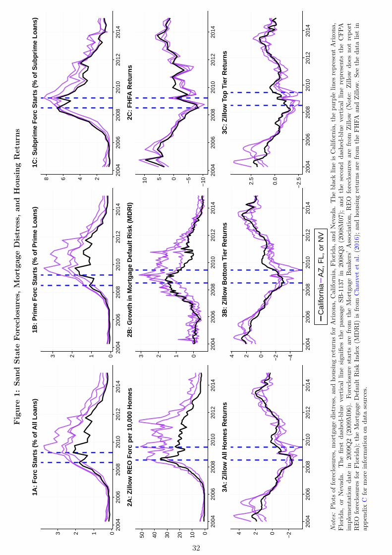
Fig

ure

1:

Sand

Sta

teFore

closu

res,

Mort

gage

Dis

tress

,and

Housi

ng

Retu

rns

0123

2004

2006

2008

2010

2012

2014

1A: F

orc

Sta

rts

(% o

f All

Loan

s)

0123

2004

2006

2008

2010

2012

2014

1B: P

rime

For

c S

tart

s (%

of P

rime

Loan

s)

2468

2004

2006

2008

2010

2012

2014

1C: S

ubpr

ime

For

c S

tart

s (%

of S

ubpr

ime

Loan

s)

01020304050

2004

2006

2008

2010

2012

2014

2A: Z

illow

RE

O F

orc

per

10,0

00 H

omes

0123

2004

2006

2008

2010

2012

2014

2B: G

row

th in

Mor

tgag

e D

efau

lt R

isk

(MD

RI)

−10−

50510

2004

2006

2008

2010

2012

2014

2C: F

HFA

Ret

urns

−2024

2004

2006

2008

2010

2012

2014

3A: Z

illow

All

Hom

es R

etur

ns

−4

−2024

2004

2006

2008

2010

2012

2014

3B: Z

illow

Bot

tom

Tie

r R

etur

ns

−2.

5

0.0

2.5

2004

2006

2008

2010

2012

2014

3C: Z

illow

Top

Tie

r R

etur

ns

Cal

iforn

iaA

Z, F

L, o

r N

V

Notes:

Plo

tsof

fore

clos

ure

s,m

ortg

age

dis

tres

s,an

dh

ousi

ng

retu

rns

for

Ari

zon

a,

Cali

forn

ia,

Flo

rida,

an

dN

evad

a.

Th

eb

lack

lin

eis

Cali

forn

ia,

the

pu

rple

lin

esre

pre

sent

Ari

zon

a,

Flo

rid

a,or

Nev

ada.

Th

efi

rst

das

hed

-blu

ever

tica

lli

ne

sign

ifies

the

pass

age

SB

-1137

in2008Q

3(2

008M

07);

an

dth

ese

con

dd

ash

ed-b

lue

ver

tica

lli

ne

rep

rese

nts

the

CF

PA

imp

lem

enta

tion

dat

ein

2009

Q2

(200

9M06

).F

orec

losu

rest

arts

are

from

the

Mort

gage

Ban

kers

’A

ssoci

ati

on

,R

EO

fore

closu

res

are

from

Zil

low

(Note

:Z

illo

wd

oes

not

rep

ort

RE

Ofo

recl

osu

res

for

Flo

rid

a);

the

Mor

tgag

eD

efau

ltR

isk

Ind

ex(M

DR

I)is

from

Ch

au

vet

etal.

(2016);

an

dh

ou

sin

gre

turn

sare

from

the

FH

FA

an

dZ

illo

w.

See

the

data

list

inap

pen

dix

Cfo

rm

ore

info

rmat

ion

ond

ata

sou

rces

.

32

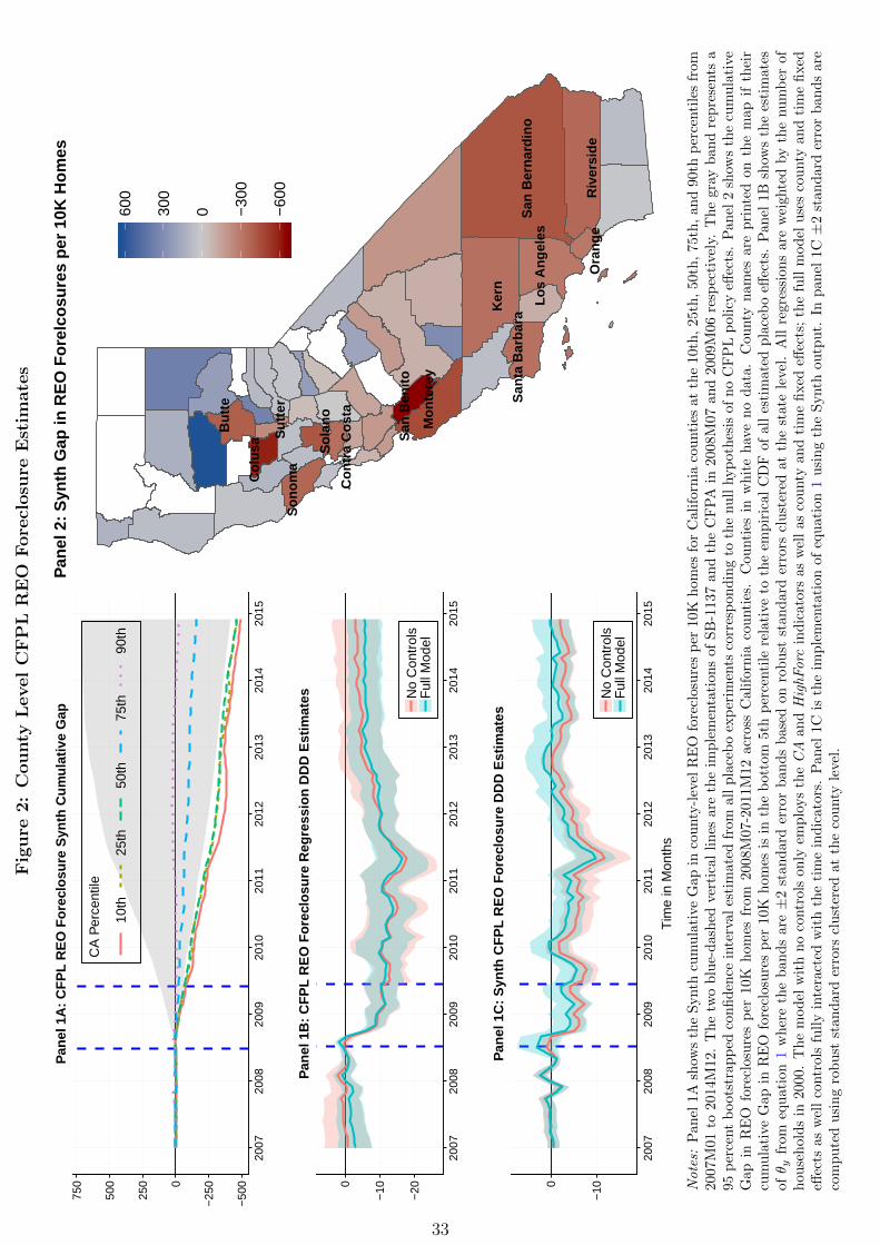
Fig

ure

2:

County

Level

CF

PL

RE

OFore

closu

reE

stim

ate

s

−50

0

−25

00

250

500

750

2007

2008

2009

2010

2011

2012

2013

2014

2015

CA

Per

cent

ile

10th

25th

50th

75th

90th

Pan

el 1

A: C

FP

L R

EO

For

eclo

sure

Syn

th C

umul

ativ

e G

ap

−20

−100

2007

2008

2009

2010

2011

2012

2013

2014

2015

No

Con

trol

sF

ull M

odel

Pan

el 1

B: C

FP

L R

EO

For

eclo

sure

Reg

ress

ion

DD

D E

stim

ates

−100

2007

2008

2009

2010

2011

2012

2013

2014

2015

Tim

e in

Mon

ths

No

Con

trol

sF

ull M

odel

Pan

el 1

C: S

ynth

CF

PL

RE

O F

orec

losu

re D

DD

Est

imat

esS

anta

Bar

bara

Sol

ano

Sut

ter

San

Ber

nard

ino

But

te

Col

usa

Con

tra

Cos

ta

Ker

n

Los

Ang

eles

Mon

tere

y

Ora

nge

Riv

ersi

de

San

Ben

ito

Son

oma

−60

0

−30

0

0300

600

Pan

el 2

: Syn

th G

ap in

RE

O F

orel

cosu

res

per

10K

Hom

es

Notes:

Pan

el1A

show

sth

eS

ynth

cum

ula

tive

Gap

inco

unty

-lev

elR

EO

fore

closu

res

per

10K

hom

esfo

rC

ali

forn

iaco

unti

esat

the

10th

,25th

,50th

,75th

,an

d90th

per

centi

les

from

2007

M01

to20

14M

12.

Th

etw

ob

lue-

das

hed

vert

ical

lin

esar

eth

eim

ple

men

tati

on

sof

SB

-1137

and

the

CF

PA

in2008M

07

an

d2009M

06

resp

ecti

vely

.T

he

gra

yb

an

dre

pre

sents

a95

per

cent

boot

stra

pp

edco

nfi

den

cein

terv

ales

tim

ated

from

all

pla

ceb

oex

per

imen

tsco

rres

pon

din

gto

the

nu

llhyp

oth

esis

of

no

CF

PL

poli

cyeff

ects

.P

an

el2

show

sth

ecu

mu

lati

veG

apin

RE

Ofo

recl

osu

res

per

10K

hom

esfr

om20

08M

07-2

011M

12acr

oss

Califo

rnia

cou

nti

es.

Cou

nti

esin

wh

ite

hav

en

od

ata

.C

ou

nty

nam

esare

pri

nte

don

the

map

ifth

eir

cum

ula

tive

Gap

inR

EO

fore

clos

ure

sp

er10

Kh

omes

isin

the

bot

tom

5th

per

centi

lere

lati

veto

the

emp

iric

al

CD

Fof

all

esti

mate

dpla

ceb

oeff

ects

.P

an

el1B

show

sth

ees

tim

ate

sof

θ yfr

omeq

uat

ion

1w

her

eth

eb

and

sar

e±

2st

and

ard

erro

rb

and

sb

ase

don

rob

ust

stan

dard

erro

rscl

ust

ered

at

the

state

leve

l.A

llre

gre

ssio

ns

are

wei

ghte

dby

the

nu

mb

erof

hou

seh

old

sin

2000

.T

he

mod

elw

ith

no

contr

ols

only

emp

loys

theCA

an

dHighForc

ind

icato

rsas

wel

las

cou

nty

an

dti

me

fixed

effec

ts;

the

full

mod

elu

ses

cou

nty

an

dti

me

fixed

effec

tsas

wel

lco

ntr

ols

full

yin

tera

cted

wit

hth

eti

me

ind

icat

ors.

Pan

el1C

isth

eim

ple

men

tati

on

of

equ

ati

on

1u

sin

gth

eS

ynth

ou

tpu

t.In

pan

el1C±

2st

an

dard

erro

rb

an

ds

are

com

pu

ted

usi

ng

rob

ust

stan

dar

der

rors

clu

ster

edat

the

county

leve

l.

33

Figure 3: County Level CFPL REO Foreclosure Robustness and Falsification Tests

−20

−10

0

2007 2008 2009 2010 2011 2012 2013 2014 2015

DD

D C

oeffi

cien

t

No ControlsFull Model

Panel A: CFPL REO Forc DDD −− With County Linear Time Trends

−20

−10

0

2007 2008 2009 2010 2011 2012 2013 2014 2015

DD

D C

oeffi

cien

t

No ControlsFull Model

Panel B: CFPL REO Forc DDD −− With County Linear & Quadratic Time Trends

−0.1

0.0

0.1

0.2

0.3

2007 2008 2009 2010 2011 2012 2013 2014 2015

DD

D C

oeffi

cien

t

No ControlsFull Model

Panel C: Falsification Test −− Bartik DDD Estimates

−20

−10

0

2007 2008 2009 2010 2011 2012 2013 2014 2015

DD

D C

oeffi

cien

t

Only 2008Q3/4 HP GrowthFull Model with All Controls

Panel D: CFPL REO Forc DDD −− Controlling for 2008Q3/4 HP Growth

−20

−10

0

2007 2008 2009 2010 2011 2012 2013 2014 2015

Time in Months

DD

D C

oeffi

cien

t

Only 2008Q3/4 Bartik x HP GrowthFull Model with All Controls

Panel E: CFPL REO Forc DDD −− Controlling for 2008Q3/4 Bartik x HP Growth

Notes: Robustness and Falsification tests for θy from equation 1. Panel A re-estimates equation 1 with zip3 lineartime trends (zip3 dummies × time trend), while panel B employs both linear and quadratic zip3 time trends. Panel Cpresents a falsification test estimated using the setup in equation 1 where the outcome variable is the monthly Bartikshock computed from the BLS Quarterly Census of Employment and Wages (QCEW). Colored bands are ±2 standarderror bands based on robust standard errors clustered at the state level. All regressions are weighted by the number ofhouseholds in 2000. The model with no controls only employs the CA and HighForc indicators as well as county and timefixed effects; the full model uses county and time fixed effects as well controls fully interacted with the time indicators.

34

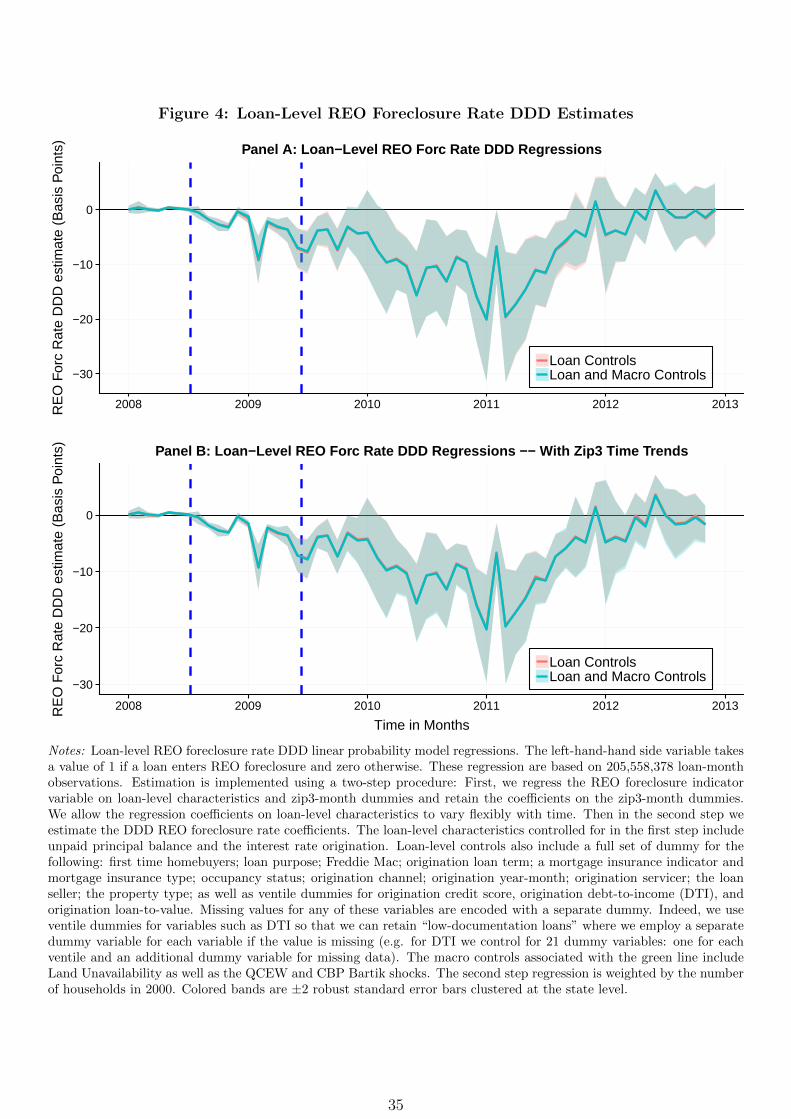
Figure 4: Loan-Level REO Foreclosure Rate DDD Estimates

−30

−20

−10

0

2008 2009 2010 2011 2012 2013RE

O F

orc

Rat

e D

DD

est

imat

e (B

asis

Poi

nts)

Loan ControlsLoan and Macro Controls

Panel A: Loan−Level REO Forc Rate DDD Regressions

−30

−20

−10

0

2008 2009 2010 2011 2012 2013

Time in Months

RE

O F

orc

Rat

e D

DD

est

imat

e (B

asis

Poi

nts)

Loan ControlsLoan and Macro Controls

Panel B: Loan−Level REO Forc Rate DDD Regressions −− With Zip3 Time Trends

Notes: Loan-level REO foreclosure rate DDD linear probability model regressions. The left-hand-hand side variable takesa value of 1 if a loan enters REO foreclosure and zero otherwise. These regression are based on 205,558,378 loan-monthobservations. Estimation is implemented using a two-step procedure: First, we regress the REO foreclosure indicatorvariable on loan-level characteristics and zip3-month dummies and retain the coefficients on the zip3-month dummies.We allow the regression coefficients on loan-level characteristics to vary flexibly with time. Then in the second step weestimate the DDD REO foreclosure rate coefficients. The loan-level characteristics controlled for in the first step includeunpaid principal balance and the interest rate origination. Loan-level controls also include a full set of dummy for thefollowing: first time homebuyers; loan purpose; Freddie Mac; origination loan term; a mortgage insurance indicator andmortgage insurance type; occupancy status; origination channel; origination year-month; origination servicer; the loanseller; the property type; as well as ventile dummies for origination credit score, origination debt-to-income (DTI), andorigination loan-to-value. Missing values for any of these variables are encoded with a separate dummy. Indeed, we useventile dummies for variables such as DTI so that we can retain “low-documentation loans” where we employ a separatedummy variable for each variable if the value is missing (e.g. for DTI we control for 21 dummy variables: one for eachventile and an additional dummy variable for missing data). The macro controls associated with the green line includeLand Unavailability as well as the QCEW and CBP Bartik shocks. The second step regression is weighted by the numberof households in 2000. Colored bands are ±2 robust standard error bars clustered at the state level.

35

Figure 5: Loan-Level Modificaiton Rate DD Estimates

0

5

10

2008 2009 2010 2011 2012 2013

Time in Months

Mod

Rat

e D

D e

stim

ate

(Bas

is P

oint

s)

Loan ControlsLoan and Macro Controls

Panel A: Loan−Level Mod Rate DD Regressions

0

4

8

12

2008 2009 2010 2011 2012 2013

Time in Months

Mod

Rat

e D

D e

stim

ate

(Bas

is P

oint

s)

Loan ControlsLoan and Macro Controls

Panel B: Loan−Level Mod Rate DD Regressions −− With Zip3 Time Trends

Notes: Loan-level modification rate DD linear probability model regressions. The left-hand-hand side variable takesa value of 1 if a loan enters modification and zero otherwise. These regression are based on 206,530,893 loan-monthobservations. For further information on model specification, see the notes to figure 4.

36

Fig

ure

6:

Zip

Code

CF

PL

House

Pri

ceE

stim

ate

s

San

ta B

arba

ra

Sol

ano

Sut

ter

San

Ber

nard

ino

But

te

Col

usa

Con

tra

Cos

ta

Ker

n Los

Ang

eles

Mon

tere

y

Ora

nge

Riv

ersi

de

San

Ben

ito

Son

oma

−30

−20

−10

01020

Pan

el 1

: Med

ian

Syn

thet

ic C

ontro

l Gap

in H

ousi

ng R

etur

ns

OLS

Slo

pe: −

0.02

9 (0

.009

)M

edia

n S

lope

−0.

033

(0.0

03)

−60

−3003060

−50

0−

250

025

0

Syn

thet

ic C

ontr

ol G

ap in

RE

O F

orec

losu

res

Synthetic Control Gap in Housing Returns

Pan

el 2

A: C

FP

L F

orec

losu

re a

nd H

ousi

ng R

etur

n D

DD

Est

imat

es

−5051015

12

34

5

RE

O S

ynth

For

c G

ap Q

uint

ile

Mean House Price Growth

Pan

el 2

B: H

ouse

Pric

e G

row

th b

y C

FP

L R

EO

For

c R

educ

tion

Qui

ntile

s

Notes:

Pan

el1

show

sth

em

edia

nzi

pco

de

leve

lS

ynth

Gap

inh

ouse

pri

cegro

wth

(%)

wit

hin

each

Cali

forn

iaco

unty

from

2008M

07-2

011M

12.

For

each

Cali

forn

iazi

pco

de,

we

con

stru

cta

Synth

etic

Con

trol

usi

ng

the

foll

owin

gva

riab

les

du

rin

gth

ep

re-t

reatm

ent

per

iod

:H

ou

sin

gre

turn

s;R

F2008Q

3fo

recl

osu

rep

red

icti

on

s;2007

un

emp

loym

ent

rate

;2007

hou

seh

old

inco

me;

Lan

dU

nav

aila

bil

ity;

Bar

tik

Sh

ock

s;20

05su

bp

rim

eori

gin

ati

on

rate

;2005

non

-ow

ner

occ

up

ied

ori

gin

ati

on

rate

.V

ari

able

sn

ot

avail

ab

leat

the

zip

cod

ele

vel

are

map

ped

toth

ezi

pco

de

leve

lu

sin

gth

eM

isso

uri

Dat

aB

rid

ge.

Th

eco

unty

nam

esp

rinte

don

the

map

corr

esp

on

dto

those

infi

gu

re2.

Pan

elB

show

sD

DD

OL

San

dM

edia

nre

gres

sion

esti

mat

esof

the

Gap

inh

ouse

pri

cegr

owth

onth

eG

apin

fore

closu

res.

Cou

nty

fore

closu

reG

ap

esti

mate

sare

map

ped

toth

ezi

pco

de

leve

lu

sin

gth

eM

isso

uri

Data

Bri

dge

.R

obu

stO

LS

stan

dar

der

rors

are

clu

ster

edat

the

3-d

igit

zip

cod

ele

vel

an

dro

bu

stqu

anti

lere

gre

ssio

nst

an

dard

erro

rsare

calc

ula

ted

as

sugges

ted

by

Koen

ker

an

dH

all

ock

(200

1).

All

regr

essi

ons

are

wei

ghte

dby

the

nu

mb

erof

hou

seh

old

sin

2000.

Panel

2B

show

sth

esl

op

ees

tim

ate

sfr

om

sep

ara

tere

gre

ssio

ns

of

the

Gap

inh

ou

sep

rice

gro

wth

on

the

Gap

info

recl

osu

res

sep

arat

edby

RE

OS

ynth

Gap

fore

clos

ure

qu

arti

les.

37

Tab

le1:

Th

eIm

pact

of

the

CF

PL

son

Fore

closu

reM

ain

tenance

and

Repair

Cost

s–

Non-J

udic

ial

Sta

tes

Depen

den

tvariable:

For

eclo

sure

Mai

nte

nan

cean

dR

epai

rC

osts

(1)

(2)

(3)

(4)

(5)

(6)

(7)

CA

−57

.887

169.

838

187.

892

(270

.238

)(3

17.5

95)

(281

.653

)

CF

PL

478.

728

229.

776

(172

.828

)(1

78.8

43)

CA×

CF

PL

573.

777

493.

146

471.

543

314.

882

411.

657

946.

176

917.

492

(172

.828

)(1

73.7

95)

(149

.974

)(1

05.0

62)

(106

.468

)(1

84.0

43)

(254

.112

)

Month

sin

RE

O31

4.93

232

4.30

141

2.34

141

1.19

942

0.23

042

3.47

0F

orec

losu

re(4

7.28

8)(4

4.55

4)(6

4.06

8)(6

0.71

8)(6

7.04

5)(6

8.84

2)

Month

sin

RE

O−

3.09

1−

3.35

6−

5.22

2−

5.36

1−

5.68

3−

5.70

9F

orec

losu

re2

(1.3

26)

(1.2

13)

(1.6

82)

(1.6

07)

(1.8

45)

(1.9

12)

Con

stan

t3,

016.

112

1,00

7.34

6(2

70.2

38)

(292

.208

)

RE

OF

orc

Dat

eF

EN

oN

oY

esY

esY

esY

esY

esZ

ip3

FE

No

No

No

Yes

Yes

Yes

Yes

Oth

erL

oan

-lev

elC

ontr

ols

No

No

No

No

Yes

Yes

Yes

Zip

3D

um

mie

s×

Lin

ear

RE

OF

orc

Dat

eT

ren

ds

No

No

No

No

No

Yes

Yes

Zip

3D

um

mie

s×

Qu

ad

rati

cR

EO

Forc

Dat

eT

ren

ds

No

No

No

No

No

No

Yes

Ob

serv

atio

ns

31,0

5631

,056

31,0

5631

,056

31,0

5631

,056

31,0

56

Notes:

Diff

eren

ce-i

n-d

iffer

ence

sre

gres

sion

sof

the

imp

act

ofth

eC

FP

LS

on

fore

closu

rem

ain

ten

ance

an

dre

pair

cost

s.F

ore

closu

res

are

consi

der

edas

inth

ep

re-C

FP

Lp

erio

dif

bot

hth

eR

EO

fore

clos

ure

dat

eand

the

RE

Ofo

recl

osu

red

isp

osit

ion

date

are

bef

ore

the

an

nou

ncm

ent

an

dim

ple

men

tati

on

of

CF

PL

sin

Ju

ly2008.

Fore

closu

res

are

con

sid

ered

inth

eC

FP

Lp

erio

dif

the

RE

Ofo

recl

osu

red

ate

isaf

ter

the

ann

oun

cem

ent

of

the

CF

PL

sin

Ju

ly2008,

bu

tb

efore

the

an

nou

nce

men

tof

HA

MP

inM

arc

h2009.

Thu

s,th

ese

data

incl

ud

en

olo

ans

that

ente

red

into

RE

Ofo

recl

osure

afte

rth

ean

nou

nce

men

tof

HA

MP

.T

he

loan-l

evel

contr

ols

incl

ud

ea

du

mm

yva

riab

lefo

rF

red

die

Mac;

ven

tile

du

mm

ies

for

the

un

pai

dp

rin

cip

alb

alan

ce(o

rigi

nat

ion

and

atfo

recl

osu

re),

bor

row

ercr

edit

score

,th

ed

ebt-

to-i

nco

me

rati

o,

the

ori

gin

ati

on

inte

rest

rate

,an

dlo

an

-to-v

alu

era

tio

at

ori

gin

ati

on;

ind

icat

orva

riab

les

for

occ

up

ancy

stat

us;

and

ind

icat

orva

riab

les

for

the

pu

rpose

of

the

loan

.T

hes

ere

gre

ssio

ns

emp

loy

data

on

lyfr

om

non

-jud

icia

lst

ate

s.T

he

thre

e-d

igit

zip

cod

eti

me

tren

ds

are

zip

cod

ein

dic

ator

sm

ult

ipli

edby

ati

me

tren

dco

rres

pon

din

gto

the

RE

Ofo

recl

osu

red

ate

.R

ob

ust

stan

dard

erro

rsare

clu

ster

edat

the

state

leve

l.

38

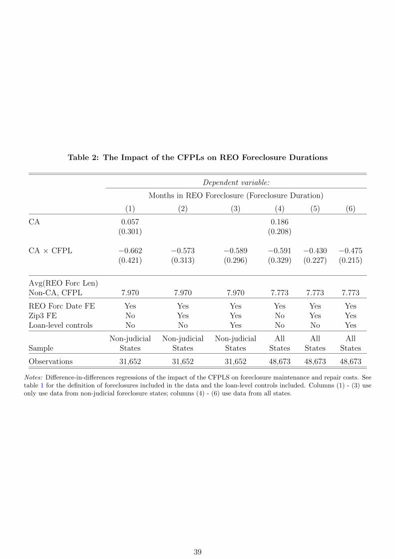
Table 2: The Impact of the CFPLs on REO Foreclosure Durations

Dependent variable:

Months in REO Foreclosure (Foreclosure Duration)

(1) (2) (3) (4) (5) (6)

CA 0.057 0.186(0.301) (0.208)

CA × CFPL −0.662 −0.573 −0.589 −0.591 −0.430 −0.475(0.421) (0.313) (0.296) (0.329) (0.227) (0.215)

Avg(REO Forc Len)Non-CA, CFPL 7.970 7.970 7.970 7.773 7.773 7.773

REO Forc Date FE Yes Yes Yes Yes Yes YesZip3 FE No Yes Yes No Yes YesLoan-level controls No No Yes No No Yes

Non-judicial Non-judicial Non-judicial All All AllSample States States States States States States

Observations 31,652 31,652 31,652 48,673 48,673 48,673

Notes: Difference-in-differences regressions of the impact of the CFPLS on foreclosure maintenance and repair costs. Seetable 1 for the definition of foreclosures included in the data and the loan-level controls included. Columns (1) - (3) useonly use data from non-judicial foreclosure states; columns (4) - (6) use data from all states.

39

Table 3: Probability of Denial and Loan Volume Growth After the CFPLs

Dependent variable:

Prob(Deny) Loan Growth ($) Loan Growth (Num)

(1) (2) (3) (4) (5) (6)

California −0.005 −0.076 0.083 0.077 0.133 0.115(0.013) (0.014) (0.028) (0.026) (0.032) (0.026)

Sample AZ,CA, CA,CO, AZ,CA, CA,CO, AZ,CA, CA,CO,FL,NV NY,TX FL,NV NY,TX FL,NV NY,TX

Loan Level Loan Level Zip Code Zip Code Zip Code Zip Code

Controls? Yes Yes Yes Yes Yes YesEstimation Method LPM LPM OLS OLS OLS OLSObservations 797,732 1,278,510 1,044 1,601 1,044 1,601

Notes: Regressions of the probability of mortgage denial and zip code level loan volume growth on an indicator forCalifornia and controls. In columns (1) and (2), the dependent variable takes a value of one if the mortgage applicationwas denied and zero otherwise and the coefficients from a linear probability model. California takes a value of one forCalifornia and zero otherwise. Controls in columns (1) and (2) include the log of applicant income and loan amount;Zillow house price returns and IRS income and population growth in the year before the loan application was submitted;Land Unavailability; and factor variables for applicant race and applicant sex. The samples include only loans not soldto GSEs in AZ, CA, FL, and NV (column 1) and CA, CO, NY, and TX (column 2) from 2009 to 2014. Columns (3) -(4) and (5) - (6) show regressions where dollar loan volume growth or the growth in the number of loans represents thedependent variable. Loan volume growth is defined as (ln(Loan vol2009 + · · ·+ Loan vol2014))− (ln(Loan vol2007)). Thesample is restricted to loans not sold to GSEs. The key right-hand-side variable of interest is an indicator that takes avalue of one for California. The data for these regressions are at the zip code level. Controls include Land Unavailability,applicant income growth and IRS income and population growth as well as Zillow zip code level house price growth for2008-2009, 2010-2011, and 2012-2014. The regressions in columns (3) - (6) are weighted by the number of households.Robust standard errors are clustered at the 3-digit zip code level.

40

A Online Appendix: The California Foreclosure Prevention Laws

SB-1137:California Senate Bill 1137 (SB-1137) was passed and implemented on July 8, 2008 and mandated

that mortgage lenders operating in California delay filing an NOD until 30 days after contacting thehomeowner with information on foreclosure alternatives.18 Specifically, SB-1137 required the lender tocontact the borrower in person or over the telephone and notify the borrower of his right to schedulea meeting with the lender to discuss foreclosure alternatives. The mortgagor then had the right toschedule a meeting with the lender within 14 days of first contact. Then, after the initial contact orattempted “due diligence”, the law required the lender to wait 30 days before filing an NOD. Threeattempts to contact the mortgagor over the telephone on different days and at different times satisfiedthe law’s due diligence requirement. This due diligence requirement likely created large foreclosureinstitutional costs for lenders as many lacked the infrastructure to contact borrowers by telephone ona large scale (Agarwal et al., 2017). Further, the law required the legal owner who took possession of avacant residential property via foreclosure to maintain it or face fines of up to $1000 per property perday.19 The sunset date for SB-1137 was January 1, 2013.

Prior to the enactment of SB-1137, existing law only required that the lender file an NOD with theappropriate county recorder and then mail the NOD to the mortgage borrower. In sending the NOD,lenders were not obligated to provide information on foreclosure alternatives. The aim of SB-1137 wasto alert struggling homeowners of foreclosure alternatives via mortgage lenders and change the netpresent value calculation of foreclosure versus mortgage modification.20

The California Foreclosure Prevention Act (CFPA):The CFPA was signed into law on February 20, 2009 and went into effect on June 15, 2009 for

the period extending through January 1, 2011. The aim of the CFPA was to provide lenders withincentives to implement comprehensive mortgage modification programs during a period of housingcrisis and widespread mortgage failure. The CFPA prohibited lenders from issuing an NOS for anadditional 90 days after the initial NOD unless the lender enacted a mortgage modification programmeeting the requirements of CFPA. As a non-judicial foreclosure state, California already required athree month waiting period between the NOD and the NOS. Thus, under the CFPA, lenders thathad not implemented comprehensive loan modification programs meeting the CFPA regulations wererequired to wait a total of six months between the NOD and the NOS.

Mortgage lenders who implemented an acceptable mortgage modification program were exemptedfrom the additional 90 day CFPA foreclosure moratorium. To obtain this exemption, a lender’s loanmodification program was required to achieve affordability and sustainability targets for modifiedloans.21

To be eligible for a mortgage modification under the CFPA a borrower must (1) live in the property;(2) be in default (foreclosure); (3) document an ability to pay the modified loan; (4) have obtained themortgage under consideration between January 1, 2003 to January 1, 2008; and (5) not have surrenderedthe property or engaged in a bankruptcy proceeding. The CFPA also required that mortgages underconsideration for modification be the first lien on a property in California. All loans originated inCalifornia that meet the above requirements were subject to the provisions of the CFPA. Loans wherea servicing or pooling agreement prohibited modification are exempt from the CFPA. The State ofCalifornia also outlined a number of procedures related to the implementation of the CFPA. When amortgage lender submitted an application for exemption under the CFPA, the State immediately issueda temporary order of exemption from the CFPA foreclosure moratorium. Then, within 30 days, thelender received a final notification of exemption or denial regarding the mortgage modification program.

An adequate CFPA modification program was required to keep borrowers in their homes when the

18http://leginfo.legislature.ca.gov/faces/billNavClient.xhtml?bill_id=200720080SB113719Further, SB-1137 was only applicable for mortgages on owner-occupied homes originated between January 1, 2003

and December 31, 2007.20Indeed, the Bill’s chaptered text cites a Freddie Mac report that suggested that 57 percent of late paying borrowers

did not know that their lender may offer a foreclosure alternative.21Note that lenders participating in the HAMP program were considered to be in compliance with the CFPA and thus

were exempt from the extra 90 day foreclosure moratorium under the law.

41

anticipated recovery under the loan modification or workout exceeded the proceeds from foreclosure ona net present value basis. Mortgage modification programs were also mandated to achieve a housing-related debt to gross income ratio of 38 percent or less on an aggregate basis and contain at leasttwo of the following features: An interest rate reduction over a fixed term for a minimum of fiveyears; an extension of the loan amortization period up to 40 years from the original date of the loan;deferral of principal until the maturity of the loan; a reduction in principal; compliance with a federalgovernment mortgage program; or other factors that the state Commissioner deemed appropriate. TheCFPA also outlined long-term sustainability goals regarding the performance of mortgage loans modifiedunder the CFPA. In particular, the CFPA guidelines state that a modified loan was sustainable if theborrower’s monthly payment under the modified loan was reduced for five years; if the modificationyielded a housing-related debt-to-income ratio of at most 38 percent; if the borrower’s back-end debt-to-income ratio was no more than 55 percent (the back-end debt-to-income ratio is the total monthlydebt expense divided by gross monthly income); if under the modified loan, the borrower was currenton his mortgage after a three month period; or if the modification satisfied the requirements of a federalprogram. Applicants filing for an exemption via HAMP may have been required to submit a copy oftheir Servicer Participation Agreement for HAMP under the Emergency Economic Stabilization Act of2008.

The CFPA was signed into law on February 20, 2009 and went into effect on June 15, 2009 for theperiod extending through January 1, 2011. In March 2009, California established a timeline for theimplementation of the CFPA and posted it online; on April 21, 2009 the CA government released adraft of the emergency regulations to interested parties and accepted comments until May 6, 2009; OnMay 21, 2009, the emergency regulations associated with the CFPA were filed with the California Officeof Administrative Law (OAL); and on June 1, 2009, the OAL approved the emergency regulations andfiled them with the Secretary of State.

In total, 149 applications were submitted for exemptions from the CFPA foreclosure moratorium.Of these 149 applications, 78.5 percent were accepted, 11.5 percent were denied, and 10 percent ofthe applications were withdrawn. Hence, a non-trivial portion of the submitted mortgage modificationprograms did not meet the CFPA standards. Note also that the number of applications for the CFPAexemption was lower than anticipated as some lenders preferred the additional 90 days in foreclosure sothey could avoid taking possession of non-performing properties at the height of the crisis (California,2010).

42

B Online Appendix: State Synthetic Control Results

Table B1: State-Level Synthetic Control Estimation Results

CFPL Treatment Period

Pre GapMSE CA Synth Gap Pcntle(1) (2) (3) (4) (5)

Panel A: Foreclosures and the MDRI

Forc Starts (% of All Loans) 0.01 20.90 32.81 -11.91 0.00Prime Forc Starts (% of Prime Loans) 0.00 17.26 29.08 -11.82 0.00Subprime Forc Starts (% of Subprime Loans) 0.03 59.18 83.40 -24.22 0.00Zillow REO Forc per 10,000 Homes 0.95 839.71 1208.86 -369.15 0.00Mortgage Default Risk (MDRI) 0.01 25.47 53.52 -28.04 0.00

Panel B: House Price Growth

FHFA HP Growth (%) 0.40 -25.25 -47.94 22.69 100.00Zillow All Homes HP Growth (%) 0.03 -28.48 -46.01 17.53 100.00Zillow Bottom Tier HP Growth (%) 0.05 -47.67 -70.98 23.31 100.00Zillow Top Tier HP Growth (%) 0.04 -13.56 -23.34 9.78 91.18

Notes: The far left column lists the outcome variable, Pre-MSE in column (1) is the mean-squared error from theSynthetic control match during the pre-treatment period (2004M01-2008M06), the next two columns (2 & 3) show thechange in the outcome variable for California and its Synthetic Control during the CFPL treatment period, and Gap incolumn (4) is the difference between of the change in the outcome variable for treated unit (California) relative to itsSynthetic Control. The MDRI over the treatment period is the cumulative sum in its index points over the treatmentperiod. Column (5) shows the percentile of the Gap estimate relative to all placebo effects. This is calculated by firstestimating the empirical CDF from all placebo effects and then calculating the percentile of the Gap for California relativeto the CDF of placebo effects. The treatment period ranges from 2008M07 to 2011M12. The variable descriptions anddata sources are in the notes to figure 1 and in appendix C.

43

C Online Appendix: Data List

Variable Source

State Level Data

Foreclosure Starts (Notice of Default); (% of All Loans) Mortgage Bankers’ AssocPrime Forc Starts (% of Prime Loans) Mortgage Bankers’ AssocSubprime Forc Starts (% of Subprime Loans) Mortgage Bankers’ AssocZillow REO Foreclosures per 10,000 Homes ZillowMortgage Default Risk (MDRI) Chauvet et al. (2016)FHFA All Transaction House Price Returns FHFAZillow All Homes Returns ZillowZillow Bottom Tier Returns ZillowZillow Top Tier Returns Zillow

County Level Data

Zillow REO Foreclosures per 10,000 Homes ZillowZillow All Homes Returns ZillowUnemployment Rate BLSLand Unavailability Lutz and Sand (2017)Bartik Labor Demand Shocks Compiled From County Business PatternsBartik Labor Demand Shocks Compiled From BLS QCEWMaximum Unemployment Benefits Hsu et al. (2018) (State)Income Per Household, 2007 IRS Statistics of Income% of Subprime Mortgage Loans, 2005 HMDA & HUD Subprime ListNon-Occupied Occupation Rate (NonOccRate), 2005 HMDA & Gao et al. (2017)

Zip Code Level Data

Zillow All Homes Returns ZillowUnemployment Rate BLS (county level)Land Unavailability Lutz and Sand (2017)Bartik Labor Demand Shock Compiled From CBP (County)Maximum Unemployment Benefits Hsu et al. (2018) (State)Income Per Household, 2007 IRS Statistics of Income% of Subprime Mortgage Loans, 2005 HMDA & HUD Subprime ListNon-Occupied Occupation Rate (NonOccRate), 2005 HMDA & Gao et al. (2017)

Loan Level Data

GSE Loan Performance Fannie Mae & Freddie MacHome Mortgage Disclosure Act (HMDA) FFIEC

44

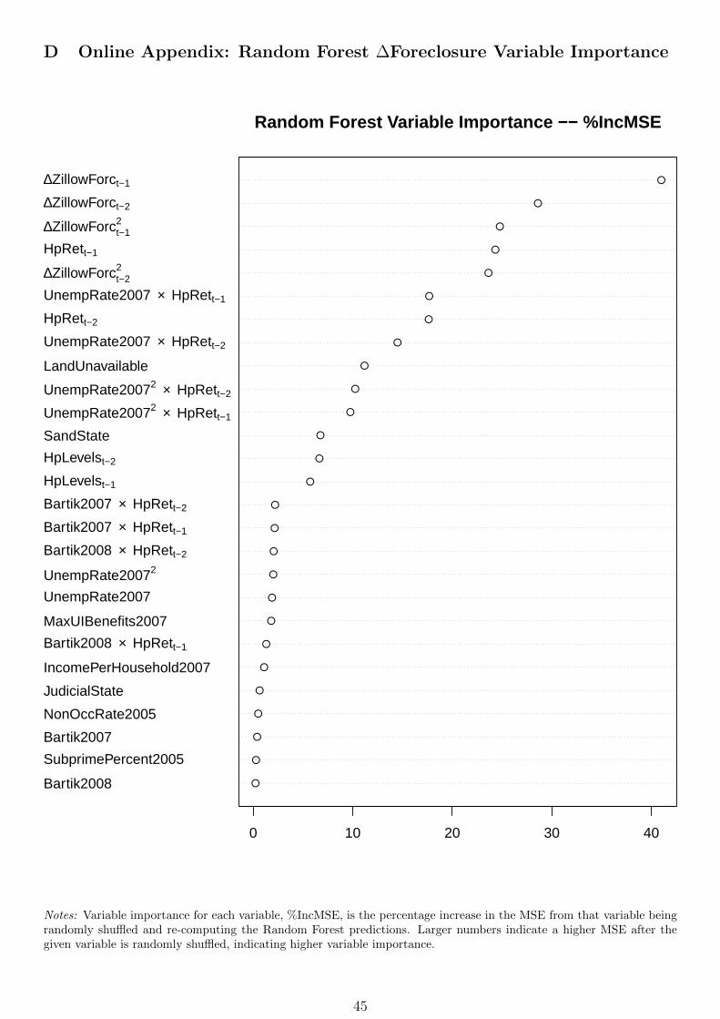
D Online Appendix: Random Forest ∆Foreclosure Variable Importance

Bartik2008

SubprimePercent2005

Bartik2007

NonOccRate2005

JudicialState

IncomePerHousehold2007

Bartik2008 × HpRett−1

MaxUIBenefits2007

UnempRate2007

UnempRate20072

Bartik2008 × HpRett−2

Bartik2007 × HpRett−1

Bartik2007 × HpRett−2

HpLevelst−1

HpLevelst−2

SandState

UnempRate20072 × HpRett−1

UnempRate20072 × HpRett−2

LandUnavailable

UnempRate2007 × HpRett−2

HpRett−2

UnempRate2007 × HpRett−1

∆ZillowForct−22

HpRett−1

∆ZillowForct−12

∆ZillowForct−2

∆ZillowForct−1

●

●

●

●

●

●

●

●

●

●

●

●

●

●

●

●

●

●

●

●

●

●

●

●

●

●

●

0 10 20 30 40

Random Forest Variable Importance −− %IncMSE

Notes: Variable importance for each variable, %IncMSE, is the percentage increase in the MSE from that variable beingrandomly shuffled and re-computing the Random Forest predictions. Larger numbers indicate a higher MSE after thegiven variable is randomly shuffled, indicating higher variable importance.

45

E Online Appendix: Loan-level Foreclosure Alternate Rate DDD Esti-mates

Figure 7: Loan-Level Foreclosure Alternate Rate DDD Estimates

−40

−30

−20

−10

0

2008 2009 2010 2011 2012 2013

Time in Months

For

c A

lt D

DD

est

imat

e (B

asis

Poi

nts)

Loan ControlsLoan and Macro Controls

Panel A: Loan−Level Forc Alt Rate DDD Regressions

−30

−20

−10

0

10

2008 2009 2010 2011 2012 2013

Time in Months

For

c A

lt D

DD

est

imat

e (B

asis

Poi

nts)

Loan ControlsLoan and Macro Controls

Panel B: Loan−Level Forc Alt Rate DDD Regressions −− With Zip3 Time Trends

Notes: Loan-level foreclosure alternate rate DDD linear probability model regressions. The left-hand-hand side variabletakes a value of 1 if a loan becomes a foreclosure alternate (Short Sale, Third Party Sale, Charge Off, Note Sale) andzero otherwise. For further information on model specification, see the notes to figure 4.

F Online Appendix: CFPLS and Maintenance Costs – All States

46

Tab

leA

1:

Th

eIm

pact

of

the

CF

PL

son

Fore

closu

reM

ain

tenance

and

Repair

Cost

s–

All

Sta

tes

Depen

den

tvariable:

For

eclo

sure

Mai

nte

nan

cean

dR

epai

rC

osts

(1)

(2)

(3)

(4)

(5)

(6)

(7)

CA

−56

.529

105.

762

154.

533

(160

.125

)(1

93.1

03)

(172

.979

)

CF

PL

518.

554

227.

229

(115

.278

)(1

15.3

37)

CA×

CF

PL

533.

950

475.

247

423.

616

262.

886

338.

503

919.

915

838.

276

(115

.278

)(1

12.7

01)

(100

.301

)(8

1.24

6)(8

5.97

6)(1

35.3

88)

(188

.824

)

Mon

ths

inR

EO

328.

373

334.

543

412.

282

407.

824

413.

435

416.

606

Fore

clos

ure

(41.

607)

(41.

094)

(44.

527)

(41.

949)

(45.

949)

(46.

996)

Mon

ths

inR

EO

−2.

967

−3.

145

−4.

909

−4.

927

−5.

105

−5.

129

For

eclo

sure

2(1

.083

)(1

.045

)(1

.230

)(1

.186

)(1

.337

)(1

.387

)

Con

stan

t3,

014.

754

984.

459

(160

.125

)(1

96.5

14)

RE

OF

orc

Dat

eF

EN

oN

oY

esY

esY

esY

esY

esZ

ip3

FE

No

No

No

Yes

Yes

Yes

Yes

Oth

erL

oan

-lev

elC

ontr

ols

No

No

No

No

Yes

Yes

Yes

Zip

3D

um

mie

s×

Lin

ear

RE

OF

orc

Dat

eT

ren

ds

No

No

No

No

No

Yes

Yes

Zip

3D

um

mie

s×

Qu

ad

rati

cR

EO

Forc

Dat

eT

rend

sN

oN

oN

oN

oN

oN

oY

es

Ob

serv

ati

on

s47

,887

47,8

8747

,887

47,8

8747

,887

47,8

8747

,887

Notes:

See

the

note

sfo

rta

ble

1.

Th

ista

ble

use

sd

ata

from

all

state

s.

47

G Online Appendix: CFPL Zip Code House Price Growth Estimates

Table G1: Zip Code CFPL DDD Regressions – Foreclosures and House Price Growth

Dep Var : Synth Gap in Housing Returns

OLS Median Reg

(1) (2) (3) (4)

Synthetic Control −0.029 −0.028 −0.033 −0.038Gap in Foreclosures (0.009) (0.009) (0.003) (0.004)

Bartik Shock −0.318 1.2052009 - 2011 (1.535) (0.737)

Household Income −0.068 −0.061in 2007 ($000s) (0.021) (0.018)

House Price ($000s) 0.021 0.017(0.005) (0.003)

Constant −1.349 −9.402 −0.794 2.417(1.715) (11.904) (0.739) (5.825)

Observations 1,079 1,079 1,079 1,079R2 0.101 0.162

Notes: Regressions are weighted by the number of households in 2000. For OLS, robust standard errors are clusteredat the three digit zip code level. For quantile median regression estimates, standard errors are computed using a robustHuber sandwich esimtate as suggested by Koenker and Hallock (2001).

48