A coupled CFD-FEM strategy to predict thermal fatigue in mixing tees of nuclear reactors

M.H.C. Hannink, A.K. Kuczaj, F.J. Blom, J.M. Church and E.M.J. Komen

Safety & Performance Nuclear Research and Consultancy Group (NRG) P.O. Box 25, 1755 ZG Petten, The Netherlands

hannink@nrg.eu

Abstract:

Fluctuating stresses imposed on a piping system are potential causes of thermal fatigue failures in energy cooling systems of nuclear power plants [4]. These stresses are generated due to temperature fluctuations in regions where cold and hot flows are intensively mixed together. A typical situation for such mixing appears in turbulent flow through a T-junction. In the present work, turbulent mixing in a T-junction is investigated by a coupled approach of fluid-flow calculations and mechanical calculations. The flow characteristics and the temperatures in the pipe wall are obtained using Large-Eddy Simulations (LES). The corresponding structural stresses, causing the fatigue loading, are determined by means of finite element calculations. In general, LES is very well capable of capturing the mixing phenomena and the accompanied turbulent flow fluctuations in a T-junction. Previous work based on a direct comparison with experimental results [8, 9] showed the accuracy of LES predictions for thermal fatigue assessment in case of adiabatic flow. In this paper, also the effect of heat transfer through the pipe walls is included in the simulations. Temperatures are solved in both fluid and structure. Subsequently, the temperatures in the structure are transferred from the fluid-flow model to the finite element model. Using the finite element method, a mechanical calculation is performed to determine the structural deformations and stresses due to these thermal loads. Based on the resulting stresses, the fatigue life of the T-junction is finally predicted using fatigue curves from a design code. A strategy has been developed to assess thermal fatigue of complex mixing problems in nuclear power plants by coupling LES modelling, finite element modelling and code assessment. A description of this approach along with its application to a specified test case is presented here.

1 INTRODUCTION Thermal fatigue is a safety related issue in primary pipework systems of nuclear power plants. Especially, due to the life extension of current reactors and the design of a next generation of new reactors, this is an issue of growing importance. The thermal fatigue degradation mechanism is induced by temperature fluctuations in a fluid, which arise when hot and cold flows are mixed. Possible phenomena that can occur are, e.g., thermal stratification, thermal striping, and turbulent mixing [5]. Currently, most of these common thermal fatigue issues are well understood and can be monitored by plant instrumentation systems at fatigue susceptible locations [5, 10]. However, high-cycle temperature fluctuations associated with turbulent mixing cannot be adequately detected by common thermocouple instrumentations. For a proper evaluation of thermal fatigue, therefore, numerical simulations are necessary. In this paper, a strategy for the numerical prediction of thermal fatigue is presented.

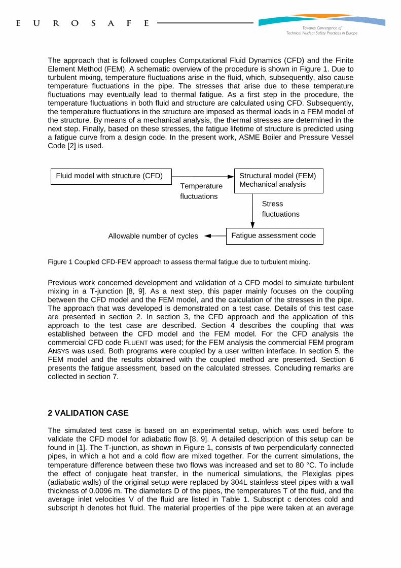
The approach that is followed couples Computational Fluid Dynamics (CFD) and the Finite Element Method (FEM). A schematic overview of the procedure is shown in Figure 1. Due to turbulent mixing, temperature fluctuations arise in the fluid, which, subsequently, also cause temperature fluctuations in the pipe. The stresses that arise due to these temperature fluctuations may eventually lead to thermal fatigue. As a first step in the procedure, the temperature fluctuations in both fluid and structure are calculated using CFD. Subsequently, the temperature fluctuations in the structure are imposed as thermal loads in a FEM model of the structure. By means of a mechanical analysis, the thermal stresses are determined in the next step. Finally, based on these stresses, the fatigue lifetime of structure is predicted using a fatigue curve from a design code. In the present work, ASME Boiler and Pressure Vessel Code [2] is used.

Figure 1 Coupled CFD-FEM approach to assess thermal fatigue due to turbulent mixing.

Previous work concerned development and validation of a CFD model to simulate turbulent mixing in a T-junction [8, 9]. As a next step, this paper mainly focuses on the coupling between the CFD model and the FEM model, and the calculation of the stresses in the pipe. The approach that was developed is demonstrated on a test case. Details of this test case are presented in section 2. In section 3, the CFD approach and the application of this approach to the test case are described. Section 4 describes the coupling that was established between the CFD model and the FEM model. For the CFD analysis the commercial CFD code FLUENT was used; for the FEM analysis the commercial FEM program ANSYS was used. Both programs were coupled by a user written interface. In section 5, the FEM model and the results obtained with the coupled method are presented. Section 6 presents the fatigue assessment, based on the calculated stresses. Concluding remarks are collected in section 7.

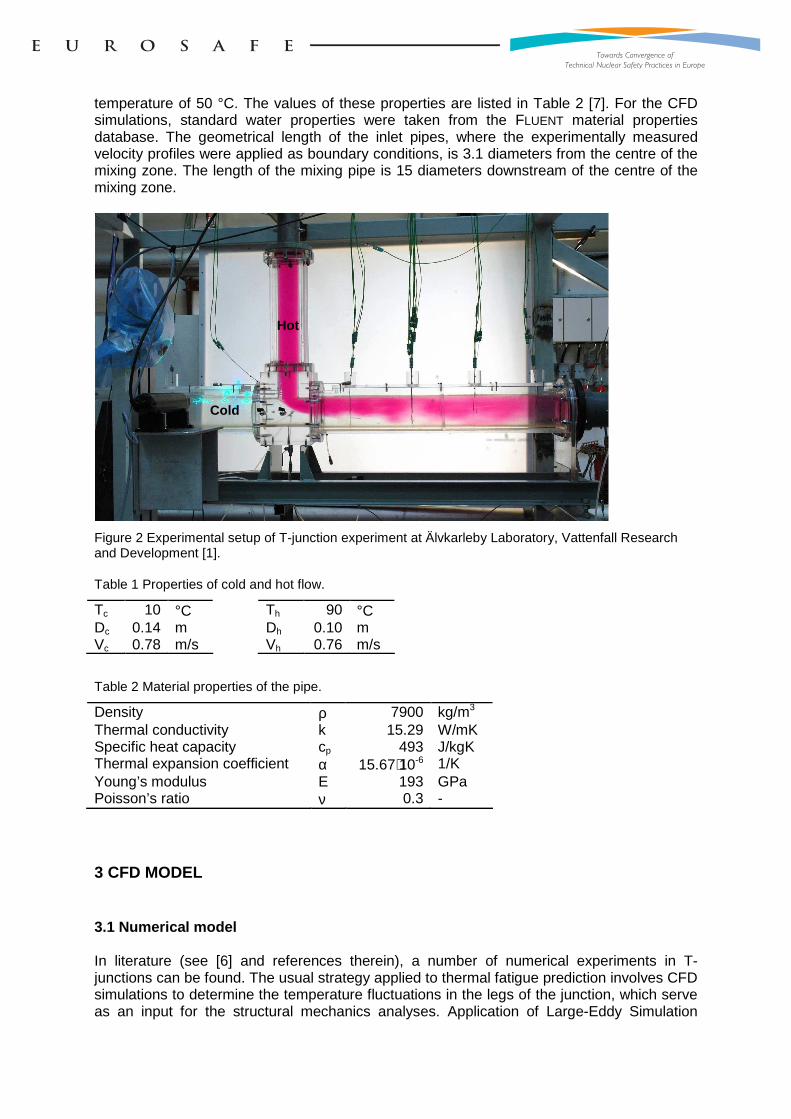
2 VALIDATION CASE The simulated test case is based on an experimental setup, which was used before to validate the CFD model for adiabatic flow [8, 9]. A detailed description of this setup can be found in [1]. The T-junction, as shown in Figure 1, consists of two perpendicularly connected pipes, in which a hot and a cold flow are mixed together. For the current simulations, the temperature difference between these two flows was increased and set to 80 °C. To include the effect of conjugate heat transfer, in the numerical simulations, the Plexiglas pipes (adiabatic walls) of the original setup were replaced by 304L stainless steel pipes with a wall thickness of 0.0096 m. The diameters D of the pipes, the temperatures T of the fluid, and the average inlet velocities V of the fluid are listed in Table 1. Subscript c denotes cold and subscript h denotes hot fluid. The material properties of the pipe were taken at an average

Structural model (FEM) Mechanical analysis

Fluid model with structure (CFD) Temperature fluctuations

Fatigue assessment code Allowable number of cycles

Stress fluctuations

temperature of 50 °C. The values of these properties are listed in Table 2 [7]. For the CFD simulations, standard water properties were taken from the FLUENT material properties database. The geometrical length of the inlet pipes, where the experimentally measured velocity profiles were applied as boundary conditions, is 3.1 diameters from the centre of the mixing zone. The length of the mixing pipe is 15 diameters downstream of the centre of the mixing zone.

Figure 2 Experimental setup of T-junction experiment at Älvkarleby Laboratory, Vattenfall Research and Development [1].

Table 1 Properties of cold and hot flow.

Tc 10 °C Th 90 °C Dc 0.14 m Dh 0.10 m Vc 0.78 m/s Vh 0.76 m/s

Table 2 Material properties of the pipe.

Density ρ 7900 kg/m3

Thermal conductivity k 15.29 W/mK Specific heat capacity cp 493 J/kgK Thermal expansion coefficient α 15.67⋅10-6 1/K Young’s modulus E 193 GPa Poisson’s ratio ν 0.3 -

3 CFD MODEL

3.1 Numerical model In literature (see [6] and references therein), a number of numerical experiments in T-junctions can be found. The usual strategy applied to thermal fatigue prediction involves CFD simulations to determine the temperature fluctuations in the legs of the junction, which serve as an input for the structural mechanics analyses. Application of Large-Eddy Simulation

Hot

Cold

(LES) methods allows partially resolving flow scales at computationally acceptable costs. Accurate LES predictions require considerably high computational effort due to a number of scales that need to be resolved. In [8, 9] an assessment of LES validity for simulation of turbulent mixing in a T-junction was presented in detail. In this paper, we used a similar computational setup with slight modifications that will be described momentarily. In the present work, a structure is included and simulations are performed with conjugate heat transfer, which allows interchanging heat at the wall between fluid and solid. We concentrate on the numerical analysis of the damping effect introduced by the structure due to the difference in conductivity between fluid and solid. Such an analysis is helpful in determination of important flow time-scales, which have an impact on the thermal characteristics in a solid. This will be presented in section 4.2. For the current simulations we used the commercial CFD package FLUENT with a second order implicit non-iterative time-advancement scheme. Wall-adapting local eddy-viscosity (WALE) model was used for LES. For convective terms in the momentum equation, bounded central differencing was used with a second order upwind scheme for the energy equation and a standard PISO algorithm for coupling pressure and velocity. The initial condition was taken from a well-developed case in which a few flow cycles (7 s) were simulated without recording the data statistics. Subsequently, simulations were performed for 6 s of the physical time with a time-step of 0.001 s. This is approximately more than two cycle times when the inlet flow reaches the outlet. For the final structural analyses only 2.5 s of the flow statistics was taken. Obviously, this time is too short for a proper fatigue assessment but sufficient for the demonstration case presented here. Data were recorded with a frequency of 0.005 s, which will be justified in the next section. The boundary conditions were identical to the boundary conditions of the simulations presented in [8, 9], apart from the outer wall conditions for the solid. In this case, adiabatic (zero-heat flux) conditions were used.

3.2 CFD results In this section we concentrate on the flow characteristics present in the T-junction. To visualise the important physical phenomena associated with turbulent mixing, two snapshots of the fluid velocity and temperature field are presented. A more quantitative description can be found in [8, 9]. In Figure 3 the magnitude of the velocity field is presented. Two fluid streams accelerate in the mixing zone and together they form a jet-like structure, which has a recirculation zone in the upper part of the downstream pipe. Further downstream, turbulent flow is observed with a high flow variability, which mixes hot and cold fluid streams. In Figure 4 the temperature field is presented. In the mixing zone, areas of hot and cold fluid can be distinguished, that are mixed further downstream.

Figure 3 Magnitude of fluid velocity at t = 3 s.

Figure 4 Fluid temperature at t = 3 s.

4 CFD-FEM COUPLING

4.1 Coupling To calculate the stresses that are induced in the pipe by the temperature fluctuations in the fluid, coupling was established between the CFD model and the FEM model. The structural temperatures resulting from the CFD analysis were used as thermal loads in the FEM analysis. The current implementation of export procedures in FLUENT does not allow directly exporting the results obtained in the structure to an ANSYS input file in a satisfactory way. Therefore, a user written interface was created between FLUENT and ANSYS. For the fatigue assessment, mainly the fluctuations of the stresses are of interest. One way to determine these fluctuations is to calculate them after the mechanical analysis is performed. Since the mechanical analysis is linear, the stress fluctuations can also be obtained directly by using temperature fluctuations as thermal loads in the FEM model. For the simulations presented here, the last option was chosen because it provides a more direct insight into the relation between the stress fluctuations and the temperature fluctuations, which cause the fatigue. The temperature fluctuation at a certain position and time is defined

here as the difference between the temperature at this position and time, and the time-averaged temperature at this position1. Since the structural mesh of the CFD model and the FEM model were coincident, no mapping had to be used to transfer data. Both temperatures exported from FLUENT and imported in ANSYS were nodal values. To establish coupling, the following steps were performed: � Exporting nodal temperatures of the structure from FLUENT; � Calculating time averaged nodal temperatures of the structure; � Calculating nodal temperature fluctuations of the structure; � Finding the corresponding nodes in ANSYS; � Writing an ANSYS input file to impose temperature fluctuations as thermal loads at the

nodes. In previous work on the coupled CFD-FEM method [3], inaccuracies introduced by FLUENT export procedures in the interpolation of cell centred temperatures in the fluid to nodal temperatures at the interface were discovered. Figure 5 shows the temperature fluctuations through the wall that result from the current simulations. The temperature profile is a smooth curve, which means that the mesh of the structure is fine enough to describe the penetration of the temperature fluctuations in the pipe wall properly. Before the calculations, the size of the cells/elements was estimated using penetration theory. Furthermore, it can be seen that the temperature fluctuations at the interface are in line with the temperature fluctuations in the rest of the wall. This means that no interpolation error is encountered and coupling works properly.

Figure 5 Temperature fluctuations through the pipe wall at t = 1.300 s and x = 0.172 m.

4.2 Simulation time In order to supply the important input for the structural mechanics simulations, we may ask what is the minimal frequency at which we need to record data in order to capture the relevant temperature variations that may cause damage. To investigate this issue, we recorded temperature at various positions at the wall (facet average from the nearest computational cell wall), in the fluid and the solid. In Figure 6 the temperatures recorded in 1 This definition differs from the mean-square fluctuation that is equivalent to the variance, i.e., a mathematical expectation of the average squared deviation from the mean. However, this remark was included just for consistency as it does not have any influence on the performed analysis.

A

A

the fluid and the solid are shown for two numerical sensors, localised at approximately 3.6 and 6.6 diameters downstream of the mixing zone. It is important to realise that fluid and solid are coupled through the heat flux (mathematically in the energy equation), but due to different conductivities of these two media, the actual temperature fluctuations significantly differ from each other in the near vicinity of walls. The amplitudes of the temperature fluctuations in the solid (pipe) are significantly lower than in the fluid. However, the frequency contents of these two signals are nearly the same (see Figure 7). Having these two signals in the Fourier domain, we can easily perform filtering by cutting-off the Fourier modes above a specified frequency to examine the importance of higher frequencies. As we may see from the spectrum, the high-frequency modes have very small amplitudes, thus they do not contribute significantly to the relevant fluctuations. In fact, after filtering the results with a cutoff of 10 Hz and transforming the signals back to the time-domain we see that they still preserve their original shape (see Figure 8). In this way we can estimate the smallest recording time needed to capture the relevant temperature fluctuations at the wall, which can be larger than the time-step in CFD simulations, since the latter must capture the small-scale ‘events’ generated by turbulence in the fluid. For the current demonstration case, a recording interval of 0.005 s (200 Hz) was chosen, which is more than enough to resolve all the important temperature variations in the fluid. A frequency of the order of 50 Hz (recording interval of 0.020 s) would be sufficient to capture important amplitudes below 25 Hz, assuming a factor of two for the aliasing error. This will be also shown later in the paper.

(a) (b)

Figure 6 Temperature in fluid and solid as a function of time, 3.6 diameters (z = 0.1 m, y = 0) (a) and 6.6 diameters (y = 0.1 m, z = 0) (b) downstream in the T-junction.

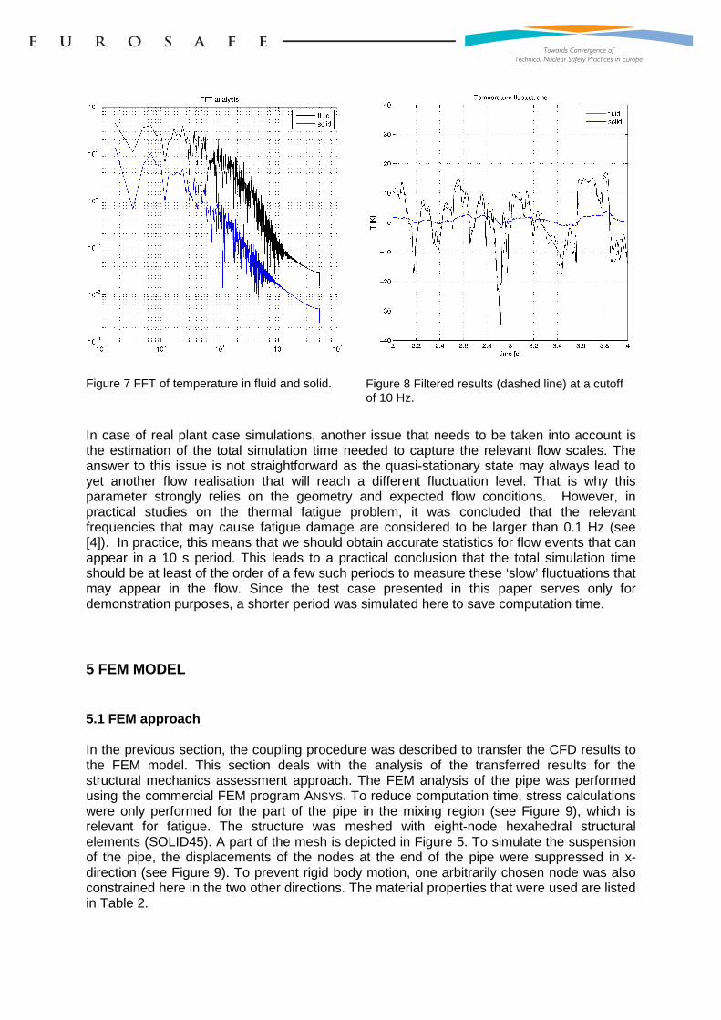
Figure 7 FFT of temperature in fluid and solid.

Figure 8 Filtered results (dashed line) at a cutoff of 10 Hz.

In case of real plant case simulations, another issue that needs to be taken into account is the estimation of the total simulation time needed to capture the relevant flow scales. The answer to this issue is not straightforward as the quasi-stationary state may always lead to yet another flow realisation that will reach a different fluctuation level. That is why this parameter strongly relies on the geometry and expected flow conditions. However, in practical studies on the thermal fatigue problem, it was concluded that the relevant frequencies that may cause fatigue damage are considered to be larger than 0.1 Hz (see [4]). In practice, this means that we should obtain accurate statistics for flow events that can appear in a 10 s period. This leads to a practical conclusion that the total simulation time should be at least of the order of a few such periods to measure these ‘slow’ fluctuations that may appear in the flow. Since the test case presented in this paper serves only for demonstration purposes, a shorter period was simulated here to save computation time.

5 FEM MODEL

5.1 FEM approach In the previous section, the coupling procedure was described to transfer the CFD results to the FEM model. This section deals with the analysis of the transferred results for the structural mechanics assessment approach. The FEM analysis of the pipe was performed using the commercial FEM program ANSYS. To reduce computation time, stress calculations were only performed for the part of the pipe in the mixing region (see Figure 9), which is relevant for fatigue. The structure was meshed with eight-node hexahedral structural elements (SOLID45). A part of the mesh is depicted in Figure 5. To simulate the suspension of the pipe, the displacements of the nodes at the end of the pipe were suppressed in x-direction (see Figure 9). To prevent rigid body motion, one arbitrarily chosen node was also constrained here in the two other directions. The material properties that were used are listed in Table 2.

Figure 9 Geometry of test case for mechanical analysis.

For each time step, a steady-state mechanical analysis was performed, where the temperature fluctuations resulting from the CFD calculations were imposed as thermal loads at the nodes. The CFD results were recorded with a time step of 0.005 s, which was proven to be sufficient in the previous section. In Figure 12 it is shown that, to capture the variation of the temperature fluctuations in the structure, even a larger time step can be used. The stress calculations were therefore performed with a time step of 0.020 s. For demonstration purposes, a total simulation time was chosen of 2.5 s (see also section 3.1).

5.2 FEM results

5.2.1 Temperature fluctuations In this section, the analysis of the temperature fluctuations is presented. For the simulated time interval, the temperature field was time-averaged at every location in the pipe and the fluctuations were measured with respect to these time-averaged values. Figure 10 shows two examples of temperature fluctuations in the pipe, which were used as thermal loads in the FEM model. Since the highest temperature fluctuations occur at the inner wall of the pipe, this is the most interesting part for the fatigue assessment. In the beginning of the mixing region, hot and cold spots are observed, which travel through the pipe with the velocity of the fluid. Similar spots were identified by Blom et al. [12] in the numerical simulations of experiments performed in the Fatherino 2 facility.

Figure 10 Temperature fluctuations at the inner pipe wall at two different times.

x

z

0.10

1.10

0.14

0.10

Mechanical analysis Suspension

t = 1.645 s t = 1.805 s

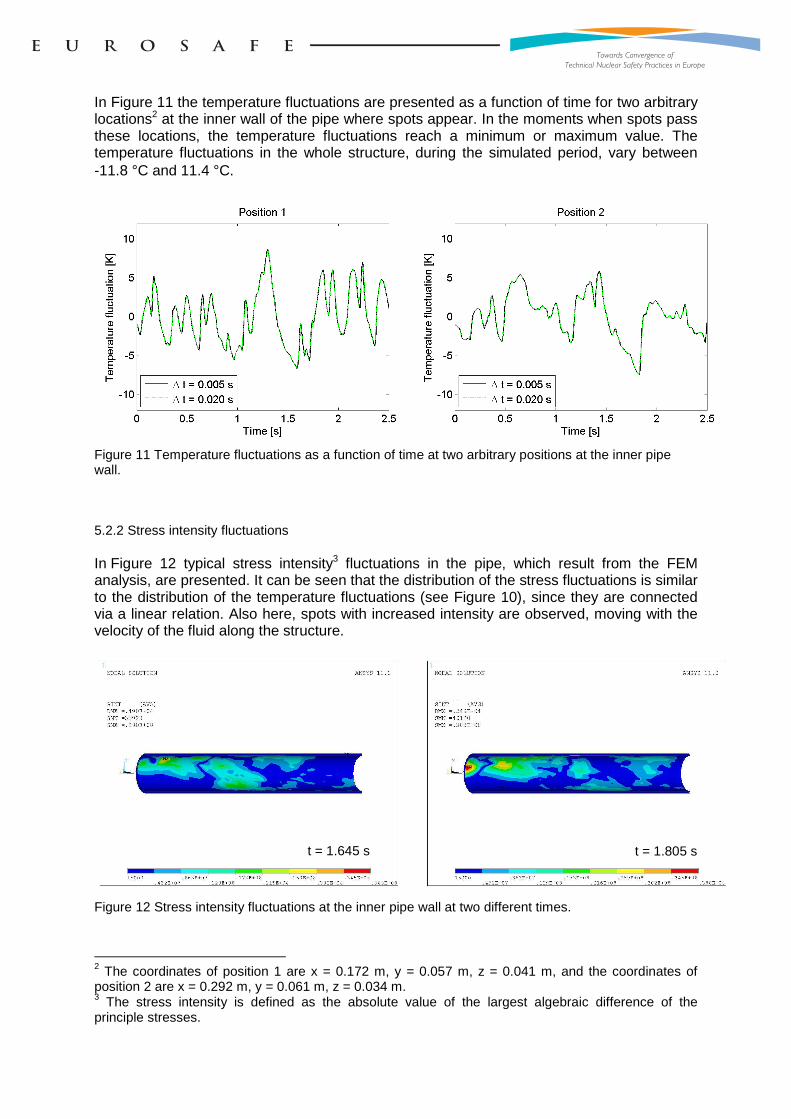
In Figure 11 the temperature fluctuations are presented as a function of time for two arbitrary locations2 at the inner wall of the pipe where spots appear. In the moments when spots pass these locations, the temperature fluctuations reach a minimum or maximum value. The temperature fluctuations in the whole structure, during the simulated period, vary between -11.8 °C and 11.4 °C.

Figure 11 Temperature fluctuations as a function of time at two arbitrary positions at the inner pipe wall.

5.2.2 Stress intensity fluctuations In Figure 12 typical stress intensity3 fluctuations in the pipe, which result from the FEM analysis, are presented. It can be seen that the distribution of the stress fluctuations is similar to the distribution of the temperature fluctuations (see Figure 10), since they are connected via a linear relation. Also here, spots with increased intensity are observed, moving with the velocity of the fluid along the structure.

Figure 12 Stress intensity fluctuations at the inner pipe wall at two different times.

2 The coordinates of position 1 are x = 0.172 m, y = 0.057 m, z = 0.041 m, and the coordinates of position 2 are x = 0.292 m, y = 0.061 m, z = 0.034 m. 3 The stress intensity is defined as the absolute value of the largest algebraic difference of the principle stresses.

t = 1.645 s t = 1.805 s

Figure 13 shows stress intensity fluctuations as a function of time for the same two locations as presented in Figure 11. For comparison, also the magnitude of the temperature fluctuations is plotted here. It can be seen that there is an approximate linear relation between the thermal loads and the stress response. The maximum stress intensity in the whole structure, during the simulated period, is 41.4 MPa.

Figure 13 Stress intensity fluctuations and temperature fluctuations as a function of time at two arbitrary positions at the inner pipe wall.

6 FATIGUE ASSESSMENT The demonstration case that is discussed in this paper was based on an experimental setup with a temperature difference of 15 °C between the hot flow and the cold flow [1]. The experimental setup was designed to validate the CFD model [8, 9]. However, the temperature difference of 15 °C is not sufficient to induce thermal fatigue. For the current simulations, the temperature difference between the hot flow and the cold flow was therefore increased up to 80 °C4. This leads to stress fluctuations in the pipe wall of maximum 41.4 MPa (see section 5.2). The design fatigue curve for austenitic steels, as given in ASME Boiler and Pressure Vessel Code [2], shows results for up to 1011 cycles. The minimum stress amplitude in the fatigue curve is considerably larger than the maximum stress amplitude in this demonstration case. This means that up to 1011 cycles, the temperature difference is still too small for thermal fatigue to occur. In the paragraph below, a more detailed description of the procedure to assess thermal fatigue is given. Starting point for the assessment are the stress fluctuations in the pipe, which are calculated as described in the previous section. As can be seen in Figure 13, these stress fluctuations, resulting from turbulent mixing, vary considerably in time, both in amplitude and frequency. To reduce such a complex signal to a set of cyclic loads, application of a cycle counting method is required. The most common method is the so-called rainflow counting method. Result of this procedure is a list of stress intensity amplitudes and the numbers of occurrence of the different cycles. Subsequently, the number of cycles during the simulated period is extrapolated to the number of cycles during the total lifetime of the component. The allowable number of cycles is determined using a design fatigue curve, as given by a design code. This

4 For the considered incompressible case, minimum and maximum temperatures are limited by the freezing and boiling temperatures of water. This imposes a physical limit at the temperature difference that can be applied.

is performed for each counted stress amplitude. Dividing the actual number of cycles ni by the allowable number of cycles Ni finally results in the so-called fatigue usage factor. By applying Miner's rule, the cumulative fatigue usage factor D is then determined as follows:

∑=

=k

i i

i

N

nD

1

where k is the number of counted stress amplitudes. According to ASME Boiler and Pressure Vessel Code [2], the loading of the structure is acceptable if the cumulative usage factor does not exceed 1.0. This requirement has to be satisfied for each point in the structure. To reduce computation time of the above-mentioned procedure, locations at the structure with stress amplitudes lower than the minimum stress amplitude in the design fatigue curves can be filtered out. As a next step, the developed strategy is planned to be applied to an actual plant case of crack initiation that has occurred at a nuclear power plant. Sufficient data for the (thermal) operating conditions and the time to crack initiation will however need to be available.

7 CONCLUSIONS By means of coupling CFD modelling, FEM modelling, and code assessment, a strategy was developed to assess thermal fatigue of complex mixing problems in nuclear power plants. In this paper, a description of this strategy along with its application to a specified test case was presented. For the CFD analysis, an experimentally validated CFD model was used. Coupling between the CFD model and the FEM model was established by a user written interface. It was demonstrated that temperature data is transferred properly between the two models. Based on the stresses calculated in FEM, fatigue assessment was performed according to ASME Boiler and Pressure Vessel Code [2]. Future work on this subject, based on the availability of experimental data, will be devoted to the application of the described procedure to situations where thermal fatigue has actually appeared or is expected to appear. Another planned activity is to compare the simulated CFD results with direct measurements of heat fluxes through the wall.

References

1. U. Andersson, J. Westin, and J. Eriksson. Thermal mixing in a T-junction. Technical Report U06-66, Vattenfall Research and Development AB, 2006.

2. ASME Boiler & Pressure Vessel Code; Section III Division 1 – Subsection NB; Class 1 Components; Rules for Construction of Nuclear Facility Components, 2007.

3. F. Blom, M. Church, and S. Willemsen. A simplified method to predict thermal fatigue in mixing tees of nuclear reactors. Fatigue Design Proceedings, Paris, France, 2007.

4. S. Chapuliot, C. Gourdin, T. Payen, J.P. Magnaud, and A. Monavon. Hydro-thermal-mechanical analysis of thermal fatigue in a mixing tee. Nuclear Engineering and Design, 235:575-596, 2005.

5. M. Dahlberg, K.-F. Nilsson, et al.. Development of a European procedure for assessment of high cycle thermal fatigue in light water reactors: final report of the NESC-thermal fatigue project. Technical Report EUR 22763 EN, Joint Research Centre, The Netherlands, 2007.

6. L.-W. Hu and M.S. Kazimi. LES benchmark study of high cycle temperature fluctuations caused by thermal striping in a mixing tee. International Journal of Heat and Fluid Flow, 27:54-64, 2006.

7. ITER, Material Properties Handbook, In-vessel Materials Database.

8. A.K. Kuczaj, B. de Jager, and E. Komen. An assessment of Large-Eddy Simulation for thermal fatigue prediction. ICAPP Proceedings, Anaheim, California, USA, 2008.

9. A.K. Kuczaj, and E.M.J. Komen. Large-Eddy Simulation study of turbulent mixing in a T-junction. XCFD4NRS Proceedings, Grenoble, France, 2008.

10. K.-J. Metzner and U. Wilke. European THERFAT project – Thermal fatigue evaluation of piping system "Tee"-connections. Nuclear Engineering and Design, 235: 473-484, 2005.

11. J. Westin, C. 't Mannetje, F. Alavyoon, P. Veber, L. Andersson, U. Andersson, J. Eriksson, M. Henriksson, and C. Andersson. High-cycle thermal fatigue in mixing tees. Large-eddy simulations compared to a new validation experiment. ICONE Proceedings, Orlando, Florida, USA, 2008.