AFWL-TR-86-06 AFWL-TR-86-06

A CONSTITUTIVE MODEL FOR SIMULATINGSOIL-CONCRETE INTERFACES

Zhen Chen

Howard L. Schreyer

'N New Mexico Engineering Research Institute

University of New MexicoAlbuquerque, New Mexico 87196

July 1986 EDTICE.LECTE

SEP1I

! Y Final Report

Approved for public release; distribution unlimited.

AIR FORCE WEAPONS LABORATORYAir Force Systems Command

LAJ Kirfland Air Force Base, NM 87117-6008

9 1-5

b6 9 16 05•-

AFWL-TR-86-06

This final report was prepared by the New Mexico Engineering ResearchInstitute, Albuquerque, New Mexico, under Contract F29601-84-C-0080, JobOrder 2302Y201 with the Air Force Weapons Laboratory, Kirtland Air Force Base,New Mexico. Dr. Timothy J. Ross (NTES) was the Laboratory Project Officer-in-Charge.

When Government drawings, specifications, or other data are used for anypurpose other than in connection with a definitely Government-related procure-,ment, the United States Government incurs no responsibility or any obligationwhatsoever. The fact that the Government may have formulated or in any waysupplied the said drawings, specifications, or other data, is not to beregarded by implication, or otherwise in any manner construed, as licensingthe holder, or any other person or corporation; or as conveying any rights orpermission to manufacture, use, or sell any patented invention that may inany way be related thereto.

This report has been authored by a contractor of the United StatesGovernment. Accordingly, the United States Government retains a nonexclusive,royalty-free license to publish or reproduce the material contained herein, orallow others to do so, for the United States Government purposes.

This report has been reviewed by the Public Affairs Office and isreleasable to the National Technical Information Service (NTIS). At NTIS, itwill be available to the general public, including foreign nations.

If your address has changed, if you wish to be removed from our mailinglist, or if your organization no longer employs the addressee, please notifyAFWL/NTES, Kirtland AFB, NM 87117 to help us maintain a current mailing list.

This technical report has been reviewed and is approved for pt:)lication.

Project 0 f~icer

/FOR THE COMMANDER

L I

DAVID H. ARTMAN, JR CARL L. DAVIDSONMajor, USAF Colonel, USAFChief, Applications Branch Chief, Civil Engineering Rsch Division

DO NOT RETURN COPIES OF THIS REPORT UNLESS CONTRACTUAL OBLIGATIONS OR NOTICEON A SPECIFIC DOCUMENT REQUIRES THAT IT BE RETURNED.

UNCLASSIFIEDSECURITY CLASSIFICATION OF THIS PAGE

Ia. AEPORT SE CURITY CLASSIFICATION lb, nRes'IiCTIVIE MAAKINGS

Uncl assified2& SECURITY CLASSIFICATION AUTHORITY 3. DISTRIBUTION/AVAILAaILITY OF REPORT

Approved for public release; distribution2b. OCLAISSIFICATIONiOOWNGRAOING SCHEDULE unlimited.

A. PERFORMING ORGANIZATION REPORT NUMSeRISI 5. MONITORING ORGANIZATION REPORT NUMBERIS)

NMERI WA8-9"(8.09) AFWL-TR-86-06

G&. NAME OF PERFORMING ORGANIZATION b. OFFICE SYMBOL 74. NAME OF MONITORING ORGANIZATION

New Mexico Engineering/ dDat tesibl.

Research Institute NMERI Air Force Weapons Laboratory5c. ADORESS (City. State and ZIP C4da) ?b. ADORESS WCity. State and ZIP Code)

University of New MexicoAlbuquerque, NM 87131 Kirtland Air Force Base, NM 87117

S.. NAME Of FUNOING/SPONSORING 8b. OFFICE SYMEO3L 9. PROCUREMENT INSTRUMENT IDENTIFICATION NUMBER

ORGANIZATION fit applicable)I F29601-84-C-0080

•c. ADDRESS (City. Statt and ZIP Code) 10. SOURCE OF FUNDING NOS.

PROGRAM I PROJECT TASK WCRK UNIELEMENT NO. NO. NO. NO.

62201F | 2302 Y2 0111. TITLE fInclude SecuityI C.•ueliedlion•n

A CONSTTTUTIVE MODEL FOR SIMULATING SOIL-CON R&TE TNTERFA(S . .12. PERSONAL AUTHOR(S)

Chen, Zhen; Schreyer, Howard L.13s, TYPE OP RIIEPORIT 13b. TIME COVEREO 14 AEO EOT(r.Mo.. Day) i IS.PG ON

Final Report IRoMNOV 84, TOkov 85 1986 July 7011. SUPPLEMENTARY NOTATION

17. COSATI CODES 18. SUBJECT TERMS lConlinue on reverse it necessry and identify by blocks number)

FIELD i GROUP SUB. R, Viscoplasticity, Concrete, Soils, Strain Rate, Strain0• 2 Softening, Interface, Localization, Strain Gradient

19. ABST RACT (Continue on iversr if n•geseary and identify by block numbert

This investigation explores the characteristics of deformation at the interface ofdissimilar materials such as concrete and soil. Based upon the basic features of thedeformation field, a new nonlocal approach for simulating soil-concrete interfaces isproposed. It is assumed that the stress field is a function of both strain and straingradients, and also, no relative slip occurs at the contact surface between soil andconcrete. By using computational plasticity and the finite element method, static anddynamic responses of the softer material next to an interface are evaluated numerically.Comparisons are made with other numerical data. Conclusions are given on the apparentsuitability of the approach.

2o. oISTRI8UTION/AVAILASILITY OF ABSTRACT 21. ABSTRACT SECURITY CLASSIFICATION

UNCLASSIFIED/UNLIMITED SAME AS PT OTIC USERS C Unclassified22s. NAME OF RESPONSIBLE INOIVIDUAL 22b. TELEPHONE NUMBER 22c. OFFICE SYMOLt.

I nclude A.,a Code)

Or. T. J. Ross (505) 844-9087 NTESAII

DD FORM 1473, 83 APR EDITION OF 1 JAN 73 IS ORSOLETE. UNCLASSIFIEDSECURITY CLASSIFICATION Or THIS P

CONTENTS

Sect i onP

I INTRODUCTION 1

II SCOPE OF THE INVESTIGATION 3Objective 3

Interface Phenomena 3

Present Status of Models for Interfaces 6

Procedure 9

III MATHEMATICAL MODEL 10

Assumptions 10

Basic Equations 11

A Constitutive Relation for the Interface Under Shear 18Features of the Model 18

IV COMPARISONS WITH OTHER. NUMERICS'. DATA 25

Dynamic Response of the Interface Under Shear 25

Static Response of the Interface Under Shear 45

V CONCLUSIONS 57

REFERENCES 58

LIST OF SYMBOLS 60

Accesion For

NTIS CRA&IDTIC TAB L1U:;arnouriced E5

By_ ...............................................

Di A. ib:; tior: I

Availability Codes

' Avoil a' d /orDizt 6 p•. cidl

fr-

,.-ý X rIL (W-M r %f~'~~NU~ r W_-Vn LF' WWV~ R U Wl 'lj ~v w uVV1.1 V wvN-. ~)~f ~T f v~ W%%.v~ 4t 'V~ r V 1MAV

ILLUSTRATIONS

SPage

1 Geometry for the interface problem 4

2 Effect of the parameter n in the hardening regime 19

3 Effect of the parameter as in the softening regime 20

4 Effect of mean pressure on the stress-strain curve 21

5 Effect of the parameter a3 , or the invariant of straingradient, on stress-strain response 22

6 illustrations of loading, unloading, and reloading in

the hardening and softening regimes 24

7 Finite element mesh of the soil bar and the shapefunction used 27

8 Illustration of elastic stress wave at various times 33

9 Spatial distribution of stress at various times 34

10 Spatial distribution of stress at various times usingthe current approach 35

11 Spatial distributions of displacement field at varioustimes 36

12 Spatial distribution of displacement field at varioustimes using the current approach 37

13 Spatial distribution of strain at various times 38

14 Spatial distribution of strain at various times usingthe current approach 39

15 Shear stress-strain path for element 1 at time t = 1.7 40

16 Shear stress-strain path for element 20 at time t = 1.7 41

17 Distribution of displacement at t = 1.7 for differentmeshes 42

18 Distribution of stress at t = 1.7 for different meshes 43

19 Distribution of strain at t = 1.7 for different meshes 44

20 Strain distribution for static response in elasticregime 47

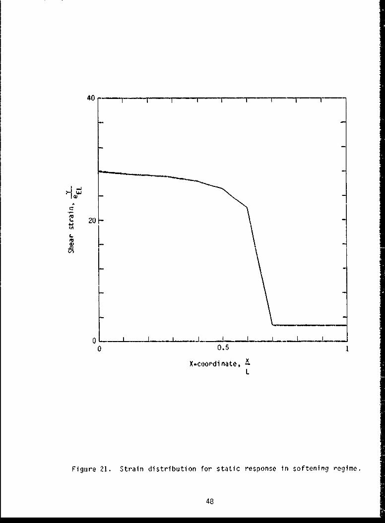
21 Strain distribution for static response in softeningregime 48

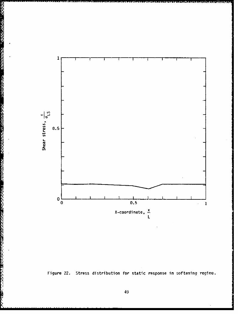
22 Stress distribution for static response in softeningregime 49

23 Shear stress-strain response of element 1 50

iv

ILLUSTRATIONS (Concluded)

Figure Page

24 Shear stress-strain response of element 6 51

25 Shear stress-strain response of element 10 52

26 Strain distribution for different meshes to showconvergence 53

27 Effect of the parameter a3 , or the invariant of straingradient, on the static response near the surface 54

28 Shear stress versus the displacement of the end of thesoil bar for various values of mean pressure 56

V/vi

I. INTRODUCTION

Because of failures in structures caused by ground motion from earth-

quakes or explosives, soil-concrete interaction problems are playing an

increasingly important part in engineering design procedures and safety analy-

ses. The information available, however, is still sparse due to the complex-

Ity of the nonlinear response of these geologic materials.

In the past, many models for representing interfaces were based on

Coulomb's law, i.e., no slip between two bodies will occur unless a critical

tangential stress is reached, and the relative motion is constrained to be

along the contact surface if the critical state is reached. For dissimilar

materials like concrete and soil, however, Coulomb's law may not be appli-

cable, since slip does not occur at the interface. Instead of slip, a band

with large shear deformation is observed in the weaker of the two materials,

and these observed zones with large strain gradients cannot be automatically

predicted. Nevertheless, the simple friction approach has been utilized with

either slip lines or special interface elements to obtain computational pro-

cedures, which in turn introduce questions oi st1bility and coiputational

complexity.

This research addresses a new approach for simulating a soil-concrete

interface where both theoretical and computational aspects are kept in mind.

The idea relies on the observations that (1) slip does not occur for the soil-

concrete interface until a failure state is reached, and that (2) progressive,

distributed damage produces a band of permanent deformation in the soil adja-

cent to the interface. The lateral dimension of the band appears to depend on

the physical characteristics of the materials. The only way to predict a

finite zone of localized deformation under a homogeneous state of stress is to

utilize a nonlocal constitutive law. Furthermore, it appears that localiza-

tion occurs only when softening is present. Thus, if a nonlocal constitutive

model is postulated where softening is governed by both strain and the gradi-

ent of strain, then softening localizes into a finite region, which cannot be

predicted by using a local constitutive model. With the use of a nonlocal

constitutive model for soil, and the assumption that the interface initiates

softening in the weaker of the two ,aterials, the deformation field adjacent

to the interface can be simulated.

NI 10Q- IV V1 Ti =A r n v VVV I vNM%_VeI

In this study, numerical solutions of a model problem with dynamic and

static shear loadings are compared with other numerical data.- ýt was conclude

that the new approach is reasonable in in engineering sense, and it is feasi-

ble to incorporate the model into existing finite element and finite differ-

ence computer codes.

2

II. SCOPE OF THE INVESTIGATION

OBJECTIVE

Based on existing experimental data, the general behavior of soil adja-

cent to a concrete interface can be described. Some assumptions are proposed

to construct a new nonlocal constitutive model for simulating the behavior of

soil in the vicinity of an interface. Using computational plasticity theory,

the characteristics of the model are discussed. Existing theoretical data

are used for comparison with the model. Conclusions and comments on possible

future research are given.

INTERFACE PHENOMENA

Interface behavior has drawn considerable attention in recent years,

especially for the following engineering problems: retaining wall design,

skirt friction in piles, soil-structure interaction for nuclear power plants

subjected to earthquake loadings, and for underground structures subjected to

blast and ground shock.

Due to the limitations of experimental techniques, and the assumptions

that Coulomb's friction principle holds for interfaces of deformable bodies,

there have been a limited number of investigations of interface phenomena.

Existing experimental data do not provide an accurate view of the deformation

field in the vicinity of the interface. Nevertheless, an approximate descrip-

tion and some knowledge of the soil-concrete interface can be obtained by

carefully analyzing the data. This research discusses the problem from a

continuum point of view and presents an alternate viewpoint based on the

observation that, adjacent to an interface, a region with a large gradient of

strain is often formed for shear loading (Fig. 1). An important part of this

work was to develop a procedure for describing this phenomenon.

Among the investigators dealing with soil-concrete interface phenomena,

Huck, et al., (Refs. I and 2), were unique in that both experimental and ana-

lytical investigations were performed. Also, several valuable references were

given. From their interface tests under static arid dynamic shear loadings, it

was concluded that interface shear" resistance is strongly influenced by the

3

u (Displacement)

I x

Concrete SoilP

(Mean pressure)

Shear strain

Sx

Figure 1. Geometry for the interface problem.

4.

soil type, the stress normal to the interface, and the relative size of tile

interface roughness with respect to the soil grain diameter. Total interface

shear resistance is reduced below the soil shear strength due to softening of

the expansive soil and loss of adhesion. It appears that localization of

large deformations usually occurs adjacent to the interface, in a region char-

acterized as a shear band, which increases gradually in thickness with coritin-

ued increase in applied static displacement. After each interface test, the

final dimension of the band of permanent deformation is not the same for

different materials.

Drumm and Desai (Ref. 3) worked on soil-structure interface tests under

static and cycliP loadings by using a new testing apparatus called thle "Cyclic

Multi-Degree-of-Freedom" device. They indicated that the behavior of a struc-

ture resting on, or embedded in a foundation depends on the material proper-

ties of both the structure and the foundation medium, and on the types of

applied loadings. Soil-structure interaction becomes more significant when

structures are subjected to dynamic loadings. The interface strength was

found to be less than that of soil, and gradual separation may occur at or

near the interface.

Vermeer (Ref. 4) investigated interface behavior between granular materi-

als and metals during powder compaction in a die. There are two friction

angles in powder compaction: one for powder-wall friction, and another for

powder-powder friction. These two angles were shown to be related for compac-

tion in a die with rough walls. From tests, it was pointed out that the

powder-wall slip plane is in fact a thin shear band.

A number of factors, not directly pertinent to the basic soil-concrete

interface problem, might act to obscure the true phenomena. However, by ana-

lyzing the experimental apparatus and test results mentioned above, it was

possible to draw the following descriptions for tile mechanism of an interface

consisting of'concrete and particulate material.

Imperfections at or near the soil-concrete interface will initiate pro-

gressive distributed damage such as dispersed inicrocracking, void formation,

or loss of interparticle contacts. From the macroscopic viewpoint, large

deformations can be observed adjacent to the interface, and the size of

I.

the band of permanent deformation will enlarge with increase in thle applied

displacement. Althlough relative motion occurs between particles as soon as

external loading is applied, no slip seems to occur as the stress is

increased. If deformation continues to Increase, the stress will reach a peak

and then decrease in what is called the postpeak regime. Slip appears to beinitiated somewhere in the postpeak regime. When macroscopic slip occurs, the

dimension of the band seems fixed and the total deformation field is not con-

tinuous. Thus, slip might be considered as a mechanism that occurs after the

Av formation of the shear band.

PRESENT STATUS OF MODELS FOR INTERFACES

During the past 20 years, evaluation of the dynamic interaction between

a structure and the surrounding medium has been accomplished by two

approaches, consisting of either the use of classical continuum mechanics, or

the finite element method.

The first approach simulates the effects of soil on the structural

response by a series of springs and dashpots representing a theoretical half

space surrounding the structure. This method is generally limited to elastic

or viscoelastic representations of soils. The finite element method is an

alternative approach to solving problems in continuum mechanics. Althoughbased on the same principles of mechanics, it changes the partial differential

equations governing the motion of the continuum into a finite set of ordinarydifferential equations in the time domain which makes it possible to incorpo-

rate a more reasonable constitutive relation into the interface model. A

survey of both the spring-dashpot and finite element approaches to thestructure-soil interaction problem was given by HadJi-n, et al., (Ref. 5).Also, Seed, et al., (Ref. 6), presented an evaluation of the strengths and

v~.weaknesses of the two approaches. Although the above information reviewedonly the efforts in an infant period of research, the history of development

in this field was quite helpful.

Recently, emphasis in researchi nas been on improviny the description ofinterface behavior, not only in the prepeak rejime. but also in the postpeak

regime, while computer-based techniques have supplied powerful tools for

analyses. Mathematical models are set up witn the use of both conservation

6

principles and constitutive relations. Conservation principles, based upon

classical physics, or Newtonian physics, have been well established. Hence,

accurate descriptions of the behavior of materials have become more and mora

important. Desai and Siriwardane (Ref. 7) reviewed and explored the constitu-

tive behaviors of engineering materials, with emphasis on geologqcal materials

such as soil and concrete. Currently, in addition to the classical continuum

appruach for soil-concrete interface, both the particle approach, together

with statistical analysis, and the nonlocal continuum approach have been

proposed.

Huck, et al., (Refs. 1 and 2), derived a soil-cv,,crete interface model

using basic frictional mechanisms as applied to a particulate soil. The par-

ticle approach employed the mechanisms of adhesion, plowing, and lifting. The

concrete interface surface was considered as a flat plane, with protruding

spherical caps representing the roughness or asperities of the concrete sur-

face. Soil in contact with the concrete interface was modeled as spherical

particles of known size, but randomly distributed over the interface surface.

In the model, relative slip between soil and concrete occurred if, and only

if, a critical tangential stress was reached, and the relative motion was

assumed to be along the contact sdrface. The tangential stress was propor-

tional to the normal stress. It appears that gradual formation of a shear

band could not be predicted. This constitutive model is, by nature, a classi-

cal Mohr-Coulomb model.

Vermeer (Ref. 4) investigated interface response in powder :ompaction by

means of a nonassociated perfect-plasticity model. The idea of sliding on a

single plane was considered much too restrictive. Therefore, a new idea

allowed small slipping motions on an infinite number of closely spaced paral-

lel surfaces, and used the Mohr-Coulomb criterion. To calculate the stress

and density distributions at several stages of the loading process, three

approaches were suggested. The first was the use of a nonassociated consti-

tutive model and a fine mesh near the walls of the die, so that a thin shear

band could develop. The second consisted of special thin interface elements

to model the shear band along the wall. Frictional sliding was implemented

directly as a mixed boundary condition in the third approach.

7- - - - - - - - -- - - -m

Drumm and Desai (Ref. 3), and Oden and Pires (Ref. 8), describe the con-

stitutive behavior of the interface by using frictional principles with some

modifications. Either elasticity or perfectly-plastic relations have beenused for simulating soil-concrete interface by these authors as wel I as

others.

From the research efforts mentioned above, it was found that assumptions

based upon frictional theories were commonly adopted, and numerical methods

are under active development to solve the continuum models. It is doubtful,

however, that frictional theories are useful for representing interfaces

involving materials with disparate properites such as concrete and soil. In

addition, there are some unpleasant features associated with numerical proce-

dures for frictional models, such as size-dependent response and 1.omputational

difficulties due to special algorithms. To obtain a basic understanding of

the inherent physical nature of the interface, and to apply the knowledge to

engineering practice, the exploration of a more reasonable and convenient

approach seems necessary.

With the development of knowledge for heterogeneous materials, a nonlocal

continuum theory offers hope for modeling the postpeak behavior of geological

materiais. The word "nonlocal" in this context means that stress depends both

on strain and strain distribution. The latter can be given tirough the use of

integrals and a weighting function, or by derivatives of strain. The full

force-deformation behavior, but not necessarily the stress-strain relation-

ship, beyond peak stress has been documented for concrete, rock, soils, and

sore other- materials under uniaxial stress. One approach was to model the

postpeak behavior by using plasticity and the reduction of stress with strain.

However, serious theoretical and computational ditficulties caused by strain

softening have occurred, and they have been intensely debated at recent con-ferences. Valanis (Ref. 9), Sandler and Wright (Ref. 10), and Read and

Hegemier (Ref. 11) discussed in detail the various arguments concerning strain

softening. Bazant, et al., (Ref. 12), incorporated strain softening into a

consitutive model by using a nonlocal continuum theory. Schreyer and Chen

(Ref. 13) investigated the effects of strain softening and lucalization in a

structure by assuming that stress was a function of both strain and strain

gradients. it was concluded that current experimental techniques could not

rule out strain softening because instrume tation has not been designed toidentify localization and to measure strains in the resulting small zones.

8

Also, several types of nonlocal approaches have overcome obstacles caused by

strain softening. At present, (1) a finite strain-softening zone, (2) nonzero

energy dissipation, and (3) numerical stability of dynamic problems have been

achieved. Additional research is required to generalize the theory on strain

softening. Incorporating strain softening into constitutive models would be

useful and feasible in engineering practice if the response of a material can

be predicted.

Considering the interface phenomena, it has been suggested that a one-

dimensional model (Ref. 13) be used to simulate the weaker of two materials at

an interface, with the assumption that an interface, in effect, weakens the

softer material. If an interface can be dealt with in such a manner, then

special algorithms would not be necessary to handle interfaces, and further-

more, a band of permanent deformation adjacent to the interface will be pre-

dicted which is representative of physical behavior. Using conventional,

constitutive-equation algorithms and finite-element methods, static and

dynamic response featLes of the interface can be obtained with a simple,

convenient calculation.

Since an ultimate objective i" 'o have a completely general model, this

research provides a three-dimen al formulation. However, applications are

limited to the one-dimensional

PROCEDURE

Several assumptic )osed based upon existing experimental data.

A three-dimensionai of1stitutive model is then developed for simu-

lating the soil-concrete interface by the use of nonlinear plasticity theory.

The model reflects the characteristics of geological materials more accurately

than a bilinear constitutive model. Features of the model are explored under

different values of mean pressure and strain gradient. In order to verify the

model for an interface under dynamic shear loading, the finite element method

is used, together with explicit time integration and comput tional plasticity

techniques, to obtain numerical solutions which are compared with existing

theoreticai data for the wave propagation problem. The conclusion of this

research shows results for static she. oading.

9

III. MATHEMATICAL MODEL

ASSUMPTIONS

Making assumptions was the first nontrivial step in the formulation of

the new model. Reasonable assumptions yield good results with a modest

effort, whereas poor assumptions can lead to considerable computational

effort. Making good assumptions depends on engineering experience and intui-

tion. Furthermore, each assumption has its own limitation which must corre-

spond to the problems being considered.

As mentioned previously, there is not enough experimental data to provide

a good qualitative description of the behavior at soil-concrete interfaces.

For example, it is still uncertain at what stage of the loading path the mac-

roscopic slip between concrete and soil occurs, if it occurs at all. The

following assumptions were made to construct a new nonlocal continuum model

which is different from the usual Mohr-Coulomb model.

Assumption 1--Slip does not occur at the contact surface between concrete

and soil under shear loading. Instead, with an increase in load, a shear band

will form due to dispersed microcracking. This shear band represents a local-

ization of deformation that is accompanied by softening.

Assumption 2--The imperfection of the soil-concrete interface reduces the

strength of the soil, so that with large enough loads, the softening is initi-

ated in the region of soil adjacent to the interface. With this assumption,

the roughness of the concrete surface is simulated through the strength prop-

erty of the adjacent material, rather than through a friction coefficient.

The result is that softening is initiated at a lower load for a smooth inter-

face compared to a rough interface, but the evolution of softening and the

localization zone will be governed by the constitutive equation.

Assumption 3--A nonlocal constitutive theory is required to represent the

localized behavior of softening in soil. This theory provides a means for

controlling the size of the localization.

Assumption 4--A suitable nonlocal theory is obtained if the limit stress

depends on the strain gradient. Read and [Iegemier (Ref. 11) indicated that

10

strain softening is not a true material property, but is simply a manifesta-

tion of the effects of progressively increasing inhomogeneity of deformation.

However, an alternate interpretation, that equally explains the observed phe-

nomena, is that softening occurs only in the presence of strain gradients.

The assumption that limit stress reduces with the strain gradient is therefore

a simple mathematical representation of the observation.

BASIC EQUATIONS

To simulate the general constitutive behavior of soil-concrete inter-

faces, a nonassociated Prager-Drucker model, with some modifications, was

adopted to provide appropriate inelastic response features of soils. Such a

model does not accurately reflect the behavior of soils, but it is one of the

simplest inelastic models that can be used. If strain gradients are incorpo-rated into a complex model, it becomes difficult to separate and study the

various features individually.

In the theory of plasticity (Ref. 14), the case of combined stresses is

represented by means of the concept of a yield surface. For any point in a

material region, assume that there exists a domain in the stress space inwhich material behavior is governed by elasticity theory. The hypersurface

bounding this domain is known as the yield surface. If the material is per-fectly plastic, the yield surface does not move. If the yield surface expandsout to a limit state, the material is said to harden, while the material

starts to soften as soon as the yield surface contracts in a controlled man-

ner. The motion of the surface is governed by internal variables which recordthat part of the stress history involving inelastic behavior and other varia-

bles directly affecting yield. The motion of the stress point inside the

surface, i.e., in the elastic domain, is not dependent on internal variables.

In the general constitutive model used in this research, the internal vari-ables considered included an inelastic strain invariant e , the mean pressure

p . .- iP, and a strain gradient invariant g . The indicial notation was preferred,because this notation allowed us to write equations in a much shorter form

than would otherwise be possible. In representations of first and second

order tensors, subscripts refer to the indicial notation, while superscripts

imply the definitions of tensors, e.g., the elastic or inelastic part of the

strain tensor.

In the following part of this subsection, the modified Prager-Drucker

yield-surface function is discussed first; then the potential function and

some important formulae are given. To solve the nonlinear constitutive equa-tion, an incremental numerical procedure is described based upon computational

plasticity theory.

For convenience in numerical calculations, the yield surface is defined

in a dimensionless form as:

0- ( + a 1P) Gr HF 0 (1)

0LS

in which aLS is the limit value of the shear stress-shear strain curve, and od

is the second invariant of deviatoric stress air as follows:

d 1/2(22 = ij ji (2)

d (3)•'ij O ij -; 3kk ij 3

The function H incorporates both strain hardening and softening according to

the following relations:

H = L + (L - Lo) sin i. o(< e <e (4)

-i -ie -eL

_.i "a61 -a,

H (Lp- a ) + a5 -L e + a4 >eL (5)-iIeL /

The total strain tensor is divided into an elastic part and an inelastic part,

as follows:

e ieij e eij + eil (6)

12

Then, one of the internal variables in Eqs. 4 and 5, the inelastic strain

invariant is:

i d( ' di di) 1/2ei : J deij eli (7)

where

di (8)e i j aeij - 3 ekk 6ij (8)

The values of H at initial yield and the limit state are denoted by L0 and Lp

respectively. The value of i at trhe limit state, eL', is assumed to be inde

pendent of path. The parameter n controls the shape of the stress-strain

relation in the hardening regime while as controls the shape during softening.

The softening formulation for H given in Eq. 5 provides a horizontal slope at-i

the limit state and a limiting value for H of a4 for large e

The invariant (ji) of the strain gradient is defined by the relation:

i (e', e ) n /2 (9)= ki, kn,n /

The strain-gradient factor, G r' in Eq. I is assumed to ýe of the form

-iGr (1 - a )e~a3g + a2 (10)

where the parameter a3 controls the rate at which Gr decreases with g . For

i equal to zero, Gr is unity, and for large gi, the function Gr asymptot-

ically approaches a 2 .

To be consistent with experimental data (Refs. 1, 3, and 7) for

geological and other frictional materials, the mean pressure

p .I (11)

3

was also incorporated into the constitutive model as a coefficient of the

parameter al-

13

With the use of a nonassociated flow rule, the inelastic part of the

strain tensor is given by

i __________

de i dx - (12)dij 30dl S@ij

where the potential function was chosen to be

H (13)°LS

so that the inelastic strain tensor contains no volumetric component. This is

consistent with metal plasticity but is not entirely appropriate for soils

which display inelastic volumetric strain. The inclusion of inelastic volu-

metric strain would have provided a complication that has no direct relation-

ship to softening and localization.

The elastic part of the strain tensor is related to the stress tensor

through the elastic constitutive equation:

Oij =ijkl kl (14)

where the tensor Cijkl is normally restricted to the isotropic case.

Now the general constitutive model is established. This model is linear

in the elastic regime, and nonlinear in the hardening and softening regimes.

Mean pressure increases the strength of the material, while strain gradient

reduces its strength.

In the numerical procedure, an incremental scheme was adopted to solve

the nonlinear constitutive model. The incremental relations are summarized

below:

e i&e = Ae + 4ei (15)

eAoij = C ijkl Aekl (16)

14

Ae1 =AX- (17)iij

-ii /2 ' Ae" 1i/2 (8

In practice, the total strain increment aeij, the total strain from theprevious step (eij)p, and the stress from the previous step ( ij)p are known.

The difficult problem is that the elastic and inelastic part of Aeij are iunknown. To solve the above ,onlinear equations with unknowns eij, ,ij eijV

Ax, and aeij, an iterative procedure was used. The basic ideas are those of

computational plasticity (Ref. 14). The following is an outline of the con-

stitutive equation algorithm.

Step 1--The user inputs components of the total strain increment tensor,

material parameters, and other control parameters. Existing values of stress,

total strain, elastic strain a.Ad inelastic strain tensors are stored as

(aij)p, (eij)p, (eej)p and (e.i )p, respectively.

Step 2--Fi.st, assume that the step is elastic:

eAeij = aeij

SteL3--For future use, calculate:

d

ij ai 2 0 LS0

F ' . . . C ij k l -__

aA ij 0kl

I = 0 (I = iteration count)

15

Step 4--Find increments in stress components:

AU = Cj kl ael

ii jkl ki

Step 5--Update old stress components and the iteration count:

lJ" (IIj )p P+A0ij

a i, + Ig.

jSte6--Evaluate ; and the yield function F.

Step 7--Check the yield function F:

(a) If F < 0 and I = I (i.e., the first step), then the solution is

elastic and the stresses are correct. Go to Step 12.

Otherwise,

(b) If IF! < e and I > 1, then the plasticity solution has been obtained

and the stresses are correct. Go to Step 12.

Otherwise, go to Step 8.

Step_8--The iteration begins. The following procedure is used to solve

for Ax:

For the first step, (I = 1):

(F),= - (one-step Newton-Raphson procedure)

(F'),

For other steps (I > 1):

(FP) 1 = (___" (F)I-I (backward finite difference)

(F)1 (A•x) 1 (F)1(AX). - =-_ _ _ _ _ _

(F')I (F)11 - (F)1

16

U

Step 9--Update inelastic strain increments:

(Alj)l o (iieijl-i 4. (alx), Tij

Step 10--Recalculate elastic strain increments:

(AG e (Ae e (Ax) T

(ejI = e I- I ij

Step 11--Go to Step 4.

Sep -- Update inelastic strain tensor:

i , i ieii k •ei p ij

Step 13--Compute inelastic strain invariants:

Ai (2 di Aedi\ /2

p +

S.tep 14--Update elastic strain and total strain tensors:

e e = e

e! i = (elj)p + Aeij

i eAeij = Aeij + Ae

-

eij = (eij)p + Aej

Step 15--Exit for next increments of total strain tensor components.

In the algorithm described above, the accuracy and number of iterations

are controlled through the magnitudes of the convergence parameter e and the

increments of total strain. Small values of e require generally more itera-

tions and, hence, more computer time. This algorithm is simple and appears to

be effective in an engineering sense.

17

A CONSTITUTIVE RELATION FOR THE INTERFACE UNDER SHEAR

The constitutive model needs only to be one-dimensional for the soil-

concrete interface under shear loading as shown in Fig. 1, and can be derived

directly from the above general equations. The stress state of the problem

is:

011 = 0 2 2 Q 033 ! 023 ' 013 = 0 (19)

The use of Eq. 19 results in the relations:

E e (20)2(1+v)

e i2 e + e (21)e 1 =e2 +1e2

F -T3- 12 - H(I+aP) (1-a 2)ea3§g +a2F 0 (22)aLS

de 1 2 : d a, - (23)

To simulate the behavior of soil-concrete interfaces, Eqs. 20-23 are used

to represent the constitutive characteristics of soil, and the interface is

assumed to initiate failure. The following subsection illustrates the effects

of mean pressure and strain gradients on the model through the use of tile

constitutive equation subroutine. The results should be helpful for

understanding the global behavior of a soil-concrete interface.

FEATURES OF THE MODEL

A total of eight parameters in Eq. 22 can be used to simulate different

types of materials. Among these parameters, Lo and Lp are ths elastic limit

and tVe peak value of the shear stress-strain curve respectively, while a2 and

a, are chosen so stress will not be null in the postpeak regime, a reasonable

assumption based on experimental observations. Parameters a,, a , a,, and n,

control the basic shape of the stress-strain curve. For the purpose of

illustration, the effects of these four parameters are shown separately in

Figures 2, 3, 4, and 5 in which stress has been normalized with respect to the

18

- n

1.0

4V)

0.5

SI 1 ! OI I 1 1 __ 1 -- 1 .1 1 1 1 -! _- --I I I _

04 8

SShear strain, e1e eEL

° Figure 2. Effect of the parameter n in thle hardening regime.

1409

1 ., 5 -- 'I "I-t • -I -I- i I I I I•-- • • -t '• 'r '•...f

S. .. . as a ,2

v•a5 51

-- a$ - 0.5

-- -a 5 - 0.25

1.0-

0~~ - I

0 48e,2

Shear strain, -_-e EL

Figure 3. Effect of the parameter as in th~e softening regime.

20

1.0

, .- - -I

0.0 I

I K.

4--

VIV

aP =0a P =0.2alP =0.4

0 4 I0

4

e12Shear strain, -

eEL

Figure 4. Effect of mean pressure on the stress-strain curve.

21

1.5 -- T-r--rT-r--i--- I -- TT-T

Sa3 - 0.02. .. a3 0.04

1.0

bc*

S0! .- . ,. "-

V.

Shear strain, _e EL

Figure 5. Effect of the parameter aa, or the invariant of straingradient, on stress-strain response.

22

stress at the limit state, 1LS' and strain has been normalized with respect tothe strain at the elastic limit, eEL. The other material and control parame-

ters used in the numerical investigations were assigned the values:

Lo = 50 /3 Lp = I00 3 a 2 = 0.1 aLS = 1 g 10

a4 =10/3 -=2 e 10 e E 25 P =1002(1+v) eEL

e = 10-4 LS = 100 / _3 Ae, 2 =0.5

Figure 2 shows the effect of the parameter n in the hardening regime for

a, z 0, a, = 0, and a. = 1. Note that the curve is smoother with a smaller

value for n.

Figure 3 shows the effect of the parameter a5 in the softening regimefor a, = 0, a, = 0, and n = 0.5. By changing the values of a., differentpostpeak behaviors can be simulated. As a limiting case, the material is

perfectly plastic when a. is equal to zero.

Figure 4 illustrates the effect of mean pressure on the stress-strain

curve for a 3 = 0, a. = 0.5, and n = 0.5. As shown in the figure, the strength

of the material increases with an increase in mean pressure.

The effect of the strain gradient on the stress-strain curve is shown in

Figure 5 for a, = 0, a. = 0.5 and n = 0.5. One of the assumptions used in thecurrent model is displayed in this figure, i.e., the stress is a function of

both strain and strain gradient. The strength of the material is reduced withan increase in strain gradient.

To conclude this section, Figure 6 shows the loading, unloading, and

reloading of the model by changing the sign of Ael 2 for a, = 0, a 3 = 0,

a5 = 0.5 and n = 0.5.

The above figures show that the current model can represent many response

features that are typical for geological materials (Refs. 1, 3, and 7). Iflarger values of Ae1 2 are used, the response becomes less smooth, but theessential features are retained.

23

1.5

Loading

1.0

Unloading /-

0.

4 8

eShear strain, _EL

Figure 6. Illustrations of loading, unloading, and reloading in thehardening and softening regimes.

24

IV. COMPARISONS WITH OTHER NUMERICAL DATA

DYNAMIC RESPONSE OF THE INTERFACE UNDER SHEAR

The constitutive relation for a material point in soil has been estab-

lished. In order to obtain the global response of the soil-concrete interface

under dynamic shear loading, the finite element method (Ref. 15) together with

a time integrator (Ref. 16) can be used. These two discretization processes

provide approxinnate solutions of complex problems for which analytical solu-

tions might not be available.

In this section, finite element approximations over a given geometrical

domain are described first. Then, the field variable is discretized in the

time domain by using a Newmark integrator in time.

For the soil-concrete interface shown in Figure 1, the notations of engi-

neering shear stress (t) and strain (y) are used for convenience. It is

assumed that ' = 1 2 , and that the displacement (u) is a function of (x) only,and in a unique direction, perpendicular to (x).

With these assumptions, it follows that

y = u, (24)

and the one-dimensional wave equation for shear is given as

=,x putt (25)

where p is the mass density.

In the elastic regime, stress *is related to the displacement through the

relation:

E= y - - u, (26)

2(1 + v)

Plasticity theory is used to determine stress in the hardening and softening

regimes.

25

~ ~ *4~- .4 ., j* 4 -

For the soil bar of length (L), the variational formulation of Eq. 25 is

Lf(r' - p u'tt) w dx = 0 for all w (27)0

where w Is the test or weighting function. After performing an integration by

parts, it follows that

L L fL ff w,x T dx + f p w u,tt dx -w + w 0 for all w (28)

A Ao 0

where fL and f are the external loads applied on the ends of the soil bar,

x = L, and x = 0, respectively.

Divide the soil bar into elements of equal length (h) as shown in Fig-

ure 7 and use linear element shape functions *i' i.e.,

1 - n (29)

nP n (30)2

where

X - X.

n - (31)h

Then the integrals in Eq. 28 can be converted to a sum with the result that

'e dn + f w, T+ -fo ut en wL oýwe= 1

e

for all w, where N is the number of elements and p is the element mass den-

sity. The global functions u, tt, w, W, and w,x are computed element by

element in the domain of the problem 0 < x < L. In an arbitrary element (e),

these functions are interpolated as follows:

26

Interface fL (t)

< ~P-

, xo x, x.z xI xt+1 x n

2 •.-n

xx

>i e 2

Figure 7. Finite element mesh of the soil bar and the shapefunction used.

27 -

e e1 + e2u'tt O utt * 1I u'tt 402 (33)

Ire =el ýj+ Ce2 2(4

we = wel t + we2 *2 (35)

we el ee 1 n + we2 *, (36)

where the superscript el denotes the left node of each element, and e2, theright node.

If the consistent element mass matrix is defined to be

e eMij = p h f ýi ýj dn (37)

and the element internal Force vector is

.Ie X er. n i dii (38)0 ,r

then, an alternate form of Eq. 32 is

wei e Iej + le -fWL f (39)I w MiJ u'tt + E fi we - WL + 2 o w39

= J=1 i1 A A

for all w.

Now relate the global nodal values, Wk" Uk tt, and the element nodal orei eilocal values, w , U'tt, as follows:

Wk = w(k-)2= w k1 (40)

tk,tt = (i)? - tk (41)

where the subscript k refers to the node number, and the two superscriptsdenote the element number and the element node number, respectively. Assume pis constant for each element. Then, with Mij representing the global mass

28

% . 1%.ý -VW 1! 1 - ' n ýA -

matrix and fiP the global force vector, the variational formulation of the

equation of motion can be written in indicial notation as

Mij uj tt = fi (42)

whe re

1/3 1/6 0. 0 ._1/6 1/3 1/6 0 . 0

M ]ph0 1 /60 0. 0 (43)• j 0 0 0

o .. 1/3

and

fo0

A + +A

fi •(T22 + 31) (44)

f2

A +A

Equation 42 represents a set of ordinary differential equations defined

in the time domain. The global force vector is the sum of the externtl force

and internal force vectors, through which the constitutive equation sub-rou-

tine is used. To solve this set of equations, a time integrator is used. To

make the system explicit in time, a diagonal mass matrix is required. The

diagonal mass matrix is constructed by summing each row of the global mass

matrix as shown in Eq. 43, and putting the sum of each row into the corre-

sponding diagonal position. Although the time step must be chosen according

to the stability condition, no matrix storage is required, and calculations

using the explicit method are much simpler than those using the implicit

method.

Introduce the discrete values of time,

t = ns for a fixed time step s (45)

29

le nwhere the superscript n is an integer denoting the discrete time, and let ui,n nnv., and a. be approximations to displacement ui(tn), velocity vi(t , and1' 111

acceleration ui tt(tn) at node i respectively, A particular form of the

Newmark integrator is

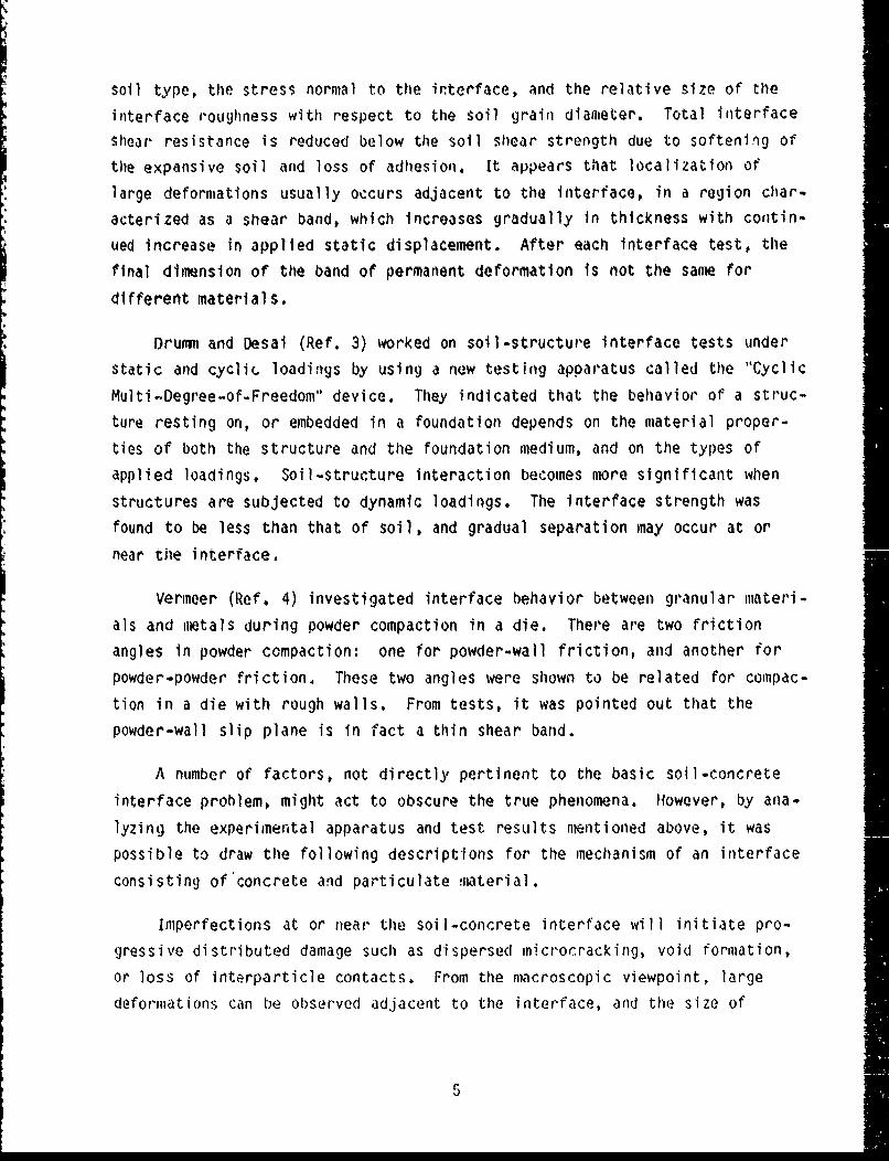
ui = ui + s v +4S a, (46)2

n+1 . n n )n+vi -i + I -)ai + i J(7

To introduce numerical damping, a value of a = 0.8 was used. In addi-

tion, Eq. 42 is approximated with the equation

Mij a!+1 = fn+1 8a (48)

Hence, for given initial and boundary conditions, the field variable u.

at each node can be found without determining the tangent stiffness matrix.

With the use of the constitutive subroutine mentioned earlier, the algorithm

for obtaining the dynamic response of the soil is as follows:

Step 1--Input material constants and control parameters.

Step 2--Input initial and boundary conditions.

Step 3--Start time integration with time step (s):

t n . tn" 1 + s

Step 4--Calculate displacements at each node (i):

u n =un-1 +svn-, S2 an-1i n: Ul + S v s2 an i = 1, 2,..., nn

i i i 2 i

and replace u, at the end of the soil bar by the given boundary

condition.

30

Step_5--Find total strains and strain increments at each element (i) by

using

n nU ~ ""ui

Yn i +1 nn*i' " i = 1, 2,..., nnl - 1"-

and

A'y - Yi

Step 6--Compute inelastic strain gradients at each element (i) according

to the following relation:

-i (1;+1 )f - in'(gi) = _ i = I, 2,..., N-ih

Step 7--Call constitutive subroutine to get the stresses (T).1

Step 8--Calculate the force vector at each node (i) by means of Eq. 44.

Step 9--Calculate accelerations at each node:

an 1 f naI M ii I

where mii is the diagonal element of the diagonal mass matrix.

Step 10--Calculate the velocity vector:

v1 = v1 " + s (1 - c) ai + . a

Step 11--If the results T(x,t) and y(x,t) are needed--print out, then go

to Step 3.

To verify the current approach, comparisons with other existing data were

required. Existing experimental data, however, do not show the relation

31

SVW -N. L. N V I U ' .h.. ýn_--

between the size of the localization zone and the applied load. An alternate

theoretical approach (Ref. 12) with a nonlocal continuum, called an imbricate

continuum, illustrates numerically the dynamic response of a one-dimensional

bar subjected to tensile waves. Two tensile waves are initiated at the ends

of the bar, then the waves meet together at the middle point. That point will

be the first to go into the postpeak regime. Other material points of the bar

near the middle point will also get into the postpeak regime because of the

nonlocal approach. Thus, the strain softening accompanied by localization can

be simulated. In the imbricate continuum model, a bilinear stress-strain

relation is adopted. Although the problem of the soil-concrete interface

seems to be different from that in Reference 12, the basic features are the

same in both cases if the middle point of the one-dimensional bar is changed

to a rigid constraint, and only half the bar length is considered. Therefore,

the numerical solutions of Reference 12 can be used to corroborate the inter-

face model by taking the concrete part as a rigid body and applying the cur-

rent constitutive model to the soil part, as shown in Figure 7.

By dividing the soil bar of length (L a 1) into 20 elements, using the"- 4. 4•,, 4 othr armeer the fol• 1.....

time step s - 0.2 h Vpik, and assigr4iug to 1 other parametrs.Cu o -

ing values:

L = 0.16 0-LS =

a, 0 a. = 0.1 a, = 0.08

a4 =o0.1 / a, = 0.6 n = 0.4

an approximate solution is obtained. Results are shown in Figures 8 to 19.

For purely elastic behavior, Figure 8 shows the propagation of the stress

wave at various times for

EG I I1 p I = 0.4 HCt]

2(1 + L

L0 O.9 / Lp=F -

/-32

32 :

... t ' 1.7- ------ t- i

t 0.5

-J

0.5

r//I

!I

0 0.5

X-coor~dinate, 5.L

Figure 8. Illustration of elastic stress wave at various times.

33

- l - A - I -- - -/ - - - -

/-/ /7.

/' ~/

0.5 /

"-�. . . . t 13.3

/,

- t /

/'/~/

/ /

050 100

X-coordi nate

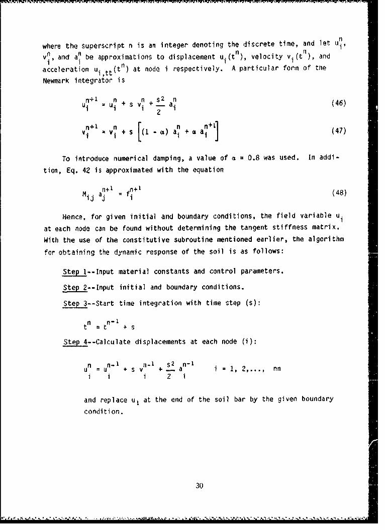
Figure 9. Spatial distribution of stress at various times

(from Ref. 12).

34

t4 .

t 1.2

t 1.

/00 .I-

/ l

I /0.5 0

' !E

I It l'

F 1o tis .7I -_

/ , tppra.h

, 3/ /

I• /

0o I .. IL.•.-•" I |, , 1 . I0 0.5

X-coordi nate, i-X

Figure 10. Spatialth uretdistribution apocof stress at various times using

thecurenIapIoahI

100

1 t a 13.3

t = 25.6

t -74.9

t - 100.0

4-J

JI

t im (. R

3 - - -

50 I 00

X-coordl nate

Figure ].1. Spatial distributions of displacement field at varioustimes (from Ref. 12).

36

II I I

*...... t = 0.4

t-0.8t = 1.2

t = 1.5

t = 1.7

0.5 7

--. e "Po 101,

0 o

0 0.5

X-coordinate, _x

L

Figure 12. Spatial distribution of displacement field at varioustimes using the current approach.

37

4

St= 13.3

t - 25.6

t - 50.3

t = 74.9

t - 100.0

I._

4 A

"S I Ii

-1 -t.. /".j/ii 10

40

so 100

X-coordi nate

Figure 13. Spatial distribution of strain at various times(from Ref. 12).

38

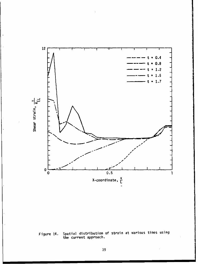
12

.... t x 0.4

-. . . t = 0 .8

-. . t a 1.2t 1.5

t =1.7.

0

N " •. - .

/ ~/_

0o 1 . I I .4 . I L I I I0 0.5

X-coordinate, x

Figure 14. Spatial distribution of strain at various times usingthe current approach.

39

g0

1.5-

10 -

CA

eL

4.4Uv

0.5-

0 4 8

Shear strain, -.

e eEL

Figure 15. Shear stress-strain path for element 1 at time t 1.7.

40

1.5 I II i I I I i I i

1.0

0 4

Shear strain, EL

Figure 16. Shear stress-strain path for element 20 at time t 1.7.

41

I -I- i - - . .

0.5Y

CL

-e 5

----- e 10t

e 20

00 -

xX-coordinate,-L

Figure 17. Distribution of displacement at t = 1.7 for different meshes.

42

I -.. - I ' I . .

......... . .

L- 0.5

- -e = 10

e =20

00.5

X-coordinate, xL

Figure 18. Distribution of stress at t = 1.7 for different meshes.

43

12 1 1

-.... e = 5

- - e = 10

e - 20

4.)

e=0

0 -vi

01 I J j 1I I

0 0.5

X-coordinate, -

L

Figure 19. Distribution of strain at t = 1.7 for different meshes.

44

The material parameters (G and p) are chosen so that the wave speed equals

unity. Except for numerical dispersion and dissipation, the approximate solu-

tion is a reasonable representation of the exact shear wave.

Figures 9 to 14 show the inelastic solutions and the one-to-one compari-

sons with numerical solutions of Reference 12 for

G = E =2 p 2 fL a 0.9 Hit)2(1 + v)

Lo = 0.5 T Lp -

From these figures, it is apparent that the tendencies of the dynamic

responses of the two problems are alike, but with the simpler computational

approach given by the current model. When the shear wave, which propagates

from the right end of the soil bar, reaches the interface, a reflection occurs

and the stress increases to the limit state which initiates softening. As the

figures show, the region next to the interface is characterized by large

strait, and low stress, which is believed to be representative of what occurs

at an interface.

Figures 15 and 16 show the stress-strain responses at t z 1.7 of ele-

ment 1 and element 20, which represent points near the interface and near the

free end of the soil bar. Figures 17 to 19 show the convergence of the numer-

ical solution by using different finite element meshes.

Although there is some numerical noise in the numerical solution, the

localization zone, i.e., the large deformation band with stress being reduced,

can be predicted near the soil-concrete interface. In addition, it appears

that good results can also be obtained by using a coarse mesh.

STATIC RESPONSE OF THE INTERFACE UNDER SHEAR

The global response of the soil-concrete interface under static shear

loading is investigated in this final subsection. The problem geometry isshown in Figure 1. The soil bar is divided into 10 linear elements, and the

45

load is a monotonically increasing displacement at x .L. The shear strength

of the interface is assumed to be slightly smaller than other parts of tlhe

soil bar so that the interface will initiate failure.

The algorithm used for getting the static response of the interface is

outlined as follows:

Ste 1--Input material constants, boundary conditions, and control

parameters.

Step 2--Monotonically increase the strain in the first element, and find

the corresponding increment of stress, which must be the same for every

element.

Step 3--Call the constitutive equation subroutine for each element. If

the results are required, print them out.

Step 4--If the interface is still in the prepeak regime, go to Step 2.

Otherwise, go to Step 5.

Step 5--If the previous value of stress for any element is larger than

the current peak stress corresponding to that element, go into the softening

regime. Otherwise, use elastic unloading.

Step 6--Go to Step 2 for the next increment of strain in the first

element.

Figures 20 to 27 show the numerical solutions for the following

parameters :

L. = 0.5 FT Lp =/3 n = 0.5

G = - 2 :0. 16 L=2(1 + v) L L S

= 10-4 a2 = 0.1 a 3 = 0.1

a,, = 0.1 Ay = 0.05 a, = 0

a, = 0.6

46

L4-)

0 I I I I i

0 0.5X

X-coordinate, -L

Figure 20. Strain distribution for st.:,tic response in elastic regime.

47

40

2 -

•- 20 -

0 - .I .1_. _ I I

0 0.5 1

X-coordi nate, -X

L

Figure 21. Strain distribution for static response in softening regime.

48

0 0.5

LL

.1.

X-.coordinate, .x_

L

Figure 22. Stress distribution for static response in softening regime.

49

1.0

€,.

0.5

0 8 16

Shear strain, -EL

Figure 23. Shear stress-strain response of element 1.

50

1.5 5

1.0

__

L

4-

0i

0.5-

"0 8 16Shear strain ---

'eEL

Figure 24. Shear stress-strain response of element 6.

51

1.0

46

' 0.5

0• ,, * t ! p ! I I S . 1 I I I I I

0 8 16Shear strain, e

eEL

Figure 25. Shear stress-strain response of element 10.

52

40-,

e --10

--- e = 20e= 40

200

4j

L.L

0 0.53

X-coordinate, ~L

Figure 26. Strain distribution for different meshes to show convergence.

53

40 , ,,, -

as =-0.2

as = 0.1

a3= 0

20

00 0.5

X-coordinate, x

L

Figure 27. Effect of the parameter a3 , or the invariant of strain gradient,

on the static response near the interface.

54

Figure 20 shows the strain distribution of static response in the elastic

regime where the strain distribution is uniform. Figure 21 shows the strain

distribution of the static response in the postpeak regime. Note that the

strain distribution is not uniform, and that the localization zone occurs near

the interface. Figure 22 shows the stress distribution that corresponds to

the strain distribution of Figure 21. Since there is no distributed applied

force, the stress distribution is always uniform under static loading. Fig-

ures 23 to 25 show the stress-strain responses of element 1, element 6, and

element 10, respectively. Element 1 represents the region near the interface,

and element 10, the opposite end of the soil bar. After the peak state, ele-

ment 6 unloads elastically at first, and then goes into the softening regime.

Figure 26 shows the convergence of strain distributions for different finite

element meshes. Figure 27 shows the effect of strain gradients on the static

response of the soil bar as reflected through various values of a 3 . For a3 =

0, i.e., local continuum approach, the localization zone cannot be predicted.

This is why a classical local constitutive model cannot simulate the soil-

concrete interface.

Figure 28 shows the relations between shear force and displacement under

the effect of different mean pressures, a1 P, for

-ieL -0.4 a = 0.5 a, = 0.02

with other parameters being unchanged. According to experimental results

reported by Drumm and Desai (Ref. 3), basic features of the static response

near the interface are simulated with this approach.

55

1.50

/ =/ N•-'-•

1.0

0==5

LL

565

----- a1P = 0.2a1 P = 0

05Displacement, --

L

F~iqure 28. Shear stress versus the displacement of the end of the soil

bar for various values of mean pressure. -

56

V. CONCLUSIONS

It was assumed that no relative slip occurs at the contact, surfacebetween soil and concrete. Instead, a shear band appears adjacent to theinterface. The shear band is just the physical representation of soften~ngand localization. The interface serves as an initiator of strain softening.

Through numerical testing and indirect comparisons, it was concluded that

the new nonlocaI constitutive model can simulate the softening behavior of

different materials by selecting appropriate values of material parameters.The approach displays the same features as those in Reference 12, but with amuch simpler computational procedure. Numerical solutions under dynamic and

static shear loadings illustrate the perceived characteristics of a soil-

concrete interface.

Because of the difficulties in measuring the localization zone with high

strain gradients, existing experimental data are not satisfactory. Once goodexperimental data are available, it will be necessary to verify the model, not

• - •~~4 M a-s - a ' t w o -s ansh •I. .,o n l y i n o n e - d i m e n s i o n a l , b u . ...- i n t o n h e -d ,,,, n ,, o , , .. . c a s e s . . . .4 acurved interfaces. Further progress on understanding interface phenomena willrequire a combination of experimental and theoretical investigations. Theresearch reported here indicates that a nonlocal constitutive model is a

promising theoretical approach.

57

REFERENCES

1. Huck, P. J., Liber, T., Chiapetta, R. L., Thomopoulos, N. T., and Singh,N. M., Dynamic Response of Soil/Concrete Interfaces at High Pressure,Technical Report No. AFWL-TR-73-264, Air Force Weapons Laboratory,Kirtland Air Force Base, NM, 1973.

2. Huck, P. J., and Saxena, S. K., "Response of Soil-Concrete Interface atHigh Pressure," Proc. Xth Int. Conf. Soil Mech. Found. Engng.,Stockholm, Sweden, June, 1981.

3. Drumm, E. C., and Desai, C. S., "Testing and Constitutive Modeling forInterface Behavior in Dynamic Soil-Structure Interaction," Report toNational Science Foundation, Washington, D. C., 1983.

4. Vermeer, P. A., "Frictional Slip and Non-associated Plasticity,"Scandinavian Journal of Metallurgy, Vol. 12, 1983, pp. 268-276.

5. Hadjian, A. H., Luco, J. E., and Tsai, N. C., "Soil-Structure Inter-action: Continuum or Finite Elements?", Nuclear Engineering andDesign, Vol. 31, 1974, pp. 151-167.

6. Seed, H. B., Lysmer, J., and Hwang, R., "Soil-Structure Interaction Anal-yses for Seismic Response," Journal of the Geotechnical EngineeringDivision, Proceedings of ASCE, Vol. 101, No. G75, May, 1975.

7. Desai, C. S., and Siriwardane, H. J., Constitutive Laws for EngineeringMaterials with Emphasis on Geologic Materials, Prentice-Hall, Inc.,1984.

8. Oden, J. T., and Pires, E. B., "Numerical Analysis of Certain ContactProblems in Elasticity with Non-classical Friction Laws," Computers andStructures, Vol. 16, No. 1-4, 1983, pp. 481-485.

9. Valanis, I. C., "On the Uniqueness of Solution of the Initial Value Prob-lem in Strain Softening Materials," Journal of Applied Mechanics,Vol. 52, No. 3, September, 1985, pp. 649-653.

10. Sandler, I., and Wright, J., "Summary of Strain-Softening,' TheoreticalFoundations for Large-Scale Computions of Nonlinear Material Behavior,Preprints, DARPA-NSF Workshop, S. Nemat-Nasser, ed,, Northwestern Univer-sity, Evanston, ll!inois, October, 1983, pp. 225-241.

11. Read, H. E., and Hegemier, G. A., "Strain Softening of Rock, Soil andConcrete," Mechanics of Materials Vol. 3, 1984, pp. 271-294.

12. Bazant, Z. P., Belytschko, T. B., and Chang, T., "Continuum Theory forStrain Softening." Journal of Engineering Mechanics, Vol. 110,No. 12, December, 1984.

13. Schreyer, H. L., and Chen, Z., "One-Dimensional Softening with Localiza-tion," Journal of Applied Mechanics, (accepted for publication).

14. Schreyer, H. L., The Application of Plasticity and Viscoplasticity toMetals and Frictional Materials, Course Notes, ME 544, University ofNew Mexico, 1985.

58

15. Becker, E. B., Carey, G. F., and Oden, J. T., Finite Elements--AnIntroduction, Prentice-Hall, Inc., 1981.

16. Ohatt, G., and Touzot, G., The Finite Element Method Displayed, JohnWiley & Sons, Inc., i984.

59

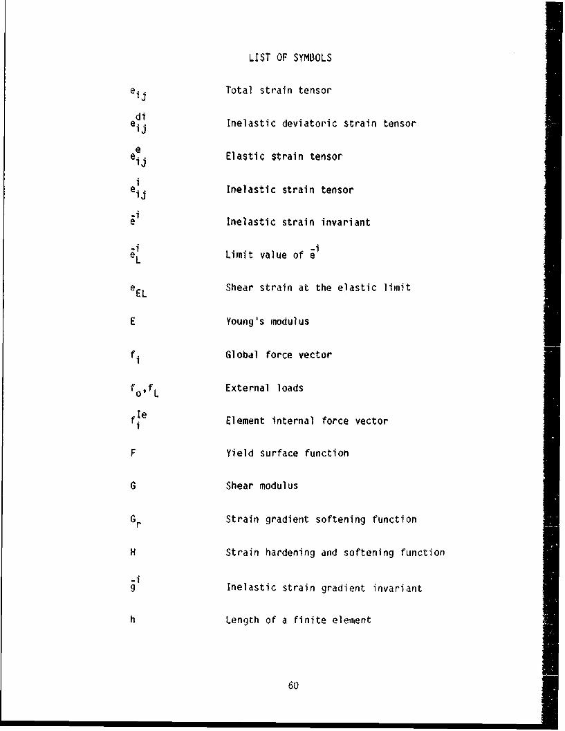
LIST OF SYMBOLS

eij Total strain tensor

diedi Inelastic deviatoric strain tensor

e ej Elastic strain tensor

ii Inelastic strain tensor

-ii Inelastic strain invariant

-ieL Limit value of e

eEL Shear strain at the elastic limit

E Young's modulus

f i Global force vectorX/Io'fL External loads

fle Element internal force vector1

i"

F Yield surface function

G Shear modulus

Gr Strain gradient softening function

H Strain hardening and softening function

-ig Inelastic strain gradient invariant

h Length of a finite elemrnent

60

L Length of a soil bar

Lo 0Elastic limit of yield surface

Lp Peak value of yield surface

Me, Element mass matrixij

Mij Global mass matrix

n Material parameter

P Mean pressure

s Time step in time integration

ui Global displacement vector

vi Global velocity vector

w Weighting function

Y Engineering shear strain

Aeij Total strain increment tensor

eaeie Elastic strain increment tensorij

Ae• iInelastic strain increment tensor

V Poisson's ratio

Mass density

Oij Stress tensor

T Engineering shear stress

61/62